Upper bounds on the highest phonon frequency and superconducting temperature from fundamental physical constants

Abstract

Fundamental physical constants govern key effects in high-energy particle physics and astrophysics, including the stability of particles, nuclear reactions, formation and evolution of stars, synthesis of heavy nuclei and emergence of stable molecular structures. Here, we show that fundamental constants also set an upper bound for the frequency of phonons in condensed matter phases, or how rapidly an atom can vibrate. This bound is in agreement with ab initio simulations of atomic hydrogen and high-temperature hydride superconductors, and implies an upper limit to the superconducting transition temperature $T_{c}$ in condensed matter. Fundamental constants set this limit to the order of 10${}^{2}-10^{3}$ K. This range is consistent with our calculations of $T_{c}$ from optimal Eliashberg functions. As a corollary, we observe that the very existence of high-temperature superconductivity research is due to the observed values of fundamental constants. We finally discuss how fundamental constants affect the observability of other condensed matter phenomena including phase transitions.

1 Introduction

The governing role of fundamental physical constants has been extensively discussed in high-energy particle physics and astrophysics. Examples include the stability of nuclei, nuclear reactions, and the formation and evolution of stars – where heavy elements are produced and give rise to other observable structures. In these and other processes, fundamental constants give the Universe its observed properties and separate it from potential others Barrow (2003); Barrow and Tipler (2009); Carr and Rees (1979); Carr (2009); Sloan et al. (2022); Cahn (1996); Hogan (2000); Adams (2019); Uzan (2003). Understanding the origin of fundamental constants and their fine-tuning is considered one of the grand challenges in science Barrow and Webb (2006); Weinberg (1983). Approaching this challenge starts with deepening our understanding of how fundamental constants affect phenomena spanning the length and energy scales between particle physics and astrophysics Trachenko (2023a); Brazhkin (2023); Trachenko (2023b).

In condensed matter physics and in other areas that support a continuum description of matter, such as elasticity and hydrodynamics, system properties are driven by many-body collective effects. These effects are often considered as emergent and thus not reducible to individual particles whose properties are set by fundamental constants. It was therefore unexpected when it was discovered that fundamental constants govern the bounds, characteristic values and properties of several key many-body collective processes. Examples include viscosity Trachenko and Brazhkin (2020), diffusion and spin dynamics Luciuk et al. (2017); Sommer et al. (2011); Bardon et al. (2014); Trotzky et al. (2015); Enss and Thywissen (2018), electron and heat transport Hartnoll (2015); Mousatov and Hartnoll (2020); Behnia and Kapitulnik (2019), thermal conductivity in insulators Trachenko et al. (2021) and conductors Brazhkin (2023), the speed of sound Trachenko et al. (2020), elastic moduli including those in lower-dimensional systems Brazhkin (2023); Trachenko (2023a), thermal expansion, melting Trachenko (2024) and velocity gradients that can be set up in cells using biochemical energy Trachenko (2023c). In these examples, properties are governed by either fundamental constants only or by a combination of these constants with other parameters such as temperature. The implications of these findings extend to both fundamental and applied science Trachenko (2023a).

Here, we show that fundamental physical constants provide an upper bound to the frequency of phonons in condensed matter phases, setting a limit to the vibrational frequency of atoms. This bound involves the dimensionless electron-to-proton mass ratio $\beta$, the key constant involved in setting the finely-tuned “habitable zone” of our world in the ($\alpha$, $\beta$) space, where $\alpha$ is the fine-structure constant Barrow (2003). We find this bound to be in agreement with ab initio simulations of atomic hydrogen and hydride superconductors which, as hydrogen is the lightest nucleus (a single proton), host the highest possible phonon frequencies. We subsequently show that this upper bound in the maximal phonon frequency implies an upper bound to the phonon-mediated superconducting critical temperature $T_{\mathrm{c}}$ in condensed matter. In particular, we show that fundamental constants set the upper bound to $T_{c}$ on the order of $10^{2}-10^{3}$ K, consistent with calculations of $T_{c}$ from optimal Eliashberg functions. We also observe that in addition to electron-phonon coupling, the bound to $T_{c}$ in terms of fundamental constants applies to other coupling mechanisms such as electron-electron coupling. This implies that the current search for $T_{\mathrm{c}}$ at and above $300$ K is itself due to fundamental constants taking their observed values. We finally observe that fundamental constants affect the observability of other phenomena in condensed matter physics including phase transitions.

2 Upper bound on the vibrational frequency

We start with the upper bound on the vibrational frequency. Oscillations are ubiquitous in nature and play a central role in all areas of physics, including condensed matter physics. The question of how high the oscillation frequency of an atom can be in solids or liquids is therefore of general importance.

The maximal frequency in a given system, $\omega_{\mathrm{m}}$, is the largest frequency in the phonon dispersion, and is typically close to the Debye frequency $\omega_{\rm D}$. We are interested in an upper bound, $\omega_{\mathrm{m}}^{\mathrm{u}}$, on this maximal frequency (and thus an upper bound on all phonon frequencies). We recall two important properties of condensed matter phases: the interatomic separation $a$ and a cohesive, or bonding, energy $E$. The Bohr radius, $a_{\rm B}$, sets the characteristic scale of $a$ to the order of Angstroms:

$$a_{\rm B}=\frac{4\pi\epsilon_{0}\hbar^{2}}{m_{e}e^{2}}$$ (1)

and the Rydberg energy, $E_{\rm R}=\frac{e^{2}}{8\pi\epsilon_{0}a_{\rm B}}$ Ashcroft and Mermin (1976), sets the characteristic scale of $E$ to the order of several eV:

$$E_{\rm R}=\frac{m_{e}e^{4}}{32\pi^{2}\epsilon_{0}^{2}\hbar^{2}}$$ (2)

where $e$ and $m_{e}$ are electron charge and mass.

The ratio $\frac{\hbar\omega_{\mathrm{m}}}{E}$ can be derived by approximating $\hbar\omega_{\mathrm{m}}$ as $\hbar\left(\frac{E}{ma^{2}}\right)^{\frac{1}{2}}$, where $m$ is the atom mass and then either (a) using $a=a_{\rm B}$ from (1) and $E=E_{\rm R}$ from (2) or (b) using $E=\frac{\hbar^{2}}{2m_{e}a^{2}}$. This gives, up to a factor of order one, the following relation:

$$\frac{\hbar\omega_{\rm m}}{E}=\left(\frac{m_{e}}{m}\right)^{\frac{1}{2}}$$ (3)

The same ratio (3) follows by combining two known relations in metallic systems: $\frac{\hbar\omega_{\rm m}}{E}\approx\frac{c}{v_{\rm F}}$, where $v_{\rm F}$ is the Fermi velocity and $c$ is the speed of sound, and $\frac{c}{v_{\rm F}}\approx\left(\frac{m_{e}}{m}\right)^{\frac{1}{2}}$, providing an order-of-magnitude estimation of $\frac{\hbar\omega_{\rm m}}{E}$ in other systems too Ashcroft and Mermin (1976).

The upper bound $\omega_{\rm m}^{\rm u}$ is obtained from Eq. (3) by setting $m=m_{p}$, the proton mass, corresponding to atomic hydrogen. Combining this with Eq. (2) yields finally

$$\omega_{\rm m}^{\rm u}=\frac{1}{32\pi^{2}\epsilon_{0}^{2}}\frac{m_{e}e^{4}}{\hbar^{3}}\left(\frac{m_{e}}{m_{p}}\right)^{\frac{1}{2}}$$ (4)

Interestingly, $\omega_{\rm m}^{\rm u}$ in (4) can also be written in terms of the Compton frequency $\omega_{\rm C}=\frac{m_{e}c^{2}}{\hbar}$ and the fine structure constant $\alpha=\frac{1}{4\pi\epsilon_{0}}\frac{e^{2}}{\hbar c}$ as

$$\omega_{\rm m}^{\rm u}=\frac{1}{2}\omega_{\rm C}\alpha^{2}\left(\frac{m_{e}}{m_{p}}\right)^{\frac{1}{2}}$$ (5)

Equation  (5) offers a simple result showing that the upper bound to the atomic oscillation frequency is set by the Compton frequency times the square of $\alpha$ and the square-root of the electron-to-phonon mass ratio.

Equation  (4) sets $\omega_{\rm m}^{\rm u}$ in terms of fundamental physical constants. The constants $\hbar$, $m_{e}$, and $e$ determine the electromagnetic energy scale driving atomic oscillations. The proton mass $m_{p}$ is intrinsic to the atoms being driven and sets the scale (both in time, and space) of the oscillatory response. Interestingly, $\omega_{\rm m}^{\rm u}$ involves the electron-to-proton mass ratio $\beta=\frac{m_{e}}{m_{p}}$. This dimensionless constant is considered of fundamental importance: together with the fine-structure constant, it sets a finely-tuned habitable zone in ($\alpha$, $\beta$) space where it governs the stability of molecular structures, processes involved in igniting and fuelling stars (and thus the production of heavy elements), and other essential effects giving rise to our observable world Barrow (2003).

With $E_{\rm R}$=13.6 eV and $\beta=\frac{m_{e}}{m_{p}}=\frac{1}{1836}$, $\omega_{\rm m}^{\rm u}$ in Eq. (4) is about (here and below, $k_{\rm B}=1$):

$$\omega_{\rm m}^{\rm u}=3680\,\rm{K}$$ (6)

Equations  (4)-(6) show that fundamental constants set $\omega_{\rm m}^{\rm u}$ on the order of $10^{3}$–$10^{4}$ K, a result we will use to discuss phonon-mediated superconductivity below. The upper bound $\omega_{\rm m}^{\rm u}$ in (6) is of the same order of magnitude, but above, the experimental Debye frequency $\omega_{\rm D}$ of 2240 K in ambient pressure diamond Tohei et al. (2006), the hardest known material Brazhkin and Solozhenko (2019).

The upper bound (4)-(6) corresponds to solid hydrogen with strong metallic bonding. Although this phase only exists at megabar pressures Dias and Silvera (2017); Loubeyre et al. (2020); McMahon et al. (2012) and is thermodynamically and dynamically unstable at ambient pressure, it is interesting to check the validity of our bound and calculate $\omega_{\rm m}$ in atomic hydrogen. The importance of this calculation is also highlighted by the strong interest in the properties of atomic hydrogen at high pressure (see, e.g., Refs. Dias and Silvera (2017); Loubeyre et al. (2020); McMahon et al. (2012)).

Before calculating $\omega_{\rm m}$, we first evaluate the effect of pressure on the fundamental bound (4) because solid atomic hydrogen exists at high pressure only as mentioned above. We make two remarks in relation to the pressure effect. First, hydrogen is a unique element with no core electrons. As compared to heavier elements, this gives weaker repulsive contributions to the interatomic interaction and weaker pressure dependence of elastic moduli Brazhkin and Lyapin (2002). As a result, pressure has a weaker effect on $\omega_{\rm m}$ in hydrogen as compared to other systems. Second, the effect of pressure on $\omega_{\rm m}^{\rm u}$ can be approximately estimated by adding the term $PV$ to $E$ in Eq. (3), representing the work needed to overcome the elastic deformation Frenkel (1947) due to external pressure in order to surmount the energy of cohesion. Here, $V$ is the elementary volume on the order of $a^{3}$. According to Eqs. (3)-(4), this increases $\omega_{m}^{u}(P)$ as

$$\omega_{\rm m}^{\rm u}(P)=\omega_{\rm m}^{\rm u}+a^{3}\left(\frac{m_{e}}{m_{p}}\right)^{\frac{1}{2}}P$$ (7)

We calculate the phonon dispersion curves of atomic hydrogen in the $I4_{1}/amd$ structure Nagao et al. (1997); Pickard and Needs (2007), which is currently the best candidate structure for solid atomic metallic hydrogen. This structure is calculated to become thermodynamically stable in the pressure range $400$–$600$ GPa Azadi et al. (2014); McMinis et al. (2015); Monacelli et al. (2023), below which solid hydrogen is a molecular solid. We perform density functional theory (DFT) calculations using the castep package Clark et al. (2005). Details of DFT calculations are given in the Appendix.

A representative phonon dispersion for atomic hydrogen at $400$ GPa is shown Fig. 1, with the maximal phonon frequency occuring at the N point of the Brillouin zone with reciprocal space coordinates $(0,\frac{1}{2},0)$. The maximal frequencies in the calculated phonon dispersion curves are shown in Fig. 2 as a function of pressure, and they are located at the N point for pressures below about 600 GPa and at the $\Gamma$ point for pressures above that value. The lowest pressure depicted corresponds to a pressure above the dynamical stability range of the atomic hydrogen structure. The diagram in Fig. 2 also shows the upper bound (6) and $\omega_{\rm D}$ in diamond.

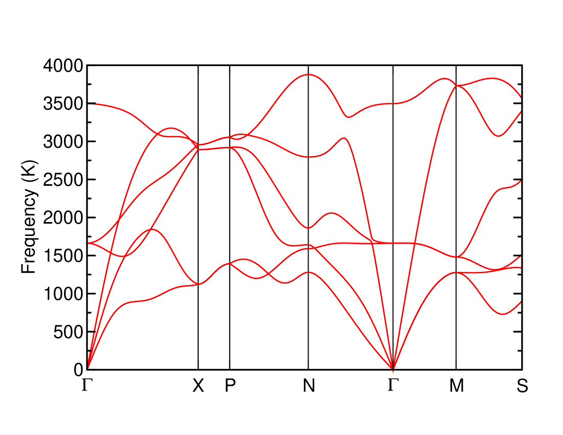
Figure 1: Phonon dispersion of atomic hydrogen calculated at $400$  GPa.

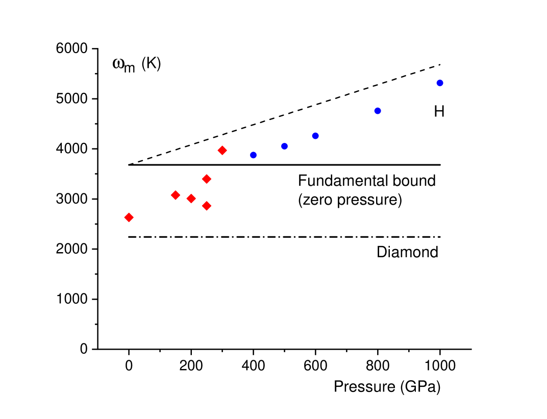
Figure 2: Maximal phonon frequency as a function of pressure for different systems. Blue bullet points show the calculated maximal phonon frequencies in atomic hydrogen at the corresponding pressures. Red diamonds show the maximal phonon frequencies in a range of hydrides at different pressures, which are, from left to right: MgIrH₆ Doliu et al. (2024), MgVH₆ Zheng et al. (2021), CaH₆ Jeon et al. (2022), LaH₁₀ (top) Durajski et al. (2020), H₃S (bottom) Sano et al. (2016), and SrH₁₀ Tanaka et al. (2017). The horizontal solid black line shows the fundamental bound $\omega_{\rm m}^{\rm u}$ (6). The horizontal dash-dotted line shows the Debye frequency of diamond at ambient pressure. The dashed line on top of the graph shows $\omega_{\rm m}^{\rm u}(P)$ in Eq. (7) with $a=2a_{\rm B}$.

We observe in Fig. 2 that the calculated $\omega_{\rm m}$ is only slightly above $\omega_{\rm m}^{\rm u}$ at the high pressure of 400 GPa in atomic hydrogen. Assuming a pressure-independent effective $a$ in Eq. (7) for estimation purposes, we find that $\omega_{\rm m}^{\rm u}(P)$ lies close and above the hydrogen points if $a$ is taken to be about $2a_{\rm B}$ (see dashed black line in Fig. 2). This is consistent with the elementary volume being related to the Bohr radius and fundamental constants. Although $a=2a_{\rm B}$ in Eq. (7) introduces an ad hoc choice, the dashed line in Fig. 2 demonstrates that the pressure effect on $\omega_{\rm m}^{\rm u}$ can be accounted for with a sensible and physically justified choice of $a$. In this regard, we note more generally that evaluating bounds on many important condensed matter properties using fundamental constants only inevitably involves approximations Trachenko (2023a); Brazhkin (2023). This includes $\omega_{\rm m}^{\rm u}$ in Eqs. (4)-(6) which use approximate relations such as Eq. (3). Nevertheless, we see that the upper bound $\omega_{\rm m}^{\rm u}$ is in good agreement with computational results.

In addition to atomic hydrogen with the lightest atomic mass, another appropriate test for the theoretical upper bound $\omega_{\rm m}^{\rm u}$ in Eq. (4) involves the comparison with hydrogen-rich systems. These include hydride superconductors at high pressure, which have been of interest recently because they exhibit the highest superconducting critical temperature $T_{c}$ currently known Flores-Livas et al. (2020); Duan et al. (2017); Pickard et al. (2019). For our assessment of the maximal frequency upper bound, we chose a range of hydrides based on their chemical and structural variety as well as a wide range of pressures at which phonons have been previously calculated using ab initio methods. Our list includes data on LaH₁₀ Durajski et al. (2020) and H₃S Sano et al. (2016), with the highest experimentally measured $T_{c}$, two other binary hydrides CaH₆ Jeon et al. (2022) and SrH₁₀ Tanaka et al. (2017), and two ternaries MgIrH₆ Doliu et al. (2024) and MgVH₆ Zheng et al. (2021). The maximal phonon frequencies extracted from the calculated dispersion curves of these hydrides are shown in Fig. 2 as red diamonds. We observe that most points are below the fundamental bound $\omega_{\rm m}^{\rm u}$. The maximal frequency in SrH₁₀ at the highest pressure of 300 GPa exceeds the fundamental bound (6) but is below the bound accounting for the pressure effect (7).

3 Superconducting temperature and search for room-temperature superconductivity

3.1 Upper limit to $T_{c}$

We now discuss the implications of the upper bound of $\omega_{\rm m}$ for phonon-mediated superconductivity and the superconducting critical temperature $T_{c}$. Upper bounds of $T_{c}$ have been discussed on the basis of different mechanisms and have been related to various system properties, including the electron-phonon coupling constant $\lambda$, the energy distribution of valence electrons, the phonon and Fermi energies, phonons and other instabilities, phase fluctuations, and stiffness (see, e.g., Refs. McMillan (1968); Moussa and Cohen (2006); Liu et al. (2022); Varma (2012); Esterlis et al. (2018a, b); Hazra et al. (2019); Chubukov et al. (2020) and references therein). More recent work has offered model examples where these bounds can be exceeded Hofmann et al. (2022).

Our results on the maximal phonon frequency suggest that the upper limit for $T_{c}$ in phonon-mediated superconductors may be governed at a deeper level by fundamental physical constants. We first consider the Migdal-Eliashberg (ME) theory of superconductivity involving the electron-phonon coupling relevant to high $T_{c}$ in hydrides. We will later discuss the alternative electron-electron coupling mechanism for superconductivity.

In the ME picture, $T_{c}=C\,\overline{\omega}$, where $C$ is a slowly-varying monotonically increasing function of $\lambda$ and $\overline{\omega}$ is an averaged phonon frequency Moussa and Cohen (2006); Carbotte (1990). More recent work explored effects beyond the ME theory and noted that they may be inessential for the superconducting state and $T_{c}$ Chubukov et al. (2020). There are several other interesting insights related to the effects of phonons and $\lambda$ on $T_{c}$. First, depending on the system, different phonon modes may contribute differently to $\lambda$ and $T_{c}$. This has been recently discussed in hydrides where different hydrogen-dominated modes combine with other element-dominated modes to set $\lambda$ Durajski et al. (2020); Sano et al. (2016); Tanaka et al. (2017); Jeon et al. (2022); Zheng et al. (2021); Doliu et al. (2024). Second, a more general insight is that $T_{c}$ has a maximum at a certain $C$ due to the competition between the increase of $T_{c}$ with $\lambda$ and the suppression of $T_{c}$ due to instabilities at large $\lambda$ Moussa and Cohen (2006); Esterlis et al. (2018b, a); Carbotte (1990). Supported by model simulations, theory, and empirical data, $C$ is found to be $C\approx 0.1$ Esterlis et al. (2018b, a). A similar $C$ in the range $0.1-0.2$ corresponds to $\lambda=1-2$ Moussa and Cohen (2006); Carbotte (1990), which are typical values of $\lambda$ in hydrides under pressure Shipley et al. (2021) where the highest $T_{c}$ is observed Flores-Livas et al. (2020); Duan et al. (2017); Pickard et al. (2019). We are interested in an upper bound for $T_{c}$, hence we substitute the average $\bar{\omega}$ by the maximal phonon frequency $\omega_{\rm m}$. Then, using Eq. (4) for $\omega_{\rm m}^{\rm u}$, the upper bound of $T_{c}$, which we call $T_{c}^{u}$, is

$$T_{c}^{u}=C\omega_{\rm m}^{\rm u}=C\left(\frac{m_{e}}{m_{p}}\right)^{\frac{1}{2}}\frac{1}{32\pi^{2}\epsilon_{0}^{2}}\frac{m_{e}e^{4}}{\hbar^{3}}$$ (8)

Using $\omega_{\rm m}^{\rm u}$ set by fundamental constants in Eq. (6) and $C$ in the above range $0.1-0.2$, Eq. (8) gives $T_{c}^{u}$ in the range $370$–$740$ K and on the order of

$$T_{c}^{u}=10^{2}-10^{3}\,\rm{K}$$ (9)

The scale of $T_{c}^{u}$ in Eqs. (8)-(9) is set by fundamental physical constants (the order of magnitude of $C$ is not variable). This has interesting implications to which we will return later.

The range (9) can be verified numerically by calculating an upper bound within the ME theory directly,

$$T_{c}^{u}\sim\max_{\alpha^{2}F\in S}T_{c}[\alpha^{2}F]$$ (10)

where the functional $T_{c}[\alpha^{2}F]$ is the critical temperature from the solution of the Eliasbherg equations Marsiglio (2020) and $S$ is a set of sensible Eliashberg functions extending to a maximum phonon frequency of $\omega_{\rm m}^{\rm u}$. This optimization is shown in Fig. 3 for a fixed value of $\lambda=2$, and converges to $T_{c}^{u}\sim 600$ K, well within the range of Eq. (9). We see that the optimization proceeds by shifting spectral weight to as high a frequency as possible, confirming that the value of $\omega_{m}^{u}$ is the limiting factor. Details of this optimization procedure are available in the Appendix.

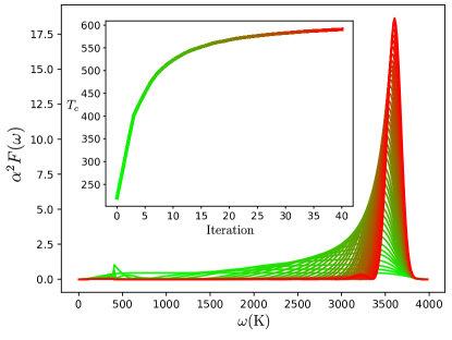
Figure 3: The evolution of the Eliashberg function $\alpha^{2}F(\omega)$ and corresponding $T_{c}$ (inset) as Eq. (10) is optimized. Red (green) lines are later (earlier) iterations in the optimization.

$T_{c}^{u}$ in Eq. (8) can be made more stringent in a particular family of materials such as hydrides. Recall that (a) $E_{\rm R}$ used to evaluate the bonding energy $E$ is larger than bonding energies in real materials and (b) the average mass in real materials is larger than the proton mass $m_{p}$ featuring in Eqs. (4) and (8). Both effects reduce $T_{c}^{u}$. According to Eqs. (3), (4), and (8), the difference between $E$ and $E_{\rm R}$ results in $T_{c}^{u}$ decreasing by a factor $\frac{E_{\rm{eff}}}{E_{\rm R}}$, where $E_{\rm{eff}}$ is the effective bonding energy in the relevant subsystem within a hydride. The difference between the average mass and $m_{p}$ reduces $T_{c}^{u}$ by a factor $\left(\frac{m_{\rm{eff}}}{m_{p}}\right)^{\frac{1}{2}}$, where $m_{\rm{eff}}$ is the effective mass in the relevant subsystem. In hydrogen-rich systems, $m_{\rm{eff}}$ is close to $m_{p}$ and this factor is close to one.

3.2 Other coupling mechanisms

The above discussion also applies to systems where superconductivity is related to mechanisms other than the electron-phonon coupling. For electron-electron pairing, $T_{c}$ depends on the Fermi energy $E_{\rm F}$ and is on the order of about $\frac{E_{\rm F}}{10^{2}}$ Varma (2012); Uemura et al. (1991). $E_{\rm F}\propto\frac{\hbar^{2}}{m_{e}a_{\rm B}^{2}}\propto\frac{m_{e}e^{4}}{\hbar^{2}}$ and depends on fundamental constants as $E_{\rm R}$ in Eq. (2) does. Hence, $T_{c}$ in the electron-electron systems is also governed by fundamental constants as it is in the electron-phonon superconductors.

Assuming that the upper limit to $E_{\rm F}$ is set by $E_{\rm R}$ in Eq. (2) and recalling that $T_{c}$ in the electron-electron systems is on the order of $\frac{E_{\rm F}}{10^{2}}$ Varma (2012); Uemura et al. (1991), we note that the upper bound to $T_{c}$ in these systems is close to $T_{c}^{u}$ since $C\left(\frac{m_{e}}{m_{p}}\right)^{\frac{1}{2}}$ in Eq. (8) with $C\approx 0.1$ is on the order of about $\frac{1}{10^{2}}$.

3.3 Fundamental constants and search for room-temperature superconductivity

Having seen that the overall scale of $T_{c}^{u}$ is set by fundamental physical constants, we now ask the important question of what would be the effects of fundamental constants having different values. This question is intensely researched in high-energy physics and astrophysics and is related to fine-tuning of the Universe and associated grand challenges in modern science Barrow (2003); Barrow and Tipler (2009); Carr and Rees (1979); Carr (2009); Sloan et al. (2022); Cahn (1996); Hogan (2000); Adams (2019); Uzan (2003); Barrow and Webb (2006). How would superconductivity change were fundamental constants (e.g., $\hbar$, $m_{e}$, $e$ and $\frac{m_{e}}{m_{p}}$ in Eq. (8)) to take different values? This question is well-posed because it is possible to change $T_{c}^{u}$ in Eq. (8) by varying $\hbar$, $m_{e}$, $e$ and $m_{p}$ while keeping $\beta=\frac{m_{e}}{m_{p}}$ and $\alpha=\frac{e^{2}}{\hbar c}$ unchanged and hence maintain the rest of essential processes (e.g. those involved in stellar formation and evolution, synthesis of heavy elements, stability of ordered structures and so on) intact Barrow (2003). Were different fundamental constants to give $T_{c}^{u}$ on the order of, for example, $10^{-6}$ K or lower, superconductivity would be unobserved. Were different fundamental constants to give $T_{c}^{u}$ on the order $10^{6}$ K, many superconductors would have $T_{c}$ in excess of 300 K. Consistent with Eqs. (8)-(9) giving $T_{c}^{u}$ on the order of $10^{2}-10^{3}$ K due to currently observed fundamental constants, we observe superconductivity in the temperature range $T\lesssim$ 100-200 K. This understandably stimulates the current research into finding systems with $T_{c}$ of 300 K and above. Therefore, the very existence of the current line of enquiry to identify systems with $T_{c}$ above 300 K is itself due to the values of fundamental constants currently observed.

4 Fundamental constants and observability of phenomena in condensed matter physics

The discussion in the previous section implies that fundamental constants can affect observability of an entire condensed matter phenomenon such as superconductivity. This implication is wider than what was discussed in earlier work Trachenko (2023a); Trachenko and Brazhkin (2020); Trachenko (2023b); Luciuk et al. (2017); Sommer et al. (2011); Bardon et al. (2014); Trotzky et al. (2015); Enss and Thywissen (2018); Hartnoll (2015); Mousatov and Hartnoll (2020); Behnia and Kapitulnik (2019); Trachenko et al. (2021); Brazhkin (2023); Trachenko et al. (2020); Trachenko (2024, 2023c) where fundamental constants were shown to set a bound on a property (e.g., viscosity, thermal conductivity, diffusivity, or speed of sound) which is already observed.

The observability of superconductivity as a result of current values of fundamental constants can be extended more generally to the observability of other phenomena and phase transitions. Indeed, different fundamental constants substantially increasing $\omega_{\rm m}^{\rm u}$ in Eq. (4) would result in $T\ll\hbar\omega_{\rm m}$ and hence $T\ll\hbar\omega_{\rm D}$ ($\omega_{\rm D}$ is Debye frequency) at typical planetary temperatures. This would result in the solid properties being always quantum and the classical regime $T>\hbar\omega_{\rm D}$ unobservable. This would also suppress or arrest second-order structural phase transitions because of the smallness of the phonon entropy when $T\ll\hbar\omega_{\rm D}$ Landau and Lifshitz (1970).

Another example is the first-order melting transition where the characteristic slopes of the pressure-temperature melting lines are set by fundamental constants Trachenko (2024). This implies that different values of these constants would result in melting either (a) always taking place at typical planetary conditions and no solids existing or (b) being unobservable (in this case, the ice melting temperature would be above typical planetary temperatures implying no water-based life).

Linking the discussion the previous paragraph and in Section 3.3, we note that current fundamental constants enable diverse phenomena such as water-based life and superconductivity.

This and similar future discussion deepen our understanding of how fundamental constants affect observability of entire new phenomena at condensed matter length and energy scales. This helps to fill the large gap Trachenko (2023b) between the scales involved in nuclear physics and astrophysics where fundamental constants were shown to give rise to different key effects such as the stability of nuclei, star formation, and heavy nuclei synthesis Barrow (2003); Barrow and Tipler (2009); Carr and Rees (1979); Carr (2009); Sloan et al. (2022); Cahn (1996); Hogan (2000); Adams (2019); Uzan (2003). Observability of each effect and phenomenon imposes constraints on fundamental constants Barrow (2003). Discussing different constraints along a continuous path of length and energy scales, including condensed matter scales, is likely to bring about new insights into understanding fundamental constants.

5 Summary

In summary, we have shown that fundamental physical constants set the upper limit to the vibrational frequency of atoms in condensed phases. This bound is in agreement with simulations of atomic hydrogen and high-temperature superconducting hydrides. We have also proposed that fundamental constants set the upper limit to the superconducting critical temperature on the order of 10²–$10^{3}$ K. This implies that the current line of enquiry to discover superconductors above 300 K is itself due to the observed values of fundamental constants.

Appendix

.1 Density functional theory calculations

In our density functional theory calculations, we use the Perdew-Burke-Ernzerhof (PBE) exchange-correlation functional Perdew et al. (1996), an energy cutoff of $1200$ eV and a $\mathbf{k}$-point grid of spacing $2\pi\times 0.025$ Å^-1 to sample the electronic Brillouin zone. We relax cell parameters and internal coordinates to obtain a pressure to within $10^{-4}$ GPa of the target pressure and forces smaller than $10^{-5}$ eV/Å. We calculate the phonon dispersion using the finite displacement method Kunc and Martin (1978) in conjunction with nondiagonal supercells Lloyd-Williams and Monserrat (2015) with a $4\times 4\times 4$ coarse $\mathbf{q}$-point grid to sample the vibrational Brillouin zone, and we use Fourier interpolation to calculate the phonon frequencies along a high symmetry path in the Brillouin zone.

.2 Optimization of the Eliashberg function

In isotropic Migdal-Eliashberg theory, $\lambda$ is a functional of the Eliashberg function $\alpha^{2}F(\omega)$, specifically

$$\lambda[\alpha^{2}F]=2\int\frac{\alpha^{2}F(\omega)}{\omega}d\omega.$$ (11)

The critical temperature is obtained by solution of the Eliashberg equations Marsiglio (2020), whose only inputs are the Eliashberg function and a value for the Coulomb pseudopotential $\mu^{*}$. We can therefore write $T_{c}=T_{c}[\alpha^{2}F](\mu^{*})$, a functional of $\alpha^{2}F$ and a function of $\mu^{*}$.

We can obtain an upper bound for the critical temperature by extremizing $T_{c}[\alpha^{2}F(\omega)](\mu^{*})$ over a set of sensible $\alpha^{2}F$ functions, for a typical value of $\mu^{*}=0.125$. We note that $\alpha^{2}F(\omega)$ can not extend beyond the maximum phonon frequency in the system: $\alpha^{2}F(\omega>\omega_{m})=0$. For a finite $\lambda$ value, $\alpha^{2}F(\omega)$ must also smoothly approach $0$ as $\omega\rightarrow 0$. Finally, $\alpha^{2}F(\omega)$ must be positive. These form our conditions for a sensible Eliashberg function. As noted in the main text, $\lambda$ is naturally limited to ${\lambda\sim 1-2}$ by instabilities. To calculate an upper bound, we therefore fix $\lambda=2$. For the function space $F$ containing $\alpha^{2}F$, we can construct a map $M:F\rightarrow F$ whose image space satisfies these constraints on $\alpha^{2}F$. That is to say, $\forall f\in F$,

$$\lambda[M(f)] =2,$$ (12)

$$M(f)(\omega) \geq 0\;\forall\omega,$$ (13)

$$\lim_{\omega\rightarrow\omega_{m}}M(f)(\omega) =0,$$ (14)

$$\lim_{\omega\rightarrow 0}M(f)(\omega) =0.$$ (15)

In particular, noting that Eq. 11 is linear in $\alpha^{2}F$, we can satisfy Eq. 12 by taking

$$M(f)=\frac{2E(f)}{\lambda[E(f)]}$$ (16)

For some $E:F\rightarrow F$. We choose

$$E(f)(\omega)=f^{2}(\omega)G(\omega)G(\omega_{m}-\omega)$$ (17)

where mapping $f\rightarrow f^{2}$ ensures positivity (Eq. 13) and $G$ is an envelope function, which we take as

$$G(\omega)=\begin{cases}1-\exp{(-\omega^{2}/\sigma^{2})}\text{ if }\omega>0\\ 0\text{ otherwise}\end{cases}$$ (18)

so that the limits in Eqs. 14 and 15 hold, and are approached smoothly. We take the width of the envelope to be $\sigma=300$ K, but this value makes little difference to the resulting $T_{c}$.

Having constructed $M$, we can perform the constrained optimization of $T_{c}$ as

$$T_{c}^{u}=\max_{f\in F}T_{c}[M(f)](\mu^{*}=0.125)$$ (19)

by representing $f$ on a uniform grid of frequency points and employing the BFGS algorithm Fletcher (1987). We begin the optimization with an initial guess of $f=1$.

merlin.mbs apsrev4-1.bst 2010-07-25 4.21a (PWD, AO, DPC) hacked

References

- Barrow (2003) J. D. Barrow, The Constants of Nature (Pantheon Books, 2003).
- Barrow and Tipler (2009) J. D. Barrow and F. J. Tipler, The Anthropic Cosmological Principle (Oxford University Press, 2009).
- Carr and Rees (1979) B. J. Carr and M. J. Rees, Nature 278, 605 (1979).
- Carr (2009) B. Carr, Universe or Multiverse? (Cambridge University Press, 2009).
- Sloan et al. (2022) D. Sloan, R. A. Batista, M. T. Hicks, and R. Davies, eds., Fine Tuning in the Physical Universe (Cambridge University Press, 2022).
- Cahn (1996) R. N. Cahn, Rev. Mod. Phys. 68, 951 (1996).
- Hogan (2000) C. J. Hogan, Rev. Mod. Phys. 72, 1149 (2000).
- Adams (2019) F. C. Adams, Physics Reports 807, 1 (2019).
- Uzan (2003) J.-P. Uzan, Rev. Mod. Phys. 75, 403 (2003).
- Barrow and Webb (2006) J. D. Barrow and J. K. Webb, Sci. Amer. 16, 64 (2006).
- Weinberg (1983) S. Weinberg, Phil. Trans. R. Soc. Lond. A 310, 249 (1983).
- Trachenko (2023a) K. Trachenko, Advances in Physics 70, 469 (2023a).
- Brazhkin (2023) V. V. Brazhkin, Phys.-Usp. 66, 1154 (2023).
- Trachenko (2023b) K. Trachenko, Rep. Prog. Phys. 86, 112601 (2023b).
- Trachenko and Brazhkin (2020) K. Trachenko and V. V. Brazhkin, Sci. Adv. 6, eaba3747 (2020).
- Luciuk et al. (2017) C. Luciuk et al., Phys. Rev. Lett. 118, 130405 (2017).
- Sommer et al. (2011) A. Sommer, M. Ku, G. Roati, and Zwierlein, Nature 472, 201 (2011).
- Bardon et al. (2014) A. B. Bardon et al., Science 344, 722 (2014).
- Trotzky et al. (2015) S. Trotzky et al., Phys. Rev. Lett. 114, 015301 (2015).
- Enss and Thywissen (2018) T. Enss and J. H. Thywissen, Ann. Rev. Condens. Matter Phys. 10, 85 (2018).
- Hartnoll (2015) S. A. Hartnoll, Nat. Phys. 11, 54 (2015).
- Mousatov and Hartnoll (2020) H. Mousatov and S. A. Hartnoll, Nat. Phys. 16, 579 (2020).
- Behnia and Kapitulnik (2019) K. Behnia and A. Kapitulnik, J. Phys.: Condens. Matt. 31, 405702 (2019).
- Trachenko et al. (2021) K. Trachenko, M. Baggioli, K. Behnia, and V. V. Brazhkin, Phys. Rev. B 103, 014311 (2021).
- Trachenko et al. (2020) K. Trachenko, B. Monserrat, C. J. Pickard, and V. V. Brazhkin, Sci. Adv. 6, eabc8662 (2020).
- Trachenko (2024) K. Trachenko, Phys. Rev. E 109, 034122 (2024).
- Trachenko (2023c) K. Trachenko, Science Adv. 9, eadh9024 (2023c).
- Ashcroft and Mermin (1976) N. W. Ashcroft and N. D. Mermin, Solid State Physics (Saunders College Publishing, 1976).
- Tohei et al. (2006) T. Tohei, A. Kuwabara, F. Oba, and I. Tanaka, Phys. Rev. B 73, 064304 (2006).
- Brazhkin and Solozhenko (2019) V. V. Brazhkin and V. L. Solozhenko, J. Appl. Phys. 125, 130901 (2019).
- Dias and Silvera (2017) R. P. Dias and I. F. Silvera, Science 355, 715 (2017).
- Loubeyre et al. (2020) P. Loubeyre, F. Occelli, and P. Dumas, Nature 577, 631 (2020).
- McMahon et al. (2012) J. M. McMahon, M. A. Morales, C. Pierleoni, and D. M. Ceperley, Rev. Mod. Phys. 84, 1607 (2012).
- Brazhkin and Lyapin (2002) V. V. Brazhkin and A. G. Lyapin, J. Phys.: Condens. Matt. 14, 10861 (2002).
- Frenkel (1947) J. Frenkel, Kinetic Theory of Liquids (Oxford University Press, 1947).
- Nagao et al. (1997) K. Nagao, H. Nagara, and S. Matsubara, Phys. Rev. B 56, 2295 (1997).
- Pickard and Needs (2007) C. J. Pickard and R. J. Needs, Nat. Phys. 3, 473 (2007).
- Azadi et al. (2014) S. Azadi, B. Monserrat, W. M. C. Foulkes, and R. J. Needs, Phys. Rev. Lett. 112, 165501 (2014).
- McMinis et al. (2015) J. McMinis, R. C. Clay, D. Lee, and M. A. Morales, Phys. Rev. Lett. 114, 105305 (2015).
- Monacelli et al. (2023) L. Monacelli, M. Casula, K. Nakano, S. Sorella, and F. Mauri, Nature 19, 845 (2023).
- Clark et al. (2005) S. J. Clark, M. D. Segall, C. J. Pickard, P. J. Hasnip, M. I. J. Probert, K. Refson, and M. C. Payne, Z. Kristallogr. 220, 567 (2005).
- Doliu et al. (2024) K. Doliu, L. J. Conway, C. Heil, T. A. Strobel, R. P. Prasankumar, and C. J. Pickard, Phys. Rev. Lett. 132, 166001 (2024).
- Zheng et al. (2021) J. Zheng, W. Sun, X. Dou, A. J. Mao, and C. Lu, J. Phys. Chem. C 125, 3150 (2021).
- Jeon et al. (2022) H. Jeon, C. Wang, S. Liu, J. M. Bok, Y. Bang, and J. H. Cho, New J. Phys. 24, 083048 (2022).
- Durajski et al. (2020) A. P. Durajski, R. Szceśniak, Y. Li, C. Wang, and J. Cho, Phys. Rev. B 101, 214501 (2020).
- Sano et al. (2016) W. Sano, T. Koretsune, T. Tadano, R. Akashi, and R. Arita, Phys. Rev. B 93, 094525 (2016).
- Tanaka et al. (2017) K. Tanaka, J. S. Tse, and H. Liu, Phys. Rev. B 96, 100502(R) (2017).
- Flores-Livas et al. (2020) J. A. Flores-Livas, L. Boeri, A. Sanna, G. Profeta, R. Arita, and M. Eremets, Phys. Rep. 856, 1 (2020).
- Duan et al. (2017) D. Duan, Y. Liu, Y. Ma, Z. Shao, B. Liu, and T. Cui, Natl. Sci. Rev. 4, 121 (2017).
- Pickard et al. (2019) C. J. Pickard, I. Errea, and M. I. Eremets, Ann. Rev. Condens. Matt. Phys. 11, 57 (2019).
- McMillan (1968) W. L. McMillan, Phys. Rev. 167, 331 (1968).
- Moussa and Cohen (2006) J. E. Moussa and M. L. Cohen, Phys. Rev. B 74, 094520 (2006).
- Liu et al. (2022) Y. Liu et al., Patterns 3, 100609 (2022).
- Varma (2012) C. M. Varma, Rep. Prog. Phys. 75, 052501 (2012).
- Esterlis et al. (2018a) I. Esterlis, S. A. Kivelson, and D. J. Scalapino, npj Quantum Materials 3:59 (2018a).
- Esterlis et al. (2018b) I. Esterlis, B. Nosarzewski, E. W. Huang, B. Moritz, T. P. Devereaux, D. J. Scalapino, and S. A. Kivelson, Phys. Rev. B 97, 140501(R) (2018b).
- Hazra et al. (2019) T. Hazra, N. Verma, and M. Randeria, Phys. Rev. X 9, 031049 (2019).
- Chubukov et al. (2020) A. V. Chubukov, A. Abanov, I. Esterlis, and S. A. Kivelson, Annals of Physics 417, 168190 (2020).
- Hofmann et al. (2022) J. S. Hofmann, S. A. Chowdhury, Kivelson, and E. Berg, npj Quantum Materials 7:83 (2022).
- Carbotte (1990) J. P. Carbotte, Rev. Mod. Phys. 62, 1027 (1990).
- Shipley et al. (2021) A. M. Shipley, M. J. Hutcheon, R. J. Needs, and C. J. Pickard, Phys. Rev. B 104, 054501 (2021).
- Marsiglio (2020) F. Marsiglio, Annals of Physics 417, 168102 (2020).
- Uemura et al. (1991) Y. J. Uemura et al., Phys. Rev. Lett. 66, 2665 (1991).
- Landau and Lifshitz (1970) L. D. Landau and E. M. Lifshitz, Course of Theoretical Physics, vol. 5. Statistical Physics, part 1. (Pergamon Press, 1970).
- Perdew et al. (1996) J. P. Perdew, K. Burke, and M. Ernzerhof, Phys. Rev. Lett. 77, 3865 (1996).
- Kunc and Martin (1978) K. Kunc and R. M. Martin, Phys. Rev. Lett. 48, 406 (1978).
- Lloyd-Williams and Monserrat (2015) J. H. Lloyd-Williams and B. Monserrat, Phys. Rev. B 92, 184301 (2015).
- Fletcher (1987) R. R. Fletcher, Practical methods of optimization (Chichester ; New York: Wiley, New York, 1987).