Simulation of the Dissipative Dynamics of Strongly Interacting NV Centers with Tensor Networks
Abstract
NV centers in diamond are a promising platform for highly sensitive quantum sensors for magnetic fields and other physical quantities. The quest for high sensitivity combined with high spatial resolution leads naturally to dense ensembles of NV centers, and hence to strong, long-range interactions between them. Hence, simulating strongly interacting NVs becomes essential. However, obtaining the exact dynamics for a many-spin system is a challenging task due to the exponential scaling of the Hilbert space dimension, a problem that is exacerbated when the system is modelled as an open quantum system. In this work, we employ the Matrix Product Density Operator (MPDO) method to represent the many-body mixed state and to simulate the dynamics of an ensemble of NVs in the presence of strong long-range couplings due to dipole-dipole forces. We benchmark different time-evolution algorithms in terms of numerical accuracy and stability. Subsequently, we simulate the dynamics in the strong interaction regime, with and without dissipation.
I Introduction
Probing magnetic fields with high sensitivity and resolution is important in frontier research applications. A single NV-center (NV for short) in diamond has been proprosed as a nanoscale probe [1] and used for measuring a magnetic field [2, 3]. Recently, controlled systems of double and triple NV centers were successfully fabricated [4]. Using NV ensembles with many spins has the potential to increase the sensitivity by having more spins in a probe. [5, 6, 7]. Requesting at the same time high spatial resolution leads to ensembles with high density. The resulting strong dipole-dipole interactions between the NVs lead, however, to a rapid population of sub-spaces of Hilbert space with reduced total spin. This can be considered a form of intrinsic decoherence [8] in addition to the remaining external decoherence mechanisms, resulting in short coherence times [9] and hence less sensitivity. Decoupling the interactions with specific control pulses, or engineering the alignments of NVs to reduce interactions can increase the coherence time and sensitivity [8, 10, 11]. However, ideally one would like to profit from the inteactions for generating entangled states that could highly enhance the sensitivity of the probe.
To model and optimize entanglement generation in a dissipative system with strong and long-range interactions, simulations of its dynamics in the presence of microwave control pulses is necessary. However, given the many-body nature of an ensemble, simulating its exact dynamics is intractable. Exact simulations of closed spin-1/2 systems with long-range interaction have been implemented up to 32 spins [12, 13, 8, 14], and up to 12 spins with dissipation [15, 16]. In order to address this challenge, we use a tensor network approach to capture the dynamics of the ensemble. Matrix Product States (MPS) [17, 18, 19, 20] were proposed for the efficient simulation of quantum metrology [21] and open quantum systems [22]. Simulation of non-Markovian systems has been performed using Matrix Product Operators (MPO) with a nearest-neighbers model [23, 24].
In this work, we consider an NV ensemble that consists of spin-1 particles. All NVs interact with each other by long-range dipole-dipole interaction. We simulate the dissipative dynamics by using the Matrix Product Density Operator (MPDO) method. We investigate the efficiency of using MPDO in simulating dynamics in the strong interaction limit and under dissipation. Operator entanglement entropy (opEE) is computed and used to demonstrate the interplay between strong interaction and dissipation for the capability of the MPDO to approximate the exact states. We then address and quantify possible sensitivity improvements from NV-NV interactions during the time evolution using quantum Fisher information.
II Theory
II.1 Strongly interacting NVs
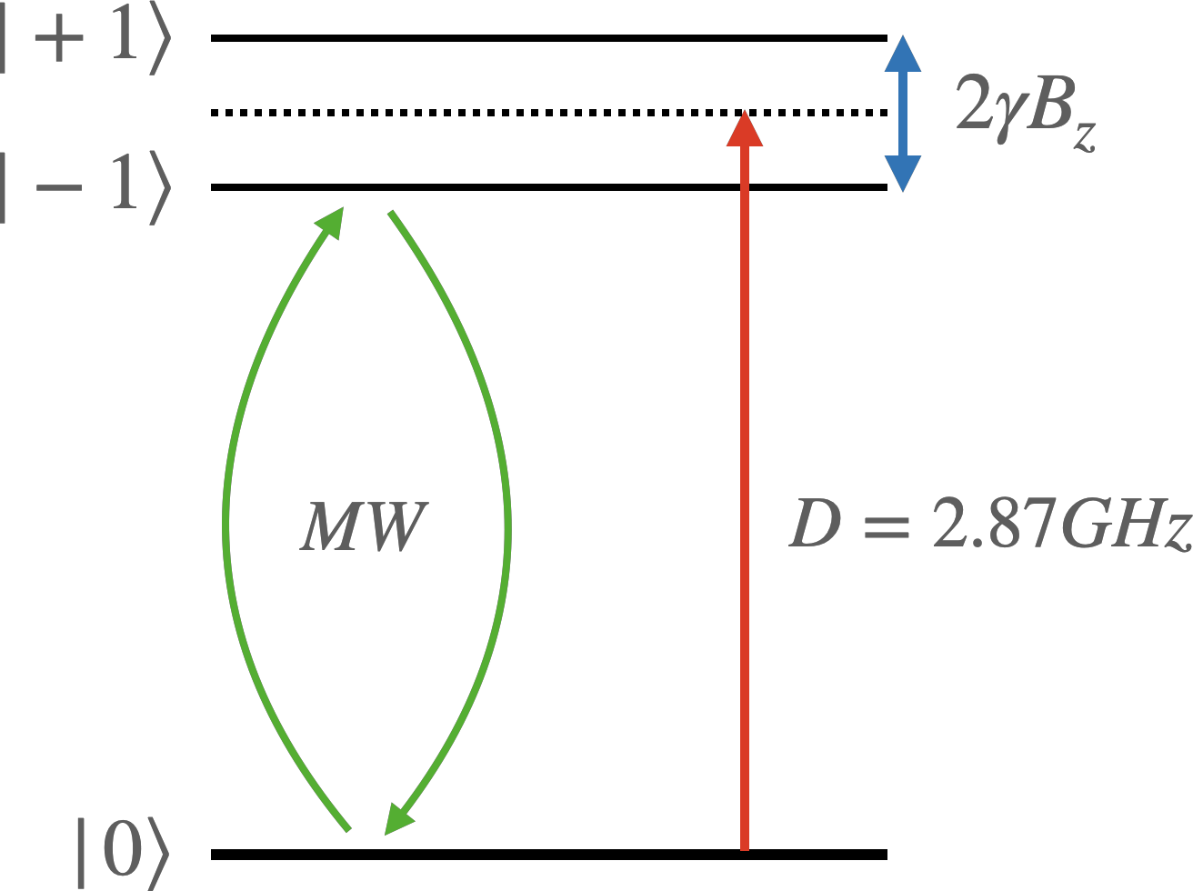
An NV-center is a spin-1 system that froms in a carbon lattice of diamonds if two adjacent carbons are replaced by a nitrogen atom and a vacancy. Without an external field applied, the diamond structure creates a Zero Field Splitting (ZFS). Energy levels corresponding to states and are seperated by MHz.
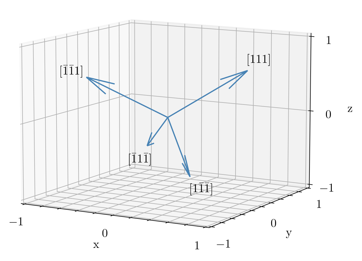
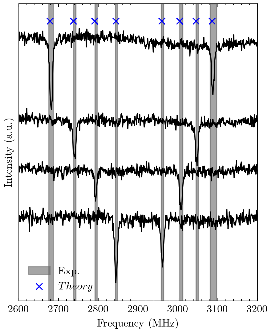
Diamond’s crystalographic axes provide 4 possible orientations of the princial axes of the NV, seperating them into different groups. Different groups have different couplings to a magnetic field, which leads to different energy levels that can be distinguished by optically detected magnetic resonance (ODMR).
In an external magnetic field, the field component along the NV’s princial axis creates an additional energy splitting between and proportional to . This allows selective transitions from the ground state to one of the two exited states by applying a microwave field at resonance frequency. Here we restrict ourselves to transitions to .
The Hamiltonian for an individual NV with microwave drive with Rabi frequency is given by
| (1) |
where the spin operators for are
| (2) |
Applying the unitary to Eq. 1 to transform to a frame co-rotating with the microwave and using rotating-wave approximation (RWA) yields
| (3) |
At resonance frequency, , the microwave drive makes a transition between for the -th NV.
NVs interact with each other via dipole-dipole interaction. We consider a case of strong interaction between NVs and hence ignore nuclear spin. The general definition of dipole-dipole interaction between NV- and NV- is
| (4) |
where are spin operators of NV-, and are the unit vectors connecting the two NVs. Taking into account groups with different princial axes, the dipole-dipole interaction in the rotating frame can be tranformed into an effective Hamiltonian [16],
|
^H_eff,{ij} = {Cdip(^Sx(i)^Sx(j)+ ^Sy(i)^Sy(j)- ^Sz(i)^Sz(j)), same group-Cdip^Sz(i)^Sz(j), different group |
(5) |
where , MHz nm3, . It reduces to and in the case of the same group ().
II.2 QFI and Cramér-Rao bound
According to the Cramér-Rao bound, sensitivity in the estimation of a parameter using quantum probes is bounded by the inverse of the Quantum Fisher Information (QFI), where is the number of independent measurements [25]. Hence, sensitivities can be improved by repeating the measurements or using more probes. For independent probes, we obtain the Standard Quantum Limit (SQL), . However, the QFI can be increased when the probes are highly engtangled. For example, under evolution with a pure Zeeman term, and in the absence of decoherence and dissipation, probes prepared in a GHZ state achieve optimal sensitivity for magnetic field measurement that follows the ”Heisenberg limit” (HL), [26].
Thus, since interactions are necessary for the creation of entanglement, dense NV ensembles harbor the potential for higher sensitivity compared to non-interacting NVs. However, the lack of permutational symmetry leads to the population of other irreducible representations of SU(2) starting from the one with maximum spin, i.e. on average the total spin decays and sensitivity is reduced. Optimal control is therefore necessary to harvest the entanglement from strong interactions for achieving higher sensitivity.
II.3 Tensor network state
Due to the scaling, the interactions within an ensemble of NVs extends beyond the nearest-neighbers and becomes long-range. These all-to-all interactions increase complexity and limit our capability to exactly simulate the system to only a few spins.
To simulate the many-body dynamics for an ensemble of NVs, we represent the quantum state as a tensor network state. In Fig. 2(a) the state of a closed system is decompsed into a 1-dimensional tensor network structure, called Matrix Product State (MPS) [17, 18, 19, 20],
| (6) |
where a matrix . Each in the MPS contains a physical index, representing the local Hilbert space of the NV. The virtual index, or bond index having bond dimensions labels links between two tensors. Physically, the bond dimension contains information about the entanglement entropy between the two parts of the tensor network that the bond connects. Using MPS allows us to compress the bond dimensions and to efficiently represent the ground state in compact, small Hibert spaces.
A similar tensor network structure can be adapted to simulate an open system [27, 28]. To represent an operator we need a Matrix Product Operator (MPO) as given in Fig. 2(b). This MPO, in an orthogonal basis, represents a density operator of the system,
| (7) |
For pure states, this MPO can be contructed by contracting auxiliary indices of two MPS and then combining corresponding physical (bond) indices. Furthermore, we combine the physical indices to create a Matrix Product Density Operator (MPDO) representing a vectorized density operator.
| (8) |
Here, and is combined from two physical indices. The dimension of each resulting index is doubled compared to the MPS. A graphical representation of this process is shown in Fig. 2(c)
II.4 Simulation of dissipative dynamics
We simulate directly, including dissipation, by solving the vectorized master equation
| (9) |
where is the MPDO given by Eq. 8, and is a vectorized Lindblad operator defined as
| (10) |
Note that when , the dynamics are unitary. In this case when MPS is sufficient to simulate the system, utilizing MPDO is unnecessary and computationally more expensive due to the squared memory.
III Results
We model an ensemble of NVs as a 1-dimensional spin-1 chain with long-range interaction. We assume uniform separation, , for nearest neighbor spins. Note that an ensemble with any real-space configuration can be mapped to this model with different interaction strengths. For the very strong interaction regime, this separation is set to be nm while an actual sample in experiment has nm [4]. In our simulations we use the following conditions: i) The amplitude of external magnetic field mT. ii) has a direction calculated from the ODMR data in Fig. 1(c). iii) Uniform Rabi frequency MHz. iv) All NVs belong to the same orientation group parallel to [111]. (v) Time step ns.
III.1 Simulation algorithms in strong interaction regime
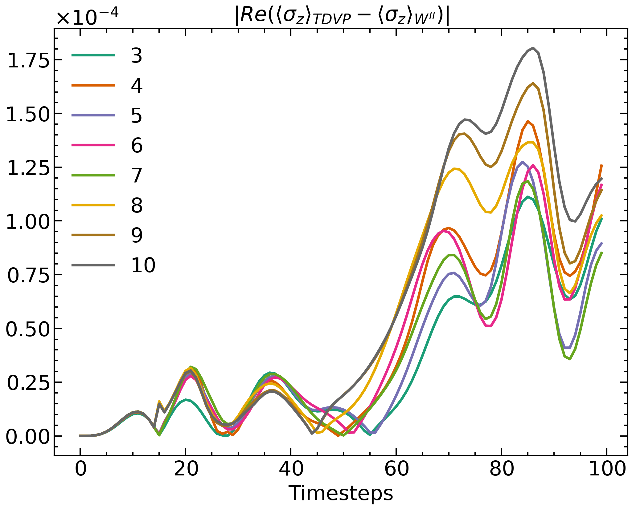
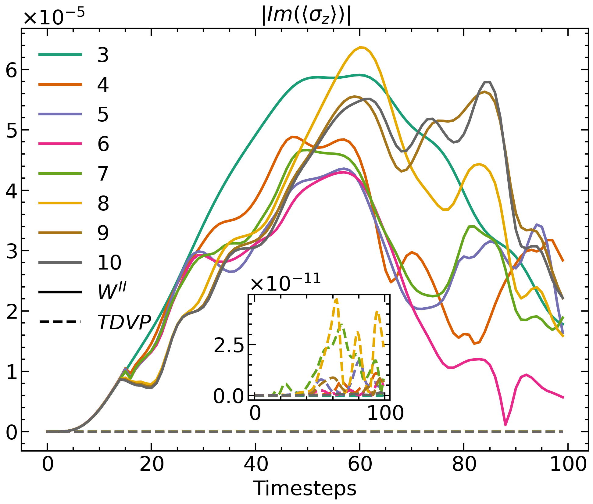
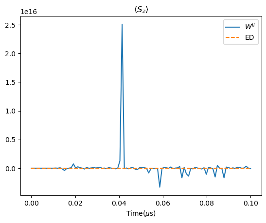
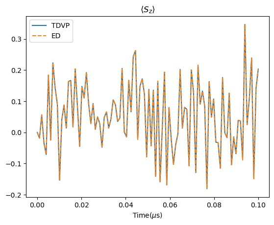
Firstly, we investigate the precision and numerical stability of tensor network algorithms in the very strong interaction regime, for two different algorithms that simulate time-evolution and support the long-range model [29]: i) MPO [30] and ii) time-dependent variational principle (TDVP) [31, 32]. We simulate dynamics of ensembles up to 10 NVs and . Here is a maximum dimension for all bonds. Fig. 3(a) shows that, when nm, both algorithms can simulate the dynamics and have similar expectation values of observables, with only small discrepency. However, the TDVP has significantly smaller errors in the imaginary parts, as shown in Fig. 3(b). When the interaction strength becomes large the also has numerical stability issues and diverging expectation value of a local observable , while the TDVP is still valid compared to exact diagonalization. Fig. 3(c) and Fig. 3(d) are plots of average magnetization of 3 NVs with nm. Hence, we keep the TDVP as the main algorithm for our simulations.
III.2 Dissipative dynamics with finite bond dimension
A major source of error when using MPS/MPDO is truncation error. Keeping finite bond dimensions and truncating when the bond indices exceed introduces an error. This error is given by the square root of the sum of squares of the truncated singular values of all bonds,
| (11) |
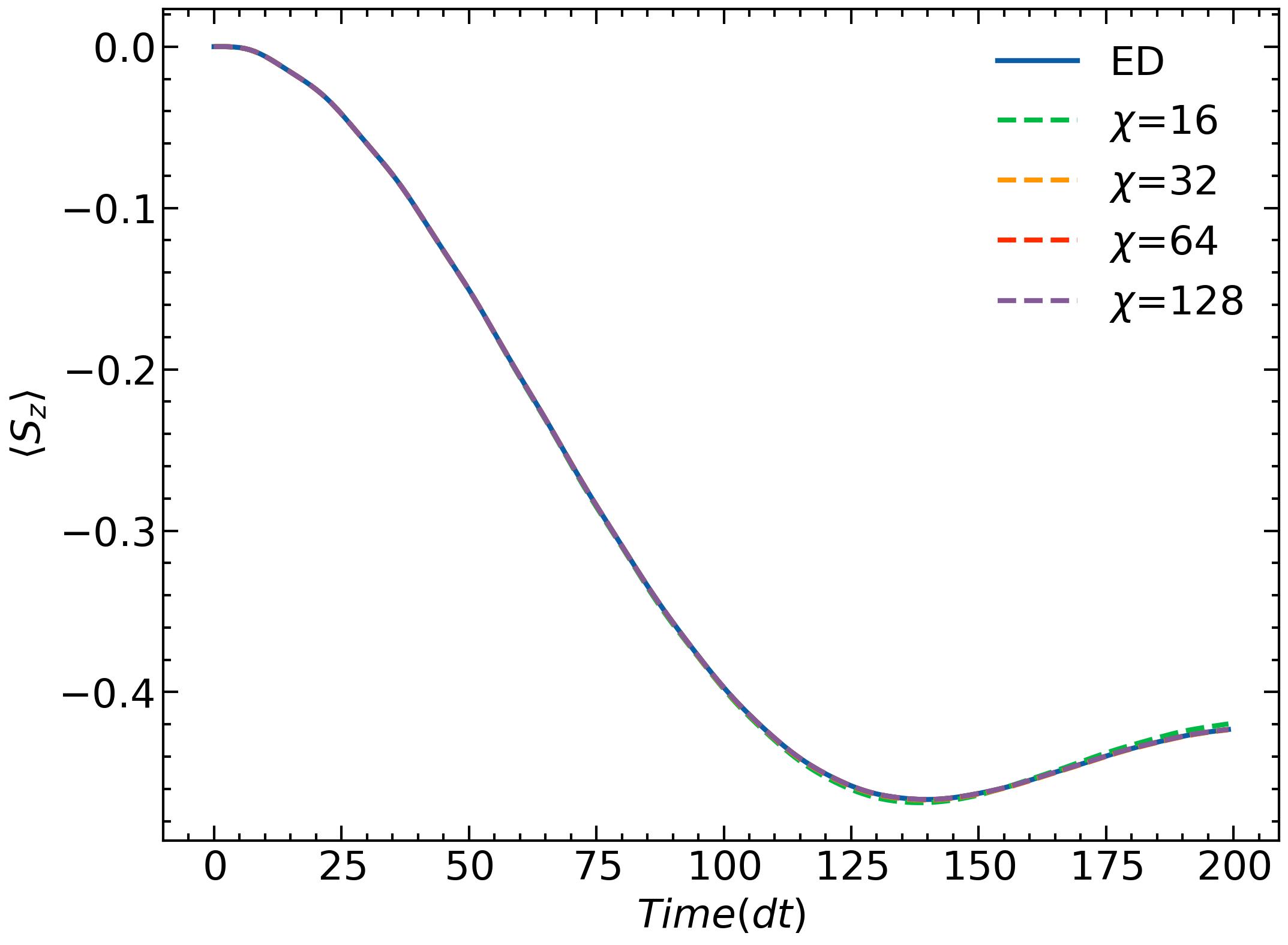
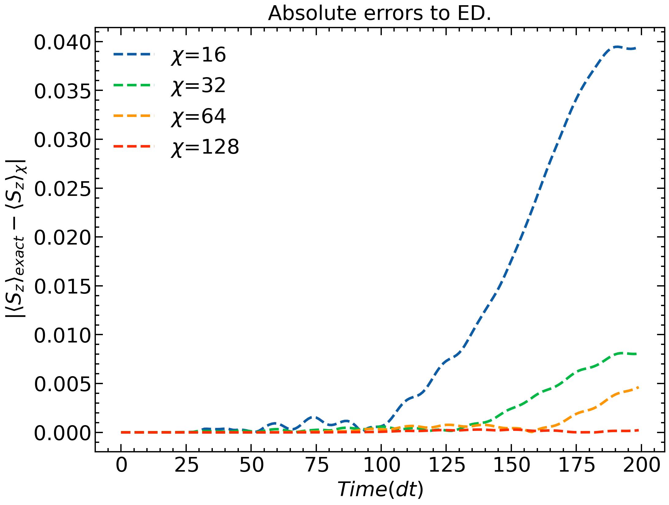
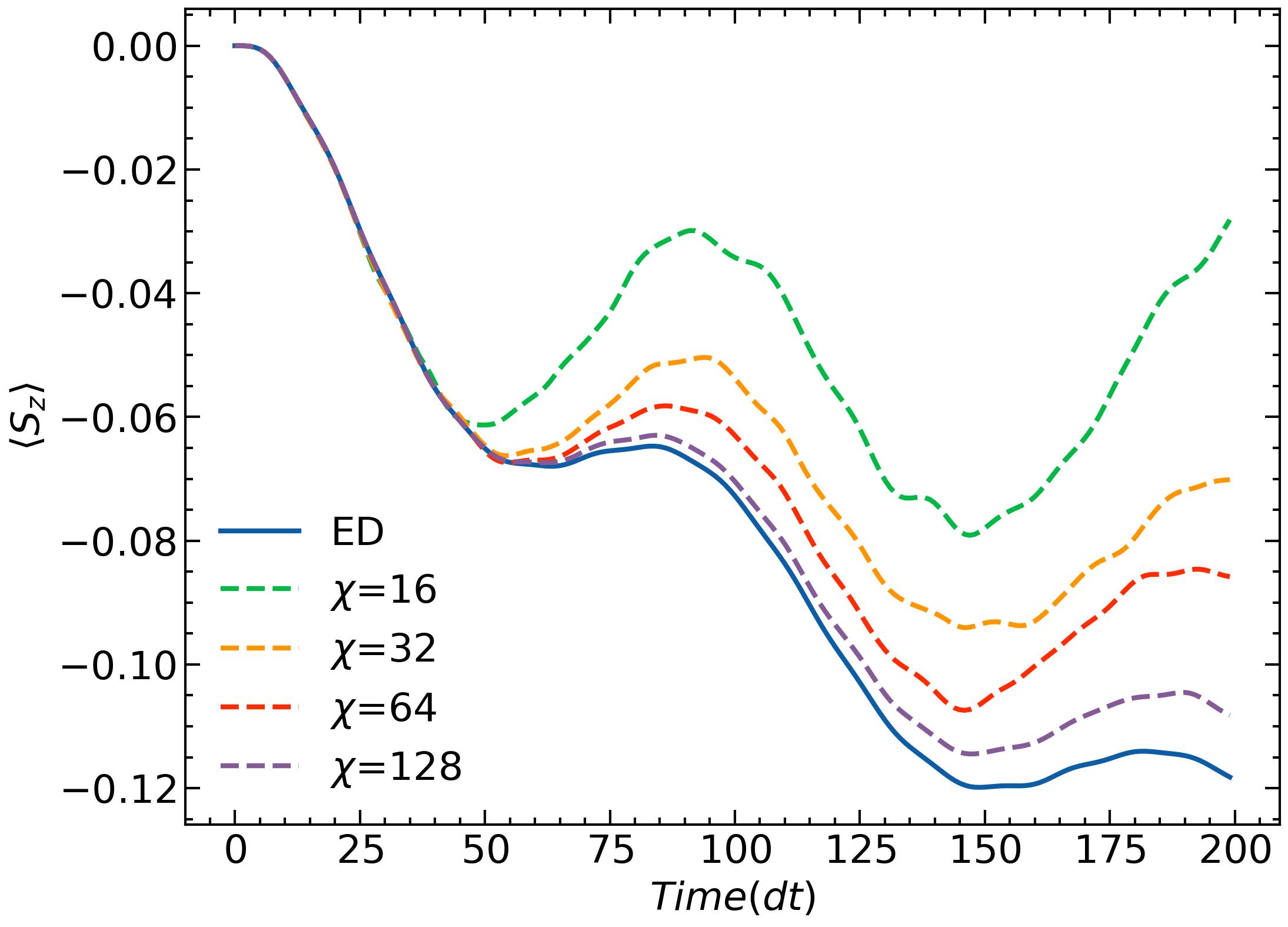
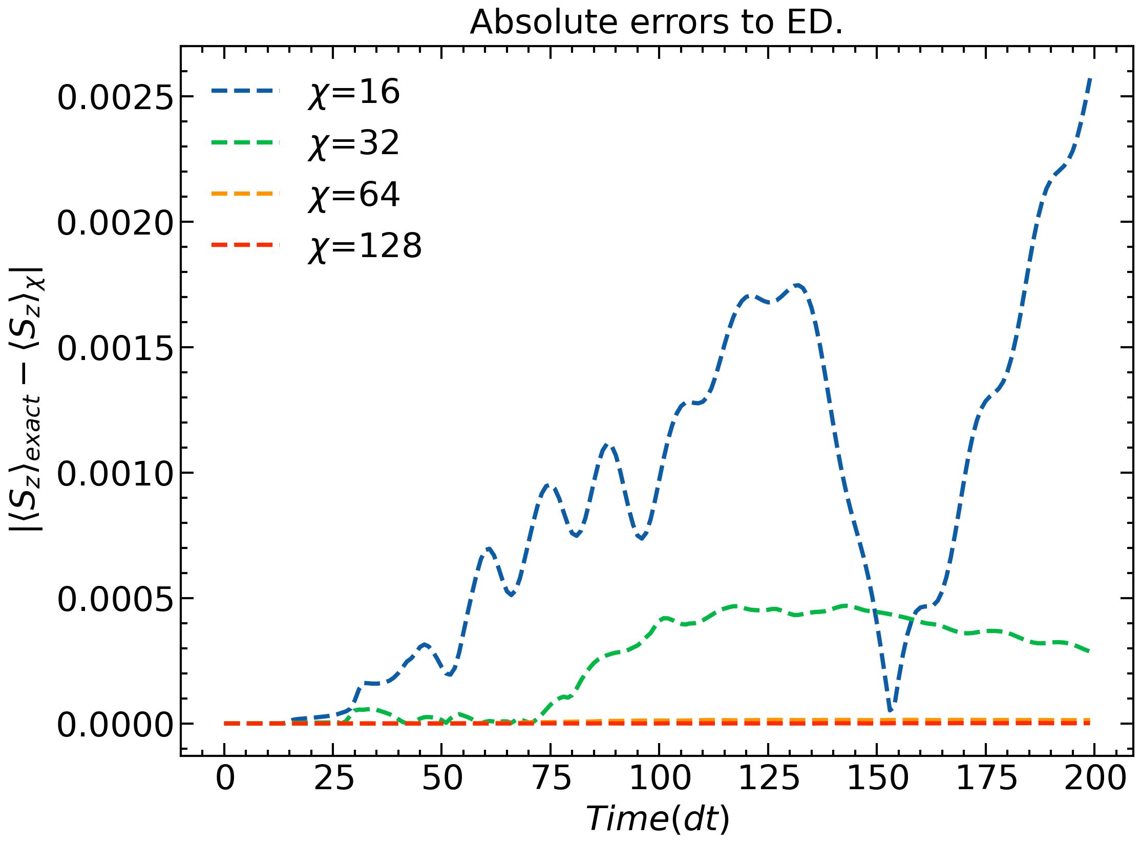
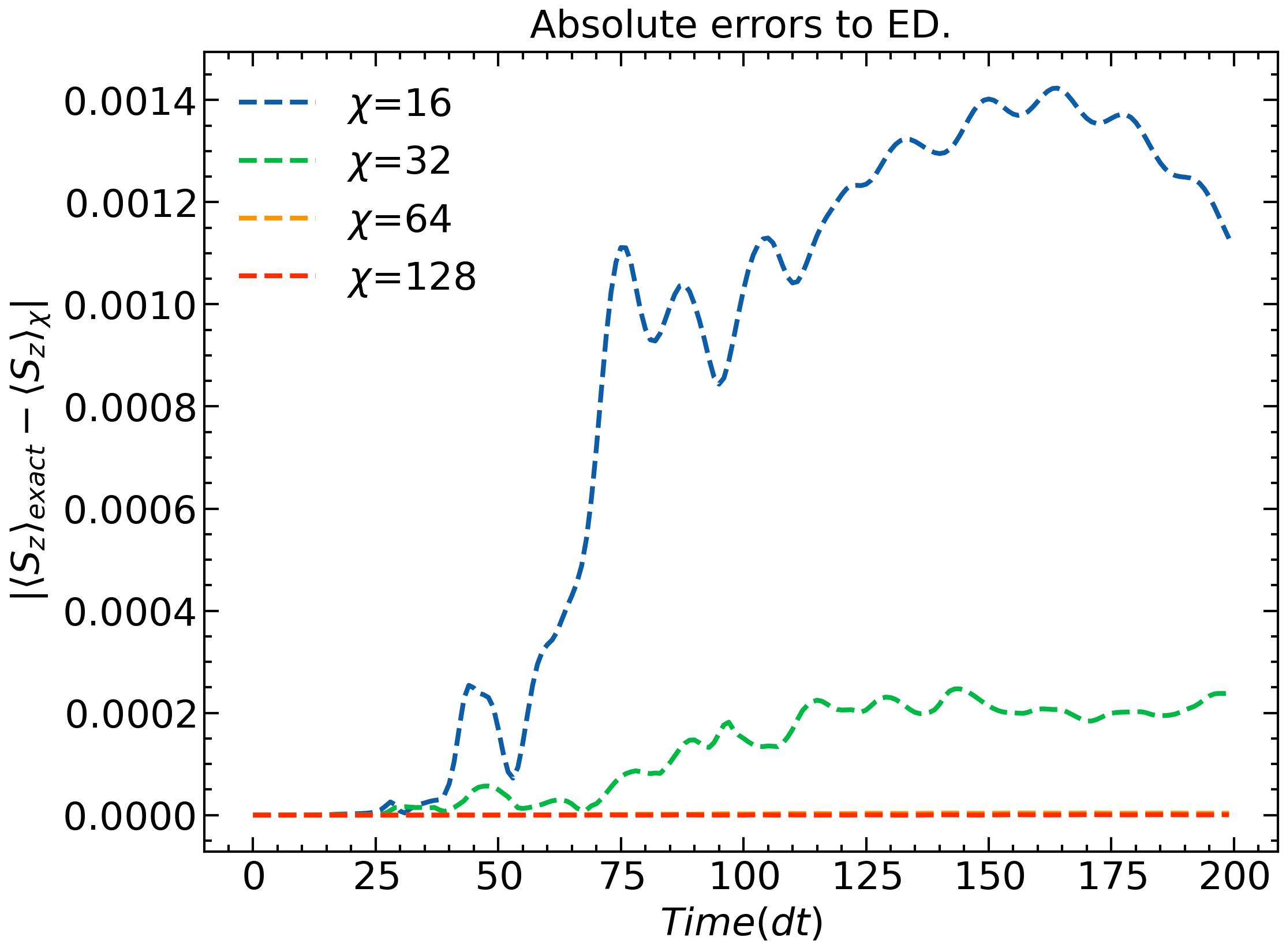
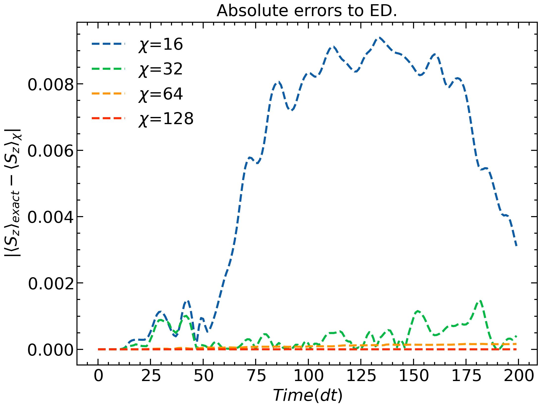
Typically, these errors remain bounded if the state has entanglement that follows an area-law, e.g. when the system has only nearest-neighbor interactions. In such a case, the bond dimension grows with small singular values during the time evolution, allowing the simulation of large systems with small error. However, since we are considering a case of long-range interaction, this argument should not hold. In Fig. 4 and Fig. 5 we plot simulation results for different with nm and nm, compared to a result from exact diagonalization for . We find that stronger interactions introduce bigger errors in bond truncation. The results for smaller only follow the exact calculation as long as entanglement entropy does still not reach ; i.e. up to a certain number of timesteps before diverging and becoming inaccurate due to truncation errors.
These results imply that it requires bigger to capture the dynamics in the presence of long-range, strong interactions, thus less efficiency of the MPS/MPDO method.
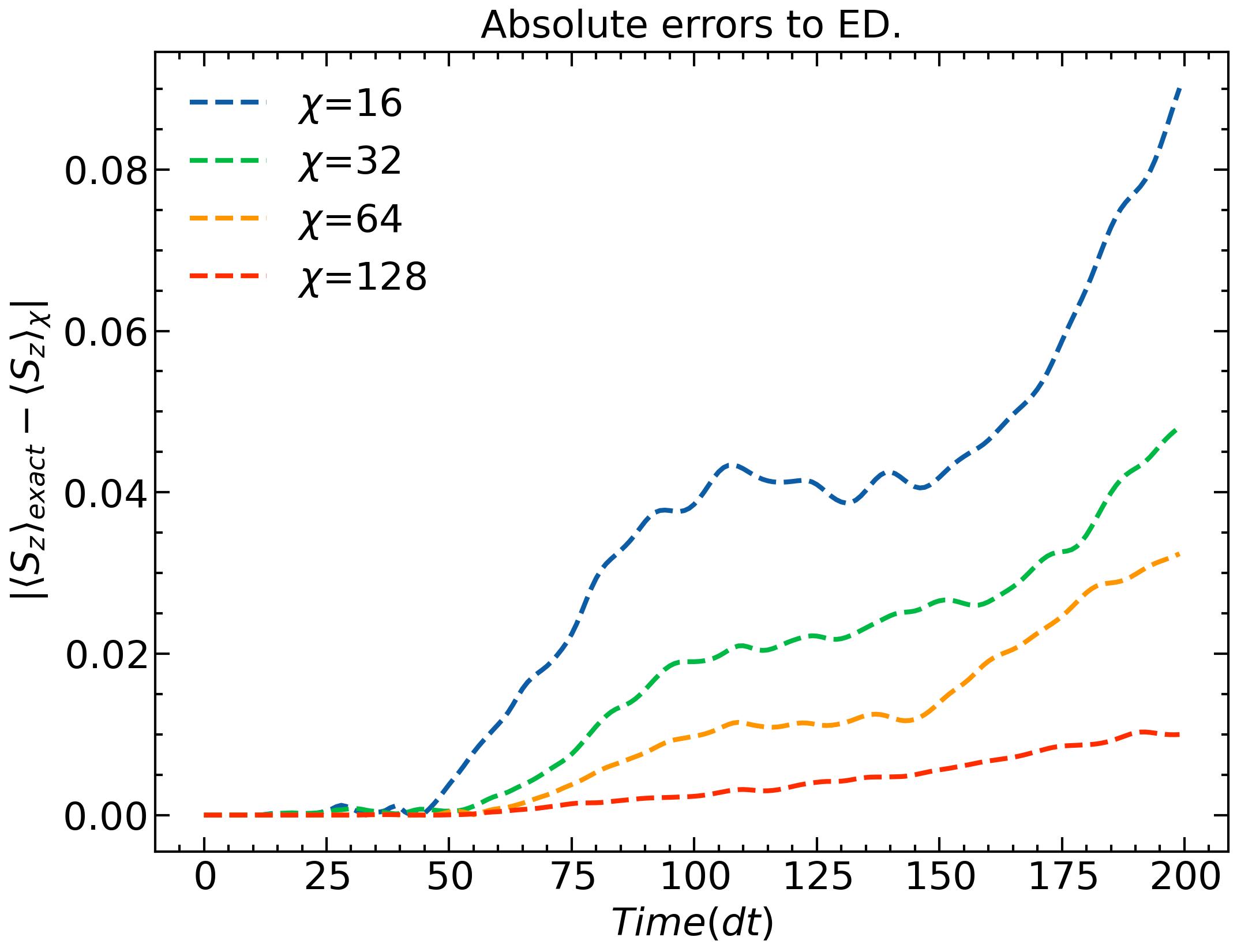
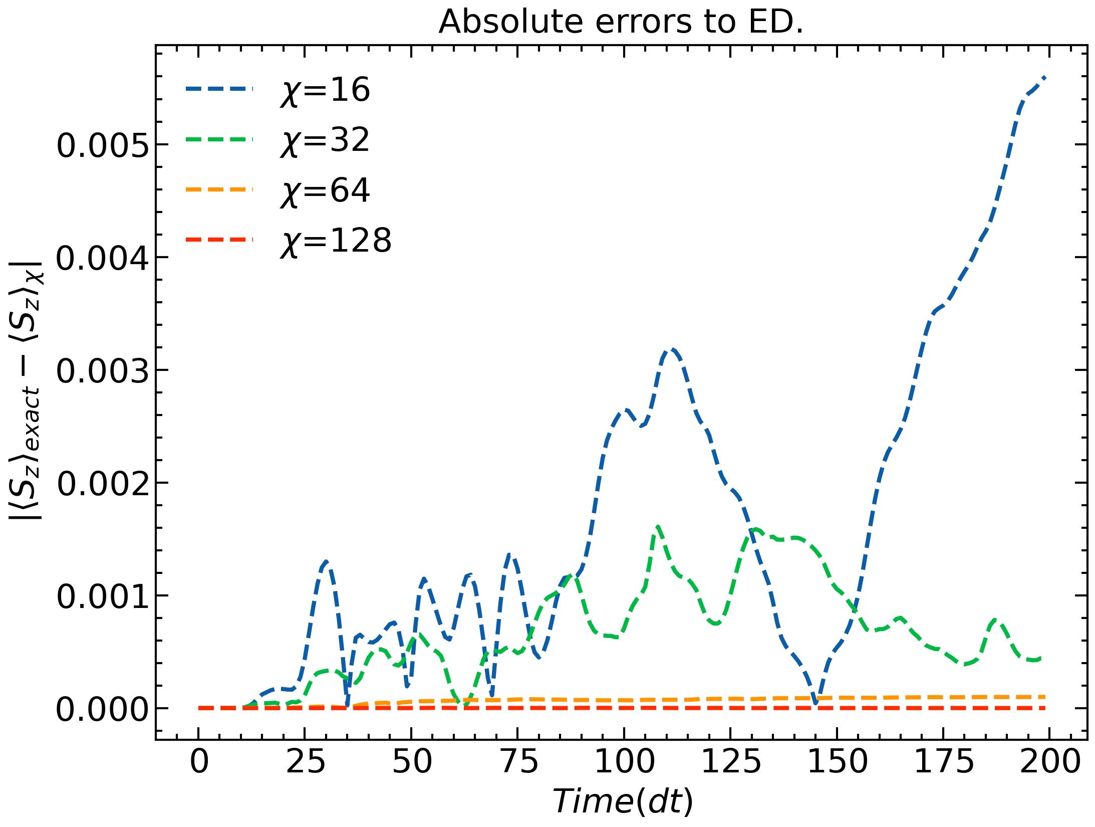
Next, we add dissipation by setting . So each spin has the same dissipation rate. Numerical values of are given in units throughout. For the dissipation operator we choose the dephsasing operator, , relevant, e.g., for magnetic field noise. Fig. 6 shows the absolute errors compared to exact calculations of dissipative dynamics for different . As a result, the discrepency of these dissipative dynamics compared to the exact one is smaller than in the non-dissipative case for the same . When the growth of singular values of bi-partition of the total state across the bond is limited by a larger , bond truncation becomes more effective since it introduces less errors. This demonstrates the interplay between the growth of entanglement entropy due to interactions and dissipation that hinders it.
To understand quantitatively how stronger interactions induce entanglement entropy during time-evolution, we calculate the Operator Entanglement Entropy (opEE) of the reduced density matrix determined by cutting the system into two halves at the middle bond and tracing out the other half. We use the von Neuman entropy defined as [33]
| (12) |
where are singular values of the cut bond with bond dimension for the vectorized operator. Here the are squared because they are singular values of a vectorized operator . Note that in general opEE does not give a direct measure of entanglement for mixed states. The opEE for a pure state is twice the value of its standard entanglement entropy, , when [34]. Yet, the opEE provides insight into how well the state can be approximated by an MPDO, indicating simulation errors from a truncation [35].
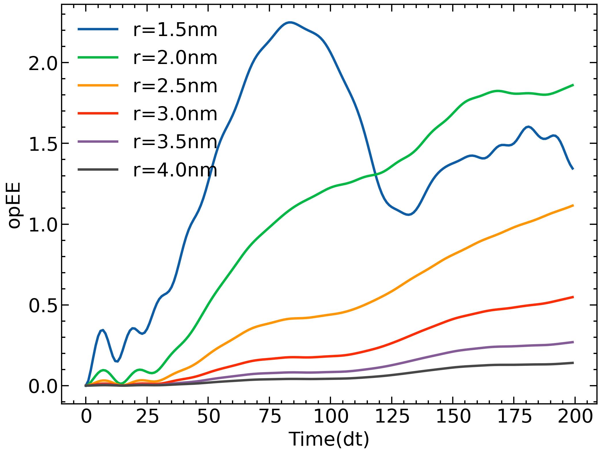
After time-evolution, the middle bond index which is the bond that equally separates the MPDO into two halves has the largest dimension. Fig. 7(d) shows the time evolution of opEE calculated from cutting the middle bond. The opEE growth as function of time is accelerated as interactions become stronger. This agrees with results of larger errors from truncation shown earlier. Except at very strong interaction, i.e. for nm, opEE grows at the beginning and saturates rapidly. This is because the interaction strengths are comparable to the Rabi frequency . However, we observe that this can be altered by increasing .
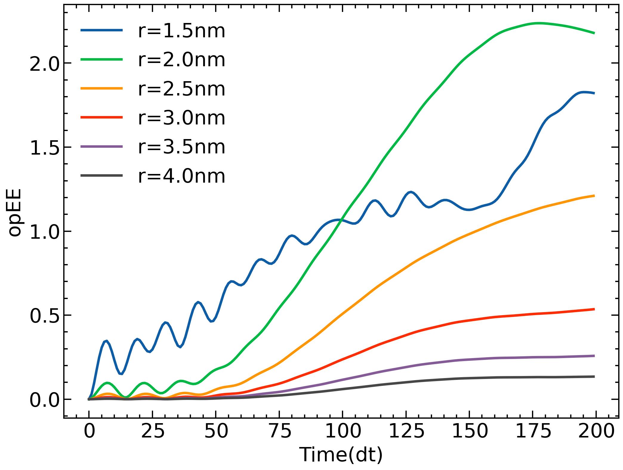
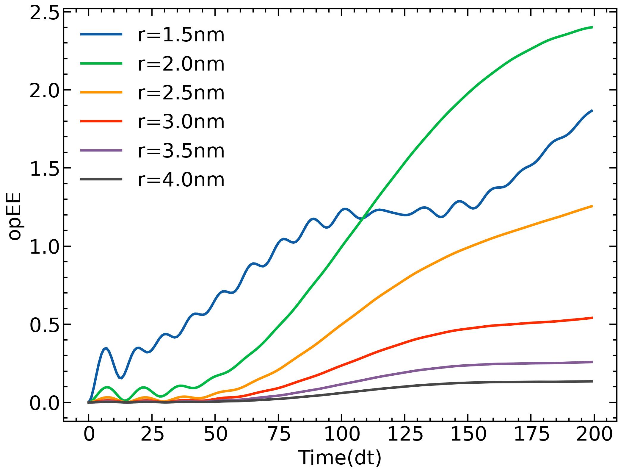
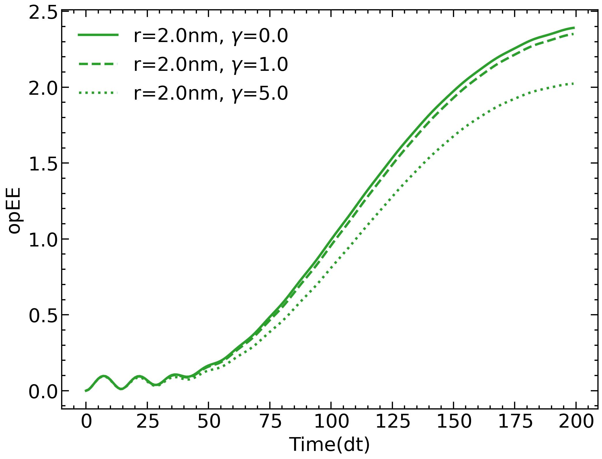
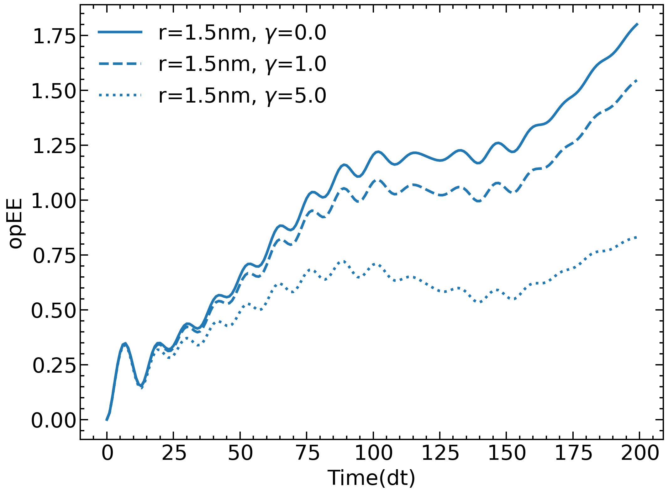
dissipation suppresses generation of opEE.
III.3 Dynamics of QFI
To quantify the sensitivity of the ensemble of interacting NVs to a uniform magnetic field , we compute the Quantum Fisher Information of the mixed state during time evolution. We use the tensor network approach for calculating QFI as in [36]. Note that, unlike in the original work [36], we only optimize the symmetric logarithmic derivative (SLD) but not the input state . In short, we iteratively search for the SLD that satisfies a definition of QFI:
| (13) |
At the beginning, we randomly create the MPO approximation of an SLD, , given by
| (14) |
Here is a Hermitian matrix. In searching for an optimal we locally update by sweeping from to and back to again until has converged. For example, when updating , all other tensors are fixed and combined. Then after contractions, Eq. 13 becomes
| (15) |
Here, and are a vector and a matrix resulting from contracting the fixed tensors and combining the un-contracted indices. The diagrammatic explanation can be found on page 8 of [36]. Taking the derivative with respect to , , Eq. 15 yields . A solution to this equation provides a local extremum for the QFI. Since this local update approach tends to get stuck at local extrema, several repetitions with different initial are needed and can be computational expensive for large .
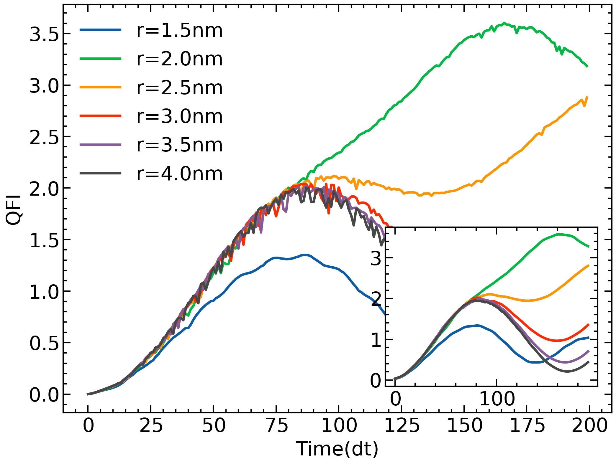
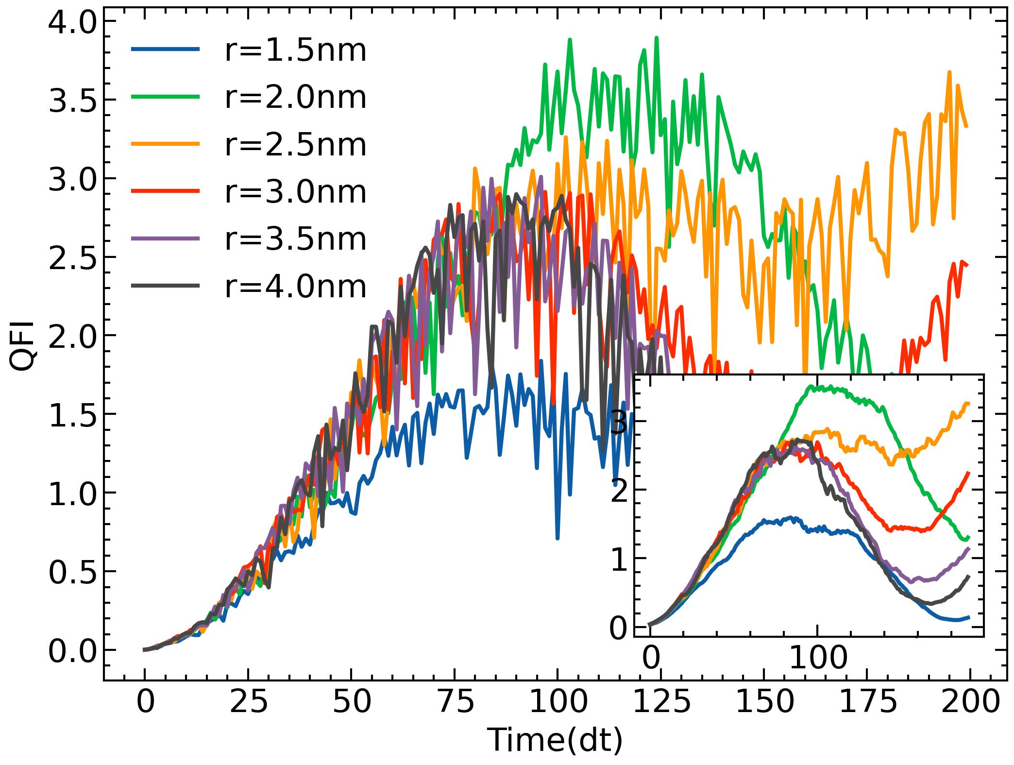
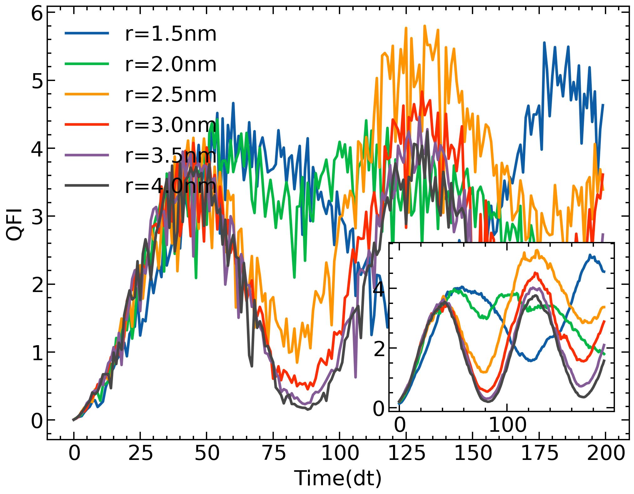
Fig. 8 shows the dynamics of the QFI for a non-dissipative system with small size and different . At each time step, we find the optimal SLD from 10 independent realizations and select the one with the largest QFI. Furthermore, we utilize the optimal SLD obtained from the previous time step as the initialization for the current time step. Based on our experience, although not guaranteed, implementing such a strategy can lead to a smoother result for the QFI.
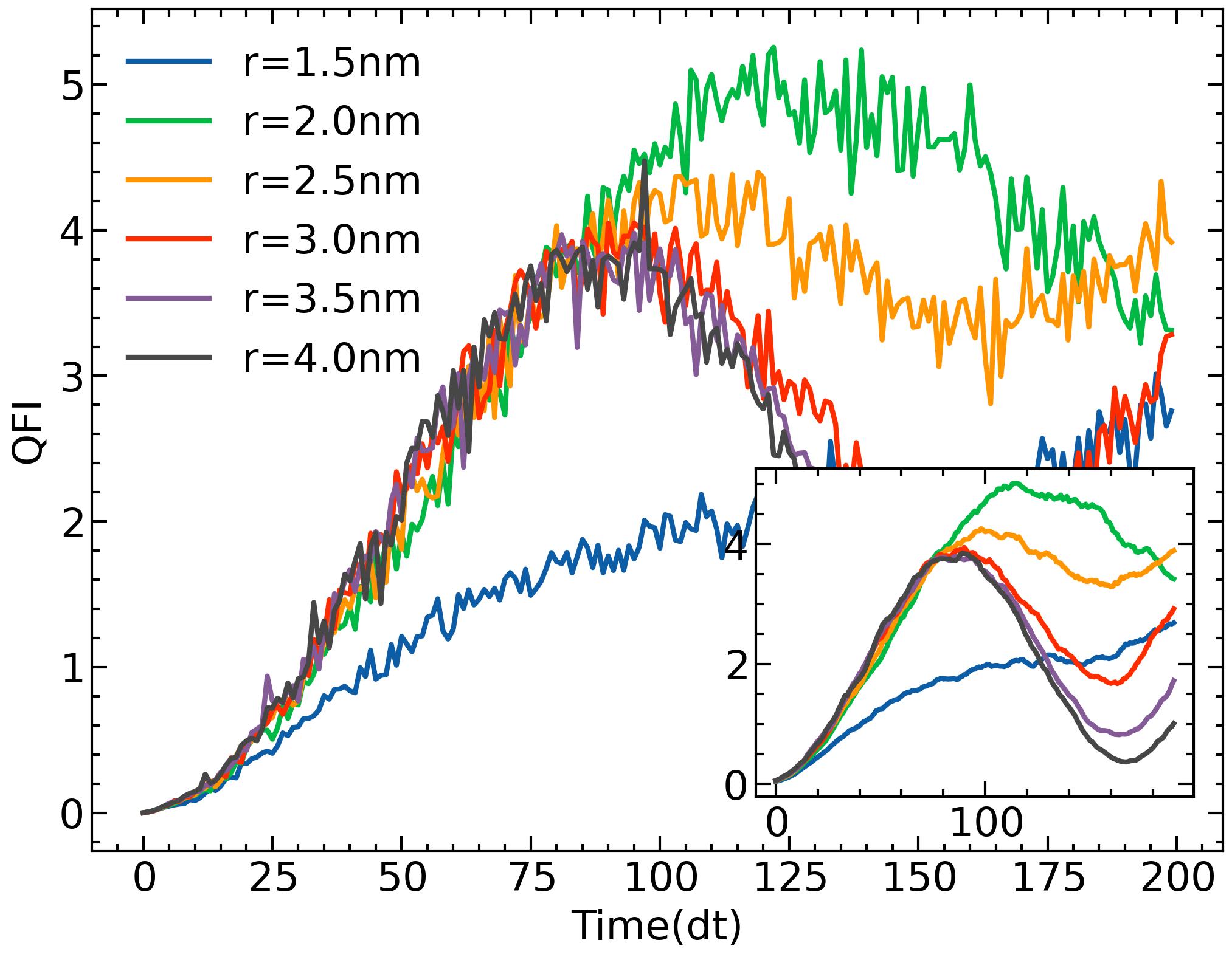
According to the plots, the QFI of nm nearly reaches values of non-interacting probes, denoted as . The QFI increases if the interactions are stonger, especially when nm, leading to a QFI that can be greater than . This suggests that the sensitivity for the probes is enhanced by the entanglement that is created by interaction. Still, as for opEE, the QFI remains relatively small when nm, i.e. for very strong interaction. We find that this is due to an interaction strength of the nearest NV pairs ( MHz) that becomes substantially larger than the Rabi frequency ( MHz). As shown Fig. 9, the QFI can be further increased also for nm by increasing the Rabi frequency.
IV Conclusion
An ensemble of NV centers is a promising quantum metrology platform. While adding more independent spins improves the sensitivity, the probe can in principle also reach greater sensitivity due to entanglement created by interactions. Also, having a dense ensemble means that the total size of the probe can be smaller, resulting in better spatial resolution. However, without external control of the entanglement and the states generated, strong dipole-dipole interactions due to small separations between NV centers within a dense ensemble are usually detrimental for the sensitivity as they lead to a rapid decay of the total spin.
To investigate a strongly interacting NVs system, we simulated the master equation with dissipation using MPDO. We benchmarked tensor network algorithms for time evolution with a long-range interaction model. We found the algorithm to have bigger imaginary errors and to be less stable in a very small separation regime than TDVP. Then, for small NV separations, we investigated the effect of finite maximum bond dimensions on the simulation accuracy. We determined the accuracy by comparing the obtained states to those from exact diagonalization. Stronger interactions result in larger errors, suggesting the need for larger bonds. For dissipative dynamics, we found higher accuracy, which shows suppression of operator entanglement entropy growth. These results indicate that the tensor network method can be suitable for simulating an open system.
For applications in quantum sensing, we used the approach of locally optimizing approximations of the SLD to obtain the quantum Fisher information. The QFI of driven ensembles shows that strong interaction can create entanglement-enhanced sensitivity compared to independent spins.
Finally, we observed that the boost in sensitivity can diminish when the interaction becomes significantly larger than the Rabi frequency. In this situation, it is necessary to utilize microwaves with higher frequencies for driving in order to increase the sensitivity.
Appendix A Pure state entanglement entropy for a vector and an operator.
Any pure state has a Schmidt decomposition with Schmidt coefficients and . Then we can define the reduced density matrix for a bipartite system by partial trace over the other parts: and The density operator of the total system reads . The entanglement entropy for reduced density operators is defined as
| (16) |
where . To find the operator entanglement entropy (opEE), we vectorize ,
| (17) | ||||
| (18) |
Here and . The super density operator, denoted by , can be created using an outer product:
| (19) | ||||
| (20) |
Similar to , we can also have ; e.g. Then we can find the opEE,
| (21) | ||||
| (22) | ||||
| (23) | ||||
| (24) | ||||
| (25) | ||||
| (26) |
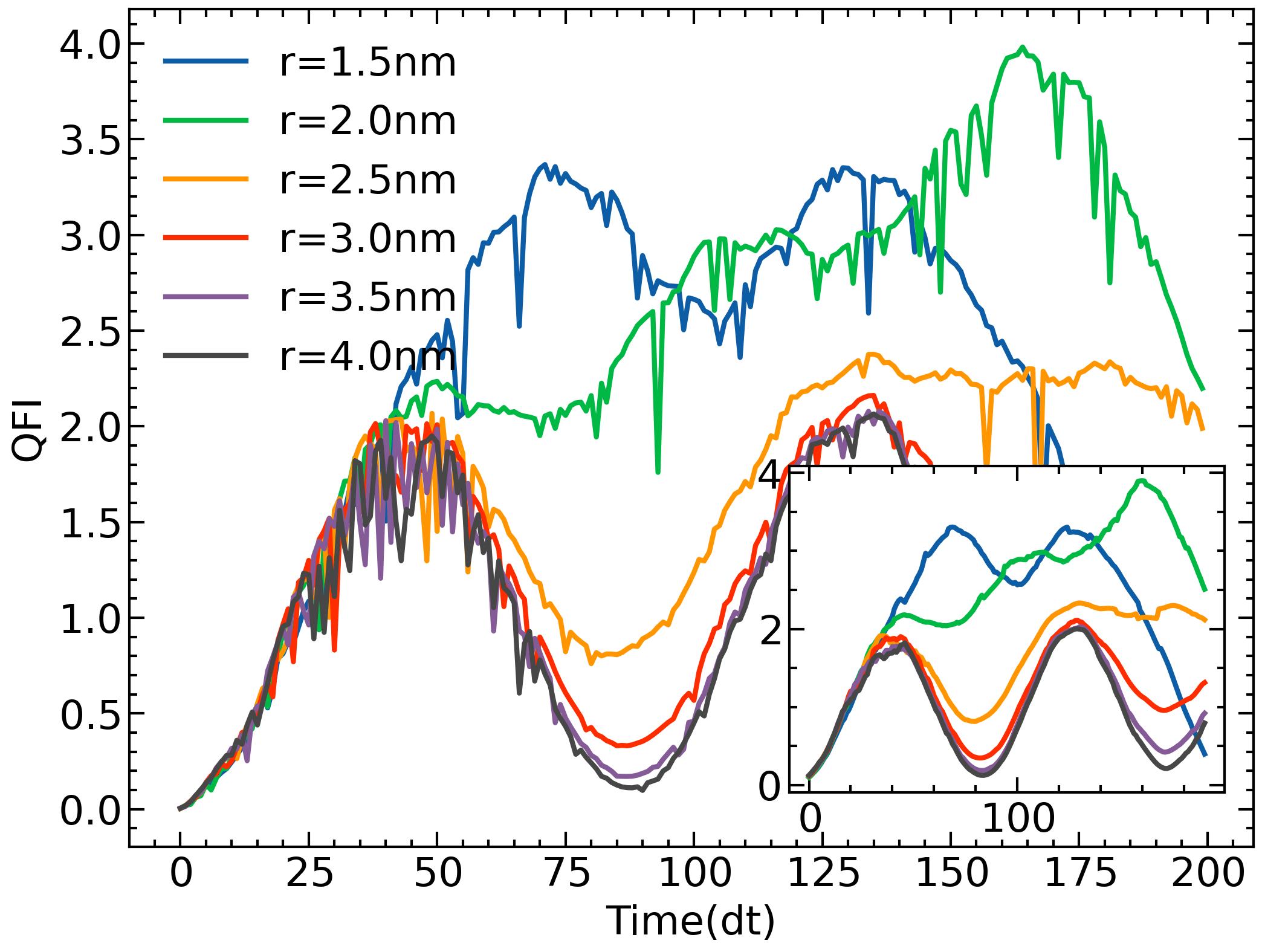
Appendix B opEE for Rabi frequency
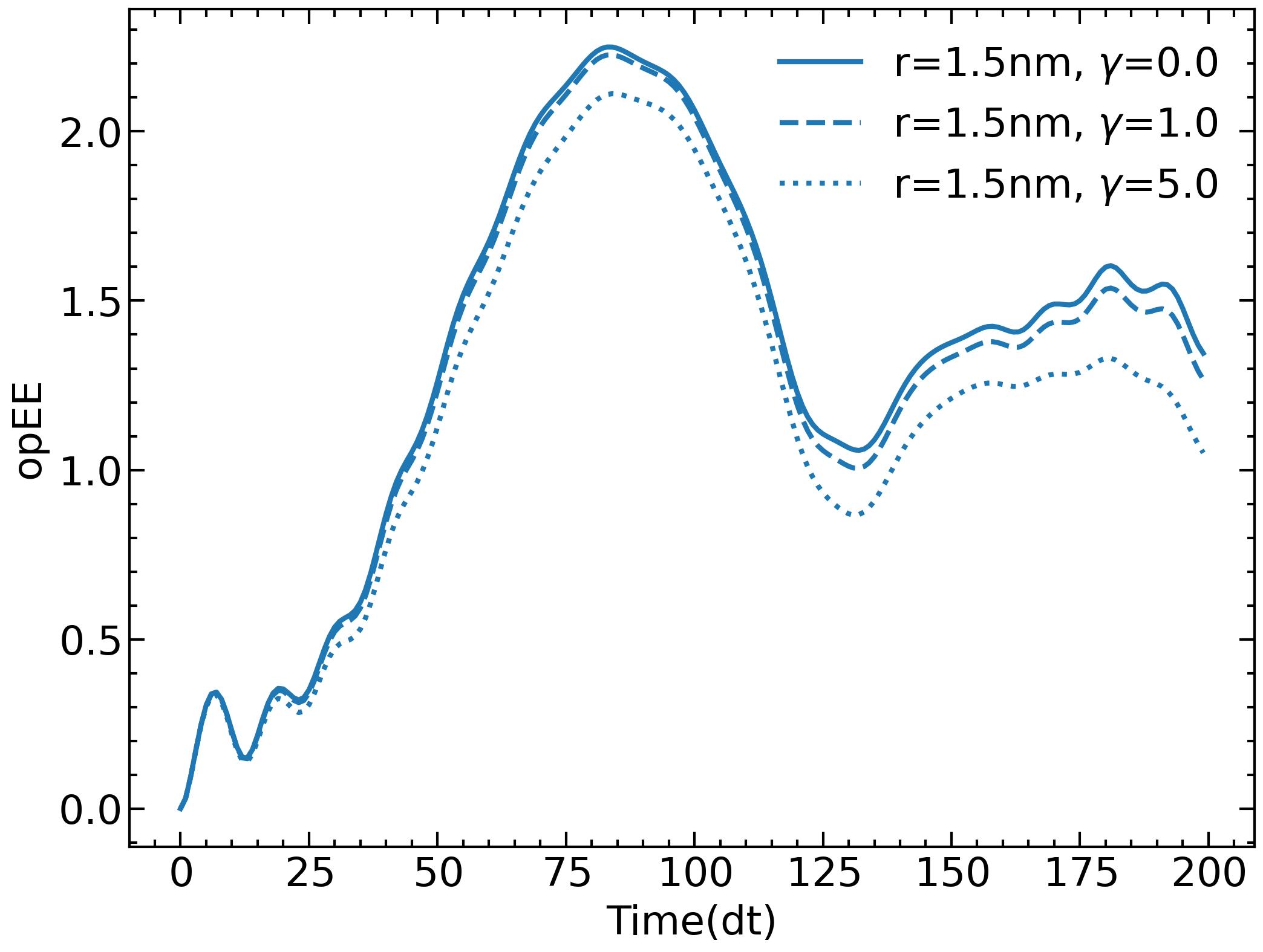
The operator entanglement entropy when the Rabi frequency is doubled from MHz, hence MHz.
Acknowledgements.
This work was supported by the Baden Württemberg Stiftung, project CDINQUA. Tensor network codes are modified and implemented algorithms from TenPy [37].References
- Taylor et al. [2008] J. M. Taylor, P. Cappellaro, L. Childress, L. Jiang, D. Budker, P. R. Hemmer, A. Yacoby, R. Walsworth, and M. D. Lukin, Nature Phys 4, 810 (2008), publisher: Nature Publishing Group.
- Welter et al. [2022] P. Welter, J. Rhensius, A. Morales, M. S. Wörnle, C. H. Lambert, G. Puebla-Hellmann, P. Gambardella, and C. L. Degen, Applied Physics Letters 120, 074003 (2022).
- Dwyer et al. [2022] B. L. Dwyer, L. V. Rodgers, E. K. Urbach, D. Bluvstein, S. Sangtawesin, H. Zhou, Y. Nassab, M. Fitzpatrick, Z. Yuan, K. De Greve, E. L. Peterson, H. Knowles, T. Sumarac, J.-P. Chou, A. Gali, V. Dobrovitski, M. D. Lukin, and N. P. de Leon, PRX Quantum 3, 040328 (2022), publisher: American Physical Society.
- Haruyama et al. [2019] M. Haruyama, S. Onoda, T. Higuchi, W. Kada, A. Chiba, Y. Hirano, T. Teraji, R. Igarashi, S. Kawai, H. Kawarada, Y. Ishii, R. Fukuda, T. Tanii, J. Isoya, T. Ohshima, and O. Hanaizumi, Nature Communications 2019 10:1 10, 1 (2019), publisher: Nature Publishing Group.
- Balasubramanian et al. [2019] P. Balasubramanian, C. Osterkamp, Y. Chen, X. Chen, T. Teraji, E. Wu, B. Naydenov, and F. Jelezko, Nano Lett. 19, 6681 (2019), publisher: American Chemical Society.
- Zheng et al. [2019] H. Zheng, J. Xu, G. Z. Iwata, T. Lenz, J. Michl, B. Yavkin, K. Nakamura, H. Sumiya, T. Ohshima, J. Isoya, J. Wrachtrup, A. Wickenbrock, and D. Budker, Phys. Rev. Appl. 11, 064068 (2019), publisher: American Physical Society.
- Wang et al. [2022] C. Wang, Q. Liu, Y. Hu, F. Xie, K. Krishna, N. Wang, L. Wang, Y. Wang, K. C. Toussaint Jr, J. Cheng, H. Chen, and Z. Wu, Realization of high-dynamic-range broadband magnetic-field sensing with ensemble nitrogen-vacancy centers in diamond (2022), arXiv:2209.11360 [quant-ph].
- Zhou et al. [2020] H. Zhou, J. Choi, S. Choi, R. Landig, A. M. Douglas, J. Isoya, F. Jelezko, S. Onoda, H. Sumiya, P. Cappellaro, H. S. Knowles, H. Park, and M. D. Lukin, Phys. Rev. X 10, 031003 (2020), publisher: American Physical Society.
- Bauch et al. [2020] E. Bauch, S. Singh, J. Lee, C. A. Hart, J. M. Schloss, M. J. Turner, J. F. Barry, L. M. Pham, N. Bar-Gill, S. F. Yelin, and R. L. Walsworth, PHYSICAL REVIEW B 102, 134210 (2020).
- Farfurnik et al. [2018] D. Farfurnik, Y. Horowicz, and N. Bar-Gill, Phys. Rev. A 98, 033409 (2018).
- Osterkamp et al. [2019] C. Osterkamp, M. Mangold, J. Lang, P. Balasubramanian, T. Teraji, B. Naydenov, and F. Jelezko, Sci Rep 9, 5786 (2019), publisher: Nature Publishing Group.
- Sandvik [2010] A. W. Sandvik, Phys. Rev. Lett. 104, 137204 (2010).
- Schiffer et al. [2019] S. Schiffer, J. Wang, X.-J. Liu, and H. Hu, Phys. Rev. A 100, 063619 (2019), publisher: American Physical Society.
- Cheng [2023] C. Cheng, Phys. Rev. B 108, 155113 (2023).
- Essink [2018] S. Essink, Boundary-Driven XXZ Spin-1/2 Chain, Ph.D. thesis, Universität Bonn, Bonn (2018).
- Kucsko et al. [2018] G. Kucsko, S. Choi, J. Choi, P. Maurer, H. Zhou, R. Landig, H. Sumiya, S. Onoda, J. Isoya, F. Jelezko, E. Demler, N. Yao, and M. Lukin, Phys. Rev. Lett. 121, 023601 (2018).
- Vidal [2003] G. Vidal, Phys. Rev. Lett. 91, 147902 (2003), publisher: American Physical Society.
- Perez-Garcia et al. [2007] D. Perez-Garcia, F. Verstraete, M. M. Wolf, and J. I. Cirac, Quantum Info. Comput. 7, 401–430 (2007).
- Schollwöck [2011] U. Schollwöck, Annals of Physics January 2011 Special Issue, 326, 96 (2011).
- Orús [2014] R. Orús, Annals of Physics 349, 117 (2014).
- Jarzyna and Demkowicz-Dobrzański [2013] M. Jarzyna and R. Demkowicz-Dobrzański, Phys. Rev. Lett. 110, 240405 (2013).
- Finsterhölzl et al. [2020] R. Finsterhölzl, M. Katzer, A. Knorr, and A. Carmele, Entropy 22, 984 (2020), number: 9 Publisher: Multidisciplinary Digital Publishing Institute.
- Schlimgen et al. [2022] A. W. Schlimgen, K. Head-Marsden, L. M. Sager, P. Narang, and D. A. Mazziotti, Phys. Rev. Research 4, 023216 (2022).
- Fux et al. [2023] G. E. Fux, D. Kilda, B. W. Lovett, and J. Keeling, Phys. Rev. Research 5, 033078 (2023).
- Paris [2009] M. G. A. Paris, Int. J. Quantum Inform. 07, 125 (2009), publisher: World Scientific Publishing Co.
- Giovannetti et al. [2004] V. Giovannetti, S. Lloyd, and L. Maccone, Science 306, 1330 (2004), publisher: American Association for the Advancement of Science.
- Weimer et al. [2021] H. Weimer, A. Kshetrimayum, and R. Orús, Rev. Mod. Phys. 93, 015008 (2021).
- Jaschke et al. [2018] D. Jaschke, S. Montangero, and L. D. Carr, Quantum Science and Technology 4, 013001 (2018).
- Paeckel et al. [2019] S. Paeckel, T. Köhler, A. Swoboda, S. R. Manmana, U. Schollwöck, and C. Hubig, Annals of Physics 411, 167998 (2019).
- Zaletel et al. [2015] M. P. Zaletel, R. S. K. Mong, C. Karrasch, J. E. Moore, and F. Pollmann, Phys. Rev. B 91, 165112 (2015).
- Haegeman et al. [2016] J. Haegeman, C. Lubich, I. Oseledets, B. Vandereycken, and F. Verstraete, Phys. Rev. B 94, 165116 (2016), publisher: American Physical Society.
- Hubig et al. [2018] C. Hubig, J. Haegeman, and U. Schollwöck, Phys. Rev. B 97, 045125 (2018), publisher: American Physical Society.
- Murciano et al. [2024] S. Murciano, J. Dubail, and P. Calabrese, J. Phys. A: Math. Theor. 57, 145002 (2024), publisher: IOP Publishing.
- Preisser Beltrán [2023] G. J. Preisser Beltrán, Numerical studies of entanglement dynamics in open spin systems, These de doctorat, Strasbourg (2023).
- Preisser et al. [2023] G. Preisser, D. Wellnitz, T. Botzung, and J. Schachenmayer, Phys. Rev. A 108, 012616 (2023).
- Chabuda et al. [2020] K. Chabuda, J. Dziarmaga, T. J. Osborne, and R. Demkowicz-Dobrzański, Nat Commun 11, 250 (2020), number: 1 Publisher: Nature Publishing Group.
- Hauschild and Pollmann [2018] J. Hauschild and F. Pollmann, SciPost Phys. Lect. Notes , 5 (2018).