Resource Leveling: Complexity of a UET two-processor scheduling variant and related problems
Abstract
This paper mainly focuses on a resource leveling variant of a two-processor scheduling problem. The latter problem is to schedule a set of dependent UET jobs on two identical processors with minimum makespan. It is known to be polynomial-time solvable.
In the variant we consider, the resource constraint on processors is relaxed and the objective is no longer to minimize makespan. Instead, a deadline is imposed on the makespan and the objective is to minimize the total resource use exceeding a threshold resource level of two. This resource leveling criterion is known as the total overload cost. Sophisticated matching arguments allow us to provide a polynomial algorithm computing the optimal solution as a function of the makespan deadline. It extends a solving method from the literature for the two-processor scheduling problem.
Moreover, the complexity of related resource leveling problems sharing the same objective is studied. These results lead to polynomial or pseudo-polynomial algorithms or -hardness proofs, allowing for an interesting comparison with classical machine scheduling problems.
Keywords: Scheduling, resource leveling, complexity, matchings
1 Introduction
Most project scheduling applications involve renewable resources such as machines or workers. A natural assumption is to consider that the amount of such resources is limited, as in the widely studied Resource Constrained Project Scheduling Problem (RCPSP). In many cases however, the resource capacity can be exceeded if needed, yet at a significant cost, by hiring additional workforce for instance. The field of scheduling known as resource leveling aims at modelling such costs: while resource capacities are not a hard constraint, the objective function is chosen to penalize resource overspending or other irregularities in resource use.
Related works
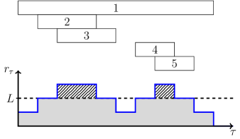
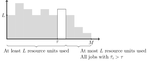
Resource leveling is a well studied topic in recent literature, as a variant of the RCPSP – see Hartmann and Briskorn [2022] for a survey. Among the various leveling objective functions that are proposed, a very natural one is the total overload cost, used in Rieck et al. [2012], Rieck and Zimmermann [2015], Bianco et al. [2016], Atan and Eren [2018], Verbeeck et al. [2017]. The total overload cost, that is the resource use exceeding a given level, is suitable for modelling the cost of mobilizing supplementary resource capacity, the level representing a base capacity that should ideally not be exceeded. Considering a single resource of level and denoting the resource request at time step , the function writes (see the hatched part in Figure 1). Other notable examples of leveling objective functions introduced in the literature are weighted square capacities [Christodoulou et al., 2015, Ponz-Tienda et al., 2017b, a, Rieck et al., 2012, Rieck and Zimmermann, 2015, Qiao and Li, 2018, Li et al., 2018, Li and Dong, 2018], squared changes in resource request [Qiao and Li, 2018, Ponz-Tienda et al., 2017b], absolute changes in resource request [Bianco et al., 2017, Ponz-Tienda et al., 2017b, Rieck and Zimmermann, 2015], resource availability cost [Ponz-Tienda et al., 2017b, Rodrigues and Yamashita, 2015, Van Peteghem and Vanhoucke, 2013, Zhu et al., 2017] and squared deviation from a threshold [Qiao and Li, 2018].
In terms of solving methods, the literature mainly provides heuristics [Woodworth and Willie, 1975, Christodoulou et al., 2015, Zhu et al., 2017, Atan and Eren, 2018, Drótos and Kis, 2011], metaheuristics [Ponz-Tienda et al., 2017b, Qiao and Li, 2018, Li et al., 2018, Van Peteghem and Vanhoucke, 2013, Verbeeck et al., 2017] and exact methods [Easa, 1989, Demeulemeester, 1995, Ponz-Tienda et al., 2017a, Rieck et al., 2012, Rieck and Zimmermann, 2015, Bianco et al., 2017, Rodrigues and Yamashita, 2015, Bianco et al., 2016, Atan and Eren, 2018, Drótos and Kis, 2011], but lacks theoretical results on the computational complexity of these problems. This work aims at providing such complexity results.
Contributions
In Neumann and Zimmermann [1999], resource leveling problems under generalized precedence constraints and with various objectives, including total overload cost, are shown to be strongly -hard using reductions from -hard machine scheduling problems of the literature. The present work provides -hardness proofs based on the same idea, yet it tackles a large panel of more specific problems, including fixed-parameter special cases, in order to refine the boundary between -hardness and polynomial-time tractability. To some extent, resource leveling with total overload cost minimization shares similarities with late work minimization [Sterna, 2011] in that portions of jobs exceeding a limit (in resource use or in time respectively) are penalized. In that respect, a special case of resource leveling problem is proven equivalent to a two-machine late work minimization problem (see Section 4.5). The latter late work minimization problem is studied in Chen et al. [2016] where it is shown to be -hard and solvable in pseudo-polynomial time. Further approximation results on the early work maximization version of the same problem include a PTAS [Sterna and Czerniachowska, 2017] and an FPTAS [Chen et al., 2020]. A similar equivalence between a resource leveling problem and a late work minimization problem is shown in Györgyi and Kis [2020] by exchanging the roles of time and resource use (each time step becoming a machine and conversely). A common approximation framework for both problems is proposed as well as an -hardness result that is included as such in this work to complement the range of investigated problems (see Section 6).
The core result in this work is a polynomial-time algorithm to minimize the total overload cost with resource level in the case of unit processing times and precedence constraints. This problem can be seen as the leveling counterpart of the well-known machine scheduling problem denoted in the standard three-field Graham notation [Graham et al., 1979]. The algorithm relies on polynomial methods to solve proposed in Fujii et al. [1969] and Coffman and Graham [1971/1972]. Other resource leveling problems with various classical scheduling constraints are investigated: bounded makespan, precedence constraints (arbitrary or restricted to in-tree precedence graphs), release and due dates (with or without preemption). Polynomial algorithms are provided for some cases, notably using flow reformulations or inspired from machine scheduling algorithms.
Outline
This paper is organized as follows. Section 2 gives a general description of resource leveling problems and defines notations. Section 3 describes the polynomial-time algorithm for the main problem studied in this work: optimizing the total overload cost with level , unit processing times and precedence constraints. Section 4 provides complementary tractable cases among resource leveling problems with classical scheduling constraints. Section 5 gives -hardness results. Section 6 summarizes the complexity results obtained in this work. Section 7 gives elements of conclusion and perspectives. The main notations used in this work are listed in Table 2 at the end of the article.
2 Problem description and notations
Even though this work deals with one main problem with specific constraints and parameters, this section gives a rather general description of resource leveling problems as well as convenient notations to designate them. This will prove to be useful in differentiating the various other problems for which complexity results are also provided.
The scheduling problems considered in this work involve a single resource and a set of jobs with processing times and resource consumptions .
A schedule is a vector of job starting times .
The starting time of job in schedule is denoted .
Note that since parameters are integer, solutions with integer dates are dominant for the considered objective function in the non-preemptive case [Neumann and Zimmermann, 1999].
In the sequel, only schedules with integer values will therefore be considered (with the exception of Section 4.4).
For an integer date , time step will designate the time interval of size one starting at , namely .
For the sake of readability, the usual three-field Graham notation introduced in Graham et al. [1979] for scheduling problems will now be extended with resource leveling parameters.
The field is used to describe the machine environment of a scheduling problem. In the context of resource leveling, the machine environment parameter is replaced with a resource level . In the sequel, the resource leveling problems with resource level are denoted . Following the case of machine scheduling, notations such as and will be used when is fixed.
The field contains information about constraints and instance specificities. Since resource consumptions are introduced for resource leveling instances, the field should allow for restrictions on those values. For example, will denote the case of unit values. In this work, the constraints of the field typically include a deadline on the makespan, denoted .
The field describes the objective function. In this work, the amount of resource that fits under resource level (see the grey area in Figure 1) is used as objective function, denoted , instead of the total overload cost itself. The two quantities being complementary, the complexity is equivalent and the minimization of the total overload is turned into a maximization problem. This eases the interpretation of the criterion in terms of the structures used for solution methods (e.g., size of a matching or value of a flow). Given an integer schedule , denoting the amount of resource required at time step in and the makespan of , function writes:
Note that generalizes to non-integer schedules as follows:
where is the resource use at time in .
3 A polynomial algorithm for
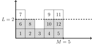
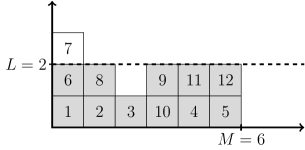
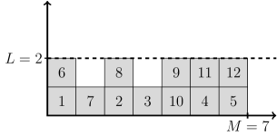
This section is dedicated to the core result of this work: solving Problem in polynomial time. Given a set of jobs with unit processing times and unit resource consumption and a precedence graph with set of arcs , the problem is to find a feasible schedule with makespan at most such that is maximized for a resource level . Figure 2 shows an example of precedence graph with optimal schedules for , and .

For convenience, it will be assumed w.l.o.g. that there are no idling time steps, i.e., time steps where no job is processed, before the makespan of considered schedules. With the above assumption, a schedule can be seen as a sequence of columns, a column being a set of jobs scheduled at the same time step. Note that if two jobs and belong to the same column, there can be no path from to or from to in the precedence graph, in other words, and must be independent.
Problem is closely related to its classical counterpart in makespan minimization: . Among different approaches of the literature to solve in polynomial time, a method relying on maximum matchings between independent jobs is proposed in Fujii et al. [1969]. Since independence between jobs is required for them to be scheduled at the same time step, matching structures naturally appear in a two-machine environment. The results of this section will show that this is still true in the context of resource leveling. Another approach is proposed in Coffman and Graham [1971/1972] with a better time complexity. The idea of this second method is to build a priority list of the jobs based on the precedence graph and then apply the corresponding list-scheduling algorithm. The optimality is proved using a block decomposition of the resulting schedule. In broad outline, the convenient matching structure of the method from Fujii et al. [1969] is used to prove the existence of schedules that satisfy certain objective values while the more efficient method from Coffman and Graham [1971/1972] is used to actually build those schedules.
Two graphs will be considered as support for matchings, both of them being deduced from the precedence graph , as illustrated in Figure 3. First, let be the independence graph where – see Figure 3(a). A critical path in a longest path in the precedence graph. It is a well known result that the sum of processing times along a critical path is the minimum feasible makespan with respect to precedence constraints. Let then be a critical path in . Consider the bipartite graph where , as shown in Figure 3(b) where the jobs of are in gray. Note that in Figure 3, independence relations are represented with dashed lines as opposed to solid lines for precedence relations.

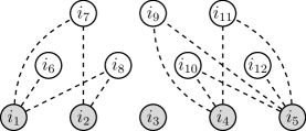
Let and denote the sizes of a maximum matching in and respectively.
The inequality is always verified since is a subset of .
In the example of Figure 3, and .
The aim is to show that the optimal value of objective function can be computed for any using only , , and – and that an associated optimal schedule can be computed in polynomial time.
More precisely, it will be shown that the optimal objective value as a function of , denoted , is piecewise linear with three distinct segments as shown in Figure 4.
Note that if there is no feasible schedule.

The constant part of the function on the right coincides with the result of Fujii et al. [1969] stating that the minimum makespan to schedule the project on two machines is . For , equals its upper bound – all jobs fit under resource level . The contribution of this work is therefore to provide the values of for .
Note that the schedule of Figures 2(b) corresponds to an optimal solution for . Its value is , which is indeed equal to . If the deadline is increased by one, i.e., , then two more jobs can be added under the resource level two, i.e., the optimal value is , as shown in Figure 2(c). It corresponds to the first breaking point in Figure 4, as and . As it can be seen in Figure 2(d), when , all jobs can be scheduled under the resource level. It corresponds to the second breaking point in Figure 4, as .
The proposed approach is in two steps:
-
1.
Find an optimal solution for ;
-
2.
Find recursively an optimal solution for from an optimal solution for .
The following definition introduces the augmenting sequence of a schedule in the independence graphs and in the bipartite independence graph .
Definition 1 (augmenting sequence).
A sequence of distinct jobs is an augmenting sequence for (resp. for ) if:
-
-
is a path in (resp. in );
-
-
the number of jobs scheduled at is not two;
-
-
the number of jobs scheduled at is not two;
-
-
for every , .
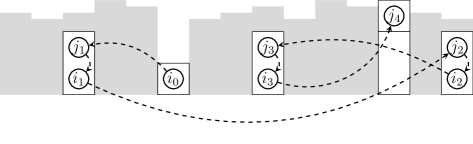
The name augmenting sequence deliberately recalls the augmenting path used in the context of matching problems. It will be seen in the sequel that both notions actually coincide to some extent since an augmenting sequence defines an augmenting path for a certain matching of jobs.
An example of augmenting sequence is illustrated in Figure 5. The jobs of the sequence are surrounded by circles and connected with dashed arrows.
3.1 Solution for
The first step is to solve the problem for the minimum relevant value for , that is to say when equals the length of a critical path in the precedence graph.
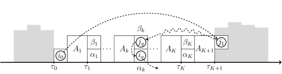
The following definition describes an elementary operation, illustrated in Figure 6, that will be used in the sequel to improve the value of objective function incrementally.
Definition 2 (elementary operation).
Let be a feasible schedule for instance with , where is a critical path of .
Let be two independent jobs such that and such that is the only job scheduled at .
Decomposition: Let us denote the time steps in where at least one predecessor of is scheduled, as well as and for convenience.
For each , the jobs scheduled at are partitioned into and , where are the predecessors of and are the remaining jobs.
Let us also denote, for each , , the sets of jobs scheduled in between the .
Translation: The jobs of are translated from to for each and job from to .


The decomposition and translation steps of Definition 2 are illustrated in Figure 6(a) and Figure 6(b) respectively.
The elementary operation of Definition 2 will now be shown to yield a feasible schedule and its impact on objective function will be quantified.
Proposition 1.
Let be a feasible schedule for instance with , where is a critical path of .
Let be two independent jobs such that and such that is the only job scheduled at .
The schedule resulting from the elementary operation on and is feasible and it verifies:
Proof.
Let us first show that schedule is feasible.
It is clear that the elementary operation does not increase the makespan of the schedule, thus respecting the makespan bound .
By construction, all predecessors of job scheduled between and are in .
As a consequence, there is no precedence arc going from a job of to a job of .
The translation of the elementary operation does no violate any precedence constraint.
Let us now quantify the impact of the elementary operation on the objective function.
Since the makespan bound is , there is exactly one job of critical path at each time step in .
In particular, since is the only job scheduled at , it necessarily belongs to .
Furthermore, for every , a job of is scheduled at .
This job of is a successor of and therefore cannot be in , otherwise and would not be independent, by transitivity.
The job of must then be in , so .
Also, for every by construction.
As a consequence:
-
-
For every , at least two jobs are scheduled at in , which was already the case in
-
-
At least two jobs are scheduled at in while there was only one in
-
-
One less job is scheduled at in
-
-
Other time steps remain unchanged
Job cannot be the only job scheduled at , otherwise would belong to critical path and would not be independent from job . The difference between and comes down to whether there are two or more jobs scheduled at in :
-
-
If exactly two jobs are scheduled at in , then the contribution to the objective function is increased by one in but decreased by one in , so
-
-
If at least three jobs are scheduled at in , then the contribution to the objective function is increased by one in and remains unchanged in , so
∎
Remark 1.
The possibility to improve the objective value of a schedule with makespan using elementary operations will now be linked to the existence of a particular augmenting sequence.
Lemma 1.
Let be a feasible schedule for instance with , where is a critical path of . If there exists an augmenting sequence for such that:
-
-
is the only job scheduled at ;
-
-
at least three jobs are scheduled at ;
then there exists a schedule with makespan such that .
Furthermore, such a schedule can be computed from in polynomial time.
Proof.
The result will be proven using an induction on .
(initialization) For , the augmenting sequence reduces to two jobs and that are independent and scheduled at different dates. The elementary operation can be applied with as and as . Since there are at least three jobs scheduled at , the resulting schedule is such that according to Proposition 1.
(induction) Suppose that the property is verified up to the value for some .
If for some there are at least three jobs scheduled at , then the sequence is an augmenting sequence with the required properties on which the induction hypothesis can be applied.
One can now suppose that for every , the only jobs scheduled at are and .
The idea is now to use the elementary operation of Definition 2 to reduce the size of the augmenting sequence.
Assume that the elementary operation is applied using as and as and let be the resulting schedule.
If is an augmenting sequence for , then the induction can be applied.
If not, there exists such that coincide with in the decomposition of Definition 2, implying that .
In that case, schedule would be irrelevant for the induction.
Such a crossing configuration is illustrated in Figure 7(a).
Moreover, let us show that and .
Since the augmenting sequence is a path in the bipartite graph , it alternates between jobs of the critical path and jobs of .
In a schedule of makespan , exactly one job belongs to at each time step, so that is the only job scheduled at belongs to and so do .
By construction, in the decomposition of Definition 2, only block can contain successors of .
Therefore, that is a successor of since it is in the critical path must be in .
The only other job scheduled at is and it must belong to that cannot be empty.
Having guarantees that is independent from , so is an edge in .
A shortcut can then be operated from to , as illustrated in Figure 7(b), yielding sequence that is an augmenting sequence on which the induction hypothesis applies.

∎
Proposition 2.
Any optimal solution of the instance with verifies . Furthermore, such an optimal schedule can be computed in polynomial time.
Proof.
Let us first show that the objective function value for a feasible schedule is at most .
Let be a feasible schedule with makespan .
Let be the number of time steps in with at least two jobs scheduled in .
It is clear that .
By definition of a critical path, exactly one job of is scheduled at every time step of .
Given that two jobs scheduled at the same time step are necessarily independent, matching each job of the critical path with a job that is scheduled at the same date, when there is one, yields a matching in .
In other words, a matching of size in can be deduced from , so and .
It will now be shown that there exists a feasible schedule such that .
Suppose that a given schedule is such that there are time steps in where at least two jobs are scheduled, with .
Again, and it is possible to deduce from a matching of size in .
This matching being not of maximum size, Berge’s theorem [Berge, 1957] states that there exists an augmenting path.
Let denote the sequence of jobs in the augmenting path, with , and both being not matched in .
The following properties hold:
-
-
is a job of that is not matched in , so it is the only one scheduled at .
-
-
is a job of that is not matched in . Since there is a job of at each time step, is scheduled at together with a job of . This job of could be matched with in but it is not so, by construction of , it must be matched with a third job. Thus, three jobs are scheduled at .
-
-
and are matched together in so for every .
Those properties imply that is an augmenting sequence satisfying the requirements of Lemma 1. Applying Lemma 1 gives that there exists a schedule with . As a conclusion, any feasible schedule of can be modified incrementally to reach an objective function value of . ∎
3.2 Solution for
The problem will now be solved for other values of based on the solution for . The idea is to apply transformations that increment the makespan of the initial schedule while keeping its optimality. First, it will be shown that optimal solutions always reach makespan deadline when is in a certain interval.
Lemma 2.
For any makespan deadline any optimal schedule for has makespan exactly .
Proof.
Let and suppose that there exists an optimal schedule for of makespan .
According to the result of Fujii et al. [1969], the minimum makespan to schedule the project on two machines is .
This implies that there exists a time step where at least three jobs are scheduled in .
Consider the transformation illustrated in Figure 8.
One of the jobs scheduled at can be scheduled at instead and the subsequent jobs can be scheduled one time step later.
The resulting schedule has makespan and objective value .
This contradicts the optimality of since is feasible for with a strictly higher objective value.
∎

Lemma 3.
Let and let be an optimal schedule for .
Suppose that is such that, at each time step , either , or jobs are scheduled.
If there exists an augmenting sequence for satisfying ,
then there exists a schedule with makespan such that .
Furthermore, such a schedule can be computed from in polynomial time.
Proof.
Some useful properties of the augmenting sequence are first derived from basic transformations.
An augmenting sequence can indeed be obtained in which and are the only jobs scheduled at for every .
Suppose that three jobs are scheduled at for some , two cases are possible:
-
-
if is scheduled at , then the sequence is an augmenting sequence and satisfies ;
-
-
otherwise the sequence is an augmenting sequence satisfying .
In both cases, an augmenting sequence with the required properties can be obtained by truncating the initial one. Such truncations can be operated on the augmenting sequence until all intermediary time steps have exactly two jobs scheduled.
It can also be ensured that no arc of the augmenting sequence jumps over a time step different from and with exactly three jobs scheduled. Indeed, suppose that an arc of the augmenting sequence is such that there exists a job with exactly three jobs scheduled at and w.l.o.g. , as shown in Figure 9. Since and are independent, is either independent from or from – or both. If is independent from , then the augmenting sequence can be truncated after and ended with arc . If is independent from , then the augmenting sequence can be truncated before and started with arc .
One can now suppose that the augmenting sequence is such that:
-
-
and are the only jobs scheduled at for every ;
-
-
for every arc and every time step , at most two jobs are scheduled at .
Let and .
For every time step , either or jobs are scheduled at .
Consider the subset of jobs .
Let denote the matching on obtained by pairing the jobs scheduled at the same time step.
It is clear that is a matching between independent jobs of of size .
Using the result of Fujii et al. [1969], it is possible to schedule the jobs of on two machines using at most time steps.
Three cases can be distinguished, only one of which is actually possible:
- 1.
-
2.
If either or is scheduled alone on its time step – the other being on a time step with exactly three jobs, the jobs of are scheduled on time steps in . This contradicts the optimality of since, using Fujii et al. [1969], all jobs of can be scheduled on the same number of time steps without exceeding the resource level.
-
3.
If both and are scheduled on time steps with exactly three jobs, the jobs of are scheduled on time steps in . Using Fujii et al. [1969], these jobs can be scheduled on time steps without exceeding the resource level, so the objective function can be increased by . This is the expected result.
∎
Lemma 4.
For any , , the optimal objective function verifies:
Proof.
Using Proposition 2 and by definition of , in any feasible schedule, at most jobs of are scheduled on the same time step as a job of .
Equivalently, at least jobs of are alone on their time step in any feasible schedule.
This implies that for any , , which can be rewritten as .
∎
Lemma 5.
For any , , the optimal objective function verifies:
Proof.
Let , , and suppose that there exists a feasible schedule for such that . At least time steps have two or more jobs scheduled in . A matching between independent jobs of size at least can then be deduced from . By definition of as the maximum size for a matching between independent jobs, and . Inequality is then verified for any feasible schedule so . ∎
The following theorem allows for the computation of as a function of as illustrated in Figure 4.
Theorem 1.
The optimal objective function value as a function of makespan deadline is piecewise linear and defined as follows:
-
-
For : ;
-
-
For : ;
-
-
For , : .
Furthermore, an optimal schedule can be computed for any in polynomial time.
Proof.
Let us prove by induction on that there exists a schedule of makespan such that for every .
The case of was solved in Section 3.1.
Suppose that the property holds for some and let be the associated schedule.
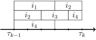
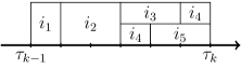
If there exists a time step with at least jobs scheduled in , two of those jobs can be scheduled on the next time step while all jobs scheduled after are postponed by one time unit, as illustrated in Figure 10.
This yields an optimal schedule .

If not, satisfies the requirement of Lemma 3 since either , or jobs are scheduled at each time step . Let denote a matching obtained by selecting a pair of jobs for each time step where at least two jobs are scheduled in . Since according to the induction hypothesis, there are such time steps. It is then clear that is a matching between independent jobs of size . This matching is not maximum because . By Berge’s Theorem, there exists an augmenting path in such that for each and such that neither nor are matched in . Notice the following:
-
-
If exactly two jobs were scheduled at , would be in . Either or jobs are scheduled at .
-
-
If exactly two jobs were scheduled at , would be in . Either or jobs are scheduled at .
-
-
By construction of , for every .
Furthermore, if and were equal, three jobs would be scheduled at and at least one job in would be matched in . As a consequence, . All the requirements of Lemma 3 are now satisfied by and . Applying Lemma 3 gives that there exists a schedule of makespan such that . This value reaches the upper bound of Lemma 4 so is optimal.
Let us prove by induction on that there exists a schedule of makespan such that for every .
The case of follows from the previous case.
Suppose that the property holds for some and let be the associated schedule.
Using the induction hypothesis, and, since , .
There must exist a time step with at least three jobs scheduled in .
A schedule with makespan and such that can be obtained using one-job elongation as shown in Figure 8.
This value reaches the upper bound of Lemma 5 so is optimal.
For , the schedule obtained through the method of Fujii et al. is always optimal since it reaches the natural upper bound of the objective function. ∎
3.3 Algorithm
The main steps in the resolution of are summarized in Algorithm 1. Schedule computation steps are not detailed but rely in particular on the proofs of Lemma 1 and Lemma 3.
Let us discuss the time complexity of Algorithm 1. An important point to note is that, although the method of Fujii et al. [1969] has been used, due to its convenient matching structure, to prove that is polynomial, it is not the most computationally efficient. Therefore, solving problem when applying Lemma 3 is done using the more efficient method of Coffman and Graham [1971/1972]. The time required to perform the different computation steps is as follows:
-
-
Computing the transitive closure of precedence graph :
-
-
Solving the problem for :
-
-
Finding an augmenting sequence (alternating path in bipartite independence graph ):
-
-
Elementary operation:
-
-
Size of an augmenting path:
-
-
Maximum number of augmenting sequences to find:
Total to solve the case:
-
-
- -
Total computation time of Algorithm 1 is therefore .
4 Further tractable special cases
In this section, five resource leveling problems are shown to be solvable in polynomial or pseudo-polynomial time. Section 5 will show that further generalization of those special cases leads to strongly -hard problems.
Precedence constraints, as considered in the core problem of this work, are classical scheduling constraints and are present in many practical applications. However, is very specific and solving problems with other values of can be interesting. Section 4.1 shows that, when precedence graphs are restricted to in-trees, the problem is solved to optimality for any by adapting Hu’s algorithm [Hu, 1961]. Unit processing times is also a strong assumption and results for more general values can be of use. Section 4.2 shows that restricting the resource level to yields another polynomial special case for any processing times.
Release and due dates are other classical scheduling constraints that can be studied together with a resource leveling objective. Polynomial solving methods are given for two problems with release dates and due dates in which preemption is allowed. Section 4.3 deals with by translating it as a flow problem. Section 4.4 solves using linear programming.
Finally, Section 4.5 shows that, when there are no precedence constraints, a tractable method exists for non-unit processing times and resource consumptions. A pseudo-polynomial algorithm is provided for based on dynamic programming.
4.1 A polynomial algorithm for
The classical scheduling problem can be solved in polynomial time using Hu’s algorithm [Hu, 1961].
In this section, its leveling counterpart is considered, namely .
The idea is therefore to adapt the algorithm proposed in Hu [1961] in order to obtain a polynomial algorithm to solve .
Hu’s algorithm can be applied in the case of Unit Execution Times (UET) when the precedence graph is an in-tree.
It is a list algorithm in which jobs are sorted in increasing order of latest starting time.
The following algorithm uses the same priority list: jobs with small latest starting time are scheduled first.
However, since the jobs are constrained by the deadline , the algorithm must execute at a given time the jobs whose latest starting time is and that have not been scheduled yet.
This can cause the resource level to be exceeded.
In order for a feasible schedule to exist, the deadline chosen as input for UETInTreeLeveling should be at least the length of the critical path in the precedence graph – which is the depth of the in-tree in the present case.
Furthermore, it can be assumed that , which ensures that UETInTreeLeveling is executed in polynomial time.
UETInTreeLeveling returns schedules with a very specific structure.
The following lemma gives some of those specificities that will prove to be useful in showing that UETInTreeLeveling is actually optimal.
Lemma 6.
Let be the schedule returned by UETInTreeLeveling.
Suppose that at a given time step the set of jobs scheduled at in is such that .
The following assertions are true:
-
(i) Every has latest starting time ;
-
(ii) For every , ;
-
(iii) For every , every has latest starting time .
Proof.
First, it is clear that when time step is reached in UETInTreeLeveling, all jobs with latest starting time at most have already been scheduled.
This is true thanks to the instruction of line 5 that ensures that all jobs reaching their latest starting time are scheduled.
As a consequence, all jobs with latest starting time that remain in are leaves and they have the lowest value.
There are at least such jobs otherwise it would be impossible to have .
The instruction of line 4 therefore selects jobs with latest starting time and instruction of line 5 adds the remaining ones to .
This proves assertion (i).
Due to assertion (i) and since , there are at least jobs with latest starting time .
For any , is a subtree of so has at least leaves corresponding to jobs with latest starting time at most .
In particular, has at least leaves, which ensures that and proves assertion (ii).
Since UETInTreeLeveling prioritizes jobs with lower values and since for any , has at least leaves corresponding to jobs with latest starting time or less, no job with latest starting time strictly higher than can be scheduled at or before.
This proves assertion (iii).
∎
Proposition 3.
is solvable in polynomial time using UETInTreeLeveling.
Proof.
Let be the schedule returned by UETInTreeLeveling.
Figure 11 gives an example of such a schedule and illustrates the decomposition of the objective function that follows.
For any time step , let denote the set of jobs scheduled at in .
First, is a feasible schedule.
Indeed, by selecting leaves of the subtree , the instruction of line 4 ensures that the predecessors of the selected jobs have already been scheduled, thus satisfying precedence constraints.
As for the deadline constraint, it is satisfied thanks to the instruction of line 5 that ensures that each job is scheduled no later than its latest starting time.
If for every , , then is optimal since , which reaches a natural upper bound on .
If not, let be the largest time step such that .
In any feasible schedule, all jobs with latest starting time must be scheduled at or before.
It implies that only jobs with latest starting time can be scheduled on time steps .
An upper bound on is therefore given by .
Assertion (ii) of Lemma 6 gives that the contribution to of interval is .
Since is the last time step such that and given assertion (iii) of Lemma 6, all jobs of are scheduled on time steps without exceeding resource level .
It then holds that the contribution to of interval is .
Finally, the value of writes:
which reaches the previously given upper bound and is therefore optimal. ∎
4.2 A polynomial algorithm for
Suppose that and that for every .
Let us also assume that the makespan deadline is larger than the longest path in the precedence graph – otherwise no feasible schedule exists.
For any , let us denote the latest starting time of job , i.e., the makespan deadline minus the longest path from job in the precedence graph .
Algorithm UnitResourceLeveling below starts by scheduling jobs sequentially in a topological order and then schedules the remaining ones at their latest starting time.
Proposition 4.
UnitResourceLeveling solves in polynomial time.
Proof.
Let us prove that UnitResourceLeveling can be executed in time (recall that is the set of arcs in the precedence graph).
First, values for every as well as the topological order can be computed with a graph traversal in time.
As for the main loop, it can be executed in time.
Let us now prove that UnitResourceLeveling provides a schedule that maximizes the time during which at least one unit of resource is used.
In the particular case where , it is easily seen that all the jobs can be scheduled consecutively in a topological order thus leading to a resource usage that is always at most .
It is exactly what the algorithm does since, when , the inequality always holds on line 5.
If then there exists such that .
Let be the first such index.
In the schedule returned by UnitResourceLeveling, jobs are scheduled consecutively without interruption on time interval .
By definition of , the jobs on a longest path starting from are executed without interruption on time interval .
Given that , the returned schedule uses at least one unit of resource constantly on time interval .
The amount of resource below the level is therefore maximized.
Also note that the vector returned by UnitResourceLeveling is a feasible schedule as it satisfies precedence constraints.
Indeed, given an arc of the precedence graph it is clear that, by definition, and that comes before in any topological order.
If , then and therefore .
Assuming that and in the topological order, if , then and therefore .
∎
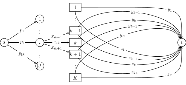
4.3 A polynomial algorithm for
The aim of this section is to show that Problem reduces to a linear program. Let be such that . For convenience, let also . The following variables are considered:
-
-
: the number of time units of job processed during interval ;
-
-
: number of time units processed on interval not exceeding the resource level;
-
-
: number of time units processed on interval over the resource level;
Note that the following program only provides an implicit solution of Problem .
Variables give the number of time units of a job in the interval but this does not tell when each individual time unit is executed.
It will be shown later that an algorithm can be used to deduce a fully-fledged solution of from values.
The program writes:
| (1) | |||||
| (2) | |||||
| (3) | |||||
| (4) | |||||
| (5) | |||||
Note that in this program, maximizing is equivalent to minimizing since . The alternative program writes:
It can be interpreted as a minimum cost flow problem. Figure 12 shows the structure of the flow graph with flow values on arcs. The costs are equal to one for arcs with and otherwise. Arcs with have capacity , arcs with have capacity and arcs with have infinite capacity.
An explicit solution of Problem can be constructed with an additional post-processing step.
Consider the interval for some in and let .
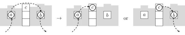
The following algorithm, illustrated in Figure 13, computes the sub-intervals of on which each job of is executed.
Its idea is simple: the interval is filled line by line from left to right by placing one job after another and starting a new line every time the end of the interval is reached.
Those line breaks may cause a job to be split into two parts, one reaching the end of the interval and the other starting back from the beginning.
It is clear that IntervalScheduling is executed in time. Executing it for each can therefore be done in . Note that in the solution provided by IntervalScheduling, each job is executed on either one or two sub-intervals of . As a consequence, each job is executed on at most disjoint intervals in the final solution.
Proposition 5.
is solvable in polynomial time.
Proposition 6.
is solvable in polynomial time.
Proof.
Since reduces to a minimum cost flow problem, standard algorithms can be used to solve it and yield integer solutions when . In particular, optimal integer solutions can be found for , which is actually the same as finding optimal solutions for . ∎
4.4 A polynomial algorithm for
Similarly as in Section 4.3, the aim of this section is to show that problem reduces to a linear program.
It will be assumed that all considered instances are feasible, namely that for every job .
In Problem , the resource consumption of job can take any value in , yet it is sufficient to consider the case where .
Indeed, since objective function only takes into consideration the resource consumption that fits under resource level , any can be handled as without changing the optimum.
As for potential jobs , they have no impact on the objective.
Let us then suppose that for every and denote and . Let be such that . For convenience, let also . The following variables are considered:
-
-
: the number of time units of job processed during interval that fit under the resource level;
-
-
: the number of time units of job processed during interval that fit under the resource level.
Just like in Section 4.3, the following linear program only gives an implicit solution of the problem from which a proper schedule can then be deduced. The program writes:
| (6) | |||||
| (7) | |||||
| (8) | |||||
| (9) | |||||
| (10) | |||||
A complete solution in which each job is given a set of intervals on which it is executed can be deduced from optimal values of and variables. Recall that variable and only represent the portions of the jobs that fit under the resource level. Those portions of jobs are scheduled on each interval as shown in Figure 14: the jobs of are scheduled first, then the jobs of are scheduled in the remaining space with Algorithm 4. Once this is done, the processing time left for each job can be scheduled anywhere in the remaining space of its availability interval . The initial assumption that for every job ensures that it is possible to do so.
Proposition 7.
is solvable in polynomial time.
Remark 2.
Unlike in the case of Section 4.3, nothing guarantees to find integer solution to the problem.
Remark 3.
The method can be generalized to Problem , in which jobs either consume one or units of resource.
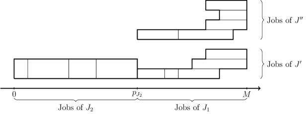
4.5 A pseudo-polynomial algorithm for
In order to solve in pseudo-polynomial time, some assumptions are made w.l.o.g. to exclude trivial cases. First, it can be assumed that resource consumptions values are in . Indeed, when , replacing resource consumption of each job by does not change the objective function values. Jobs with resource consumption have no impact and can be scheduled at any feasible date, they can be ignored. Only jobs with are to be considered in the sequel.
Let us denote and . Let also and . If , the problem is solved simply by scheduling the jobs of one after another while possible and at their latest possible date afterwards. This uses at least two units of resource constantly on thus maximizing . Let us therefore assume that .
The following lemma links the objective value of a schedule to a subset of , allowing for the construction of the former from the latter.
Lemma 7.
Let be an instance of .
For any subset of jobs , there exists a schedule such that:
Furthermore, can be computed in polynomial time.
Proof.
The schedule is built as follows and as illustrated in Figure 15:
-
-
The jobs of are scheduled one after the other from to .
-
-
The jobs of are scheduled one after the other, starting from , while the makespan deadline is not exceeded and at their latest possible date afterwards.
-
-
The jobs of are scheduled as the jobs of
The schedule is such that:
-
-
The jobs of use exactly two units of resource on ;
-
-
The jobs of use at least one unit of resource on ;
-
-
The jobs of use at least one unit of resource on .
This implies that . ∎
Having two jobs of that overlap in a schedule is never advantageous in terms of leveling objective. This idea is formalized in the following lemma:
Lemma 8.
The schedules in which the jobs of do not overlap are dominant.
Proof.
One job of is sufficient to reach resource level for its whole duration and overlapping with another job is a missed contribution to function . Given the previous assumption that , it is always possible to find an optimal schedule in which the jobs of do not overlap. ∎
The following lemma complements the inequality of Lemma 7 by another inequality that is valid when the jobs of do not overlap.
Lemma 9.
Let be an instance of and let be a feasible schedule for such that the jobs of do not overlap.
Then there exists a subset of jobs such that:
Proof.
Let us build two disjoint subsets from using the following procedure:
Let us denote (resp. ) the set of time steps where no job of is processed and where at least one job of (resp. ) is processed. It is clear that and . For any time step , three cases are possible:
-
-
: at least two jobs of are processed at time step in , one being in and another in ;
-
-
: exactly one job of is processed at time step in , it is either in or in ;
-
-
: either a job of is processed at time step in or no job at all, otherwise it would have been added to either or in the procedure.
In other words, and as a consequence . The final inequality is derived using that . ∎
Thanks to Lemma 8, the inequality of Lemma 9 actually applies to any schedule. Combining it with the inequality of Lemma 7 yields the following equality:
| (11) |
It is then clear that if a subset is found that maximizes , the maximum value of over feasible schedules can be deduced directly. Furthermore, using Lemma 7, it is actually possible to build a schedule from such that:
Schedule thus maximizes , it is an optimal solution of the problem.
A possible interpretation of Equation 11 is that solving is equivalent to solving a two-machine early work maximization problem on the jobs of : subset (resp. ) corresponds to the jobs scheduled on the first (resp. second) machine and the portion of jobs executed before date is maximized. By complementarity of the early and late work criterions, the equivalence with the late work minimization version of the problem also holds. Late work minimization on two machines with common deadline, namely is studied in Chen et al. [2016] and shown to be solvable in pseudo-polynomial time. Applying the algorithm proposed in Chen et al. [2016] leads to a solution method for running in . Yet, finding an optimal subset can be done with a better time complexity using standard dynamic programming. A table can be computed in time where if there exists a subset of the first jobs of whose sum is and otherwise. Then, for each such that , the values of can be computed in order to find the maximum value. This maximum value is optimal and the corresponding optimal subset can be recovered with a standard backward technique in time .
This leads to the following proposition:
Proposition 8.
Problem can be solved in time.
Proof.
A subset that maximizes can be built in time using dynamic programming.
Lemmas 7 and 9 guarantee that satisfies .
Moreover, lemma 7 states that a schedule can be built from that maximizes .
This can be done in time.
An optimal schedule for an instance of problem can therefore be found with a total computation time of .
∎
5 -hardness results
Some of the algorithms presented in the previous sections highlight similarities between resource leveling and classical scheduling problems in terms of solution. This section shows that hardness results easily transfer from machine scheduling problems to their leveling counterparts. This will follow from the Lemma 10; it intuitively shows that resource leveling problems can be seen as generalizations of classical machine scheduling problems.
Lemma 10.
Let be an instance of for some and some set of constraints .
Let be an instance of .
The two following assertions are equivalent:
-
(i) has a solution of makespan at most
-
(ii) has a feasible schedule with
Proof.
First note that a solution of is described by a schedule and a partition of such that is the subset of non-overlapping jobs processed on the -th machine.
(i) (ii) Let then be a feasible solution of with makespan at most .
It is clear that the schedule is a feasible schedule for since it satisfies the constraints of and has makespan at most .
Furthermore, the jobs can be processed on machines, which implies that the resource consumption never exceeds and gives that .
As a consequence, has a feasible schedule with .
(i) (ii) Let be a feasible schedule for such that .
Using the following procedure, let us build a partition of such that each is a subset of non-overlapping jobs.
The claim is that when is selected on line 5, . Indeed, if , by definition of , all machines are loaded and at least jobs are being processed simultaneously on the non-empty interval , implying that , which is a contradiction. The inequality being verified at each step of the procedure guarantees that the jobs in each do not overlap. A feasible solution for with makespan at most is therefore given by . ∎
The equivalence of Lemma 10 provides a general reduction from a problem of the form to a problem of the form . The -hardness (resp. strong -hardness) of the former thus implies the -hardness of the latter.
Corollary 1.
The problems listed below are strongly -hard:
-
-
-
-
-
-
-
-
Problem is -hard.
Proof.
Remark 4.
While and are known to be strongly -hard, which can be used to prove the complexity of their leveling counterparts, the complexity of remains unknown. It is then not possible to get a complexity result for based on Lemma 10.
The -hardness of can actually be extended to the case of quite naturally: an instance of reduces to an instance of with an additional job verifying , and since job uses one unit of resource from to . Hence the following corollary:
Corollary 2.
is strongly -hard.
Another easy extension of Corollary 1 can be made to prove that is strongly -hard. It requires to notice that an instance of reduces to an instance of where each job in is given a predecessor and a successor that force it to be scheduled in its availability interval. More precisely, for a job in , two jobs and are added with , , and precedence constraints and . This gives the following corollary:
Corollary 3.
is strongly -hard.
6 Summary of results
Table 1 summarizes the complexity results that were obtained in this work.
Column headers are classical scheduling constraints: makespan deadline (), precedence constraints (), possibly in the form of an and release and due dates (), which may be considered with or without preemption ().
Row headers are parameters restrictions: the value of may be restricted to one or two while unit values may be imposed for processing times and resource consumptions.
The entries of the table include the complexity of the corresponding problem as well as the result proving it.
A natural question arising from this table is the complexity of problems for or larger constant , in particular .
This latter problem generalizes , the complexity of which is a famous open problem in scheduling.
Remark 5.
Problem is solved to optimality by scheduling jobs with one after another while is not exceeded and scheduling all remaining jobs at .
In the case of Problem , all jobs are independent from each other and equivalent, with unit processing time and resource consumption.
It is clear that scheduling one job per time step sequentially, going back to when is reached, solves the problem to optimality.
| in (Remark 5) | str. -hard (Cor. 3) | str. -hard (Cor. 1) | in (Prop. 5) | |||
| in (Prop. 4) | ||||||
| in (Prop. 8) -hard (Cor. 1) | str. -hard (Cor. 1) | str. -hard (Cor. 2) | in (Prop. 7) | |||
| in (Remark 5) | in (Th. 1) | in (Prop. 6) | ||||
| str. -hard (Cor. 1) | str. -hard [Györgyi and Kis, 2020] | |||||
| in (Prop. 5) | ||||||
| in (Remark 5) | str. -hard (Cor. 1) , | in (Prop. 3) | in (Prop. 6) | |||
7 Conclusion
A polynomial-time algorithm solving a resource leveling counterpart of a well-known two-processor scheduling problem is proposed in this paper as a main result. As complementary results, various related resource leveling problems are studied, some of which are shown to be solvable in polynomial time as well. Close links are highlighted between classical machine scheduling resource leveling. Both solving methods and -hardness results are mirrored from one field to the other. While the translation of negative complexity results is rather straightforward, the main contribution of this work lies on the design of algorithms. Besides the core problem, an interesting result in that regard is the adaptation of Hu’s algorithm to solve the case of unit processing times with unit resource consumptions and an in-tree precedence graph.
Although polynomial and pseudo-polynomial algorithms are given, the problem variants that they can solve remain special cases.
An interesting perspective would be to consider more advanced constraints and less restrictive parameters, to meet practical requirements.
In particular, some problem variants are polynomial for unit processing times but become strongly -hard in the general case.
A possible extension of this work would then be to find good approximation algorithms for some of the more realistic resource leveling problems.
The objective function that was chosen is certainly relevant to model resource overload costs, yet it does not prevent peaks in resource use, which are often ill-advised in practice.
Studying the resource investment objective, which minimizes the highest amount of resource consumption, could therefore be another perspective for future research.
| General | |
| Set of jobs | |
| Processing time of job | |
| Resource consumption of job | |
| Precedence graph | |
| Set of arcs in | |
| Schedule | |
| Starting time of job in schedule | |
| Resource level | |
| Deadline on makespan | |
| Objective function | |
| Critical path in | |
| Scheduling constraints | |
| Makespan | |
| Precedence constraints | |
| In-tree precedence graph | |
| Preemption allowed | |
| Release date of job | |
| Due date of job | |
| Auxiliary graphs | |
| Independence graph | |
| Set of edges in | |
| Size of a maximum matching in | |
| Bipartite independence graph for critical path | |
| Set of edges in | |
| Size of a maximum matching in | |
References
- Atan and Eren [2018] T. Atan and E. Eren. Optimal project duration for resource leveling. European Journal of Operational Research, 266(2):508–520, 2018.
- Berge [1957] C. Berge. Two theorems in graph theory. Proceedings of the National Academy of Sciences, 43(9):842–844, 1957.
- Bianco et al. [2016] L. Bianco, M. Caramia, and S. Giordani. Resource levelling in project scheduling with generalized precedence relationships and variable execution intensities. OR spectrum, 38(2):405–425, 2016.
- Bianco et al. [2017] L. Bianco, M. Caramia, and S. Giordani. The total adjustment cost problem with variable activity durations and intensities. European Journal of Industrial Engineering, 11(6):708–724, 2017.
- Chen et al. [2016] X. Chen, M. Sterna, X. Han, and J. Blazewicz. Scheduling on parallel identical machines with late work criterion: Offline and online cases. Journal of Scheduling, 19:729–736, 2016.
- Chen et al. [2020] X. Chen, Y. Liang, M. Sterna, W. Wang, and J. Błażewicz. Fully polynomial time approximation scheme to maximize early work on parallel machines with common due date. European Journal of Operational Research, 284(1):67–74, 2020.
- Christodoulou et al. [2015] S. E. Christodoulou, A. Michaelidou-Kamenou, and G. Ellinas. Heuristic methods for resource leveling problems. In Handbook on Project Management and Scheduling Vol. 1, pages 389–407. Springer, 2015.
- Coffman and Graham [1971/1972] E. Coffman, Jr. and R. Graham. Optimal scheduling for two-processor systems. Acta Informat., 1:200–213, 1971/1972.
- Demeulemeester [1995] E. Demeulemeester. Minimizing resource availability costs in time-limited project networks. Management Science, 41(10):1590–1598, 1995.
- Drótos and Kis [2011] M. Drótos and T. Kis. Resource leveling in a machine environment. European Journal of Operational Research, 212(1):12–21, 2011.
- Du et al. [1991] J. Du, J.-T. Leung, and G. Young. Scheduling chain-structured tasks to minimize makespan and mean flow time. Inform. and Comput., 92(2):219–236, 1991.
- Easa [1989] S. M. Easa. Resource leveling in construction by optimization. Journal of construction engineering and management, 115(2):302–316, 1989.
- Fujii et al. [1969] M. Fujii, T. Kasami, and K. Ninomiya. Optimal sequencing of two equivalent processors. SIAM Journal on Applied Mathematics, 17(4):784–789, 1969.
- Garey and Johnson [1978] M. Garey and D. Johnson. Strong NP-completeness results: motivation, examples, and implications. J. Assoc. Comput. Mach., 25(3):499–508, 1978.
- Garey and Johnson [1977] M. R. Garey and D. S. Johnson. Two-processor scheduling with start-times and deadlines. SIAM journal on Computing, 6(3):416–426, 1977.
- Graham et al. [1979] R. L. Graham, E. L. Lawler, J. K. Lenstra, and A. R. Kan. Optimization and approximation in deterministic sequencing and scheduling: a survey. In Annals of discrete mathematics, volume 5, pages 287–326. Elsevier, 1979.
- Györgyi and Kis [2020] P. Györgyi and T. Kis. A common approximation framework for early work, late work, and resource leveling problems. European Journal of Operational Research, 286(1):129–137, 2020.
- Hartmann and Briskorn [2022] S. Hartmann and D. Briskorn. An updated survey of variants and extensions of the resource-constrained project scheduling problem. European Journal of operational research, 297(1):1–14, 2022.
- Hu [1961] T. C. Hu. Parallel sequencing and assembly line problems. Operations research, 9(6):841–848, 1961.
- Lenstra et al. [1977] J. Lenstra, A. Rinnooy Kan, and P. Brucker. Complexity of machine scheduling problems. Ann. of Discrete Math., 1:343–362, 1977.
- Li and Dong [2018] H. Li and X. Dong. Multi-mode resource leveling in projects with mode-dependent generalized precedence relations. Expert Systems with Applications, 97:193–204, 2018.
- Li et al. [2018] H. Li, L. Xiong, Y. Liu, and H. Li. An effective genetic algorithm for the resource levelling problem with generalised precedence relations. International Journal of Production Research, 56(5):2054–2075, 2018.
- Micali and Vazirani [1980] S. Micali and V. V. Vazirani. An algorithm for finding maximum matching in general graphs. In 21st Annual Symposium on Foundations of Computer Science (FOCS 1980), pages 17–27. IEEE, 1980.
- Neumann and Zimmermann [1999] K. Neumann and J. Zimmermann. Resource levelling for projects with schedule-dependent time windows. European Journal of Operational Research, 117(3):591–605, 1999.
- Ponz-Tienda et al. [2017a] J. L. Ponz-Tienda, A. Salcedo-Bernal, and E. Pellicer. A parallel branch and bound algorithm for the resource leveling problem with minimal lags. Computer-Aided Civil and Infrastructure Engineering, 32(6):474–498, 2017a.
- Ponz-Tienda et al. [2017b] J. L. Ponz-Tienda, A. Salcedo-Bernal, E. Pellicer, and J. Benlloch-Marco. Improved adaptive harmony search algorithm for the resource leveling problem with minimal lags. Automation in Construction, 77:82–92, 2017b.
- Qiao and Li [2018] J. Qiao and Y. Li. Resource leveling using normalized entropy and relative entropy. Automation in Construction, 87:263–272, 2018.
- Rieck and Zimmermann [2015] J. Rieck and J. Zimmermann. Exact methods for resource leveling problems. In Handbook on Project Management and Scheduling Vol. 1, pages 361–387. Springer, 2015.
- Rieck et al. [2012] J. Rieck, J. Zimmermann, and T. Gather. Mixed-integer linear programming for resource leveling problems. European Journal of Operational Research, 221(1):27–37, 2012.
- Rodrigues and Yamashita [2015] S. B. Rodrigues and D. S. Yamashita. Exact methods for the resource availability cost problem. In Handbook on Project Management and Scheduling Vol. 1, pages 319–338. Springer, 2015.
- Sterna [2011] M. Sterna. A survey of scheduling problems with late work criteria. Omega, 39(2):120–129, 2011.
- Sterna and Czerniachowska [2017] M. Sterna and K. Czerniachowska. Polynomial time approximation scheme for two parallel machines scheduling with a common due date to maximize early work. Journal of Optimization Theory and Applications, 174:927–944, 2017.
- Ullman [1975] J. Ullman. NP-complete scheduling problems. J. Comput. System Sci., 10:384–393, 1975.
- Van Peteghem and Vanhoucke [2013] V. Van Peteghem and M. Vanhoucke. An artificial immune system algorithm for the resource availability cost problem. Flexible services and manufacturing journal, 25(1):122–144, 2013.
- Verbeeck et al. [2017] C. Verbeeck, V. Van Peteghem, M. Vanhoucke, P. Vansteenwegen, and E.-H. Aghezzaf. A metaheuristic solution approach for the time-constrained project scheduling problem. OR spectrum, 39(2):353–371, 2017.
- Woodworth and Willie [1975] B. M. Woodworth and C. J. Willie. A heuristic algorithm for resource leveling in multi-project, multi-resource scheduling. Decision Sciences, 6(3):525–540, 1975.
- Zhu et al. [2017] X. Zhu, R. Ruiz, S. Li, and X. Li. An effective heuristic for project scheduling with resource availability cost. European journal of operational research, 257(3):746–762, 2017.