Learnable & Interpretable Model Combination
in Dynamic Systems Modeling

Abstract

One of the core concepts in science, and something that happens intuitively in every-day dynamic systems modeling, is the combination of models or methods. Especially in dynamical systems modeling, often two or more structures are combined to obtain a more powerful or efficient architecture regarding a specific application (area). Further, even physical simulations are combined with machine learning architectures, to increase prediction accuracy or optimize the computational performance. In this work, we shortly discuss, which types of models are usually combined and propose a model interface that is capable of expressing a width variety of mixed algebraic, discrete and differential equation based models. Further, we examine different established, as well as new ways of combining these models from a system theoretical point of view and highlight two challenges - algebraic loops and local event affect functions in discontinuous models - that require a special approach. Finally, we propose a new wildcard topology, that is capable of describing the generic connection between two combined models in an easy to interpret fashion that can be learned as part of a gradient based optimization procedure. The contributions of this paper are highlighted at a proof of concept: Different connection topologies between two models are learned, interpreted and compared applying the proposed methodology and software implementation.

1 Introduction

With the goal to further optimize regression and classification models of dynamical systems, one of the current trends in machine learning is the combination of existing models such that their positive characteristics are merged. This comes in different flavors: For example, in [1] recurrent, convolutional and linear continuous-time differential equations are combined to improve speech classification. Or [2] introduces the combination of a (neural) ordinary differential equation (ODE), a recurrent neural network (RNN) and an additional feed-forward neural network (FFNN), called ODE-RNN, that improves the capability of pure RNN of handling irregular sampled data. In the domain of scientific machine learning, machine learning structures are paired with powerful algorithms from scientific computing (like differential equation solvers). This is for example the case for neural ODEs, so neural networks that are solved by numerical integration, as introduced in [3]. In hybrid modeling, existing simulation models can be extended by an additional machine learning part (or the other way round), often to learn for unknown (or not modeled) physical effects, as for example the arterial cross-section change by pressure in the human cardiovascular system as in [4].

The meaning of the term model differs between the mentioned application domains: Deep FFNNs for example, describe a nonlinear mapping from the input of the first layer $\bm{u}$ to the output of the last layer $\bm{y}$. RNNs on the other hand, additionally depend on the internal hidden state of the architecture. Common simulation models of dynamical systems (like from physics or economics) are often available as time-step-models, so models that predict the next model state $\bm{x}(t+\Delta t)$ based on the current state $\bm{x}(t)$ by doing one step $\Delta t$ in time. It is further common to use ODEs, so models that map from the current state $\bm{x}(t)$ to the state derivative $\dot{\bm{x}}(t)$, without performing a step in time. These models need to be paired (or combined) with a numerical solver for differential equations to obtain a solution. To summarize, a broad variety of models need to be considered for investigating the combinability of models in dynamic systems modeling.

Considering how much is known about the interface between two models, in the case of combing pure machine learning models, there is often a good intuition of how the architectures shall interact in the later application. This results in a straight-forward connection implementation. If combining simulation models and machine learning, this intuition is more unusual, because a very well understanding of the interaction between simulation and the machine learning model (and of the system to be modeled) is required. Especially in such cases, a way of defining a generic interface between models, that further can be learned, is desirable.

From the implementation point of view, the combination of models is performed and validated for the specific application area of the model. This often mirrors in the development and publication of a dedicated algorithm for inferring (or solving) and training the combined model (CM), as well as a new software library that implements the proposed methods. Providing (unnecessary) new implementations is error-prone and often results in suboptimal computational performance of the implementation or lacking hardware support (like e.g. for graphics processing units). A common super class for CMs will allow providing not only a common methodology to deal with these models, but also a versatile software foundation.

To summarize the motivation above, this contribution separates the discussion of combing models in dynamic systems modeling into two parts: In section 3, a common model interface (or class) is briefly introduced. In section 4, topologies to combine these models (statically or learnable), issues that can result from that and solutions for these are discussed.

2 State of the art

The topic of model combination is probably best discussed in the context of hybrid modeling, also referred to as gray-box modeling. This field of research deals with the combination of physical simulation models, further referred to as first principles models and machine learning models. Publications like [5] discuss the combinability of these models in a width context, concerning possibilities on where and how different models can interact along the application. Numerous further publications like [6, 7, 8] (to name only a tiny subset) go one step further and examine how simulation models and machine learning can actually be structural combined, leading to the two most common architecture patterns of the serial (s. fig. 1(a)) and parallel (s. fig. 1(b)) topology. Finally, dedicated solutions for specific application domains like [9] (thermodynamic fluid mixtures) or [10] (ocean vessels) exist.

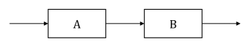
(a) The serial topology, as proposed in [6] or further discussed e.g. in [8]. The subsystem A manipulates values, before passing them further to subsystem B, that computes the actual results.

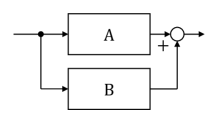
(b) The parallel topology, as proposed in [6] or further discussed e.g. in [8]. The model $B$ learns for the residuals of model $A$ and adds them to the common result.

Figure 1: Serial and parallel combination of models (in hybrid modeling).

However, it is quite easy to show, that the proposed structures are often not feasible in the real application, in the sense that no model inference is possible without further methodological adaptions. This is because of algebraic loops (s. fig. 2(a)) and impeded event-handling (s. fig. 2(b)) of the CM.

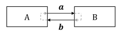
(a) For models $A$ and $B$ with algebraic relation between inputs and outputs (like for example FFNNs), algebraic loops can easily be constructed by connecting both models cyclically. Without handling these algebraic loops, the resulting CM can’t be forward or backward evaluated correctly.

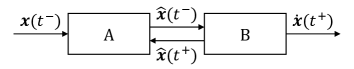
(b) Discontinuous models change their state locally. In this example, model $A$ maps the state on the left side of a discontinuity $\bm{x}(t^{-})$ to $\hat{\bm{x}}(t^{-})$. Model $B$ updates the local state $\hat{\bm{x}}(t^{-})$ discontinuously to $\hat{\bm{x}}(t^{+})$, this new local state must be propagated backwards through model $A$ to obtain a new global state $\bm{x}(t^{+})$.

Figure 2: Scenarios, where state of the art hybrid modeling fails.

The reason behind is, that the current state of the art captures the theoretical possibilities of model combination, but lacks to make statements on the mathematical consequences of the model combination, like e.g. the solvability of the CM. The topic of model combination must be investigated on a mathematical level ob abstraction, considering the types and meanings of systems of equations that can occur during modeling dynamical systems. In the introduced context, this step has not yet been taken to the knowledge of the authors. On top of that, the combination of models in a learnable way instead of statically connecting them, as well as the mathematical consequences of this learnable connection are also not studied yet.

3 Deriving HUDA-ODEs

As stated, a common interface for dynamical system models is needed in order to discuss the combinability of such. In the following, the class of mixed hybrid universal discrete algebraic ordinary differential equations (HUDA-ODEs), that is able to express the considered model types, is derived step by step. A more detailed introduction and inference algorithm is discussed in a parallel contribution that is currently prepared. We start with the foundation of an ODE, that is capable of describing arbitrary dynamical processes:

$$\dot{\bm{x}}(t)=\bm{f}(\bm{x}(t),\bm{p},t)$$ (1)

The ODE depends on the system state $\bm{x}$, parameter vector $\bm{p}$ and time $t$. Because $\bm{f}$ may also include universal approximators, one might also refer to it as universal ordinary differential equation (UODE) as introduced in [11]. However, we don’t use the UA as function argument, to allow for a more versatile combination. To further allow for modeling discontinuous (or hybrid) systems, the UODE can be extended to the hybrid UODE by providing an event condition function $\bm{c}$, indicating events by zero crossings:

$$\bm{z}(t)=\bm{c}(\bm{x}(t),\bm{p},t)$$ (2)

Further, the event affect function $\bm{a}$ performs the state change by event. The state after the event affect is expressed as $\bm{x}(t^{+})$, the state before the event affect as $\bm{x}(t^{-})$:

$$\bm{x}(t^{+})=\bm{a}(\bm{x}(t^{-}),\bm{p},t^{-})$$ (3)

To express algebraic mappings (like we like to do for example in FFNNs), it is common to augment (U)ODEs by an algebraic output equation $\bm{g}$:

$$\bm{y}(t)=\bm{g}(\bm{x}(t),\bm{p},t)$$ (4)

Further, discrete systems, that only change for discrete points in time (like RNNs), need to be considered. The state vector $\bm{x}$ can be separated into the continuous state $\bm{x}_{c}$, that changes continuously over time (by the given derivative in $\bm{f}$), and the discrete state $\bm{x}_{d}$, that changes only at event instances (so inside of the function $\bm{a}$). The original equation $\bm{f}$ (s. equation 1) can therefore be separated into two equations and be reformulated:

$$\dot{\bm{x}}(t)=\begin{bmatrix}\dot{\bm{x}}_{c}(t)\\ \dot{\bm{x}}_{d}(t)\end{bmatrix}=\begin{bmatrix}\bm{f}(\bm{x}_{c}(t),\bm{x}_{d}(t),\bm{p},t)\\ \bm{0}\end{bmatrix}$$ (5)

Finally, the system can be modeled to depend on external inputs $\bm{u}$. Technically, inputs can be interpreted as parameters (constant), continuous states (if the derivative is known), implemented as discrete states that are changed by time-events or the input equation (if known) can be added to the system of equations, so that the system boundary is extended (and no explicitly defined input is needed). The complete mixed hybrid universal discrete algebraic (HUDA)-ODE states:

$$\begin{bmatrix}\dot{\bm{x}}_{c}(t)\\ \dot{\bm{x}}_{d}(t)\\ \bm{y}(t)\\ \bm{z}(t)\\ \bm{x}(t^{+})\end{bmatrix}=\begin{bmatrix}\bm{f}(\bm{x}_{c}(t),\bm{x}_{d}(t),\bm{u}(t),\bm{p},t)\\ \bm{0}\\ \bm{g}(\bm{x}_{c}(t),\bm{x}_{d}(t),\bm{u}(t),\bm{p},t)\\ \bm{c}(\bm{x}_{c}(t),\bm{x}_{d}(t),\bm{u}(t),\bm{p},t)\\ \bm{a}(\bm{x}_{c}(t^{-}),\bm{x}_{d}(t^{-}),\bm{u}(t^{-}),\bm{p},t^{-})\end{bmatrix}$$ (6)

The HUDA-ODE provides a definition for a model interface consisting of five systems of equations with associated meaning. There are no assumptions regarding the origin of the equations, they might be derived from first principles or be machine learning models (or both). Except for the ODE $\bm{f}$, all systems of equations are pure algebraic equations. If $\dot{\bm{x}}_{c}$ is interpreted as unknown (instead of a derivative), even equation $\bm{f}$ can be handled as an algebraic equation. This is an important insight for the next section concerning the combinability of HUDA-ODEs.

4 Combining HUDA-ODEs

Before discussing the combinability of HUDA-ODEs, some basic principles that lead to a simplified discussion are defined:

• It is sufficient to discuss the combination of only two algebraic systems, if this leads to an algebraic system again. This way, one can easily extend the concept to the arbitrary case of combining multiple algebraic systems.

• It is sufficient to consider only a single vectorial input $\bm{u}$ and single vectorial output $\bm{y}$, because multiple inputs/outputs can be concatenated into a single vector. The same applies to multiple systems of equations, they can be concatenated into a single one.

As a consequence, any HUDA-ODE can be expressed as single system of algebraic equations with single vectorial input and single vectorial output, which makes the following statements for systems of algebraic equations applicable.

4.1 Topology: Generic

The combination of two algebraic subsystems $\bm{f}_{a}$ and $\bm{f}_{b}$ (note, that this could be any of $\bm{f}$, $\bm{g}$, $\bm{c}$ or $\bm{a}$ of a HUDA-ODE, a subset or even all of them) into the new algebraic equation $\bm{f}_{z}$ can be mathematically expressed as the concatenation of the two equations, as in fig. 3. However, new unknowns for the inputs $\bm{u}_{a}$ and $\bm{u}_{b}$ and the output $\bm{y}_{z}$ are introduced.

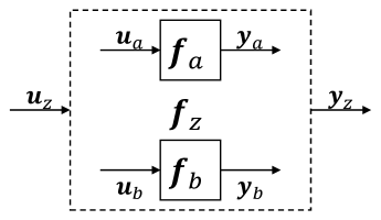
Figure 3: Two algebraic subsystems $\bm{f}_{a}$ and $\bm{f}_{b}$ can be combined to a single one $\bm{f}_{z}$. Because there are new unknowns $\bm{u}_{a}$, $\bm{u}_{b}$, $\bm{y}_{z}$ introduced, the system is not well-posed. This can be seen from the missing connections between the outer input $\bm{u}_{z}$ and output $\bm{y}_{z}$ and the inner inputs $\bm{u}_{a}$ and $\bm{u}_{b}$ and outputs $\bm{y}_{a}$ and $\bm{y}_{b}$.

The concatenated system states:

$$\begin{bmatrix}\bm{y}_{a}\\ \bm{y}_{b}\end{bmatrix}=\begin{bmatrix}\bm{f}_{a}(\bm{u}_{a})\\ \bm{f}_{b}(\bm{u}_{b})\end{bmatrix}$$ (7)

To gain a solvable system, three linear equations $\bm{c}_{a}$, $\bm{c}_{b}$ and $\bm{c}_{z}$ can be added to the system of equations, connecting the newly introduced unknowns:

$$\bm{u}_{a}=\bm{c}_{a}(\bm{y}_{a},\bm{y}_{b},\bm{u}_{z})=\bm{W}_{aa}\bm{y}_{a}+\bm{W}_{ab}\bm{y}_{b}+\bm{W}_{az}\bm{u}_{z}\qquad( +\bm{b}_{a})$$ (8)

$$\bm{u}_{b}=\bm{c}_{b}(\bm{y}_{a},\bm{y}_{b},\bm{u}_{z})=\bm{W}_{ba}\bm{y}_{a}+\bm{W}_{bb}\bm{y}_{b}+\bm{W}_{bz}\bm{u}_{z}\qquad( +\bm{b}_{b})$$ (9)

$$\bm{y}_{z}=\bm{c}_{z}(\bm{y}_{a},\bm{y}_{b},\bm{u}_{z})=\bm{W}_{za}\bm{y}_{a}+\bm{W}_{zb}\bm{y}_{b}+\bm{W}_{zz}\bm{u}_{z}\qquad( +\bm{b}_{z})$$ (10)

with connection matrix $\bm{W}\in\mathbb{R}^{n\times m}$ and connection bias $\bm{b}\in\mathbb{R}^{n}$ with $n=|\bm{u}_{a}|+|\bm{u}_{b}|+|\bm{y}_{z}|$ and $m=|\bm{y}_{a}|+|\bm{y}_{b}|+|\bm{u}_{z}|$:

$$\bm{W}=\hbox{}\vbox{\kern 0.86108pt\hbox{$\kern 0.0pt\kern 2.5pt\kern-5.0pt\left[\kern 0.0pt\kern-2.5pt\kern-5.55557pt\vbox{\kern-0.86108pt\vbox{\vbox{ \halign{\kern\arraycolsep\hfil\@arstrut$\kbcolstyle#$\hfil\kern\arraycolsep& \kern\arraycolsep\hfil$\@kbrowstyle#$\ifkbalignright\relax\else\hfil\fi\kern\arraycolsep&& \kern\arraycolsep\hfil$\@kbrowstyle#$\ifkbalignright\relax\else\hfil\fi\kern\arraycolsep\cr 5.0pt\hfil\@arstrut$\scriptstyle~{}$\hfil\kern 5.0pt&5.0pt\hfil$\scriptstyle\bm{y}_{a}$\hfil\kern 5.0pt&5.0pt\hfil$\scriptstyle\bm{y}_{b}$\hfil\kern 5.0pt&5.0pt\hfil$\scriptstyle\bm{u}_{z}\\\bm{u}_{a}$\hfil\kern 5.0pt&5.0pt\hfil$\scriptstyle\bm{W}_{aa}$\hfil\kern 5.0pt&5.0pt\hfil$\scriptstyle\bm{W}_{ab}$\hfil\kern 5.0pt&5.0pt\hfil$\scriptstyle\bm{W}_{az}\\\bm{u}_{b}$\hfil\kern 5.0pt&5.0pt\hfil$\scriptstyle\bm{W}_{ba}$\hfil\kern 5.0pt&5.0pt\hfil$\scriptstyle\bm{W}_{bb}$\hfil\kern 5.0pt&5.0pt\hfil$\scriptstyle\bm{W}_{bz}\\\bm{y}_{z}$\hfil\kern 5.0pt&5.0pt\hfil$\scriptstyle\bm{W}_{za}$\hfil\kern 5.0pt&5.0pt\hfil$\scriptstyle\bm{W}_{zb}$\hfil\kern 5.0pt&5.0pt\hfil$\scriptstyle\bm{W}_{zz}\\$\hfil\kern 5.0pt\crcr}}}}\right]$}}\qquad\bm{b}=\hbox{}\vbox{\kern 0.86108pt\hbox{$\kern 0.0pt\kern 2.5pt\kern-5.0pt\left[\kern 0.0pt\kern-2.5pt\kern-5.55557pt\vbox{\kern-0.86108pt\vbox{\vbox{ \halign{\kern\arraycolsep\hfil\@arstrut$\kbcolstyle#$\hfil\kern\arraycolsep& \kern\arraycolsep\hfil$\@kbrowstyle#$\ifkbalignright\relax\else\hfil\fi\kern\arraycolsep&& \kern\arraycolsep\hfil$\@kbrowstyle#$\ifkbalignright\relax\else\hfil\fi\kern\arraycolsep\cr 5.0pt\hfil\@arstrut$\scriptstyle~{}$\hfil\kern 5.0pt&5.0pt\hfil$\scriptstyle~{}\\\bm{u}_{a}$\hfil\kern 5.0pt&5.0pt\hfil$\scriptstyle\bm{b}_{a}\\\bm{u}_{b}$\hfil\kern 5.0pt&5.0pt\hfil$\scriptstyle\bm{b}_{b}\\\bm{y}_{z}$\hfil\kern 5.0pt&5.0pt\hfil$\scriptstyle\bm{b}_{z}\\$\hfil\kern 5.0pt\crcr}}}}\right]$}}$$ (11)

These new linear equations based on the connection matrix $\bm{W}$ and bias $\bm{b}$ are fully differentiable regarding $\bm{W}$ and $\bm{b}$ (which is a prerequisite for gradient based optimization) and can be used in multiple ways:

1. The entries of the matrix $\bm{W}$ can be set to identify a connection ($1$) or no connection ($0$) between two variables, while keeping the bias $\bm{b}$ at zeros. This is the common understanding of a connection matrix.

2. The entries of $\bm{W}$ and $\bm{b}$ can be initialized with real values. This way, the equations can be used as pre- and post-processing layers as proposed in [12], to scale and shift data between the combined models to an appropriate value range.

3. The parameters can be initialized by applying (a) or (b) and be further optimized together with other parameters. This is done by appending the parameter vector of the resulting HUDA-ODE. The resulting structure is capable of describing arbitrary connections between two given algebraic subsystems or HUDA-ODEs respectively.

Note, that these connection equations are able to express concatenation, as well as addition of signals, dependent on the chosen dimension of input $\bm{u}_{z}$ and output $\bm{y}_{z}$. Further gates, as in [12], can be implemented if $\bm{W}_{za}$ and $\bm{W}_{zb}$ are trainable parameters. Equations 7, 8, 9 and 10 can be concatenated to obtain the complete and balanced combined system with the following dependency matrix $\bm{D}$:

$$\bm{D}=\hbox{}\vbox{\kern 0.86108pt\hbox{$\kern 0.0pt\kern 2.5pt\kern-5.0pt\left[\kern 0.0pt\kern-2.5pt\kern-5.55557pt\vbox{\kern-0.86108pt\vbox{\vbox{ \halign{\kern\arraycolsep\hfil\@arstrut$\kbcolstyle#$\hfil\kern\arraycolsep& \kern\arraycolsep\hfil$\@kbrowstyle#$\ifkbalignright\relax\else\hfil\fi\kern\arraycolsep&& \kern\arraycolsep\hfil$\@kbrowstyle#$\ifkbalignright\relax\else\hfil\fi\kern\arraycolsep\cr 5.0pt\hfil\@arstrut$\scriptstyle~{}$\hfil\kern 5.0pt&5.0pt\hfil$\scriptstyle\bm{y}_{a}$\hfil\kern 5.0pt&5.0pt\hfil$\scriptstyle\bm{y}_{b}$\hfil\kern 5.0pt&5.0pt\hfil$\scriptstyle\bm{u}_{a}$\hfil\kern 5.0pt&5.0pt\hfil$\scriptstyle\bm{u}_{b}$\hfil\kern 5.0pt&5.0pt\hfil$\scriptstyle\bm{y}_{z}\\\bm{f}_{a}$\hfil\kern 5.0pt&5.0pt\hfil$\scriptstyle\underline{\bm{I}}$\hfil\kern 5.0pt&5.0pt\hfil$\scriptstyle\bm{0}$\hfil\kern 5.0pt&5.0pt\hfil$\scriptstyle\bm{D}_{a}$\hfil\kern 5.0pt&5.0pt\hfil$\scriptstyle\bm{0}$\hfil\kern 5.0pt&5.0pt\hfil$\scriptstyle\bm{0}\\\bm{f}_{b}$\hfil\kern 5.0pt&5.0pt\hfil$\scriptstyle\bm{0}$\hfil\kern 5.0pt&5.0pt\hfil$\scriptstyle\underline{\bm{I}}$\hfil\kern 5.0pt&5.0pt\hfil$\scriptstyle\bm{0}$\hfil\kern 5.0pt&5.0pt\hfil$\scriptstyle\bm{D}_{b}$\hfil\kern 5.0pt&5.0pt\hfil$\scriptstyle\bm{0}\\\bm{c}_{a}$\hfil\kern 5.0pt&5.0pt\hfil$\scriptstyle\bm{W}_{aa}$\hfil\kern 5.0pt&5.0pt\hfil$\scriptstyle\bm{W}_{ab}$\hfil\kern 5.0pt&5.0pt\hfil$\scriptstyle\underline{\bm{I}}$\hfil\kern 5.0pt&5.0pt\hfil$\scriptstyle\bm{0}$\hfil\kern 5.0pt&5.0pt\hfil$\scriptstyle\bm{0}\\\bm{c}_{b}$\hfil\kern 5.0pt&5.0pt\hfil$\scriptstyle\bm{W}_{ba}$\hfil\kern 5.0pt&5.0pt\hfil$\scriptstyle\bm{W}_{bb}$\hfil\kern 5.0pt&5.0pt\hfil$\scriptstyle\bm{0}$\hfil\kern 5.0pt&5.0pt\hfil$\scriptstyle\underline{\bm{I}}$\hfil\kern 5.0pt&5.0pt\hfil$\scriptstyle\bm{0}\\\bm{c}_{z}$\hfil\kern 5.0pt&5.0pt\hfil$\scriptstyle\bm{W}_{za}$\hfil\kern 5.0pt&5.0pt\hfil$\scriptstyle\bm{W}_{zb}$\hfil\kern 5.0pt&5.0pt\hfil$\scriptstyle\bm{0}$\hfil\kern 5.0pt&5.0pt\hfil$\scriptstyle\bm{0}$\hfil\kern 5.0pt&5.0pt\hfil$\scriptstyle\underline{\bm{I}}\\$\hfil\kern 5.0pt\crcr}}}}\right]$}}$$ (12)

The dependency matrix $\bm{D}$ holds the unknown variables in columns and the equations in rows. Note, that only a part of the connection matrix $\bm{W}$ is included, because the last column of $\bm{W}$ refers to the known variable $\bm{u}_{z}$. Further, the dependency matrices of the subsystems to be combined $\bm{D}_{a}$ and $\bm{D}_{b}$ are included. Without further arrangements and for non-trivial dependency matrices $\bm{D}_{a}\neq\bm{0}$ and $\bm{D}_{b}\neq\bm{0}$, the system behind $\bm{D}$ contains algebraic loops. This can easily be proven by performing a block lower triangular (BLT) transformation that is not possible, because all rows contain at least two non-zero entries. Technically, algebraic loops are not an issue but require appropriate handling by identification (e.g. Tarjan’s algorithm [13]) and solving (e.g. Newton’s method for solving nonlinear systems of equations). In case of optimizing the parameters of $\bm{W}$, these steps need to be done online, which is quite costly in terms of computational performance. Here, a topology free of algebraic loops might be desirable and is therefore derived in the following.

4.2 Topology: PSD

To prevent algebraic loops, it is clear that for unknown $\bm{D}_{a}$ and $\bm{D}_{b}$, connections of the equation blocks $\bm{f}_{a}$ and $\bm{f}_{b}$ with themselves must be prohibited, which results in $\bm{W}_{aa}=\bm{W}_{bb}=\bm{0}$. Further, because $\bm{D}_{a}$ and $\bm{D}_{b}$ are assumed non-zero, exactly two meaningful cases remain, further referred to as case (a) and case (b), where a system free of algebraic loops can be constructed (so a successful BLT transform is possible):

1. $\bm{W}_{aa}=\bm{W}_{bb}=\bm{W}_{ab}=\bm{0}$ (see the following deduction) or

2. $\bm{W}_{aa}=\bm{W}_{bb}=\bm{W}_{ba}=\bm{0}$ (see appendix section A.1)

Both cases of this topology can be visualized as in fig. 4. Because this topology features parallel (P), sequential (S) and direct feed through (DFT) (D) characteristics, it can be referred to as topology PSD.

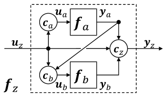
(a) $\bm{f}_{a}$ is evaluated before $\bm{f}_{b}$, so $\bm{W}_{ab}=\bm{0}$.

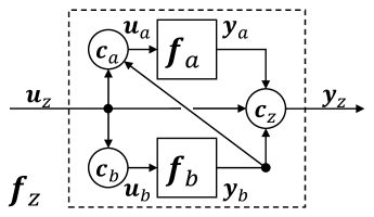
(b) $\bm{f}_{b}$ is evaluated before $\bm{f}_{a}$, so $\bm{W}_{ba}=\bm{0}$.

Figure 4: Two cases (a) and (b) of the PSD topology, the most generic loop-free combination of two algebraic subsystems $\bm{f}_{a}$ and $\bm{f}_{b}$ into the new system $\bm{f}_{z}$. One subsystem is evaluated first, then the other subsystem is evaluated based on the intermediate results of the first one, as well as on the original input $\bm{u}_{z}$. The final system output depends on results from both subsystems and the DFT of the system input $\bm{u}_{z}$, which can be interpreted as residual connection. Each arrow corresponds to a part of the connection matrix $\bm{W}$. Further, the connection equations $\bm{c}_{a}$, $\bm{c}_{b}$ and $\bm{c}_{z}$ are visualized.

Case (a) of the PSD topology leads to the connection matrix:

$$\bm{W}_{PSD}=\hbox{}\vbox{\kern 0.86108pt\hbox{$\kern 0.0pt\kern 2.5pt\kern-5.0pt\left[\kern 0.0pt\kern-2.5pt\kern-5.55557pt\vbox{\kern-0.86108pt\vbox{\vbox{ \halign{\kern\arraycolsep\hfil\@arstrut$\kbcolstyle#$\hfil\kern\arraycolsep& \kern\arraycolsep\hfil$\@kbrowstyle#$\ifkbalignright\relax\else\hfil\fi\kern\arraycolsep&& \kern\arraycolsep\hfil$\@kbrowstyle#$\ifkbalignright\relax\else\hfil\fi\kern\arraycolsep\cr 5.0pt\hfil\@arstrut$\scriptstyle~{}$\hfil\kern 5.0pt&5.0pt\hfil$\scriptstyle\bm{y}_{a}$\hfil\kern 5.0pt&5.0pt\hfil$\scriptstyle\bm{y}_{b}$\hfil\kern 5.0pt&5.0pt\hfil$\scriptstyle\bm{u}_{z}\\\bm{c}_{a}$\hfil\kern 5.0pt&5.0pt\hfil$\scriptstyle\bm{0}$\hfil\kern 5.0pt&5.0pt\hfil$\scriptstyle\bm{0}$\hfil\kern 5.0pt&5.0pt\hfil$\scriptstyle\bm{W}_{az}\\\bm{c}_{b}$\hfil\kern 5.0pt&5.0pt\hfil$\scriptstyle\bm{W}_{ba}$\hfil\kern 5.0pt&5.0pt\hfil$\scriptstyle\bm{0}$\hfil\kern 5.0pt&5.0pt\hfil$\scriptstyle\bm{W}_{bz}\\\bm{c}_{z}$\hfil\kern 5.0pt&5.0pt\hfil$\scriptstyle\bm{W}_{za}$\hfil\kern 5.0pt&5.0pt\hfil$\scriptstyle\bm{W}_{zb}$\hfil\kern 5.0pt&5.0pt\hfil$\scriptstyle\bm{W}_{zz}\\$\hfil\kern 5.0pt\crcr}}}}\right]$}}$$ (13)

For the PSD topology, the system incidence matrix for case (a) can be transformed to BLT form:

$$\bm{D}_{PSD}=\hbox{}\vbox{\kern 0.86108pt\hbox{$\kern 0.0pt\kern 2.5pt\kern-5.0pt\left[\kern 0.0pt\kern-2.5pt\kern-5.55557pt\vbox{\kern-0.86108pt\vbox{\vbox{ \halign{\kern\arraycolsep\hfil\@arstrut$\kbcolstyle#$\hfil\kern\arraycolsep& \kern\arraycolsep\hfil$\@kbrowstyle#$\ifkbalignright\relax\else\hfil\fi\kern\arraycolsep&& \kern\arraycolsep\hfil$\@kbrowstyle#$\ifkbalignright\relax\else\hfil\fi\kern\arraycolsep\cr 5.0pt\hfil\@arstrut$\scriptstyle~{}$\hfil\kern 5.0pt&5.0pt\hfil$\scriptstyle\bm{y}_{a}$\hfil\kern 5.0pt&5.0pt\hfil$\scriptstyle\bm{y}_{b}$\hfil\kern 5.0pt&5.0pt\hfil$\scriptstyle\bm{u}_{a}$\hfil\kern 5.0pt&5.0pt\hfil$\scriptstyle\bm{u}_{b}$\hfil\kern 5.0pt&5.0pt\hfil$\scriptstyle\bm{y}_{z}\\\bm{f}_{a}$\hfil\kern 5.0pt&5.0pt\hfil$\scriptstyle\underline{\bm{I}}$\hfil\kern 5.0pt&5.0pt\hfil$\scriptstyle\bm{0}$\hfil\kern 5.0pt&5.0pt\hfil$\scriptstyle\bm{D}_{a}$\hfil\kern 5.0pt&5.0pt\hfil$\scriptstyle\bm{0}$\hfil\kern 5.0pt&5.0pt\hfil$\scriptstyle\bm{0}\\\bm{f}_{b}$\hfil\kern 5.0pt&5.0pt\hfil$\scriptstyle\bm{0}$\hfil\kern 5.0pt&5.0pt\hfil$\scriptstyle\underline{\bm{I}}$\hfil\kern 5.0pt&5.0pt\hfil$\scriptstyle\bm{0}$\hfil\kern 5.0pt&5.0pt\hfil$\scriptstyle\bm{D}_{b}$\hfil\kern 5.0pt&5.0pt\hfil$\scriptstyle\bm{0}\\\bm{c}_{a}$\hfil\kern 5.0pt&5.0pt\hfil$\scriptstyle\bm{0}$\hfil\kern 5.0pt&5.0pt\hfil$\scriptstyle\bm{0}$\hfil\kern 5.0pt&5.0pt\hfil$\scriptstyle\underline{\bm{I}}$\hfil\kern 5.0pt&5.0pt\hfil$\scriptstyle\bm{0}$\hfil\kern 5.0pt&5.0pt\hfil$\scriptstyle\bm{0}\\\bm{c}_{b}$\hfil\kern 5.0pt&5.0pt\hfil$\scriptstyle\bm{W}_{ba}$\hfil\kern 5.0pt&5.0pt\hfil$\scriptstyle\bm{0}$\hfil\kern 5.0pt&5.0pt\hfil$\scriptstyle\bm{0}$\hfil\kern 5.0pt&5.0pt\hfil$\scriptstyle\underline{\bm{I}}$\hfil\kern 5.0pt&5.0pt\hfil$\scriptstyle\bm{0}\\\bm{c}_{z}$\hfil\kern 5.0pt&5.0pt\hfil$\scriptstyle\bm{W}_{za}$\hfil\kern 5.0pt&5.0pt\hfil$\scriptstyle\bm{W}_{zb}$\hfil\kern 5.0pt&5.0pt\hfil$\scriptstyle\bm{0}$\hfil\kern 5.0pt&5.0pt\hfil$\scriptstyle\bm{0}$\hfil\kern 5.0pt&5.0pt\hfil$\scriptstyle\underline{\bm{I}}\\$\hfil\kern 5.0pt\crcr}}}}\right]$}}\mathrel{\overset{\makebox[0.0pt]{\mbox{BLT}}}{=}}\hbox{}\vbox{\kern 0.86108pt\hbox{$\kern 0.0pt\kern 2.5pt\kern-5.0pt\left[\kern 0.0pt\kern-2.5pt\kern-5.55557pt\vbox{\kern-0.86108pt\vbox{\vbox{ \halign{\kern\arraycolsep\hfil\@arstrut$\kbcolstyle#$\hfil\kern\arraycolsep& \kern\arraycolsep\hfil$\@kbrowstyle#$\ifkbalignright\relax\else\hfil\fi\kern\arraycolsep&& \kern\arraycolsep\hfil$\@kbrowstyle#$\ifkbalignright\relax\else\hfil\fi\kern\arraycolsep\cr 5.0pt\hfil\@arstrut$\scriptstyle~{}$\hfil\kern 5.0pt&5.0pt\hfil$\scriptstyle\bm{u}_{a}$\hfil\kern 5.0pt&5.0pt\hfil$\scriptstyle\bm{y}_{a}$\hfil\kern 5.0pt&5.0pt\hfil$\scriptstyle\bm{u}_{b}$\hfil\kern 5.0pt&5.0pt\hfil$\scriptstyle\bm{y}_{b}$\hfil\kern 5.0pt&5.0pt\hfil$\scriptstyle\bm{y}_{z}\\\bm{c}_{a}$\hfil\kern 5.0pt&5.0pt\hfil$\scriptstyle\underline{\bm{I}}$\hfil\kern 5.0pt&5.0pt\hfil$\scriptstyle\bm{0}$\hfil\kern 5.0pt&5.0pt\hfil$\scriptstyle\bm{0}$\hfil\kern 5.0pt&5.0pt\hfil$\scriptstyle\bm{0}$\hfil\kern 5.0pt&5.0pt\hfil$\scriptstyle\bm{0}\\\bm{f}_{a}$\hfil\kern 5.0pt&5.0pt\hfil$\scriptstyle\bm{D}_{a}$\hfil\kern 5.0pt&5.0pt\hfil$\scriptstyle\underline{\bm{I}}$\hfil\kern 5.0pt&5.0pt\hfil$\scriptstyle\bm{0}$\hfil\kern 5.0pt&5.0pt\hfil$\scriptstyle\bm{0}$\hfil\kern 5.0pt&5.0pt\hfil$\scriptstyle\bm{0}\\\bm{c}_{b}$\hfil\kern 5.0pt&5.0pt\hfil$\scriptstyle\bm{0}$\hfil\kern 5.0pt&5.0pt\hfil$\scriptstyle\bm{W}_{ba}$\hfil\kern 5.0pt&5.0pt\hfil$\scriptstyle\underline{\bm{I}}$\hfil\kern 5.0pt&5.0pt\hfil$\scriptstyle\bm{0}$\hfil\kern 5.0pt&5.0pt\hfil$\scriptstyle\bm{0}\\\bm{f}_{b}$\hfil\kern 5.0pt&5.0pt\hfil$\scriptstyle\bm{0}$\hfil\kern 5.0pt&5.0pt\hfil$\scriptstyle\bm{0}$\hfil\kern 5.0pt&5.0pt\hfil$\scriptstyle\bm{D}_{b}$\hfil\kern 5.0pt&5.0pt\hfil$\scriptstyle\underline{\bm{I}}$\hfil\kern 5.0pt&5.0pt\hfil$\scriptstyle\bm{0}\\\bm{c}_{z}$\hfil\kern 5.0pt&5.0pt\hfil$\scriptstyle\bm{0}$\hfil\kern 5.0pt&5.0pt\hfil$\scriptstyle\bm{W}_{za}$\hfil\kern 5.0pt&5.0pt\hfil$\scriptstyle\bm{0}$\hfil\kern 5.0pt&5.0pt\hfil$\scriptstyle\bm{W}_{zb}$\hfil\kern 5.0pt&5.0pt\hfil$\scriptstyle\underline{\bm{I}}\\$\hfil\kern 5.0pt\crcr}}}}\right]$}}$$ (14)

The proposed PSD topology allows for the combination of two algebraic subsystems (with unknown internal dependencies $\bm{D}_{a}$ and $\bm{D}_{b}$) in the most generic way, concerning that the resulting system is free of algebraic loops by design. The only decision that must be made in advance, is on which subsystem is evaluated first, which corresponds to the two discussed cases (a) and (b).

4.3 Derived Topologies

In this section we show, that more simple topologies - including the known concepts of serial and parallel structure (referred to as P and S) - can be further derived from the PSD topology by setting parts of the connection matrix $\bm{W}$ to zeros.

Table 1: Occupancy of connection matrices for the different topologies for case (a).
Legend: $\times$ = true, $\circ$ = false

P	S	D	$\bm{W}_{az}\neq\bm{0}$	$\bm{W}_{ba}\neq\bm{0}$	$\bm{W}_{bz}\neq\bm{0}$	$\bm{W}_{za}\neq\bm{0}$	$\bm{W}_{zb}\neq\bm{0}$	$\bm{W}_{zz}\neq\bm{0}$
$\times$	$\times$	$\times$	$\times$	$\times$	$\times$	$\times$	$\times$	$\times$
$\times$	$\times$	$\circ$	$\times$	$\times$	$\times$	$\times$	$\times$	$\circ$
$\times$	$\circ$	$\times$	$\times$	$\circ$	$\times$	$\times$	$\times$	$\times$
$\times$	$\circ$	$\circ$	$\times$	$\circ$	$\times$	$\times$	$\times$	$\circ$
$\circ$	$\times$	$\times$	$\times$	$\times$	$\circ$	$\circ$	$\times$	$\times$
$\circ$	$\times$	$\circ$	$\times$	$\times$	$\circ$	$\circ$	$\times$	$\circ$
$\circ$	$\circ$	$\times$	$\circ$	$\circ$	$\circ$	$\circ$	$\circ$	$\times$
$\circ$	$\circ$	$\circ$	$\circ$	$\circ$	$\circ$	$\circ$	$\circ$	$\circ$

In table 1 and the following, topologies are distinguished by naming only the attributes (or connections) that are true (or non-zero). For example, PS identifies the topology which uses P(arallel) and S(equential) layout, but not the D(FT) connection. The topology with only zero connections (the last row of table 1) is not of practical relevance and not further investigated.

4.4 Local state affect function

Event handling of combined algebraic systems is challenging, because of the local state of the subsystem. This results in a local event affect function: The new state for after the event instance corresponds to the local state definition of the subsystem that triggered the event. This local state does not match the global state of the combined system and can even have another dimension, because of the introduced linear connection equations. As a consequence, the global state must be determined for a given local state at any event, this determination might further not have a unique solution, because the subsystems might not be invertible.

Technically, at the time of event handling, the causalization of the system changes: The local state of the event subsystem (that is unknown between events and input to the subsystem) becomes known, the global state (that is known and determined by the numerical solver between events) becomes unknown and must be determined by the system of equations. For the example of an event in subsystem $b$ for the PSD-topology case (a), the dependency matrix of the system at event $\bm{D}_{event\_b}$ states:

$$\bm{D}_{event\_b}\mathrel{\overset{\makebox[0.0pt]{\mbox{BLT}}}{=}}\hbox{}\vbox{\kern 0.86108pt\hbox{$\kern 0.0pt\kern 2.5pt\kern-5.0pt\left[\kern 0.0pt\kern-2.5pt\kern-5.55557pt\vbox{\kern-0.86108pt\vbox{\vbox{ \halign{\kern\arraycolsep\hfil\@arstrut$\kbcolstyle#$\hfil\kern\arraycolsep& \kern\arraycolsep\hfil$\@kbrowstyle#$\ifkbalignright\relax\else\hfil\fi\kern\arraycolsep&& \kern\arraycolsep\hfil$\@kbrowstyle#$\ifkbalignright\relax\else\hfil\fi\kern\arraycolsep\cr 5.0pt\hfil\@arstrut$\scriptstyle~{}$\hfil\kern 5.0pt&5.0pt\hfil$\scriptstyle\bm{y}_{b}$\hfil\kern 5.0pt&5.0pt\hfil$\scriptstyle\bm{y}_{a}$\hfil\kern 5.0pt&5.0pt\hfil$\scriptstyle\bm{u}_{a}$\hfil\kern 5.0pt&5.0pt\hfil$\scriptstyle\bm{u}_{z}$\hfil\kern 5.0pt&5.0pt\hfil$\scriptstyle\bm{y}_{z}\\\bm{f}_{b}$\hfil\kern 5.0pt&5.0pt\hfil$\scriptstyle\underline{\bm{I}}$\hfil\kern 5.0pt&5.0pt\hfil$\scriptstyle\bm{0}$\hfil\kern 5.0pt&5.0pt\hfil$\scriptstyle\bm{0}$\hfil\kern 5.0pt&5.0pt\hfil$\scriptstyle\bm{0}$\hfil\kern 5.0pt&5.0pt\hfil$\scriptstyle\bm{0}\\\bm{c}_{b}$\hfil\kern 5.0pt&5.0pt\hfil$\scriptstyle\bm{0}$\hfil\kern 5.0pt&5.0pt\hfil$\scriptstyle\underline{\bm{W}}_{ba}$\hfil\kern 5.0pt&5.0pt\hfil$\scriptstyle\bm{0}$\hfil\kern 5.0pt&5.0pt\hfil$\scriptstyle\bm{W}_{bz}$\hfil\kern 5.0pt&5.0pt\hfil$\scriptstyle\bm{0}\\\bm{f}_{a}$\hfil\kern 5.0pt&5.0pt\hfil$\scriptstyle\bm{0}$\hfil\kern 5.0pt&5.0pt\hfil$\scriptstyle\bm{I}$\hfil\kern 5.0pt&5.0pt\hfil$\scriptstyle\underline{\bm{D}}_{a}$\hfil\kern 5.0pt&5.0pt\hfil$\scriptstyle\bm{0}$\hfil\kern 5.0pt&5.0pt\hfil$\scriptstyle\bm{0}\\\bm{c}_{a}$\hfil\kern 5.0pt&5.0pt\hfil$\scriptstyle\bm{0}$\hfil\kern 5.0pt&5.0pt\hfil$\scriptstyle\bm{0}$\hfil\kern 5.0pt&5.0pt\hfil$\scriptstyle\bm{I}$\hfil\kern 5.0pt&5.0pt\hfil$\scriptstyle\underline{\bm{W}}_{az}$\hfil\kern 5.0pt&5.0pt\hfil$\scriptstyle\bm{0}\\\bm{c}_{z}$\hfil\kern 5.0pt&5.0pt\hfil$\scriptstyle\bm{W}_{zb}$\hfil\kern 5.0pt&5.0pt\hfil$\scriptstyle\bm{W}_{za}$\hfil\kern 5.0pt&5.0pt\hfil$\scriptstyle\bm{0}$\hfil\kern 5.0pt&5.0pt\hfil$\scriptstyle\bm{W}_{zz}$\hfil\kern 5.0pt&5.0pt\hfil$\scriptstyle\underline{\bm{I}}\\$\hfil\kern 5.0pt\crcr}}}}\right]$}}$$ (15)

Because this system contains an algebraic loop for $\bm{W}_{bz}\neq\bm{0}$, the solution must be obtained by optimization. The optimization residual $\bm{r}_{event\_b}$ is derived by inserting equations $\bm{c}_{a}$, $\bm{f}_{a}$ and $\bm{c}_{b}$ (as obtained by the BLT transform in equation 14) into each other and states:

$$\bm{r}_{event\_b}(\bm{u}_{z})=||\underbrace{\bm{W}_{ba}\bm{f}_{a}(\bm{W}_{az}\bm{u}_{z})}_{\text{by subsystem $a${}}}+\underbrace{\bm{W}_{bz}\bm{u}_{z}}_{\text{by input}}-\bm{u}_{b}||$$ (16)

During solving, it is important to only optimize sensitive entries of $\bm{u}_{z}$, so the entries with non-zero sensitivities for the gradient $\frac{\partial\bm{r}_{event\_b}}{\partial\bm{u}_{z}}$. Otherwise, independent parts of the global state vector might be changed unintentionally. For different edge cases, analytical solutions can be derived for the global state $\bm{u}_{z}$. For example, if $\bm{W}_{bz}=\bm{0}$ and $\bm{W}_{az}$, $\bm{W}_{ba}$ and $\bm{f}_{a}$ are invertible, $\bm{u}_{z}$ can be determined directly (compare to equation 15):

$$\bm{u}_{z}=\bm{W}_{az}^{-1}\bm{f}_{a}^{-1}(\bm{W}_{ba}^{-1}\bm{u}_{b})$$ (17)

Events in subsystem $a$ for case (a) are much more easy to handle, because the new state does not need to be propagated backwards through another subsystem. Handling of an event in the subsystem $a$ is described in the appendix section A.2.

5 Experiment

The contributions of this paper are highlighted at an experimental proof of concept: Different (generic) topologies are deployed, that allow for training arbitrary connections inside a CM, consisting of a FPM in form of an ODE-based simulation model and a MLM in form of an arifical neural network (ANN), together with optimization of parameters of the ANN. The corresponding software library as well as the example script can be found on GitHub.

In the following experiment, the CM (in form of a HUDA-ODE) consists of a FPM and a MLM (both HUDA-ODEs). The FPM represents the well-known bouncing ball in two dimensions ($x$ and $y$) with collision surfaces at $x=\{-1,1\}$ and $y=\{-1,1\}$. Further, ground truth data from a more detailed simulation of the bouncing ball including a simple air friction model is available. The training goal is to match the high-fidelity ground truth data with the CM consisting of the low-fidelity bouncing ball FPM and the MLM. More details about the FPM, MLM, the initialization of connections and further details on the applied training can be found in appendix sec. A.3. To exemplify the presented method, the CM is trained based on the different proposed topologies under identical conditions and results are compared. The $2^{3}=8$ experiments are generated by permutation of the introduced topology attributes: S(equential), P(arallel) and D(FT). All submatrices of the connection matrix $\bm{W}$ are initialized and optimized or set statically according to the chosen topology ($\bm{b}$ is not used in the experiment).

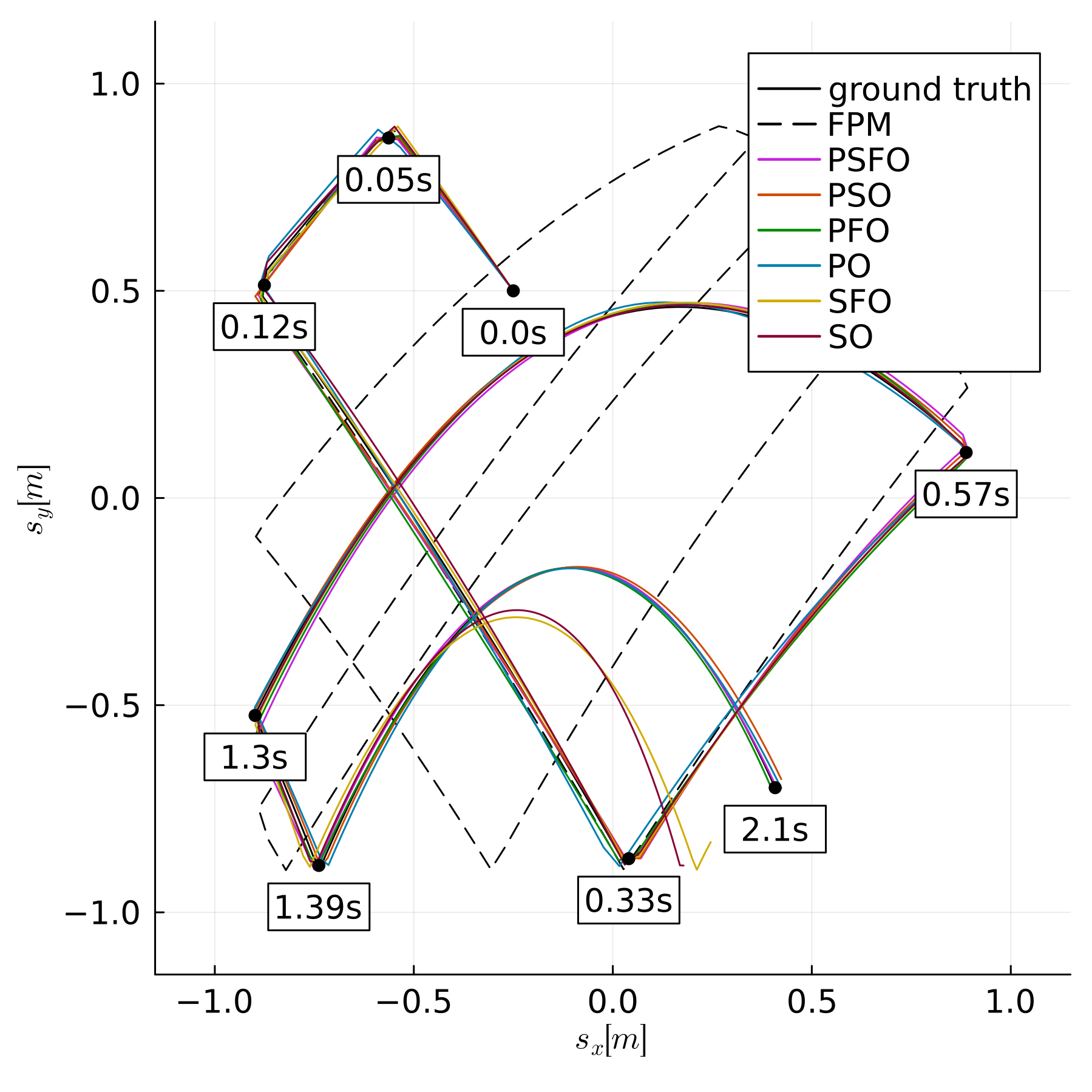
(a) The figure shows the $s_{x}$-$s_{y}$-plane of the ball position on training data. Comparison of the topologies, that succeeded after training. Black (dashed) shows the simulation trajectory of the FPM (without air friction). All trajectories start at ball position $(-0.25,0.5)$. The topologies PSFO, PSO, PFO and PO (different colors) all lay visually above the ground truth trajectory (black), that includes an air friction model that is not present in the FPM. The serial topologies SFO and SO have difficulties to match the data, because of the missing bias $\bm{b}$ in this experiment (that is necessary to compensate for the constant acceleration in $y$ by gravity). These two trajectories also converge, if the trainable bias is applied. A set of solution points is marked with black dots, to track the simulation trajectory over time.

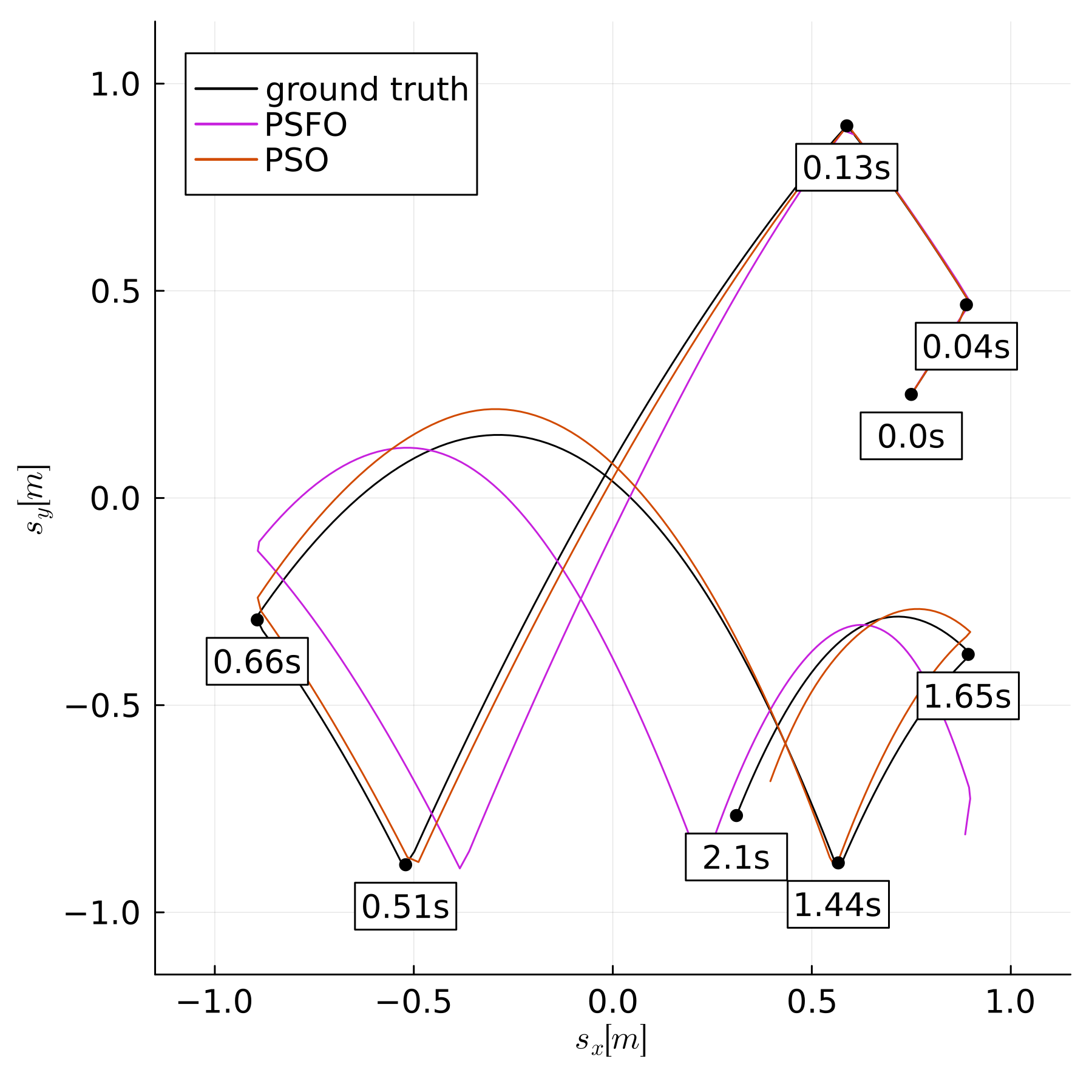
(b) The figure shows the $s_{x}$-$s_{y}$-plane of the ball position on testing data. In this experiment, the ball is initialized at position $(0.75,0.25)$, which is not known from training. Even if the topologies PSFO and PSO both perform very well on training data (compare the left plot), it can be seen that the topology PSFO learned wrong correlations between ball acceleration in $x$ and the ball positions (compare to the visualization of matrix $W_{zz}$ in fig. 6), resulting in too strong damping in direction $x$ on testing data (in which we intentionally changed the sensitive starting positions). The simulation trajectory of PSFO has a larger deviation, compared to the topology PSO, which is not using the DFT and has therefore now access to the non-causal data correlation.

Figure 5: Experimental results.

For a simple interpretation, the connection matrices can be plotted. The results of the topology PSFO and PSO can be investigated in figures 6 and 7. Further results are available in the section A.4. The connection matrices are converted to gray scale (1=white, 0=black). The submatrix identifier and the applied scaling factor is visible as the subplot title.

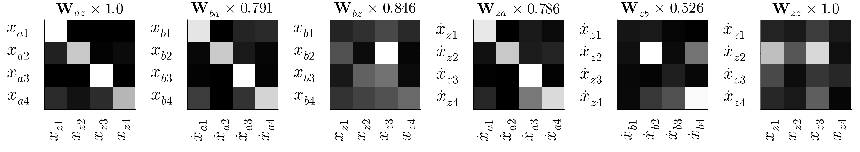
Figure 6: PSFO: The matrices $\bm{W}_{az}$, $\bm{W}_{ba}$ and $\bm{W}_{za}$ are initialized with (noisy) identity, the remaining with (noisy) zeros. All matrix weights are optimized together with the ANN parameters.

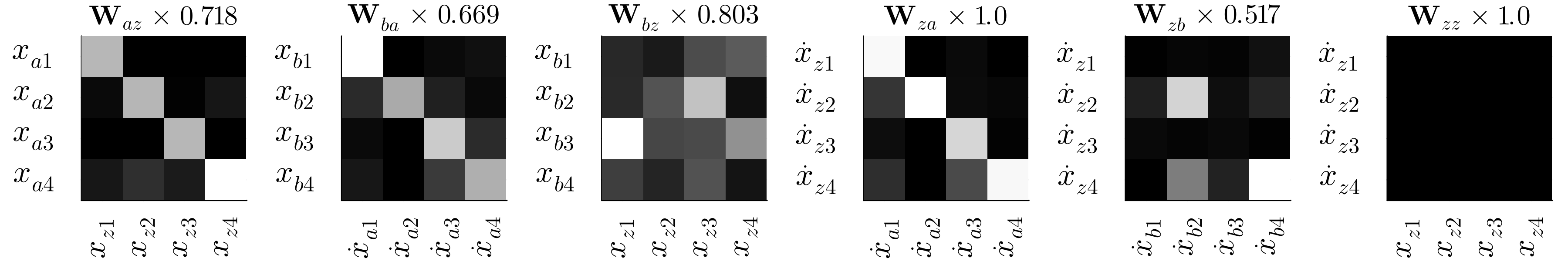
Figure 7: PSO: The matrices $\bm{W}_{az}$, $\bm{W}_{ba}$ and $\bm{W}_{za}$ are initialized with (noisy) identity, the remaining with (noisy) zeros. All matrix weights except $\bm{W}_{zz}$ are optimized together with the ANN parameters.

Interpretation of the PSFO and PSO topologies training results:

$\bm{W}_{az}$

The matrix visualizes the connection between the global system state $\bm{x}_{z}$ (input of CM) and subsystem $a$ state $\bm{x}_{a}$ (input of FPM). For both topologies, it is initialized with (noisy) identity and almost remains in its identity shape, showing a strict connection between the global state and the local state of the FPM.

$\bm{W}_{ba}$

The matrix visualizes the connection between the subsystem $a$ local state derivative $\dot{\bm{x}}_{a}$ (output of FPM) and subsystem $b$ local state $\bm{x}_{b}$ (input of MLM). This corresponds to the serial connection between the FPM and MLM. It is initialized with (noisy) identity and, like $\bm{W}_{az}$, it stays close to its identity shape after training for both topologies. This results in a strong serial connection between subsystem $a$ (output) and $b$ (input).

$\bm{W}_{bz}$

The matrix visualizes the connection between the global system state $\bm{x}_{z}$ (input of CM) and subsystem $b$ local state $\bm{x}_{b}$ (input of MLM). It is initialized with (noisy) zeros. After training, a linear combination of states is used as input to the MLM.

$\bm{W}_{za}$

The matrix visualizes the connection between the subsystem $a$ state derivative $\dot{\bm{x}}_{a}$ (output of FPM) and global state derivative $\dot{\bm{x}}_{z}$ (output of CM). It is initialized with (noisy) identity and remains in an identity like shape. There are only small non-causal deviations. This indicates a strong connection between FPM (output) and global system output, resulting (together with $\bm{W}_{zb}$) in a parallel like structure.

$\bm{W}_{zb}$

The matrix visualizes the connection between the subsystem $b$ state derivative $\dot{\bm{x}}_{b}$ (output of MLM) and global state derivative $\dot{\bm{x}}_{z}$ (output of CM). It is initialized with (noisy) zeros. Mainly, the ball accelerations ($\dot{x}_{b2}$ and $\dot{x}_{b4}$) are connected to the CM output derivative. The expected connections $(2,2)$ and $(4,4)$ being the most prominent, however small cross correlations at $(2,4)$ and $(4,2)$ are present.

$\bm{W}_{zz}$

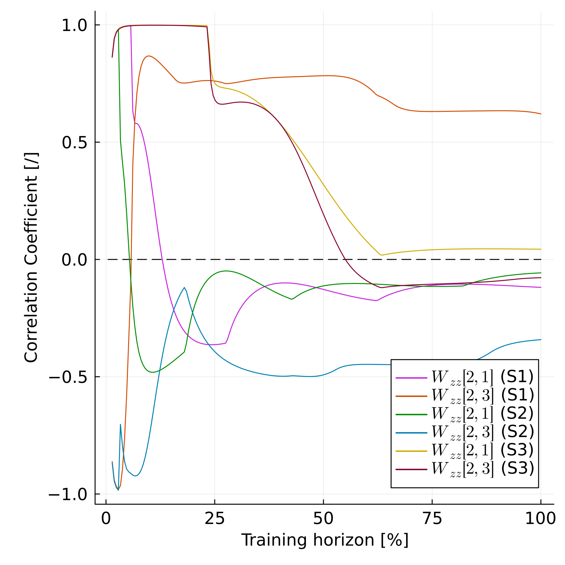
Figure 12: For the PSFO topology, the matrix $\bm{W}_{zz}$ shows hard to interpret learned connections at $(2,1)$ (ball position $x$ and ball acceleration $x$) and $(2,3)$ (ball position $y$ and ball acceleration $x$). Comparing to the equations of the FPM, it can be seen that there are no causalities between the connected variables (the partial derivative between the corresponding variables is zero). However, by investigating the correlation coefficient for the entries $(2,1)$ and $(2,3)$ for the three scenarios ($S1$, $S2$ and $S3$), we find that there are strong correlations (especially during the first quarter of training) between unrelated variables (all plots should converge to zero, black dashed). Particularly noticeable is the connection $\bm{W}_{zz}[2,3]$ in scenarios 1 and 2. In general, unintended correlations often indicate a lack of training data - which is the case in this example.

The matrix visualizes the connection between the global system state $\bm{x}_{z}$ (input of CM) and global state derivative $\dot{\bm{x}}_{z}$ (output of CM). It is initialized with (noisy) zeros, interestingly some unexpected connections can be found here for the PSFO topology, based on non-causal correlations in the very little data set. The strongest ones are at $(2,3)$ and $(2,1)$ (the connection between ball positions and the ball acceleration in $y$), which is obviously non-causal, but can be explained by the correlation anaylysis in the appendix, see figure 12.

In many applications, data is sparse and rare and optimal network architectures unknown. It is shown that in such cases wrong dependencies may be learned. Thus, while providing a method for learning connections between submodels, it is important that using system knowledge in architecture layout is highly desirable. In this example, even if the PSFO topology is able to find a good solution on training data, the PSO topology is less likely to learn for non-causal correlations and offers a much better extrapolation quality on unknown data.

6 Conclusion

In this contribution, we briefly introduced a model interface, the HUDA-ODE, that is able to express dynamic system models from different application areas, like e.g. machine learning (ML), physics and engineering. Further, we discussed, how such models can be combined to obtain a mathematical system that is solvable with or without handling of algebraic loops required. A special event handling routine is necessary for discontinuous combined models and was presented. We found, that the combined model still falls in the class of HUDA-ODE, which offers a great potential for the reuse of methods and code.

The introduced connection parameters $\bm{W}$ and $\bm{b}$ are differentiable and can therefore be learned by gradient based optimization. However, it was also shown that for applications with very limited data (like the example in this contribution), it is target oriented to limit the expressiveness of the applied topology to prevent learning of unintended correlations. Finally, it is important to clarify, that the proposed combination topologies are already realizable within different acausal modeling languages like Modelica [14] and modeling/programming tools like ModelingToolkit.jl [15], as well as causal modeling languages like Simulink [16]. However, most modeling tools are still missing crucial feature implementations to allow for learnable connections (like for example automatic differentiation).

Current and future work covers the development of new methods (and adaption of existing ones) for HUDA-ODEs, for example, training strategies for CMs. We are preparing a parallel contribution, showing that many further state of the art machine learning topologies, like e.g. variational auto encoders, can be expressed as HUDA-ODEs including all presented advantages. Finally, the concept of HUDA-ODEs can be extended to differential equations in general (so HUDA-DEs), instead of restricting it to ODEs.

Abbreviations

ANN

arifical neural network

BLT

block lower triangular

CM

combined model

DFT

direct feed through

FFNN

feed-forward neural network

FPM

first principles model

GPU

graphics processing unit

HUDA

mixed hybrid universal discrete algebraic

MAE

mean absolute error

ML

machine learning

MLM

machine learning model

ODE

ordinary differential equation

RNN

recurrent neural network

SciML

scientific machine learning

UA

universal approximator

UODE

universal ordinary differential equation

Funding

This research was partially funded by the University of Augsburg internal funding project Forschungspotentiale besser nutzen!, we like to thank the university leadership for this opportunity.

Appendix A Appendix / supplemental material

A.1 Incidence matrix: case (b)

Case (b) of the PSD topology leads to the connection matrix:

$$\bm{W}_{PSD}=\hbox{}\vbox{\kern 0.86108pt\hbox{$\kern 0.0pt\kern 2.5pt\kern-5.0pt\left[\kern 0.0pt\kern-2.5pt\kern-5.55557pt\vbox{\kern-0.86108pt\vbox{\vbox{ \halign{\kern\arraycolsep\hfil\@arstrut$\kbcolstyle#$\hfil\kern\arraycolsep& \kern\arraycolsep\hfil$\@kbrowstyle#$\ifkbalignright\relax\else\hfil\fi\kern\arraycolsep&& \kern\arraycolsep\hfil$\@kbrowstyle#$\ifkbalignright\relax\else\hfil\fi\kern\arraycolsep\cr 5.0pt\hfil\@arstrut$\scriptstyle~{}$\hfil\kern 5.0pt&5.0pt\hfil$\scriptstyle\bm{y}_{a}$\hfil\kern 5.0pt&5.0pt\hfil$\scriptstyle\bm{y}_{b}$\hfil\kern 5.0pt&5.0pt\hfil$\scriptstyle\bm{u}_{z}\\\bm{c}_{a}$\hfil\kern 5.0pt&5.0pt\hfil$\scriptstyle\bm{0}$\hfil\kern 5.0pt&5.0pt\hfil$\scriptstyle\bm{W}_{ab}$\hfil\kern 5.0pt&5.0pt\hfil$\scriptstyle\bm{W}_{az}\\\bm{c}_{b}$\hfil\kern 5.0pt&5.0pt\hfil$\scriptstyle\bm{0}$\hfil\kern 5.0pt&5.0pt\hfil$\scriptstyle\bm{0}$\hfil\kern 5.0pt&5.0pt\hfil$\scriptstyle\bm{W}_{bz}\\\bm{c}_{z}$\hfil\kern 5.0pt&5.0pt\hfil$\scriptstyle\bm{W}_{za}$\hfil\kern 5.0pt&5.0pt\hfil$\scriptstyle\bm{W}_{zb}$\hfil\kern 5.0pt&5.0pt\hfil$\scriptstyle\bm{W}_{zz}\\$\hfil\kern 5.0pt\crcr}}}}\right]$}}$$ (18)

For the PSD topology, the system incidence matrix for case (b) can be transformed to BLT form:

$$\bm{D}_{PSD}=\hbox{}\vbox{\kern 0.86108pt\hbox{$\kern 0.0pt\kern 2.5pt\kern-5.0pt\left[\kern 0.0pt\kern-2.5pt\kern-5.55557pt\vbox{\kern-0.86108pt\vbox{\vbox{ \halign{\kern\arraycolsep\hfil\@arstrut$\kbcolstyle#$\hfil\kern\arraycolsep& \kern\arraycolsep\hfil$\@kbrowstyle#$\ifkbalignright\relax\else\hfil\fi\kern\arraycolsep&& \kern\arraycolsep\hfil$\@kbrowstyle#$\ifkbalignright\relax\else\hfil\fi\kern\arraycolsep\cr 5.0pt\hfil\@arstrut$\scriptstyle~{}$\hfil\kern 5.0pt&5.0pt\hfil$\scriptstyle\bm{y}_{a}$\hfil\kern 5.0pt&5.0pt\hfil$\scriptstyle\bm{y}_{b}$\hfil\kern 5.0pt&5.0pt\hfil$\scriptstyle\bm{u}_{a}$\hfil\kern 5.0pt&5.0pt\hfil$\scriptstyle\bm{u}_{b}$\hfil\kern 5.0pt&5.0pt\hfil$\scriptstyle\bm{y}_{z}\\\bm{f}_{a}$\hfil\kern 5.0pt&5.0pt\hfil$\scriptstyle\underline{\bm{I}}$\hfil\kern 5.0pt&5.0pt\hfil$\scriptstyle\bm{0}$\hfil\kern 5.0pt&5.0pt\hfil$\scriptstyle\bm{D}_{a}$\hfil\kern 5.0pt&5.0pt\hfil$\scriptstyle\bm{0}$\hfil\kern 5.0pt&5.0pt\hfil$\scriptstyle\bm{0}\\\bm{f}_{b}$\hfil\kern 5.0pt&5.0pt\hfil$\scriptstyle\bm{0}$\hfil\kern 5.0pt&5.0pt\hfil$\scriptstyle\underline{\bm{I}}$\hfil\kern 5.0pt&5.0pt\hfil$\scriptstyle\bm{0}$\hfil\kern 5.0pt&5.0pt\hfil$\scriptstyle\bm{D}_{b}$\hfil\kern 5.0pt&5.0pt\hfil$\scriptstyle\bm{0}\\\bm{c}_{a}$\hfil\kern 5.0pt&5.0pt\hfil$\scriptstyle\bm{0}$\hfil\kern 5.0pt&5.0pt\hfil$\scriptstyle\bm{W}_{ab}$\hfil\kern 5.0pt&5.0pt\hfil$\scriptstyle\underline{\bm{I}}$\hfil\kern 5.0pt&5.0pt\hfil$\scriptstyle\bm{0}$\hfil\kern 5.0pt&5.0pt\hfil$\scriptstyle\bm{0}\\\bm{c}_{b}$\hfil\kern 5.0pt&5.0pt\hfil$\scriptstyle\bm{0}$\hfil\kern 5.0pt&5.0pt\hfil$\scriptstyle\bm{0}$\hfil\kern 5.0pt&5.0pt\hfil$\scriptstyle\bm{0}$\hfil\kern 5.0pt&5.0pt\hfil$\scriptstyle\underline{\bm{I}}$\hfil\kern 5.0pt&5.0pt\hfil$\scriptstyle\bm{0}\\\bm{c}_{z}$\hfil\kern 5.0pt&5.0pt\hfil$\scriptstyle\bm{W}_{za}$\hfil\kern 5.0pt&5.0pt\hfil$\scriptstyle\bm{W}_{zb}$\hfil\kern 5.0pt&5.0pt\hfil$\scriptstyle\bm{0}$\hfil\kern 5.0pt&5.0pt\hfil$\scriptstyle\bm{0}$\hfil\kern 5.0pt&5.0pt\hfil$\scriptstyle\underline{\bm{I}}\\$\hfil\kern 5.0pt\crcr}}}}\right]$}}\mathrel{\overset{\makebox[0.0pt]{\mbox{BLT}}}{=}}\hbox{}\vbox{\kern 0.86108pt\hbox{$\kern 0.0pt\kern 2.5pt\kern-5.0pt\left[\kern 0.0pt\kern-2.5pt\kern-5.55557pt\vbox{\kern-0.86108pt\vbox{\vbox{ \halign{\kern\arraycolsep\hfil\@arstrut$\kbcolstyle#$\hfil\kern\arraycolsep& \kern\arraycolsep\hfil$\@kbrowstyle#$\ifkbalignright\relax\else\hfil\fi\kern\arraycolsep&& \kern\arraycolsep\hfil$\@kbrowstyle#$\ifkbalignright\relax\else\hfil\fi\kern\arraycolsep\cr 5.0pt\hfil\@arstrut$\scriptstyle~{}$\hfil\kern 5.0pt&5.0pt\hfil$\scriptstyle\bm{u}_{b}$\hfil\kern 5.0pt&5.0pt\hfil$\scriptstyle\bm{y}_{b}$\hfil\kern 5.0pt&5.0pt\hfil$\scriptstyle\bm{u}_{a}$\hfil\kern 5.0pt&5.0pt\hfil$\scriptstyle\bm{y}_{a}$\hfil\kern 5.0pt&5.0pt\hfil$\scriptstyle\bm{y}_{z}\\\bm{c}_{b}$\hfil\kern 5.0pt&5.0pt\hfil$\scriptstyle\underline{\bm{I}}$\hfil\kern 5.0pt&5.0pt\hfil$\scriptstyle\bm{0}$\hfil\kern 5.0pt&5.0pt\hfil$\scriptstyle\bm{0}$\hfil\kern 5.0pt&5.0pt\hfil$\scriptstyle\bm{0}$\hfil\kern 5.0pt&5.0pt\hfil$\scriptstyle\bm{0}\\\bm{f}_{b}$\hfil\kern 5.0pt&5.0pt\hfil$\scriptstyle\bm{D}_{b}$\hfil\kern 5.0pt&5.0pt\hfil$\scriptstyle\underline{\bm{I}}$\hfil\kern 5.0pt&5.0pt\hfil$\scriptstyle\bm{0}$\hfil\kern 5.0pt&5.0pt\hfil$\scriptstyle\bm{0}$\hfil\kern 5.0pt&5.0pt\hfil$\scriptstyle\bm{0}\\\bm{c}_{a}$\hfil\kern 5.0pt&5.0pt\hfil$\scriptstyle\bm{0}$\hfil\kern 5.0pt&5.0pt\hfil$\scriptstyle\bm{W}_{ab}$\hfil\kern 5.0pt&5.0pt\hfil$\scriptstyle\underline{\bm{I}}$\hfil\kern 5.0pt&5.0pt\hfil$\scriptstyle\bm{0}$\hfil\kern 5.0pt&5.0pt\hfil$\scriptstyle\bm{0}\\\bm{f}_{a}$\hfil\kern 5.0pt&5.0pt\hfil$\scriptstyle\bm{0}$\hfil\kern 5.0pt&5.0pt\hfil$\scriptstyle\bm{0}$\hfil\kern 5.0pt&5.0pt\hfil$\scriptstyle\bm{D}_{a}$\hfil\kern 5.0pt&5.0pt\hfil$\scriptstyle\underline{\bm{I}}$\hfil\kern 5.0pt&5.0pt\hfil$\scriptstyle\bm{0}\\\bm{c}_{z}$\hfil\kern 5.0pt&5.0pt\hfil$\scriptstyle\bm{0}$\hfil\kern 5.0pt&5.0pt\hfil$\scriptstyle\bm{W}_{zb}$\hfil\kern 5.0pt&5.0pt\hfil$\scriptstyle\bm{0}$\hfil\kern 5.0pt&5.0pt\hfil$\scriptstyle\bm{W}_{za}$\hfil\kern 5.0pt&5.0pt\hfil$\scriptstyle\underline{\bm{I}}\\$\hfil\kern 5.0pt\crcr}}}}\right]$}}$$ (19)

A.2 Event in subsystem a for the PSD topology case (a)

For the example of an event in the subsystem $a$ (for the PSD-topology case a), the dependency matrix of the system at event $\bm{D}_{event\_a}$ states:

$$\bm{D}_{event\_a}\mathrel{\overset{\makebox[0.0pt]{\mbox{BLT}}}{=}}\hbox{}\vbox{\kern 0.86108pt\hbox{$\kern 0.0pt\kern 2.5pt\kern-5.0pt\left[\kern 0.0pt\kern-2.5pt\kern-5.55557pt\vbox{\kern-0.86108pt\vbox{\vbox{ \halign{\kern\arraycolsep\hfil\@arstrut$\kbcolstyle#$\hfil\kern\arraycolsep& \kern\arraycolsep\hfil$\@kbrowstyle#$\ifkbalignright\relax\else\hfil\fi\kern\arraycolsep&& \kern\arraycolsep\hfil$\@kbrowstyle#$\ifkbalignright\relax\else\hfil\fi\kern\arraycolsep\cr 5.0pt\hfil\@arstrut$\scriptstyle~{}$\hfil\kern 5.0pt&5.0pt\hfil$\scriptstyle\bm{y}_{a}$\hfil\kern 5.0pt&5.0pt\hfil$\scriptstyle\bm{u}_{z}$\hfil\kern 5.0pt&5.0pt\hfil$\scriptstyle\bm{u}_{b}$\hfil\kern 5.0pt&5.0pt\hfil$\scriptstyle\bm{y}_{b}$\hfil\kern 5.0pt&5.0pt\hfil$\scriptstyle\bm{y}_{z}\\\bm{f}_{a}$\hfil\kern 5.0pt&5.0pt\hfil$\scriptstyle\bm{I}$\hfil\kern 5.0pt&5.0pt\hfil$\scriptstyle\bm{0}$\hfil\kern 5.0pt&5.0pt\hfil$\scriptstyle\bm{0}$\hfil\kern 5.0pt&5.0pt\hfil$\scriptstyle\bm{0}$\hfil\kern 5.0pt&5.0pt\hfil$\scriptstyle\bm{0}\\\bm{c}_{a}$\hfil\kern 5.0pt&5.0pt\hfil$\scriptstyle\bm{0}$\hfil\kern 5.0pt&5.0pt\hfil$\scriptstyle\underline{\bm{W}}_{az}$\hfil\kern 5.0pt&5.0pt\hfil$\scriptstyle\bm{0}$\hfil\kern 5.0pt&5.0pt\hfil$\scriptstyle\bm{0}$\hfil\kern 5.0pt&5.0pt\hfil$\scriptstyle\bm{0}\\\bm{c}_{b}$\hfil\kern 5.0pt&5.0pt\hfil$\scriptstyle\bm{W}_{ba}$\hfil\kern 5.0pt&5.0pt\hfil$\scriptstyle\bm{W}_{bz}$\hfil\kern 5.0pt&5.0pt\hfil$\scriptstyle\underline{\bm{I}}$\hfil\kern 5.0pt&5.0pt\hfil$\scriptstyle\bm{0}$\hfil\kern 5.0pt&5.0pt\hfil$\scriptstyle\bm{0}\\\bm{f}_{b}$\hfil\kern 5.0pt&5.0pt\hfil$\scriptstyle\bm{0}$\hfil\kern 5.0pt&5.0pt\hfil$\scriptstyle\bm{0}$\hfil\kern 5.0pt&5.0pt\hfil$\scriptstyle\bm{D}_{b}$\hfil\kern 5.0pt&5.0pt\hfil$\scriptstyle\underline{\bm{I}}$\hfil\kern 5.0pt&5.0pt\hfil$\scriptstyle\bm{0}\\\bm{c}_{z}$\hfil\kern 5.0pt&5.0pt\hfil$\scriptstyle\bm{W}_{za}$\hfil\kern 5.0pt&5.0pt\hfil$\scriptstyle\bm{W}_{zz}$\hfil\kern 5.0pt&5.0pt\hfil$\scriptstyle\bm{0}$\hfil\kern 5.0pt&5.0pt\hfil$\scriptstyle\bm{W}_{zb}$\hfil\kern 5.0pt&5.0pt\hfil$\scriptstyle\underline{\bm{I}}\\$\hfil\kern 5.0pt\crcr}}}}\right]$}}$$ (20)

Comparing to the system of equations without event (s. equation 14), only the first two rows are switched. The optimization residual for the case that $\bm{W}_{az}$ is not invertible states:

$$\bm{r}_{event\_a}(\bm{u}_{z})=||\bm{W}_{az}\bm{u}_{z}-\bm{u}_{a}||$$ (21)

If $\bm{W}_{az}$ is invertible, the analytical solutions can be derived for the global state $\bm{u}_{z}$ directly:

$$\bm{u}_{z}=\bm{W}_{az}^{-1}\bm{u}_{a}$$ (22)

A.3 Experimental setup

The experiment code to reproduce results can be found in the library repository. The goal of the CM is to predict the more detailed simulation, including air friction, based on the less detailed FPM and the MLM (ANN).

Data and loss function

Data is provided by a more detailed computer simulation, which further models air friction of the ball (quadratic speed-dependent force, equations in the following). Three scenarios are used for training, with three different start positions and velocities for the bouncing ball. As loss function, the well known mean absolute error (MAE) between the CM states $s_{x}$ and $s_{y}$ (the ball position, normalized by scaling with $0.5$) and $v_{x}$ and $v_{y}$ (the ball velocity, normalized by scaling with $0.1$) and the corresponding ground truth data is deployed. For every gradient determination, one of the three scenarios is randomly picked.

Training

The CM is optimized by the Adam [19] optimizer (default parameterization, $\eta=10^{-3}$) with growing horizon training strategy, meaning the simulation trajectory is limited to the first 5% (over time) and successively increased, if the current MAE of the worst of the three scenarios falls under $0.05$. We perform 20,000 training steps, which is enough so that all topologies reach the full training horizon and converge.

Machine learning model MLM

The MLM is a very easy fully-connected feed-forward ANN with two layers of sizes $(4,8)$ and $(8,2)$ and hyperbolic tangent activation. Note, that because of the second order ODE, only the ball accelerations are used as ANN outputs.

Physical model (FPM)

The FPM is described by the ODE of a bouncing ball in two dimensions, with walls at $x=\{-1,1\}$ and $y=\{-1,1\}$. Every time the ball hits a vertical (or horizontal) wall, the ball’s velocity in direction $x$ (or $y$) is inverted and reduced by a constant fraction (energy dissipation). The state vector of the FPM (as well as of the CM) notes:

$$\bm{x}=\begin{bmatrix}s_{x}\\ v_{x}\\ s_{y}\\ v_{y}\end{bmatrix}$$ (23)

The simulation is started in one of the scenarios with start state:

$$\bm{x}=\bm{x}_{c0}\in\begin{cases}[-0.25,-6.0,0.5,8.0]^{T}&\text{if }i=1\\ [0.5,8.0,-0.25,-6.0]^{T}&\text{if }i=2\\ [-0.75,4.0,-0.5,6.0]^{T}&\text{if }i=3\end{cases}$$ (24)

where $i$ is the scenario identifier. The system is solved for $t\in[0.0,2.1]$. The dynamics of the system are defined by the function $\bm{f}$ as follows:

$$\bm{f}(\bm{x},\bm{p},t)=\begin{bmatrix}v_{x}\\ 0\\ v_{y}\\ -g\end{bmatrix}$$ (25)

with $g\approx 9.81$ the gravity constant. The ground truth model including air friction states:

$$\bm{f}_{gt}(\bm{x},\bm{p},t)=\begin{bmatrix}v_{x}\\ 0-sign(v_{x})\cdot d\cdot v_{x}^{2}\\ v_{y}\\ -g-sign(v_{y})\cdot d\cdot v_{y}^{2}\end{bmatrix}$$ (26)

with air friction coefficient $d=0.2$. The event condition function is defined by the distance between the ball and the four walls at $x=\{-1,1\}$ and $y=\{-1,1\}$:

$$\bm{c}(\bm{x},\bm{p},t)=\begin{bmatrix}1+s_{x}-r\\ 1-s_{x}-r\\ 1+s_{y}-r\\ 1-s_{y}-r\end{bmatrix}$$ (27)

with $r=0.1$ the ball radius. The corresponding event affect function states:

$$\bm{a}(\bm{x}^{-},\bm{p},t,i)=\begin{cases}\begin{bmatrix}-1+r\\ -v_{x}^{-}\cdot(1-d)\\ s_{y}^{-}\\ v_{y}^{-}\end{bmatrix}&\text{if }i=1\\ \begin{bmatrix}1-r\\ -v_{x}^{-}\cdot(1-d)\\ s_{y}^{-}\\ v_{y}^{-}\end{bmatrix}&\text{if }i=2\\ \begin{bmatrix}s_{x}^{-}\\ v_{x}^{-}\\ -1+r\\ -v_{y}^{-}\cdot(1-d)\end{bmatrix}&\text{if }i=3\\ \begin{bmatrix}s_{x}^{-}\\ v_{x}^{-}\\ 1-r\\ -v_{y}^{-}\cdot(1-d)\end{bmatrix}&\text{if }i=4\\ \end{cases}$$ (28)

with energy dissipation factor $d=0.1$ and $\bm{x}^{-}$ the state for the left side of the event. The event index $i\in\{1,2,3,4\}$ distinguishes the four different collisions (left, right, bottom, top).

Initialization of connections

A more detailed overview on the used initialization for the connections is given in table 2. Biases are initialized with zeros in any case.

Table 2: Connection matrix $\bm{W}$ initialization. Legend: $\crossproduct$ = true, $\circ$ = false, $\bm{I}$ = identity (static), $\hat{\bm{I}}$ = identity (noisy, trainable), $\bm{0}$ = zero matrix (static), $\hat{\bm{0}}$ = zero matrix (noisy, trainable).

Seq.	Para.	DFT	Opt.	$\bm{W}_{az}$	$\bm{W}_{ba}$	$\bm{W}_{bz}$	$\bm{W}_{za}$	$\bm{W}_{zb}$	$\bm{W}_{zz}$
$\times$	$\times$	$\times$	$\times$	$\hat{\bm{I}}$	$\hat{\bm{I}}$	$\hat{\bm{0}}$	$\hat{\bm{I}}$	$\hat{\bm{0}}$	$\hat{\bm{0}}$
$\circ$	$\times$	$\times$	$\times$	$\hat{\bm{I}}$	$\bm{0}$	$\hat{\bm{0}}$	$\hat{\bm{I}}$	$\hat{\bm{0}}$	$\hat{\bm{0}}$
$\times$	$\circ$	$\times$	$\times$	$\hat{\bm{I}}$	$\hat{\bm{I}}$	$\bm{0}$	$\bm{0}$	$\hat{\bm{I}}$	$\hat{\bm{0}}$
$\circ$	$\circ$	$\times$	$\times$	$\bm{0}$	$\bm{0}$	$\bm{0}$	$\bm{0}$	$\bm{0}$	$\hat{\bm{0}}$
$\times$	$\times$	$\circ$	$\times$	$\hat{\bm{I}}$	$\hat{\bm{I}}$	$\hat{\bm{0}}$	$\hat{\bm{I}}$	$\hat{\bm{0}}$	$\bm{0}$
$\circ$	$\times$	$\circ$	$\times$	$\hat{\bm{I}}$	$\bm{0}$	$\hat{\bm{0}}$	$\hat{\bm{I}}$	$\hat{\bm{0}}$	$\bm{0}$
$\times$	$\circ$	$\circ$	$\times$	$\hat{\bm{I}}$	$\hat{\bm{I}}$	$\bm{0}$	$\bm{0}$	$\hat{\bm{I}}$	$\bm{0}$
$\circ$	$\circ$	$\circ$	$\times$	$\bm{0}$	$\bm{0}$	$\bm{0}$	$\bm{0}$	$\bm{0}$	$\bm{0}$
$\times$	$\times$	$\times$	$\circ$	$\bm{I}$	$\bm{I}$	$\bm{I}$	$\bm{I}$	$\bm{I}$	$\bm{0}$
$\circ$	$\times$	$\times$	$\circ$	$\bm{I}$	$\bm{0}$	$\bm{I}$	$\bm{I}$	$\bm{I}$	$\bm{0}$
$\times$	$\circ$	$\times$	$\circ$	$\bm{I}$	$\bm{I}$	$\bm{0}$	$\bm{0}$	$\bm{I}$	$\bm{0}$
$\circ$	$\circ$	$\times$	$\circ$	$\bm{0}$	$\bm{0}$	$\bm{0}$	$\bm{0}$	$\bm{0}$	$\bm{0}$
$\times$	$\times$	$\circ$	$\circ$	$\bm{I}$	$\bm{I}$	$\bm{I}$	$\bm{I}$	$\bm{I}$	$\bm{0}$
$\circ$	$\times$	$\circ$	$\circ$	$\bm{I}$	$\bm{0}$	$\bm{I}$	$\bm{I}$	$\bm{I}$	$\bm{0}$
$\times$	$\circ$	$\circ$	$\circ$	$\bm{I}$	$\bm{I}$	$\bm{0}$	$\bm{0}$	$\bm{I}$	$\bm{0}$
$\circ$	$\circ$	$\circ$	$\circ$	$\bm{0}$	$\bm{0}$	$\bm{0}$	$\bm{0}$	$\bm{0}$	$\bm{0}$

A.4 Additional experimental results

Results of further topologies can be found in the following.

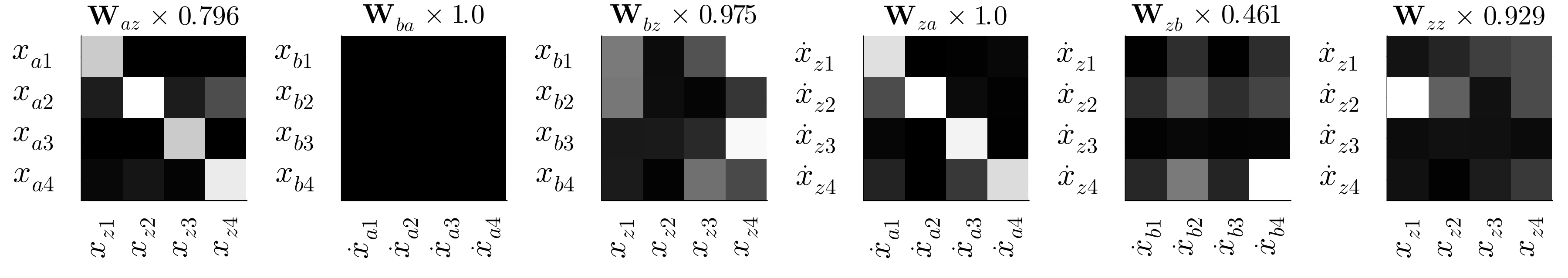
Figure 8: PFO: The matrices $\bm{W}_{az}$ and $\bm{W}_{za}$ are initialized with (noisy) identity, the remaining with (noisy) zeros. All matrix weights except $\bm{W}_{ba}$ are optimized together with the ANN parameters.

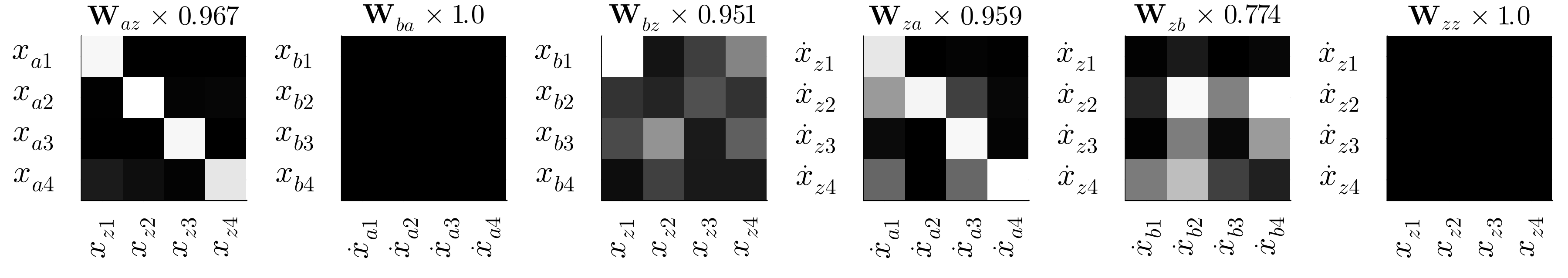
Figure 9: PO: The matrices $\bm{W}_{az}$ and $\bm{W}_{za}$ are initialized with (noisy) identity, the remaining with (noisy) zeros. All matrix weights except $\bm{W}_{ba}$ and $\bm{W}_{zz}$ are optimized together with the ANN parameters.

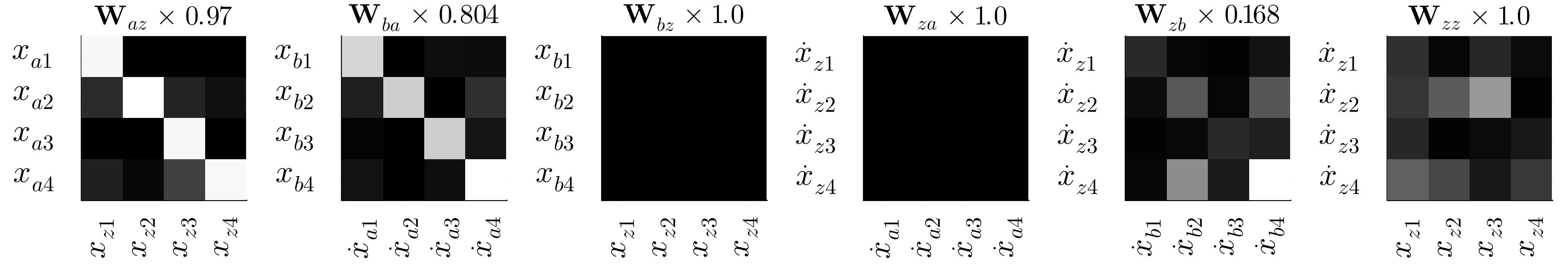
Figure 10: SFO: The matrices $\bm{W}_{az}$ and $\bm{W}_{ba}$ are initialized with (noisy) identity, the remaining with (noisy) zeros. All matrix weights except $\bm{W}_{bz}$ and $\bm{W}_{za}$ are optimized together with the ANN parameters.

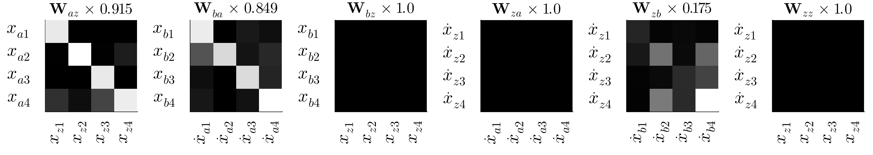
Figure 11: SO: The matrices $\bm{W}_{az}$ and $\bm{W}_{ba}$ are initialized with (noisy) identity, the remaining with (noisy) zeros. All matrix weights except $\bm{W}_{bz}$, $\bm{W}_{za}$ and $\bm{W}_{zz}$ are optimized together with the ANN parameters.

References

- [1] Albert Gu et al. “Combining Recurrent, Convolutional, and Continuous-time Models with Linear State Space Layers” In Advances in Neural Information Processing Systems 34 Curran Associates, Inc., 2021, pp. 572–585 URL: https://proceedings.neurips.cc/paper_files/paper/2021/file/05546b0e38ab9175cd905eebcc6ebb76-Paper.pdf
- [2] Yulia Rubanova, Ricky T.. Chen and David Duvenaud “Latent ODEs for Irregularly-Sampled Time Series”, 2019 arXiv:1907.03907 [cs.LG]
- [3] Ricky T.. Chen, Yulia Rubanova, Jesse Bettencourt and David K Duvenaud “Neural Ordinary Differential Equations” In Advances in Neural Information Processing Systems 31 Curran Associates, Inc., 2018 URL: https://proceedings.neurips.cc/paper_files/paper/2018/file/69386f6bb1dfed68692a24c8686939b9-Paper.pdf
- [4] Tobias Thummerer, Johannes Tintenherr and Lars Mikelsons “Hybrid modeling of the human cardiovascular system using NeuralFMUs” In Journal of Physics: Conference Series 2090.1 IOP Publishing, 2021, pp. 012155 DOI: 10.1088/1742-6596/2090/1/012155
- [5] Laura Rueden et al. “Combining Machine Learning and Simulation to a Hybrid Modelling Approach: Current and Future Directions” In Advances in Intelligent Data Analysis XVIII Cham: Springer International Publishing, 2020, pp. 548–560
- [6] Michael L. Thompson and Mark A. Kramer “Modeling chemical processes using prior knowledge and neural networks” In AIChE Journal 40.8, 1994, pp. 1328–1340 DOI: https://doi.org/10.1002/aic.690400806
- [7] B. Sohlberg and E.W. Jacobsen “GREY BOX MODELLING – BRANCHES AND EXPERIENCES” 17th IFAC World Congress In IFAC Proceedings Volumes 41.2, 2008, pp. 11415–11420 DOI: https://doi.org/10.3182/20080706-5-KR-1001.01934
- [8] Maja Rudolph, Stefan Kurz and Barbara Rakitsch “Hybrid modeling design patterns” In Journal of Mathematics in Industry 14.1 SpringerOpen, 2024, pp. 1–36
- [9] Fabian Jirasek and Hans Hasse “Combining Machine Learning with Physical Knowledge in Thermodynamic Modeling of Fluid Mixtures” In Annual Review of Chemical and Biomolecular Engineering 14.Volume 14, 2023 Annual Reviews, 2023, pp. 31–51 DOI: https://doi.org/10.1146/annurev-chembioeng-092220-025342
- [10] Leifur P. Leifsson, Hildur Saevarsdottir, Sven P. Sigurosson and Ari Vesteinsson “Grey-box modeling of an ocean vessel for operational optimization” EUROSIM 2007 In Simulation Modelling Practice and Theory 16.8, 2008, pp. 923–932 DOI: https://doi.org/10.1016/j.simpat.2008.03.006
- [11] Christopher Rackauckas et al. “Universal Differential Equations for Scientific Machine Learning”, 2021 arXiv:2001.04385 [cs.LG]
- [12] Tobias Thummerer, Johannes Stoljar and Lars Mikelsons “NeuralFMU: Presenting a Workflow for Integrating Hybrid NeuralODEs into Real-World Applications” In Electronics 11.19, 2022 DOI: 10.3390/electronics11193202
- [13] Robert Tarjan “Depth-First Search and Linear Graph Algorithms” In SIAM Journal on Computing 1.2, 1972, pp. 146–160 DOI: 10.1137/0201010
- [14] “Modelica” Accessed: 2024-05-23 URL: https://modelica.org/
- [15] Yingbo Ma et al. “ModelingToolkit: A Composable Graph Transformation System For Equation-Based Modeling”, 2021 arXiv:2103.05244 [cs.MS]
- [16] “Simulation and Model-Based Design” Accessed: 2024-05-23 URL: https://www.mathworks.com/products/simulink.html
- [17] Christopher Rackauckas and Qing Nie “DifferentialEquations.jl – A Performant and Feature-Rich Ecosystem for Solving Differential Equations in Julia” Exported from https://app.dimensions.ai on 2019/05/05 In The Journal of Open Research Software 5.1, 2017 DOI: 10.5334/jors.151
- [18] J. Revels, M. Lubin and T. Papamarkou “Forward-Mode Automatic Differentiation in Julia” In arXiv:1607.07892 [cs.MS], 2016 URL: https://arxiv.org/abs/1607.07892
- [19] Diederik P. Kingma and Jimmy Ba “Adam: A Method for Stochastic Optimization”, 2017 arXiv:1412.6980 [cs.LG]