Classical simulability of constant-depth linear-optical circuits with noise
Abstract
Noise is one of the main obstacles to realizing quantum devices that achieve a quantum computational advantage. A possible approach to minimize the noise effect is to employ shallow-depth quantum circuits since noise typically accumulates as circuit depth grows. In this work, we investigate the complexity of shallow-depth linear-optical circuits under the effects of photon loss and partial distinguishability. By establishing a correspondence between a linear-optical circuit and a bipartite graph, we show that the effects of photon loss and partial distinguishability are equivalent to removing the corresponding vertices. Using this correspondence and percolation theory, we prove that for constant-depth linear-optical circuits with single photons, there is a threshold of loss (noise) rate above which the linear-optical systems can be decomposed into smaller systems with high probability, which enables us to simulate the systems efficiently. Consequently, our result implies that even in shallow-depth circuits where noise is not accumulated enough, its effect may be sufficiently significant to make them efficiently simulable using classical algorithms due to its entanglement structure constituted by shallow-depth circuits.
I Introduction
Quantum optical platforms using photons are expected to play versatile roles in various quantum information processing tasks, such as quantum communication, quantum sensing, and quantum computing [1, 2, 3, 4, 5, 6]. Especially, quantum optical circuits using linear optics are more experimentally feasible and still have the potential to provide a quantum advantage for quantum computing; representative examples are boson sampling using single photons [7] or Knill-Laflamme-Milburn (KLM) protocol for universal quantum computation [8].
However, as in other experimental platforms, one of the main obstacles to implementing a large-scale quantum device to perform interesting quantum information processing is noise; especially, photon loss and partial distinguishability of photons in photonic devices are typically the most crucial noise sources [9, 10, 11, 12]. Through experimental realizations of intermediate-scale quantum devices using photons and thorough theoretical analysis of the effect of loss and noise, many recent results show that they can significantly reduce the computational power of the quantum devices [9, 10, 11, 12, 13, 14, 15, 16, 17, 18, 19, 20, 21]. Hence, there have been significant interests and efforts in reducing the effect of photon loss and partial distinguishability, such as developing quantum error correction codes [22, 23, 24, 25, 26].
Since the photon loss effect becomes more severe as circuit depth increases and eventually quantum circuits become easy to classically simulate in many cases [15, 16, 17, 19, 20, 21], for quantum computing, more specifically for demonstrating quantum computational advantage, another viable and promising path is to employ a shallow-depth quantum circuit to minimize the effect of photon loss. In fact, a worst-case constant-depth linear-optical circuit with single photons is proven to be hard to simulate exactly using classical computers unless the polynomial hierarchy (PH) collapses to a finite level [27]. Furthermore, there have been many attempts to prove the average-case hardness of approximate simulation of shallow-depth boson sampling circuits [28, 29, 30]. Since one of the main reasons to utilize shallow-depth circuits is to minimize the effect of noise and loss, a pertinent question that needs to be answered is whether shallow-depth circuits under the effect are hard to classically simulate or the effect again destroys the potential quantum advantage even from shallow-depth circuits.
To address this question, in this work, we analyze the computational complexity of constant-depth linear-optical circuits under photon loss and partial distinguishability and prove that when the input state is single photons, there exists a threshold of noise rates above which we can efficiently simulate the system using classical computers. The main idea is to associate a linear-optical circuit with a bipartite graph in such a way that the single photons correspond to one part of the vertices of the graph and the output modes correspond to the other part of the vertices of the graph and they are connected by edges if the single photons can propagate to the output modes through the linear-optical circuit. We then appropriately adapt a well-known result of percolation theory from the study of network [31, 32] to bipartite graphs, which states that if some of the vertices of a graph of bounded degree are randomly removed, the resultant graph is divided into disjoint logarithmically-small-size graphs with high probability. We then show that the effect of photon loss or partial distinguishability noise exactly corresponds to removing some of the vertices; thus, photon loss or partial distinguishability of photons effectively transforms constant-depth linear-optical circuits into logarithmically-small-size independent linear-optical circuits. Consequently, we can simulate the entire circuit by individually simulating each small-size linear-optical circuit. Our result suggests that while shallow-depth circuits are often believed to be less subject to loss and noise, it may not always be true because the entanglement constituted by shallow-depth circuits may be more easily destroyed by loss and noise. Finally, we numerically analyze the effect for various architectures and discuss a general condition for our result to hold.
II Linear-optical circuits with single photons
Let us consider -mode linear-optical circuits with single photons as an input state and arbitrary local measurement for the output state. Here, linear-optical circuits are composed of layers of beam splitters, which may be geometrically non-local. This setup is the basis of single-photon boson sampling [7] or the KLM protocol [8] for universal quantum computation. While the latter typically require sufficiently deep linear-optical circuits, in this work, we will mainly focus on much shallower depth circuits, more precisely, constant-depth circuits, which are expected to be less subject to loss and noise. We emphasize again that constant-depth boson sampling is proven to be hard to classically simulate unless the PH collapses to a finite level [27]; thus, shallow-depth linear-optical circuits may be sufficient for quantum computational advantage.
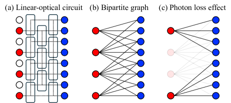
Let us associate a linear-optical circuit with a bipartite graph (see Fig. 1 (a)). To do that, let and be the set of input modes that are initialized by single photons and the set of output modes to which the input photons can propagate through the given linear-optical circuit, respectively. Thus, , and depends on the architecture and the circuit depth. We then introduce a bipartite graph constituted by and for vertices on the left and right, respectively, and edges between them. The edges of the bipartite graph are determined by the light cone of input photons through the linear-optical circuit; namely, if a photon from an input mode corresponding to can propagate to an output mode corresponding to , then the graph has an edge between the vertices, i.e., . Here, we define the size of a bipartite as the number of vertices on the left-hand side, i.e., .
Let us define to be the maximum degree of the bipartite graph , which is the maximum number of edges connected to a single vertex,
| (1) |
We note that when the depth of a linear-optical circuit is , the maximum degree of the associated bipartite graph is limited by because each beam splitter has two-mode input and output. Hence, when the circuit depth is a constant, i.e., , the number of output modes relevant to each single photon input is also for an arbitrary architecture. When the circuit is geometrically local, say -dimensional system, then each single photon can propagate up to . For example, when , and when , .
Using the introduced relation between linear-optical circuits and bipartite graphs and percolation theory, we investigate the complexity of simulating the linear-optical circuits under the effect of photon loss or partial distinguishability noise.
III Bipartite-Graph percolation
Percolation theory describes the behavior of graphs obtained by adding or deleting vertices or edges of graphs [31, 32]. Percolation theory has also been used in quantum information theory to study entanglement in quantum networks [33, 34, 35]. Also, very recently, it has been used to invent a classical algorithm for simulating constant-depth IQP circuits [36]. Using a similar technique, we will show that constant-depth linear-optical circuits with single photons are easy to classically simulate when the loss rate or the noise rate is sufficiently high. The key idea for this, together with the percolation lemma below, is that if a single photon is lost or becomes distinguishable from others, the system then essentially loses interference induced from the photon. This effect, from graph theoretically point of view, is to remove the vertex or to decouple the vertex from the graph for loss and distinguishability noise, respectively (see below for more details). To use this property, we adapt a result of percolation theory from Refs. [37, 38, 36] to bipartite graphs (see Appendix A for the proof):
Lemma 1.
Let be a bipartite graph of maximum degree . If we independently remove each with probability with and all edges incident to from , then the resultant bipartite graph is divided into bipartite graphs disconnected to each other and
| (2) |
Hence, when , with high probability , the largest graph size in is smaller than or equal to
| (3) |
From the physical point of view, the lemma implies that for a linear-optical circuit with maximum degree , losing portion of input states is so significant that the remaining system can be effectively described by many independent small-size systems.
It is worth emphasizing that the above lemma can be understood from a previous result [38, 36] by defining a graph based on the bipartite graph in such a way that the graph’s vertices are and two vertices have an edge if they are connected by a vertex in in the original bipartite graph. Physically, two input modes are connected if the photons from them can be outputted in the same output mode, i.e., they can interfere each other. Using the relation between the underlying bipartite and the new graph , we can easily see that the maximum degree of the graph is upper-bounded by .
IV Photon loss effect
Now, let us consider photon loss on input photons and observe the correspondence between photon loss and the removal of some vertices in the associated bipartite graph as in Lemma 1. When we prepare a single photon and then it is subject to a loss channel with loss rate , the single-photon state transforms as
| (4) |
Then, while there is no effect for the photon with probability , i.e., the vertex of the associated bipartite graph is kept, the vertex is removed from with probability . Consequently, when we prepare single photons and the single photons are subject to a loss channel with loss rate , the effect is to remove each vertex with probability independently, which is exactly the same procedure in Lemma 1 (see Fig. 1 for the illustration).
By taking advantage of this relation and Lemma 1, we propose a classical algorithm simulating linear-optical systems with single photon input when . First, we remove each vertex in with probability for the associated bipartite graph with a given linear-optical circuit with single photons. For the resultant graph, we identify components that are disconnected from each other. If the size of any connected component obtained from the first step is larger than , then we return to the first step. Otherwise, we now have with for all ’s. Since the number of photons for each connected component scales logarithmically, we can expect that it is easy to classically simulate. Here, is chosen to be the desired total variation distance (see below).
More specifically, to see how we simulate each system associated with as desired since the number of input photons in each is at most and the number of relevant output modes is at most , the associated Hilbert space’s dimension is upper-bounded by
| (5) |
where we used . Thus, when , which is the case for a constant depth circuit, the dimension is upper bounded by . Therefore, since writing down the output states and the relevant operators takes polynomial time in and for any local measurement, we can efficiently simulate the system. If the measurement is photon number detection, which corresponds to boson sampling [7], then one may simply use the Clifford-Clifford algorithm whose complexity is given by [39].
One may notice that if scales with the system size and the measurement is not on a photon number basis, the above counting gives us a superpolynomially increasing dimension in . For this case, to be more efficient, consider a number of single photons as an input and note that a linear-optical circuit transforms the creation operators of input modes as
| (6) |
where is the unitary matrix characterizing the linear-optical circuit with being the relevant number of modes, and we set a bipartite between output modes and . Then, the output state can be written as
| (7) |
Therefore, for any bipartition, the output state can be described by at most singular values, which means that there exists a matrix product state that can describe the state with bond dimension [40], which can be found by using time-evolution block decimation [41]. It is worth emphasizing that if the circuit is not linear-optical, the output bosonic operators may not be decomposed by a similar way and thus require more computational costs because it may contain an operator that is a product of two operators from each partition (e.g., ).
The remaining question is the algorithm’s error, which is caused by skipping the case where the connected component’s size is larger than . Recall that if we encounter the case where the maximum size of the connected components is larger than , then we restart the sampling. Then, the output probability of such an algorithm is given by
| (8) |
where is the conditional probability on the case where the maximum size of the connected components is smaller than or equal to ; hence, the true probability of the linear-optical circuit is written as
| (9) |
where is the case where the maximum size of the connected components is larger than . Then, the total variation distance between the suggested algorithm’s output probability and the true output probability can be shown to be smaller than (see Appendix C):
| (10) |
Finally, there is an overhead per sample due to the restart, but this is only , which is negligible. Thus, we obtain the following theorem:
Theorem 1.
For a given loss rate and a linear-optical circuit of an arbitrary architecture of maximum degree with single photon input, if , there exists a classical algorithm that can approximately simulate the corresponding lossy linear-optical circuits in within total variation distance .
Hence, for constant-depth linear-optical circuits, i.e., and thus , there is a threshold of loss rate above which it becomes classically easy to sample. Note that although we assumed the maximum degree to be to cover the worst case, the actual loss threshold depends on the architecture (see below for further discussion on this). It is worth emphasizing that the notion of approximate simulation is crucial because the exact classical simulation of constant-depth lossy linear-optical circuits is hard unless the PH collapses to a finite level. This can easily be shown by noting that postselecting no loss case of lossy boson sampling is equivalent to lossless boson sampling and constant-depth boson sampling with post-selection is post-BQP due to the measurement-based quantum computing [27]. Thus, if lossy constant-depth boson sampling can be exactly simulated using classical algorithms efficiently, [42], which contradicts the fact that is in the PH [43] assuming that the PH is infinite.
Here, we also consider cases where each layer of beam splitters has a transmission rate that is smaller than , and thus . Since for any architecture and loss channel with a loss rate commutes with beam splitters (see e.g., Refs. [15, 17]), we have the following corollary:
Corollary 1.
For a given transmission rate per layer and a linear-optical circuit of an arbitrary architecture of maximum degree with single photon input, if , there exists a classical algorithm that can approximately simulate the corresponding lossy linear-optical circuits in within total variation distance .
For this case, the presented matrix product state method is crucial because the depth may not be constant.
V Partial distinguishability noise
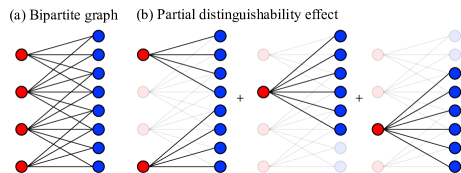
A similar observation can be used when input photons are partially distinguishable, which is another important noise model in optical systems [44, 14, 13, 45]. The underlying physical mechanism that causes photons to be partially distinguishable is other degrees of freedom of photons, such as polarization and temporal shapes. Consequently, when the other degrees of freedom do not match perfectly, the overlap of the wave functions of a pair of photons becomes less than 1 (see Ref. [44] for more discussion.). For simplicity, we assume that the overlap for any pairs of photons is uniform as .
Ref. [45] shows that such a model transforms an single-photon state to the following density matrix
| (11) |
where is the state whose elements are indistinguishable and others are distinguishable and . Then, the quantum state of the partially distinguishable single photons is equivalent to the mixture of an particle state, which is obtained by randomly selecting particles following a binomial distribution with success probability and setting them indistinguishable bosons and other fully distinguishable particles. Therefore, the remaining photons do not interfere with other particles. From the perspective of bipartite graphs and percolation, it corresponds to decoupling the corresponding vertices from the original bipartite graph as illustrated in Fig. 2. A difference from the photon loss effect is that whereas we remove the corresponding vertices for the case of photon loss, for the partial distinguishability effect, we remove the vertices and then construct bipartite graphs with each removed vertex. The percolation lemma still applies here because the resultant bipartite graphs still have the maximum size with high probability. Thus, the classical algorithm needs to be modified to simulate the systems corresponding to the new bipartite graphs with a single vertex on the left-hand side, and so we again have a similar theorem:
Theorem 2.
For a given partial distinguishability and a linear-optical circuit of an arbitrary architecture of maximum degree with single photon input, if , there exists a classical algorithm that can approximately simulate the corresponding lossy linear-optical circuits in within total variation distance .
VI Numerical result
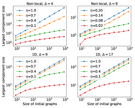
To clearly see the effect of photon loss or partial distinguishability on linear-optical systems, we numerically investigate the maximum size of components after randomly removing vertices from . We consider two different cases: linear-optical circuits (i) with non-local beam splitters and (ii) with 1D-local beam splitters. For simplicity of the numerical simulation, in the non-local case, for a given input photon number and a number of modes , we randomly generate , and, in the 1D case, we generate edges from each input mode to the closest output modes.
For a fixed and different loss rates, we increase the number of input modes and analyze the largest component size, i.e., , which is showcased in Fig. 3. First of all, it is clear that depending on the loss rates, the largest component size increases in distinct ways; when the loss rate is sufficiently low, it increases linearly, while the loss rate is high enough, it starts to increase logarithmically as expected by Lemma 1. We also emphasize that the transition point of the loss rate depends on the architecture. For instance, when , the transition occurs between and for 1D systems, whereas it occurs between and , which implies that the non-local structure is much more robust than the 1D structure. Therefore, while Lemma 1 presents the worst-case threshold, the actual threshold may depend on the details of the architecture, such as the geometry of the architecture (e.g., non-local beam splitters or geometrically local beam splitters.) and how many output modes are relevant.
VII Discussion on more general cases
We now discuss the possibility of generalizing the above results to more general setups. First of all, for photon-loss cases, it is not hard to see that even if we replace single photons with general Fock states , a similar theorem holds. This is because a Fock state with photon number transforms under photon loss as
| (12) | ||||
| (13) |
Therefore, we can follow the same procedure as single-photon cases. A difference is that to see the percolation effect, now we sample from a binomial distribution with failure probability , which corresponds to vacuum input and thus the associated vertex is removed from the bipartite graph. Consequently, the percolation threshold becomes
| (14) |
For this case, since each input mode has at most photons, the associated Hilbert space’s dimension for is at most
| (15) |
Similarly, for other more general input states than Fock states, if the largest photon number of each input state for each mode is bounded by a constant, then the Hilbert space’s dimension is at most polynomial in ; more generally, as long as the largest total number of photons is bounded by a linear function of , the Hilbert space’s dimension is still upper bounded by . For larger depth , we again need to use the matrix produce state method (see Appendix B for more details).
Hence, one may see that a sufficient condition for the percolation result to apply is that the lossy input state is written as
| (16) |
where , , , and can be written in the Fock basis with at most a constant photon number. As the Fock state example implies, the threshold value depends on how the input state transforms under a loss channel. Thus, an analytic way to compute the threshold value for arbitrary input states has to be further studied. Also, we emphasize that the assumption that the circuit is linear-optical is important because otherwise, we may be able to apply an operation that generates photons in the middle of the circuit, such as a squeezing operation, after the loss channel on the input.
VIII Discussion
In this work, we showed that a threshold of loss or noise rate exists above which classical computers can efficiently simulate constant-depth linear-optical circuits with certain input states. Our result implies that shallow-depth circuits may also be vulnerable to loss and noise because the entanglement in the system constructed by shallow-depth circuits may be more easily annihilated by noise.
An interesting future work is to find a general condition for the input states under which the percolation result gives the easiness result. Whereas Fock states’ threshold is easily found, it is not immediately clear to analytically find the threshold of more general quantum states, such as Gaussian states. Also, while our results hold for arbitrary architecture as long as the depth is constant, the depth limit might be pushed further depending on the details of the architecture, such as the geometry of the circuits and the input state configuration [46, 47]. Conversely, investigating the possibility of the hardness of constant-depth boson sampling with a loss rate below the threshold is another interesting future work enabling us to demonstrate quantum advantage even under practical loss and noise effects. Finally, we can easily see that the percolation lemma immediately applies for a continuous-variable erasure channel considered in Refs. [48, 49, 50]. Thus, we may be able to apply a similar technique to other noise models, such as more general Gaussian noise [51].
Acknowledgements.
We thank Byeongseon Go and Senrui Chen for interesting and fruitful discussions. This research was supported by Quantum Technology R&D Leading Program (Quantum Computing) (RS-2024-00431768) through the National Research Foundation of Korea (NRF) funded by the Korean government (Ministry of Science and ICT (MSIT))References
- Duan et al. [2001] L.-M. Duan, M. D. Lukin, J. I. Cirac, and P. Zoller, Long-distance quantum communication with atomic ensembles and linear optics, Nature 414, 413 (2001).
- Kok et al. [2007] P. Kok, W. J. Munro, K. Nemoto, T. C. Ralph, J. P. Dowling, and G. J. Milburn, Linear optical quantum computing with photonic qubits, Reviews of modern physics 79, 135 (2007).
- Sangouard et al. [2011] N. Sangouard, C. Simon, H. De Riedmatten, and N. Gisin, Quantum repeaters based on atomic ensembles and linear optics, Reviews of Modern Physics 83, 33 (2011).
- Pirandola et al. [2018] S. Pirandola, B. R. Bardhan, T. Gehring, C. Weedbrook, and S. Lloyd, Advances in photonic quantum sensing, Nature Photonics 12, 724 (2018).
- Slussarenko and Pryde [2019] S. Slussarenko and G. J. Pryde, Photonic quantum information processing: A concise review, Applied Physics Reviews 6 (2019).
- Bourassa et al. [2021] J. E. Bourassa, R. N. Alexander, M. Vasmer, A. Patil, I. Tzitrin, T. Matsuura, D. Su, B. Q. Baragiola, S. Guha, G. Dauphinais, et al., Blueprint for a scalable photonic fault-tolerant quantum computer, Quantum 5, 392 (2021).
- Aaronson and Arkhipov [2011] S. Aaronson and A. Arkhipov, The computational complexity of linear optics, in Proceedings of the forty-third annual ACM symposium on Theory of computing (2011) pp. 333–342.
- Knill et al. [2001] E. Knill, R. Laflamme, and G. J. Milburn, A scheme for efficient quantum computation with linear optics, nature 409, 46 (2001).
- Zhong et al. [2020] H.-S. Zhong, H. Wang, Y.-H. Deng, M.-C. Chen, L.-C. Peng, Y.-H. Luo, J. Qin, D. Wu, X. Ding, Y. Hu, et al., Quantum computational advantage using photons, Science 370, 1460 (2020).
- Zhong et al. [2021] H.-S. Zhong, Y.-H. Deng, J. Qin, H. Wang, M.-C. Chen, L.-C. Peng, Y.-H. Luo, D. Wu, S.-Q. Gong, H. Su, et al., Phase-programmable Gaussian boson sampling using stimulated squeezed light, Physical review letters 127, 180502 (2021).
- Madsen et al. [2022] L. S. Madsen, F. Laudenbach, M. F. Askarani, F. Rortais, T. Vincent, J. F. Bulmer, F. M. Miatto, L. Neuhaus, L. G. Helt, M. J. Collins, et al., Quantum computational advantage with a programmable photonic processor, Nature 606, 75 (2022).
- Deng et al. [2023] Y.-H. Deng, Y.-C. Gu, H.-L. Liu, S.-Q. Gong, H. Su, Z.-J. Zhang, H.-Y. Tang, M.-H. Jia, J.-M. Xu, M.-C. Chen, et al., Gaussian boson sampling with pseudo-photon-number-resolving detectors and quantum computational advantage, Physical review letters 131, 150601 (2023).
- Renema et al. [2018a] J. Renema, V. Shchesnovich, and R. Garcia-Patron, Classical simulability of noisy boson sampling, arXiv preprint arXiv:1809.01953 (2018a).
- Renema et al. [2018b] J. J. Renema, A. Menssen, W. R. Clements, G. Triginer, W. S. Kolthammer, and I. A. Walmsley, Efficient classical algorithm for boson sampling with partially distinguishable photons, Physical review letters 120, 220502 (2018b).
- García-Patrón et al. [2019] R. García-Patrón, J. J. Renema, and V. Shchesnovich, Simulating boson sampling in lossy architectures, Quantum 3, 169 (2019).
- Qi et al. [2020] H. Qi, D. J. Brod, N. Quesada, and R. García-Patrón, Regimes of classical simulability for noisy gaussian boson sampling, Physical review letters 124, 100502 (2020).
- Oh et al. [2021] C. Oh, K. Noh, B. Fefferman, and L. Jiang, Classical simulation of lossy boson sampling using matrix product operators, Physical Review A 104, 022407 (2021).
- Shi and Byrnes [2022] J. Shi and T. Byrnes, Effect of partial distinguishability on quantum supremacy in gaussian boson sampling, npj Quantum Information 8, 54 (2022).
- Oh et al. [2023a] C. Oh, L. Jiang, and B. Fefferman, On classical simulation algorithms for noisy boson sampling, arXiv preprint arXiv:2301.11532 (2023a).
- Liu et al. [2023] M. Liu, C. Oh, J. Liu, L. Jiang, and Y. Alexeev, Simulating lossy gaussian boson sampling with matrix-product operators, Physical Review A 108, 052604 (2023).
- Oh et al. [2023b] C. Oh, M. Liu, Y. Alexeev, B. Fefferman, and L. Jiang, Tensor network algorithm for simulating experimental gaussian boson sampling, arXiv preprint arXiv:2306.03709 (2023b).
- Michael et al. [2016] M. H. Michael, M. Silveri, R. Brierley, V. V. Albert, J. Salmilehto, L. Jiang, and S. M. Girvin, New class of quantum error-correcting codes for a bosonic mode, Physical Review X 6, 031006 (2016).
- Chamberland et al. [2022] C. Chamberland, K. Noh, P. Arrangoiz-Arriola, E. T. Campbell, C. T. Hann, J. Iverson, H. Putterman, T. C. Bohdanowicz, S. T. Flammia, A. Keller, et al., Building a fault-tolerant quantum computer using concatenated cat codes, PRX Quantum 3, 010329 (2022).
- Marshall [2022] J. Marshall, Distillation of indistinguishable photons, Physical Review Letters 129, 213601 (2022).
- Sivak et al. [2023] V. Sivak, A. Eickbusch, B. Royer, S. Singh, I. Tsioutsios, S. Ganjam, A. Miano, B. Brock, A. Ding, L. Frunzio, et al., Real-time quantum error correction beyond break-even, Nature 616, 50 (2023).
- Faurby et al. [2024] C. F. Faurby, L. Carosini, H. Cao, P. I. Sund, L. M. Hansen, F. Giorgino, A. B. Villadsen, S. N. Hoven, P. Lodahl, S. Paesani, et al., Purifying photon indistinguishability through quantum interference, arXiv preprint arXiv:2403.12866 (2024).
- Brod [2015] D. J. Brod, Complexity of simulating constant-depth bosonsampling, Physical Review A 91, 042316 (2015).
- van der Meer et al. [2021] R. van der Meer, S. Huber, P. Pinkse, R. García-Patrón, and J. Renema, Boson sampling in low-depth optical systems, arXiv preprint arXiv:2110.05099 (2021).
- Go et al. [2024a] B. Go, C. Oh, L. Jiang, and H. Jeong, Exploring shallow-depth boson sampling: Toward a scalable quantum advantage, Physical Review A 109, 052613 (2024a).
- Go et al. [2024b] B. Go, C. Oh, and H. Jeong, On computational complexity and average-case hardness of shallow-depth boson sampling, arXiv preprint arXiv:2405.01786 (2024b).
- Shante and Kirkpatrick [1971] V. K. Shante and S. Kirkpatrick, An introduction to percolation theory, Advances in Physics 20, 325 (1971).
- Sahimi [1994] M. Sahimi, Applications of percolation theory (CRC Press, 1994).
- Acín et al. [2007] A. Acín, J. I. Cirac, and M. Lewenstein, Entanglement percolation in quantum networks, Nature Physics 3, 256 (2007).
- Cuquet and Calsamiglia [2009] M. Cuquet and J. Calsamiglia, Entanglement percolation in quantum complex networks, Physical review letters 103, 240503 (2009).
- Pant et al. [2019] M. Pant, D. Towsley, D. Englund, and S. Guha, Percolation thresholds for photonic quantum computing, Nature communications 10, 1070 (2019).
- Rajakumar et al. [2024] J. Rajakumar, J. D. Watson, and Y.-K. Liu, Polynomial-time classical simulation of noisy iqp circuits with constant depth, arXiv preprint arXiv:2403.14607 (2024).
- Grimmett and Grimmett [1999] G. Grimmett and G. Grimmett, Some basic techniques, in Percolation (Springer, 1999) pp. 32–52.
- Krivelevich [2014] M. Krivelevich, The phase transition in site percolation on pseudo-random graphs, arXiv preprint arXiv:1404.5731 (2014).
- Clifford and Clifford [2018] P. Clifford and R. Clifford, The classical complexity of boson sampling, in Proceedings of the Twenty-Ninth Annual ACM-SIAM Symposium on Discrete Algorithms (SIAM, 2018) pp. 146–155.
- Vidal [2003] G. Vidal, Efficient classical simulation of slightly entangled quantum computations, Phys. Rev. Lett. 91, 147902 (2003).
- Schollwöck [2011] U. Schollwöck, The density-matrix renormalization group in the age of matrix product states, Annals of physics 326, 96 (2011).
- Aaronson [2005] S. Aaronson, Quantum computing, postselection, and probabilistic polynomial-time, Proceedings of the Royal Society A: Mathematical, Physical and Engineering Sciences 461, 3473 (2005).
- Han et al. [1997] Y. Han, L. A. Hemaspaandra, and T. Thierauf, Threshold computation and cryptographic security, SIAM Journal on Computing 26, 59 (1997).
- Tichy [2015] M. C. Tichy, Sampling of partially distinguishable bosons and the relation to the multidimensional permanent, Physical Review A 91, 022316 (2015).
- Moylett et al. [2019] A. E. Moylett, R. García-Patrón, J. J. Renema, and P. S. Turner, Classically simulating near-term partially-distinguishable and lossy boson sampling, Quantum Science and Technology 5, 015001 (2019).
- Deshpande et al. [2018] A. Deshpande, B. Fefferman, M. C. Tran, M. Foss-Feig, and A. V. Gorshkov, Dynamical phase transitions in sampling complexity, Physical review letters 121, 030501 (2018).
- Oh et al. [2022] C. Oh, Y. Lim, B. Fefferman, and L. Jiang, Classical simulation of boson sampling based on graph structure, Physical Review Letters 128, 190501 (2022).
- Wittmann et al. [2008] C. Wittmann, D. Elser, U. L. Andersen, R. Filip, P. Marek, and G. Leuchs, Quantum filtering of optical coherent states, Physical Review A 78, 032315 (2008).
- Lassen et al. [2010] M. Lassen, M. Sabuncu, A. Huck, J. Niset, G. Leuchs, N. J. Cerf, and U. L. Andersen, Quantum optical coherence can survive photon losses using a continuous-variable quantum erasure-correcting code, Nature Photonics 4, 700 (2010).
- Zhong et al. [2023] C. Zhong, C. Oh, and L. Jiang, Information transmission with continuous variable quantum erasure channels, Quantum 7, 939 (2023).
- Serafini [2017] A. Serafini, Quantum continuous variables: a primer of theoretical methods (CRC press, 2017).
Appendix A Proof of Lemma 1
In this Appendix, we provide the proof of Lemma 1 in the main text. The proof is based on Refs. [37, 38, 36] and is adapted to bipartite-graph cases.
Proof.
Suppose we have an by bipartite graph with maximum degree and then remove some vertices on the left-hand side with probability and edges connected to them.
We present an algorithm that constructs a random graph as described in the lemma. Denote the set of the vertices on the left-hand side as and on the left-hand side as . We initialize this to be the empty graph. Then, we construct by querying the vertices on . A query to vertex succeeds with probability , in which case the vertex is added to . When , the algorithm initializes by querying all unqueried vertices in until the first successful query. When , the algorithm queries all unqueried vertices in , where is a subset of which is connected by through by one step. The size of is upper-bounded by . Whenever the algorithm runs out of unqueried vertices, it adds , the vertices in connected to , and corresponding edges to and resets and continues. The algorithm finishes when there are no more unqueried vertices in . Note that when the algorithm adds and its corresponding vertices in and edges to , the added graph is always disconnected to the one in every step, which results in the set of disjoint components , where is the number of steps.
If there is a component of size or higher, must have reached at some point. At this point, suppose the most recent vertex added to is labeled . To reach this point, we could have made at most queries with exactly being successful. Hence, the probability of forming a of size or higher is upper bounded as
| (17) |
Here, means the probability of obtaining more than successes from binomial sampling out of trials with success probability . Using the Chernoff bound with mean ,
| (18) |
with setting ,
| (19) | ||||
| (20) | ||||
| (21) |
By applying the union bound,
| (22) | ||||
| (23) |
∎
Appendix B Matrix product state for more general states than single photons
In this Appendix, we show that any linear-optical circuits with input states that have a constant maximum photon number can be simulated by matrix product state with bond dimension at most ; thus, the computational cost is exponential in with a constant .
Let us consider a linear-optical circuit , which transforms the creation operators of input modes into the creation operators of output modes as
| (24) |
where is an unitary matrix characterizing the linear-optical circuit . When we prepare input states with maximum photon number ,
| (25) |
the total input state transforms as
| (26) | ||||
| (27) | ||||
| (28) |
Thus, the output state can be written as the linear combination of at most vectors that are a product of a vector in u and a vector in d. Therefore, as long as is constant, the output state requires at most an exponential number of singular values; hence, the matrix product state method can simulate the system.
Appendix C Upper bound of total variation distance
In this Appendix, we derive the upper bound of the approximation error caused by skipping the case where the connected component’s size is larger than . Recall that the output probability of such an algorithm is given by
| (29) |
where is the true conditional probability of the case where the maximum size of the connected components is smaller than or equal to ; hence, the true probability is written as
| (30) |
where is the case where the maximum size of the connected components is larger than . Then, the total variation distance between the suggested algorithm’s output probability and the true output probability can be shown to be smaller than :
| (31) | |||
| (32) | |||
| (33) | |||
| (34) | |||
| (35) |