Daniel Sank
Mostafa Khezri
Sergei Isakov
Juan Atalaya
Google Quantum AI, Goleta, CA
Abstract
The rotating wave approximation (RWA) is ubiquitous in the analysis of driven and coupled resonators.
However, the limitations of the RWA seem to be poorly understood and in some cases the RWA disposes of essential physics.
We investigate the RWA in the context of electrical resonant circuits.
Using a classical Hamiltonian approach, we find that by balancing electrical and magnetic components of the resonator drive or resonator-resonator coupling, the RWA can be made exact.
This type of balance, in which the RWA is exact, has applications in superconducting qubits where it suppresses nutation normally associated with strong Rabi driving.
In the context of dispersive readout, balancing the qubit-resonator coupling changes the qubit leakage induced by the resonator drive (MIST), but does not remove it in the case of the transmon qubit.
\levelstay
Introduction
Analysis of driven and coupled resonators is pervasive throughout physics and engineering, and the case of electrical resonators has attracted particularly strong attention due to the success of superconducting circuits in quantum computing [1, 2].
Theoretical analyses almost universally use the rotating wave approximation (RWA) wherein fast terms in the system’s equations of motion are neglected.
The RWA simplifies the equations of motion for driven and coupled resonators, and for coupled resonators it greatly simplifies expressions for the normal mode frequencies.
Nevertheless, the validity of the RWA seems to be poorly understood.
The RWA is invoked in the coupled mode theory at the foundation of design of parametrically driven and non-reciprocal devices, used for example in Refs. [3, 4, 5].
Each of these references ultimately refers to Ref. [6] which justifies the RWA entirely by the fact that the RWA leads to a good approximation for the normal mode frequencies of coupled resonators.
But how well does the RWA capture the dynamics of real devices?
The RWA is known to fail in the case of superconducting qubit readout, where a weakly anharmonic resonator (transmon qubit) is coupled to a harmonic resonator.
In that case, higher order transitions between quantum levels in the coupled qubit-resonator system were found to spoil the readout process [7] even though those transitions are absent in the traditional RWA analysis [8, 9, 10, 11].
The RWA has also come under some scrutiny recently [12] as lowering the frequency of superconducting qubits has been pursued as a way to increase their energy decay lifetimes.
As the qubit frequency approaches the frequency of driven Rabi oscillations used for logic gates, the assumptions of the RWA are violated and it cannot be expected to be accurate.
With these examples in mind, a natural question is whether we can engineer the driving or coupling of electromagnetic resonators to actually remove the fast terms at the hardware level, i.e. to make the RWA exact.
If we can do this, then not only would the devices be easier to analyze, but also the deleterious processes found in Ref. [7] might be suppressed.
In this paper, we show that by balancing the electric and magnetic aspects of driven and coupled resonators, we can remove the fast oscillating terms and make the RWA exact.
The paper is organized as follows.
Section Balanced Coupling in Electromagnetic Circuits provides mathematical analysis of a driven resonator, showing how proper balance between the amplitudes and phases of simultaneous capacitive (electric) and inductive (magnetic) drives makes the RWA exact.
Section 3 analyzes two coupled resonators, showing that the RWA can be made exact if the coupling uses a balance of capacitive and inductive parts.
Application to readout of superconducting qubits is discussed.
Section 6 shows that the RWA appears in the analysis of coupled transmission lines, and that the design of a directional coupler is equivalent to making the RWA exact.
Finally, section 7 offers conclusions.
\levelstay
Balanced Drive
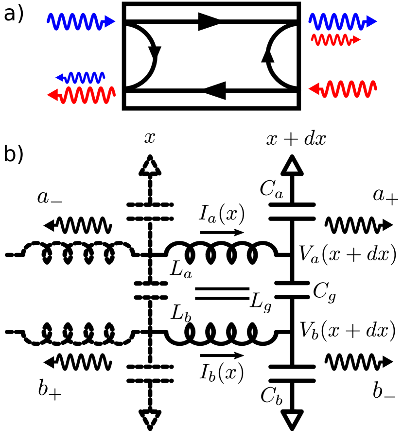
Figure 1: Capacitively and inductively driven resonator.
An LC resonator driven both capacitively and inductively is shown in Figure 1.
Kirchhoff’s laws for this circuit are
(1)
(2)
Going through the usual process of guessing the Lagrangian and then converting to the Hamiltonian, we find
(3)
where .
Details are given in Appendix A.
The symmetry between the flux and charge terms, and between the voltage and current drive terms, is brought out by defining the impedance , flux and charge scales and 111 and are the flux and charge zero point fluctuations in the ground state of the quantum LC resonator., and dimensionless variables and .
Using these variables, the Hamiltonian is
(4)
where
and
renormalize the drive magnitudes.
Here and are arbitrary constants with dimensions of voltage and current introduced so that and are dimensionless.
The equations of motion are
(5)
and in the absence of the drive the solutions are and where .
This motion is analogous to a spin precessing in space as described in Appendix 7, and just as is done in analysis of a driven precessing spin, it’s convenient here to use a coordinate frame rotating with the intrinsic motion.
Passage to the rotating coordinate frame is easier with the mode variables and defined by
With these variables, the Hamiltonian is
(6)
where .
The equations of motion are
(7)
and in the absence of the drive the solution is .
We switch to the rotating frame by defining and the Hamiltonian in the rotating frame is
(8)
In typical experiments either the electric or the magnetic part of the drive is present, but not both.
For example, the electric part may be absent, i.e. , and the magnetic part may be sinusoidal, .
In this case
(9)
Superconducting quantum devices have resonance frequencies in the range and control pulses are typically applied close to resonance, so while the slow terms may have frequencies , the fast terms oscillate at .
The RWA drops the fast-oscillating terms, typically with the justification that, in the weak driving limit where , such fast terms cannot significantly affect the dynamics.
It should be noted, however, that recent interest in lowering the resonance frequency of quantum devices to below while maintaining strong driving [14, 15, 16, 17] pushes the limits of the weak driving assumption and so non-RWA effects may come into play.
However, if both the electric and magnetic parts of the drive are included with equal magnitude and one quarter cycle phase offset, i.e.
(10)
then and the drive Hamiltonian is
(11)
where the fast terms have vanished exactly.
Condition (10) says that for the RWA to be exact, the electric and magnetic drive strengths must be equal, and the charge drive must lag the flux drive by one quarter of a cycle ( radians), a condition we call “balanced drive”.
This is the first main result of the paper: true rotating drive fields can be constructed in electromagnetic resonators by balancing the strengths of the electric and magnetic parts of the drive.
The result applies to any one dimensional system so long as the drive can be coupled to both the position and its conjugate momentum, but the electromagnetic case is particularly interesting because simultaneous capacitive and inductive drive coupling is routine in experiments.
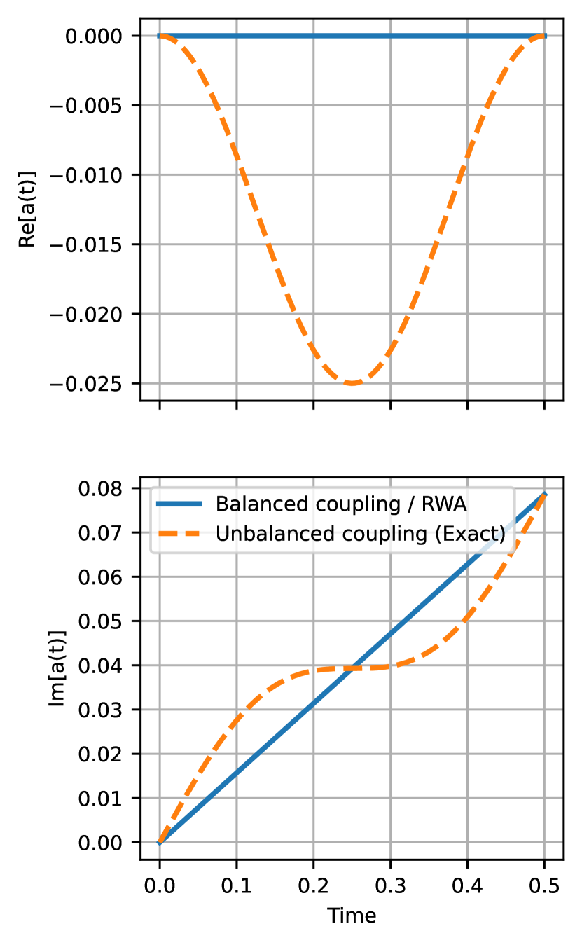
For an unbalanced purely inductive drive turning on at , i.e. for and for , the time evolution of the resonator amplitude is
(12)
Invoking the RWA or using balanced drive with drops the second term.
The dynamics with and are shown in Fig. 2.
When the drive is balanced or when we make the RWA with an unbalanced drive, the oscillator’s imaginary part increases linearly while the real part remains zero (solid blue curve).
On the other hand, when the drive is not balanced and we do not invoke the RWA, the real and imaginary parts both suffer an oscillation with period (broken orange curve).
Figure 2: Dynamics of a driven harmonic resonator. The blue solid curve corresponds to balanced drive or invoking the RWA with unbalanced drive. The orange broken curve shows the exact solution with unbalanced drive, i.e. Eq. (12).
Balanced drive may allow strong driving of low frequency superconducting circuits such as fluxonium, or even transmons operated at low frequency to enhance their energy decay lifetimes .
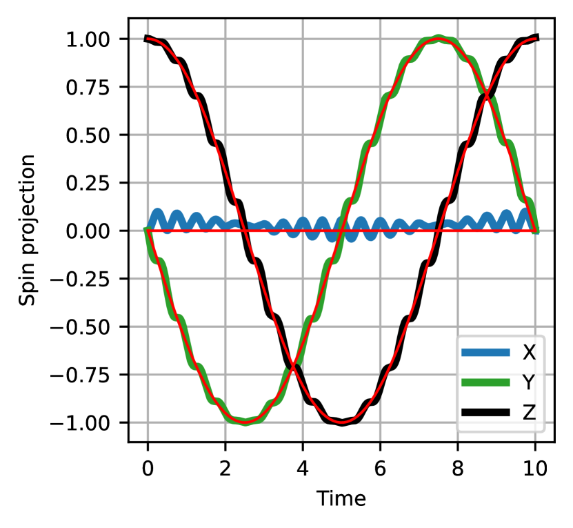
The Hamiltonian for the driven two level system may be obtained from Eq. (8) through the replacements and .
Figure 3 shows the expectation values of the Pauli operators for a two level system driven on resonance with and .
In the exact solution with unbalanced drive (blue, green, black) the trajectory exhibits nutation, i.e. each component suffers a fast oscillation on top of the usual rotation around the Bloch sphere.
On the other hand, with the balanced drive (red) the nutation is removed and the trajectories are smooth.
These predictions were recently verified in an experiment with fluxonium, where the balanced drive was shown to remove nutation in Rabi oscillations [18].
Figure 3: Trajectory of a two level system driven on resonance. The blue, green, and black curves show exact solutions of the , , and projections of the system in the case of unbalanced drive. The thin red curves show the trajectories when invoking the RWA or when using balanced drive.
\levelstay
Two-mode balanced coupling
Figure 4: Two resonators coupled capacitively and inductively.
We now consider the case of two coupled LC resonators as shown in Figure 4.
Kirchhoff’s laws for this circuit give us four equations
(13)
Note that the sense of the mutual inductance is defined such that a positive value of induces a positive contribution to , and vice versa.
Going through the usual process of finding the Lagrangian and then converting to the Hamiltonian, we find the Hamiltonian
(14)
where we defined
(15)
where , , , and are normalized frequency, impedance, capacitance, and inductance of the coupled resonators.
Details are given in Appendix B.
Hamilton’s equations of motion can now be expressed in matrix form
There are two aspects to the coupling.
The coupling connects to and to , i.e. it acts within the upper and lower diagonal 2x2 sub-blocks of .
On the other hand, the coupling couples to and to as it lies on the anti-diagonal of .
The structure of and the roles of the two aspects of coupling can be clearly seen by writing in algebraic form as
(16)
where and .
\leveldown
Rotating wave approximation
In the rotating frame, defined by and , the equation of motion for is
(17)
The time dependence of the first term on the right hand side is much slower than the second term, and just as in the case of the driven resonator, the fast term is dropped under the RWA.
Dropping the fast terms in the equations of motion is equivalent to dropping the and terms of the coupling Hamiltonian, i.e. dropping the terms of proportional to (the antidiagonal).
Therefore, if we engineer the coupling such that is identically zero, then the RWA will be exact.
The condition means , i.e. the capacitive and inductive coupling must be of equal magnitude but opposite sign, which we call “balanced coupling”.
Balanced coupling can also be expressed as the condition , i.e. the coupling impedance is equal to minus the geometric mean of the impedances of the two resonators.
Recall that a negative value for means that the mutual inductance must be arranged so that a positive value of produces a negative contribution to .
If the capacitive coupling is positive, then balanced coupling requires the mutual inductance to be negative.
The antidiagonal of corresponds to the term in ’s algebraic representation.
In the matrix, we see that dropping these terms decouples the clockwise and counterclockwise rotating modes, so the RWA drops the part of the dynamics coupling the clockwise-rotating modes to the counterclockwise-rotating modes.
Appendix B compares the full eigenvalues of with the eigenvalues of under the RWA.
\levelstay
Readout
Balanced coupling may have applications in readout of superconducting qubits.
Superconducting qubits are typically measured via dispersive coupling to a harmonic resonator [8, 19, 20, 21].
Unfortunately, introducing even modest levels of energy into the resonator during the readout activates resonances in the coupled qubit-resonator system that kick the qubit into noncomputational states high above the transmon potential [7, 22, 23, 24, 25].
This effect, called measurement-induced state transitions (MIST), is poisonous to quantum error correction [26] as occupation of noncomputational states leads to correlated errors and is difficult to reset.
MIST is a major challenge for quantum computing with superconducting qubits.
Critically, in the usual case where the resonator frequency is larger than the qubit frequency, the resonances responsible for MIST are mediated precisely by the excitation nonpreserving “non-RWA” terms in the coupling Hamiltonian, i.e. the terms that are neglected in the RWA [11, 7].
Therefore, in a circuit with balanced coupling between the qubit and resonator, MIST may be partially suppressed.
On the other hand, we should not expect perfect suppression because the preceding analysis is for two coupled harmonic resonators while qubits are by definition anharmonic.
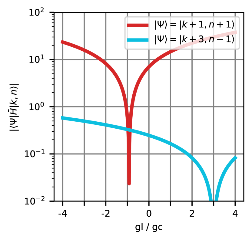
To see whether or not MIST can be removed with balanced coupling, we study the matrix elements of the transmon-resonator coupling Hamiltonian.
A perturbative expansion of the coupling is given in Appendix 8.
Using that expansion, we calculate the matrix elements connecting the initial state with final states and , each having two excitations more than the initial state and therefore requiring non-RWA coupling terms.
These particular final states are of interest because they may serve as intermediate virtual states in one of the two MIST transitions identified in Ref. [7].
Results are shown in Fig. 5.
Interestingly, the matrix element for vanishes when , close to the balanced coupling condition discussed above for coupled harmonic resonators.
The matrix element for vanishes for .
However, there is no ratio for which both matrix elements vanish simultaneously.
We emphasize that these ratios are calculated using a perturbative treatment.
Figure 5:
Perturbative calculation of two of the matrix elements taking the system from state to and .
The curves here are for the case , , , and .
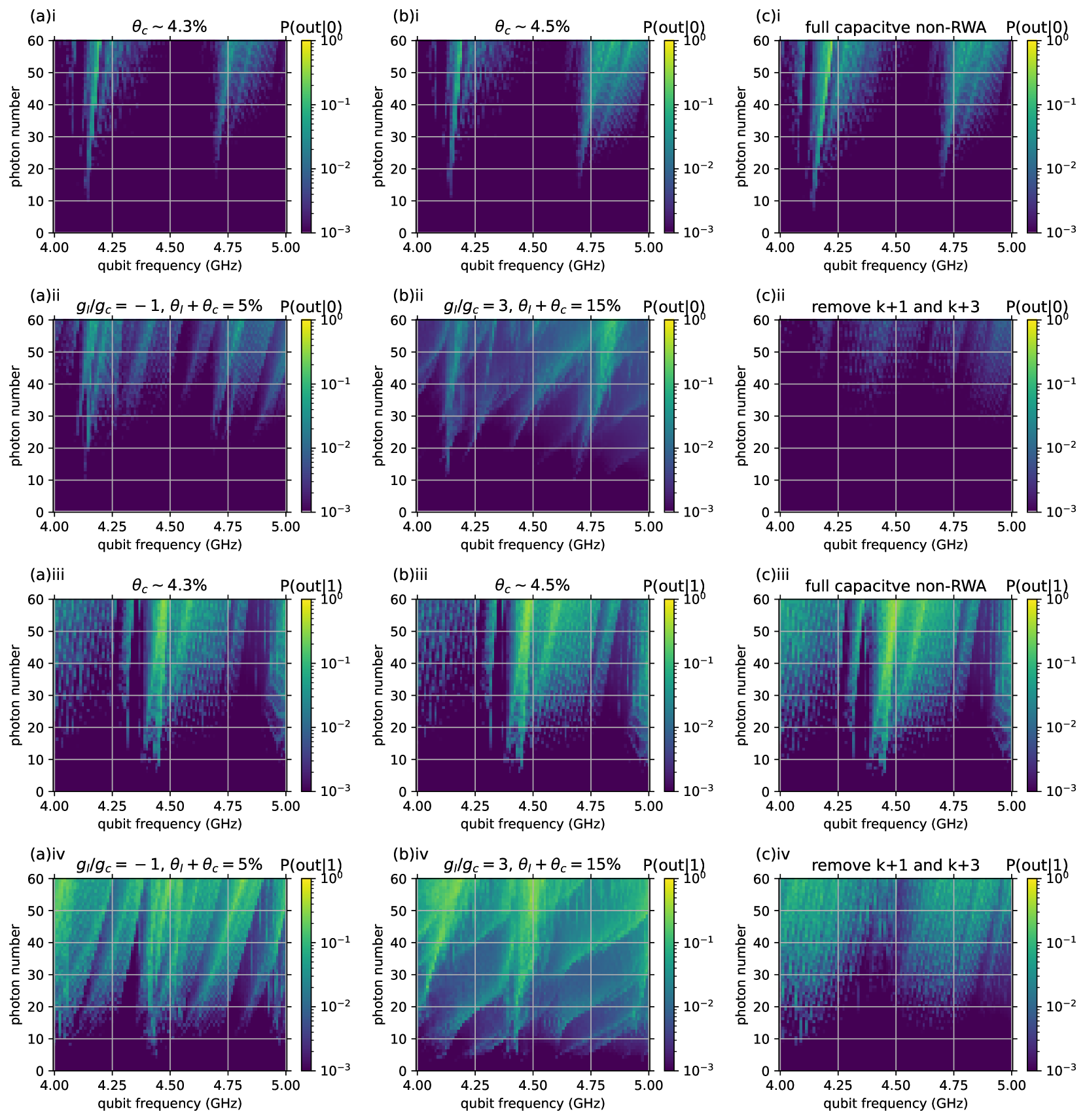
We numerically simulate the semiclassical model described in Ref. [22] but here tailored to account for non-RWA interactions.
The simulation proceeds in two steps.
We first simulate the driven resonator under the influence of a classical drive, where the resonator forms a coherent state.
We then treat the resonator field as a classical drive applied to the qubit [22, 24].
The qubit-resonator coupling is with coupling efficiency .
The resonator frequency is and the resonator linewidth is .
The qubit frequency is set to a value between and , with transmon charging energy of .
We perform the simulation once with balanced coupling and a fixed total coupling efficiency and then again with purely capacitive coupling, but we adjust the latter coupling to achieve the same dispersive shift as in the balanced case at each qubit frequency.
Keeping the same dispersive shift ensures a meaningful comparison of the readout performance at each frequency.
We also repeat the simulation for a set of 20 equally spaced transmon gate offset charges in the range and average the results.
Figure 6:
Simulations of MIST for the coupled qubit-resonator with and without balanced coupling, for different ratios.
First two rows show the result for qubit prepared in , and the second two rows for qubit prepared in .
(a) Simulations for balanced coupling with , with total balanced coupling efficiency of 0.05.
Panels i and iii show the capacitive case, and panel ii and iv show the balanced case.
(b) Simulations for balanced coupling with , with total balanced coupling efficiency of 0.15.
The large coupling efficiency is chosen to roughly yield the same dispersive shift as in the case of panels (a)i-iv.
Panels i and iii show the capacitive case, and panel ii and iv show the balanced case.
(c) Simulations for capacitive only case with capacitive coupling efficiency of 0.05.
Panels i and iii show the case were we retain all the non-RWA terms in the Hamiltonian.
Panels ii and iv show the case were we artificially remove the non-RWA corresponding to transmon charge matrix elements and .
Results are shown in Fig. 6.
Panels (a)i-iv show the results where, for the balanced case we take , which would numerically cancel the non-RWA terms stemming from the transmon charge matrix elements.
Similarly, panels (b)i-iv show the results where, for the balanced case we take , which would numerically cancel the non-RWA terms stemming from the transmon charge matrix elements.
Unfortunately in both of these cases, balanced coupling does not remedy MIST, and in fact makes it worse.
In panels (c)i and iii, we simulate a typical purely capacitive coupling case with all of its naturally occurring non-RWA terms, and in panels (c)ii and iv we artificially remove both of the non-RWA terms that stem from the transmon charge matrix elements mentioned above.
For the initial state we see broad improvement.
For the initial state a large feature near qubit frequency is removed when we remove the matrix elements, but the rest of the features remain more or less the same.
These results suggest that besides the main two terms considered here, other non-RWA terms also play an important role in creating MIST.
\levelstay
Anti-balanced coupling
We note briefly that in the case the photon hopping term in the Hamiltonian (Balanced Coupling in Electromagnetic Circuits) vanishes and only the two-mode squeezing terms remain.
This effect was used to engineer a nonlinear cross-Kerr interaction in Ref. [27].
\levelupCoupled transmission lines
Figure 7: a) A directional coupler.
A wave incident on the top left port (blue) is mostly transmitted to the top right port (large blue), while a small fraction is coupled into the bottom left port (small blue).
Similarly, a wave injected into the bottom right port (red) is mostly transmitted to the bottom left port (large red) while a small fraction is coupled into the top right port (small red).
b) Capacitively and inductively coupled transmission lines.
Each line is modelled as an infinite ladder of lumped capacitors and inductors. Coupling capacitance per length and coupling inductance per length couple the two lines.
Our investigation into electromagnetic resonators with simultaneous electric and magnetic coupling was motivated by an attempt to gain intuition into why a directional coupler works.
A directional coupler is a four port microwave device that directs signal flow as shown in Fig. 7 a.
A wave injected into the top left port is mostly transmitted through to the top right port, while a small fraction is coupled to the lower left port and none is coupled to the bottom right port.
The key element in a directional coupler is a pair of coupled transmission lines which we model as an infinite ladder of lumped capacitances and inductances as illustrated in Fig. 7 b.
The coupled lines act as a directional coupler if the right-moving wave in the top line, represented by and analogous to the blue wave in Fig. 7, couples only to the left moving wave in the bottom line, represented by .
Line has inductance and capacitance per length and , and similarly for line .
The lines have characteristic impedances and .
The lines are coupled by a coupling inductance and capacitance per length and .
We define amplitudes and by
(18)
Note the similarity to the definitions of and in the case of coupled resonators.
Assuming a sinusoidal time dependence with frequency , Kirchhoff’s laws for the coupled line circuit can be expressed in matrix form
(19)
where is the wave vector and
(20)
See Appendix 8 for details.
Note the resemblance between the matrix here and the matrix that arose in the analysis of coupled resonators: each has an approximately block-diagonal form where the anti-diagonal contains only a single parameter, in this case .
Waves and decouple and the lines behave as a directional coupler if , which ocurs when
(21)
i.e. when the coupling impedance is equal to the geometric mean of characteristic impedances of the two lines, in direct analogy with the case of coupled resonators.
The travelling wave amplitudes here are analogous to the rotating mode amplitudes in the case of coupled resonators and the same electric-magnetic balance required to make the RWA exact in the case of coupled resonators is required to make the pair of coupled transmission lines act as a directional coupler.
The mathematical similarity of the coupled resonators and coupled transmissions lines leads to an interesting insight about the design of directional couplers.
As a pair of coupled transmission lines acts as a directional coupler when the RWA is exact, and as the RWA is generally a good approximation, a pair of coupled transmission lines will generally make a good approximation to a directional coupler, as long as the coupling is sufficiently weak.
\levelstay
Conclusions
We have shown that the rotating wave approximation can be made exact for both driven and coupled electromagnetic resonators.
In each case, the rotating wave approximation is exact when the strengths of the couplings, associated to the two conjugate degrees of freedom (flux and charge), are equal.
Balancing flux and charge drives suppresses nutation in Rabi oscillations when the Rabi rate is a significant fraction of the Larmor precession frequency.
While MIST is modified when the qubit-resonator coupling is balanced, there is no clear choice of electric and magnetic couplings that remove the leakage for a transmon.
It may be interesting to investigate whether balanced qubit-resonator coupling can remove MIST in other superconducting qubit species.
\levelstayAcknowledgements
We thank Alexander Korotkov and Dvir Kafri for illuminating discussions, and we thank Andre Petukhov for encouragement.
\levelstay
Review of the RWA
The phrase “rotating wave” comes from the case of a spin system driven by fields truly rotating in three dimensional space.
In the case of driven and coupled electromagnetic resonators where geometrically rotating fields do not exist, the notion of “rotating waves” appears by mathematical analogy to the case of the spin.
Consider a magnetic moment represented by a unit vector .
If the moment is subjected to a magnetic field 222 where is the gyromagnetic ratio, so has dimensions of frequency. then it precesses according to
In the typical case, the magnetic field is dominated by a large static component which we take to lie along the z-axis, .
In the presence of just this static field and taking , the solution is
(22)
i.e. the moment rotates clockwise about the axis of the static magnetic field with frequency proportional to the field strength.
The moment can be visualized as a point on a sphere with coordinates and such that , , and .
Suppose that we wish to control the angle by application of an additional drive field .
In the absence of we could rotate about the x-axis with a static field oriented along , but when precession about the z-axis causes the relative azimuth angle between and to oscillate in time.
To get a pure rotation of when , the axis of the drive field needs to rotate along with the precession induced by , i.e.
In the coordinate frame rotating with the precession induced by , the time dependence of vanishes and we’re left with (the subscript indicates the rotating coordinate frame)
(23)
corresponding to a rotation about an axis in the xy plane with azimuth angle .
Frequently in real life situations, we don’t have access to true rotating fields.
Instead, we may have a linearly polarized field
The linear field can be expressed as a pair of rotating fields, one rotating along with the rotating frame and one rotating against the rotating frame:
In the rotating frame, these fields become
The static part is exactly half of what we had with a true rotating field, but now there’s an extra counter-rotating term rotating at frequency in the direction opposite the free precession induced by .
This inconvenient counter-rotating term is precisely what is neglected in the RWA on the grounds that, because it rotates at such a high frequency, its influence on the dynamics integrates to nearly zero.
When the RWA is used to drop the counter-rotating term from , then .
In the context of a magnetic moment suspended in space, the meaning of the term “rotating wave approximation” is clear as the RWA essentially replaces a linearly polarized drive field with a rotating one.
With that in mind, it may seem that the use of the RWA in the context of electrical circuits, where there is no real three dimentional space in which to construct rotating drive fields, would be inevitable.
However, as shown in the main text, drives completely analogous to can be designed in electrical circuits by proper balance of electric and magnetic aspects of the drive.
Appendix A Driving
\leveldown
Kirchhoff’s laws
Kirchhoff’s laws for the driving circuit shown in Figure 1 are
(24)
These two equations can be combined into a single differential equation
Defining , , and , the equation can be rewritten as
(25)
\levelstay
Hamiltonian form
This equation is recovered by the Lagrangian
(26)
The momentum conjugate to is
(27)
and the Hamiltonian is
(28)
(29)
which is where we begin the analysis in the main text.
\levelstay
Two-level system
The analysis in the main text is entirely classical with an arbitrary constant with dimensions of action.
However, an important case is when the driven resonator is both anharmonic and quantum mechanical, such as with superconducting qubits.
If the drive frequency is set on or near resonance for only a single quantum transition , then the projection of (see Eq. (3)) onto the two-level subspace spanned by those two states is approximately333This approximation leaves out terms proportional to which can usually be ignored under assumptions similar to the RWA.
(30)
where , , and has the same meaning as before except that now
With the drive and in the frame rotating at frequency ,
(31)
which is completely analogous to Eq. (23)
This result has a simple and well known interpretation:
a two-level quantum system acts like a magnetic moment (a point on the Bloch sphere) and in the rotating frame, a drive resonant with that two-level system’s transition acts like two perpedicular components of a ficticious three dimensional drive field in the xy-plane.
Appendix B Coupling
\leveldown
Kirchhoff’s laws
In order to get useful equations of motion from Kirchhoff’s laws, we need to work with all voltages or all currents.
We’ll use voltages.
The capacitor currents are easily related to voltage via the constitutive equation for a capacitor: .
Note that for the coupling capacitor, the constitutive relation gives .
Relating the inductor currents to voltages requires more work.
The bottom two of the equations from Kirchhoff’s laws can be written in matrix form as
The inverse of is
so that
Note that
are the inductances to ground for each resonator, including the inductance through the mutual.
Now we can rewrite all of the currents in the first two of Kirchhoff’s laws entirely in terms of and :
Traditional analysis of circuits in the physics literature uses flux and charge instead of current and voltage, so defining , we can write our equations of motion as
(32)
\levelstay
Hamiltonian form
By inspection and a bit of fiddling around, one can check that equations (32) are generated by the Lagrangian
(33)
The canonical momenta conjugate to and are
or in matrix form
The matrix is just the capacitance matrix of the circuit.
Its inverse is
Note that and are simply the total capacitances to ground for each resonator!
The Hamiltonian function for the system is defined formally by the equation
where are the coordinates and are the conjugate momenta, but where we have to replace the ’s in both the terms and in with ’s and ’s.
To do this, first note that the kinetic term in the Lagrangian can be expressed as444Because matrix transposition and inversion commute, and because the matrix is symmetric, we can bring from the bra onto the ket for free.
Note also that , so we can write the Hamiltonian as
(34)
\levelstay
Dimensionless variables
We will now simplify this Hamiltonian so that we can easily find its normal modes.
First, we define
where , and we’ve added the constant with dimensions of action to make and dimensionless.
This entire analysis has been classical, and in the classical case can be thought of as anything with dimensions of action.
Of course, in the quantum case, we should simply think of , , , and as operators and as Planck’s constant.
In the new coordinates, the Hamiltonian is
(35)
where are called partial frequencies and play an important role in the analysis of the system, particularly when making approximations.
\levelstay
Rotating modes
Finally we define
(36)
to arrive at
(37)
The stars indictate Hermitian conjugation, which in the classical case reduces to complex conjugation.
The coupling term can be reorganized in a very useful form:
(38)
where we defined
(39)
which is the starting point in the main text.
\levelstay
Eigenvalues
\leveldown
Eigenvalues in the rotating wave approximation
The rotating wave approximation provides a convenient approximation for the normal mode frequencies of the coupled resonator system, given by the eigenvalues of .
In the rotating wave aproximation, the algebraic representation of reduces to
(40)
Equation (40) makes finding the eigenvalues particularly simple because the eigenvalues of a tensor product are the products of the eigenvalues of the individual factors.
The eigenvalues of the quantity in parentheses, and therefore the normal mode frequencies, are
(41)
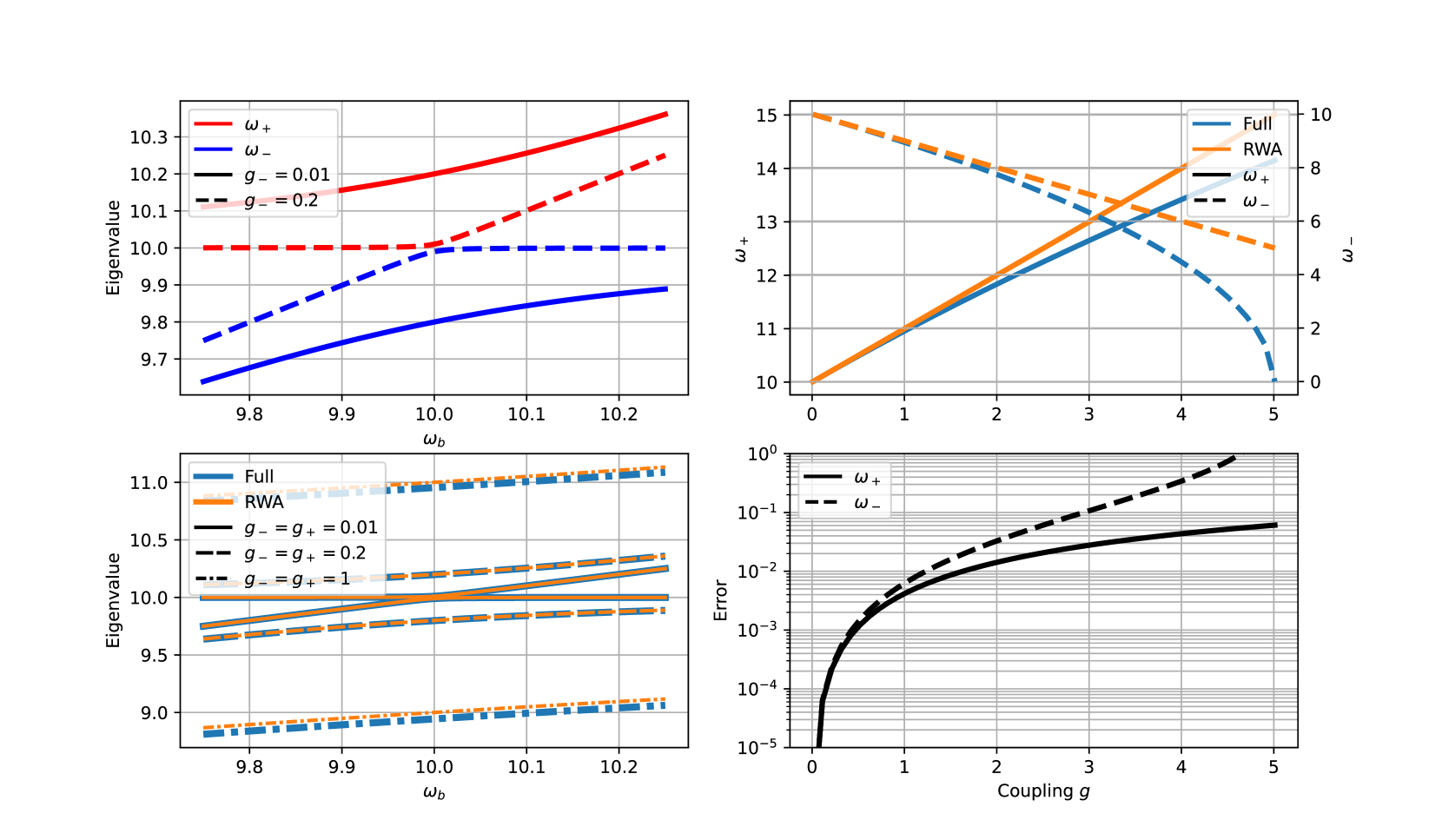
These eigenvalues are shown in Figure 8 a as a function of both and where we see the famous avoided level crossing.
The symmetry of Figure 8 a exists because we plot the normal frequencies against the frequency rather than the uncoupled frequency .
\levelstay
Accuracy of the rotating wave approximation
How accurate are the RWA eigenvalues plotted in Figure 8 a?
In Figure 8 b We compare the full coupled resonator eigenvalues against the RWA, working in the case that either or is zero so that .
For and the curves are visually indistinguishable.
For the curves just begin to separate, suggesting that the RWA begins to break down when the coupling is on the order of 10% of the frequencies of the coupled resonators.
Figure 8 c shows the eigenvalues taken at the avoided level crossing () and Figure 8 d shows the relative error of the RWA at the avoided level crossing.
Figure 8: Eigenvalues of the coupled resonator system. a) Eigenvalues as a function of for . b) Full eigenvalues (i.e. not taking the RWA) compared with the RWA. Here and are taken to be equal as appropriate for resonators coupled through only one of their conjugate variables, i.e. either flux or charge. c) Full and RWA eigenvalues at the avoided level crossing defined by . d) Relative error of the RWA.
\levelup
Coupled transmission lines
Kirchhoff’s laws for the circuit shown in Fig. 7 b are
In the limit , these equations become differential equations
(42)
Assuming sinusoidal time dependence at frequency , and therefore converting time derivatives to , these equations can be written in matrix form as 555The choice of sign in makes positive values of the wave vector correspond to right-moving waves.
(43)
If we convert to the ingoing and outcoming wave amplitudes
(44)
the equations of motion take the form
(45)
where is the wave vector and
(46)
\levelstay
Balanced coupling with nonlinear oscillators
In the main text we showed that the non-RWA terms and can be exactly canceled from the Hamiltonian of two coupled linear oscillators by balancing the electric and magnetic couplings.
In this section we analyze the case where one of the oscillators is a transmon qubit (a weakly nonlinear oscillator), while the other resonator is the qubit readout resonator, assumed to be a linear oscillator.
In contrast to the linear case, we will show that, in the nonlinear case, new non-RWA terms appear that cannot be simultaneously canceled under the balanced coupling condition.
In this section, we use a quantum description throughout.
We use the following approximate Hamiltonian for the transmon qubit [32]
(47)
where and are the (bare) qubit annihilation and creation operators, respectively.
is the plasma frequency, where and are respectively the charging and Josephson energies. is a dimensionless parameter characterizing the strength of the qubit nonlinearity ().
Typically for a transmon qubit, is of order of .
Here we define the dimensionless charge () and flux () operators of the qubit as
(48)
These dimensionless operators are normalized differently than and in the main text; in particular here .
The qubit readout resonator is assumed to be linear with Hamiltonian equal to , where and are the photon annihilation and creation operators.
The dimensionless charge and flux operators for the readout resonator are
(49)
The coupling between the two oscillators is similar to the electric-magnetic coupling discussed in the main text,
(50)
The balanced coupling condition reads as .
The analysis of the non-RWA terms is carried out in the eigenbasis of each oscillator.
We denote the eigenbasis of the transmon qubit by , where .
We can use perturbation theory to obtain the qubit eigenstates in terms of the bare qubit states [32] and determine the unitary operator that relates them,
(51)
To first order in , is given by ( is the identity operator)
(52)
Using Eq. (52), the qubit eigenstates , to first order in , are given by
In the qubit eigenstate basis, the annihilation operator transforms into the operator , which, to first order in , is given by
(54)
Equation (54) is useful to compute the matrix elements as the latter can be rewritten
(55)
Similarly, in the qubit eigenstate basis, the charge and flux operators are
(56)
(57)
and the coupling Hamiltonian becomes
(58)
Let us assume the balanced coupling condition holds, i.e. .
After inserting Eqs. (56)–(57) into Eq. (58), we find that the coupling Hamiltonian still includes non-RWA terms and can be written as
(59)
where
is the desired RWA coupling between the eigenstates and , belonging to the same RWA-strip with excitations [32], where indicates the number of photons in the readout resonator (an RWA-strip with excitations is defined as the subspace of states such that ).
The non-RWA terms in the coupling are given by
(60)
There are two types of non-RWA terms in .
The first type of non-RWA terms include the terms and (as well as their Hermitian-conjugated terms) that couple states of two RWA-strips separated by 2 excitations.
The second type of non-RWA terms are and that couple RWA-strips separated by 4 excitations [32].
These non-RWA couplings open the way to measurement-induced transitions (MIST) between, e.g., the qubit ground state to high-energy qubit eigenstates during qubit readout.
It is not possible to find a suitable operation point that eliminates all non-RWA terms.
More generally, we investigate the matrix elements involved in moving the system from one RWA strip to another one with two more excitations.
The matrix elements of involved in the transition are
(61)
(62)
and the matrix elements in involved in the transition are
(63)
(64)
References
Krantz et al. [2019]P. Krantz, M. Kjaergaard,
F. Yan, T. P. Orlando, S. Gustavsson, and W. D. Oliver, A quantum engineer’s guide to superconducting qubits, Appl. Phys. Rev. 6, 021318 (2019).
Blais et al. [2020]A. Blais, A. L. Grimsmo,
S. M. Girvin, and A. Wallraff, Circuit quantum electrodynamics, (2020), arXiv:2005.12667 .
Lecocq et al. [2017]F. Lecocq, L. Ranzani,
G. Peterson, K. Cicak, R. Simmonds, J. Teufel, and J. Aumentado, Nonreciprocal microwave signal processing with a field-programmable
josephson amplifier, Phys. Rev. Appl. 7, 024028 (2017).
Peterson et al. [2017]G. A. Peterson, F. Lecocq,
K. Cicak, R. W. Simmonds, J. Aumentado, and J. D. Teufel, Demonstration of efficient nonreciprocity in a microwave
optomechanical circuit, Phys. Rev. X 7 (2017).
Ranzani and Aumentado [2015]L. Ranzani and J. Aumentado, Graph-based analysis of
nonreciprocity in coupled-mode systems, New J. Phys. 17, 023024 (2015).
Louisell [1960]W. H. Louisell, Parametric and coupled
mode electronics (John Wiley & Sons, Inc., 1960).
Sank et al. [2016]D. Sank, Z. Chen, M. Khezri, J. Kelly, R. Barends, B. Campbell, Y. Chen, B. Chiaro, A. Dunsworth,
A. Fowler, E. Jeffrey, E. Lucero, A. Megrant, J. Mutus, M. Neeley, C. Neill, P. J. J. O’Malley, C. Quintana, P. Roushan,
A. Vainsencher, T. White, J. Wenner, A. N. Korotkov, and J. M. Martinis, Measurement-induced state transitions in a superconducting qubit: Beyond the
rotating wave approximation, Phys. Rev. Lett. 117, 190503 (2016).
Schuster et al. [2005]D. I. Schuster, A. Wallraff,
A. Blais, L. Frunzio, R.-S. Huang, J. Majer, S. M. Girvin, and R. J. Schoelkopf, ac stark shift and dephasing of a superconducting qubit strongly coupled to
a cavity field, Phys. Rev. Lett. 94, 123602 (2005).
Wallraff et al. [2004]A. Wallraff, D. I. Schuster, A. Blais,
L. Frunzio, R.-S. Huang, J. Majer, S. Kumar, S. M. Girvin, and R. J. Schoelkopf, Strong
coupling of a single photon to a superconducting qubit using circuit quantum
electrodynamics, Nature 431, 162 (2004).
Blais et al. [2004]A. Blais, R.-S. Huang,
A. Wallraff, S. Girvin, and R. J. Schoelkopf, Cavity quantum electrodynamics for superconducting
electrical circuits: An architecture for quantum computation, Phys. Rev. A 69, 062320 (2004).
Khezri et al. [2016]M. Khezri, E. Mlinar,
J. Dressel, and A. N. Korotkov, Measuring a transmon qubit in circuit qed: Dressed
squeezed states, Phys. Rev. A 94, 012347 (2016).
Zeuch et al. [2020]D. Zeuch, F. Hassler,
J. J. Slim, and D. P. DiVincenzo, Exact rotating wave approximation, Ann. Phys. 423, 168327 (2020).
Note [1] and
are the flux and charge zero point fluctuations in the ground state of the
quantum LC resonator.
Zhang et al. [2021]H. Zhang, S. Chakram,
T. Roy, N. Earnest, Y. Lu, Z. Huang, D. Weiss,
J. Koch, and D. I. Schuster, Universal fast-flux control of a coherent,
low-frequency qubit, Phys. Rev. X 11, 011010 (2021).
Najera-Santos et al. [2024]B.-L. Najera-Santos, R. Rousseau, K. Gerashchenko, H. Patange, A. Riva,
M. Villiers, T. Briant, P.-F. Cohadon, A. Heidmann, J. Palomo, et al., High-sensitivity ac-charge detection with a
mhz-frequency fluxonium qubit, Phys. Rev. X 14, 011007 (2024).
Connolly and Kurlovich [tion]T. Connolly and P. Kurlovich, (In
preparation).
Campbell et al. [2020]D. L. Campbell, Y.-P. Shim,
B. Kannan, R. Winik, D. K. Kim, A. Melville, B. M. Niedzielski, J. L. Yoder, C. Tahan, S. Gustavsson, and W. D. Oliver, Universal nonadiabatic control of
small-gap superconducting qubits, Phys. Rev. X 10, 041051 (2020).
Rower et al. [2024]D. A. Rower, L. Ding,
H. Zhang, M. Hays, J. An, P. M. Harrington, I. Rosen, J. M. Gertler, T. M. Hazard, B. M. Niedzielski, M. E. Schwartz, S. Gustavsson, K. Serniak,
J. A. Grover, and W. D. Oliver, Suppressing counter-rotating errors for fast
single-qubit gates with fluxonium, In preparation (2024).
Wallraff et al. [2005]A. Wallraff, D. Schuster,
A. Blais, L. Frunzio, J. Majer, M. Devoret, S. Girvin, and R. Schoelkopf, Approaching unit visibility for control of a superconducting qubit with
dispersive readout, Phys. Rev. Lett. 95, 060501 (2005).
Jeffrey et al. [2014]E. Jeffrey, D. Sank,
J. Y. Mutus, T. C. White, J. Kelly, R. Barends, Y. Chen, Z. Chen, B. Chiaro,
A. Dunsworth, A. Megrant, P. J. J. O’Malley, C. Neill, P. Roushan, A. Vainsencher, J. Wenner, A. N. Cleland, and J. M. Martinis, Fast
accurate state measurement with superconducting qubits, Phys. Rev. Lett. 112, 190504 (2014).
Heinsoo et al. [2018]J. Heinsoo, C. K. Andersen, A. Remm,
S. Krinner, T. Walter, Y. Salathé, S. Gasparinetti, J.-C. Besse, A. Potočnik, A. Wallraff, and C. Eichler, Rapid high-fidelity
multiplexed readout of superconducting qubits, Phys. Rev. Appl. 10, 034040 (2018).
Khezri et al. [2023]M. Khezri, A. Opremcak,
Z. Chen, K. C. Miao, M. McEwen, A. Bengtsson, T. White, O. Naaman, D. Sank, A. N. Korotkov, Y. Chen, and V. Smelyanskiy, Measurement-induced
state transitions in a superconducting qubit: Within the rotating-wave
approximation, Phys. Rev. Appl. 20, 054008 (2023).
Shillito et al. [2022]R. Shillito, A. Petrescu,
J. Cohen, J. Beall, M. Hauru, M. Ganahl, A. G. Lewis, G. Vidal, and A. Blais, Dynamics of transmon ionization, Phys. Rev. Appl. 18, 034031 (2022).
Dumas et al. [2024]M. F. Dumas, B. Groleau-Paré, A. McDonald, M. H. Muñoz-Arias, C. Lledó, B. D’Anjou, and A. Blais, Unified picture of measurement-induced ionization
in the transmon, arXiv:2402.06615 (2024).
Cohen et al. [2023]J. Cohen, A. Petrescu,
R. Shillito, and A. Blais, Reminiscence of classical chaos in driven
transmons, PRX Quantum 4, 020312 (2023).
Miao et al. [2023]K. C. Miao, M. McEwen,
J. Atalaya, D. Kafri, L. P. Pryadko, A. Bengtsson, A. Opremcak, K. J. Satzinger, Z. Chen, P. V. Klimov, et al., Overcoming leakage in quantum error correction, Nat. Phys. 19, 1780 (2023).
Kounalakis et al. [2018]M. Kounalakis, C. Dickel,
A. Bruno, N. Langford, and G. Steele, Tuneable hopping and nonlinear cross-kerr interactions in
a high-coherence superconducting circuit, npj Quant. Inf. 4 (2018).
Note [2] where
is the gyromagnetic ratio, so has
dimensions of frequency.
Note [3]This approximation leaves out terms proportional to which can usually be ignored under assumptions similar to the
RWA.
Note [4]Because matrix transposition and inversion commute, and
because the matrix is symmetric, we can bring from the bra
onto the ket for free.
Note [5]The choice of sign in makes positive values of
the wave vector correspond to right-moving waves.
Khezri [2018]M. Khezri, Dispersive Measurement
of Superconducting Qubits (PhD Thesis, University
of California Riverside, 2018).