Hofstadter spectrum in a semiconductor moiré lattice

Abstract

Recently, the Hofstadter spectrum of a twisted $\mathrm{WSe_{2}/MoSe_{2}}$ heterobilayer has been observed in experiment [C. R. Kometter, et al. Nat. Phys. 19, 1861 (2023)], but the origin of Hofstadter states remains unclear. Here, we present a comprehensive theoretical interpretation of the observed Hofstadter states by calculating its accurate Hofstadter spectrum. We point out that the valley Zeeman effect, a unique feature of the transition metal dichalcogenide (TMD) materials, plays a crucial role in determining the shape of the Hofstadter spectrum, due to the narrow bandwidth of the moiré bands. This is distinct from the graphene-based moiré systems. We further predict that the Hofstadter spectrum of the moiré flat band, which was not observed in experiment, can be observed in the same system with a larger twist angle $2^{\circ}\lesssim\theta\lesssim 3^{\circ}$. Our theory paves the way for further studies of the interplay between the Hofstadter states and correlated insulting states in such moiré lattice systems.

Introduction.—The Hofstadter spectrum, an extraordinary self-similar fractal spectrum, emerges in two-dimensional electron systems when exposed to both periodic potential and perpendicular magnetic fieldsHofstadter (1976). It is of special interest because it is not only a very fundamental issue in quantum theory of solids, but also one of the earliest discovered quantum fractals in physics. To obtain the Hofstadter spectrum, it is required that the magnetic length ($\ell_{B}=\sqrt{\hbar/eB}$) should be comparable with the length of the unit cell. This requirement makes the moiré systems an ideal platform for realizing such novel fractal energy spectrum, because the large moiré unit cell facilitates the manifestation of Hofstadter states in moderate magnetic fieldsYang and Zhang (2022); Bistritzer and MacDonald (2011); Crosse et al. (2020); Hejazi et al. (2019); Lian et al. (2020); Kometter et al. (2023); Moon and Koshino (2012); Chen et al. (2014); Wang et al. (2012); Zhang et al. (2019); Yu et al. (2014); Wang et al. (2015a); Krishna Kumar et al. (2018); Spanton et al. (2018); Chen et al. (2017); Yang et al. (2016); Lu et al. (2021, 2020); Das et al. (2021); Imran et al. (2023); Wu et al. (2021); Ponomarenko et al. (2013); Burg et al. (2022); He et al. (2021); Shen et al. (2020); Forsythe et al. (2018); Dean et al. (2013); Hao et al. (2021); Hunt et al. (2013); Schmidt et al. (2014); Yankowitz et al. (2019); Wang et al. (2015b); Rademaker et al. (2020); Park et al. (2021); Xie et al. (2021); Saito et al. (2021); Lu et al. (2019); Das et al. (2022); Herzog-Arbeitman et al. (2022); Burg et al. (2019).

Recently, a remarkable experiment reports the observation of the Hofstadter states in a twisted transition metal dichalcogenide (TMD) heterobilayer ($\mathrm{WSe_{2}/MoSe_{2}}$), revealing a rich phase diagram of interpenetrating Hofstadter states and charge-ordered states through local electronic compressibility measurementsKometter et al. (2023). The twisted TMD heterobilayer has received significant attention in the last few years, because it can be equivalently mapped into a triangle lattice Hubbard model with adjustable bandwidth and Hubbard interaction, making such a semiconductor moiré lattice an ideal platform for simulating strongly correlated electron statesWu et al. (2018a); Seyler et al. (2019); Jin et al. (2019); Tran et al. (2019); Alexeev et al. (2019); Wu et al. (2018b, 2017); Paul et al. (2022); Xie et al. (2023); Tang et al. (2020); Li et al. (2021a); Zhao et al. (2023); Xu et al. (2020); Huang et al. (2021); Regan et al. (2020); Jin et al. (2021); Shabani et al. (2021); Li et al. (2021b); Jin et al. (2018); Tang et al. (2022); Xie et al. (2022); Devakul and Fu (2022); Pan et al. (2022). This experiment reveals that, in the presence of a strong magnetic field, the twisted TMD heterobilayer provides unprecedented opportunities for systematic exploration of the interplay between the Hofstadter states and the strongly correlated states in artificial electron lattices. However, from a theoretical standpoint, there is still a lack of quantitative understanding of this crucial experiment. Most importantly, the origin of Hofstadter states in twisted TMD heterobilayers still remains unclear.

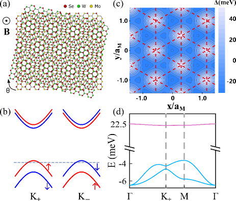
Figure 1: (a) Schematic of twisted $\mathrm{WSe_{2}}/\mathrm{MoSe_{2}}$ heterobilayer. $\theta$ is the twist angle and $\mathbf{B}$ denotes the perpendicular magnetic field. (b) Band structure of $\mathrm{WSe_{2}}$ monolayer near $\mathrm{K_{+}}$ and $\mathrm{K_{-}}$ points. Red (Blue) represents for up (down) spin. (c) Moiré periodic potential $\Delta(\mathbf{r})$. (d) The first three moiré bands calculated by the continuum model at twist angle $\theta=1.33^{\circ}$. Purple (blue) lines are for the moiré $s$-bands ($p_{x,y}$-bands).

In this work, we present a comprehensive theoretical interpretation of the observed Hofstadter states in the twisted TMD heterobilayer by directly calculating the Hofstadter spectrum. The key finding of our theory is that the valley Zeeman effectRobert et al. (2021); Kormányos et al. (2015); Deilmann et al. (2020); Woźniak et al. (2020); Xuan and Quek (2020); Rostami and Asgari (2015); Rybkovskiy et al. (2017), a distinctive characteristic of TMD materials, plays a crucial role in determining the Hofstadter spectrum in such system, which is essentially different from graphene-based moiré systemsHejazi et al. (2019); Crosse et al. (2020); Lian et al. (2020). Once the valley Zeeman term is properly considered, the single particle Hofstadter spectrum can well interpret almost all the experimental observations regarding the Hofstadter states. In fact, the observed Hofstadter spectrum in $\mathrm{WSe_{2}/MoSe_{2}}$ bilayer can be roughly approximated as that of a spinful $p_{x,y}$-orbital triangle lattice. The tight-binding model is given in the supplementary materials . Finally, we predict the primary characteristics of the Hofstadter spectrum of the moiré flat band, which has not been observed in the current experiment but should be detected with a larger twist angle $2^{\circ}\lesssim\theta\lesssim 3^{\circ}$. Our theory interprets the origin of the observed Hofstadter states in the twisted TMD heterobilayer, while also paving the way for quantitative understanding of the intriguing interplay between the Hofstadter states and the correlated electron states in TMD moiré lattices.

Model.—We consider a twisted $\mathrm{WSe_{2}/MoSe_{2}}$ heterobilayer in the presence of a perpendicular magnetic field $\mathbf{B}=(0,0,B_{z})$ with a twist angle $\theta$, as illustrated in Fig. 1(a). Fig. 1(b) is the schematic of the bands of $\mathrm{WSe_{2}}$ monolayer at the $K_{+}$ and $K_{-}$ valley near $E_{F}$. Due to the strong spin-orbit coupling, the topmost valence bands have opposite spin at the two valleys, i.e. the spin-valley lockingXiao et al. (2012); Liu et al. (2015); Zeng et al. (2012); Cao et al. (2012). Meanwhile, the $\mathrm{MoSe_{2}}$ monolayer behaves like a twist angle dependent moiré periodic potential applied on the $\mathrm{WSe_{2}}$ monolayer. So, considering the topmost valence band at one valley, the Hamiltonian is

$$H =-\frac{(\mathbf{p}+e\mathbf{A})^{2}}{2m^{\ast}}+\Delta(\mathbf{r})-\mathbf{m}\cdot\mathbf{B}$$ (1)

where the first term is the kinetic energy, $\Delta(\mathbf{r})$ is the moiré periodic potential and the last term represents the effective Zeeman effect.

Here, $\Delta(\mathbf{r})$ is of the moiré period $a_{M}\approx a_{0}/\theta$, where $a_{0}$ is the lattice constant of $\mathrm{WSe_{2}}$. Since the TMD monolayer has threefold-rotational symmetry, $\Delta(\mathbf{r})$ can be well approximated by only six moiré reciprocal lattice vectors

$$\Delta(\mathbf{r}) =\sum^{6}_{j=1}V(\mathbf{b}_{j})\mathrm{exp}(i\mathbf{b}_{j}\cdot\mathbf{r}),$$ (2)

with $\mathbf{b_{j}}=\frac{4\pi}{\sqrt{3}a_{M}}(\cos{\frac{\pi(j-1)}{3}},\sin{\frac{\pi(j-1)}{3}})$ and $V(\mathbf{b_{j}})=V\mathrm{exp}[(-1)^{(j-1)}i\psi]$. Here, $V$ and $\psi$ are two fitting parameters for the moiré potential. For the AA-stacked $\mathrm{WSe_{2}}/\mathrm{MoSe_{2}}$ bilayer with $\theta=1.33^{\circ}$, we use the parameters: $(V,\psi)=(9\mathrm{meV},-125.1^{\circ})$, $a_{M}=13.5\mathrm{nm}$ and $m^{\ast}=0.5m_{0}$. Note that, unless otherwise specified, we always set $\theta=1.33^{\circ}$, which is the value in the experimentKometter et al. (2023).

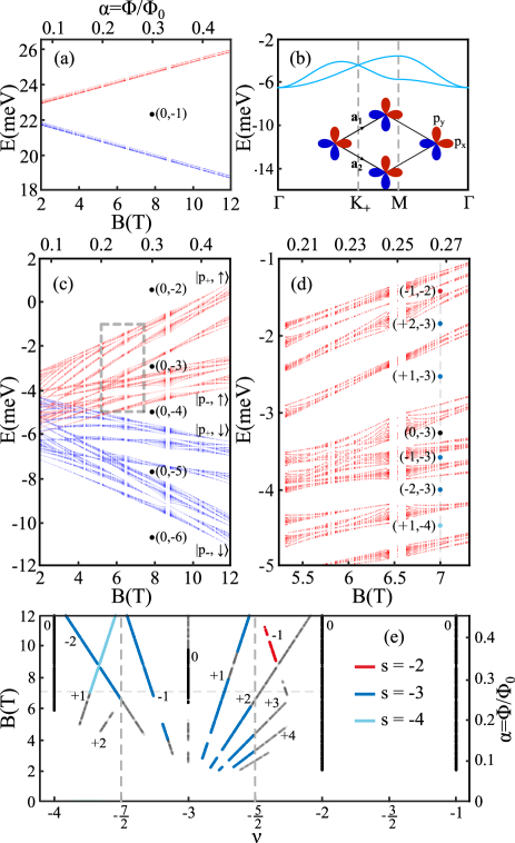
Figure 2: Hofstadter spectrum of a twisted $\mathrm{WSe_{2}}/\mathrm{MoSe_{2}}$ heterobilayer with $\theta=1.33^{\circ}$. (a) is for moiré $s$-band and (c) is for moiré $p$-bands. Red (blue) represents up (down) spin. $(t,s)$ for the visible gaps are labeled. (b) is the schematic and band structure of a $p_{x,y}$-orbital triangular lattice, which corresponds to the moiré $p$-bands. (d) is the magnified version of the Hofstadter spectrum within the dashed box in (c). (e) Wannier diagram of moiré $p$-bands. The minimum energy resolution for gaps is $0.12$ meV. $t$ of each Hofstadter state is labeled, and $s$ is denoted by color.

Such moiré potential actually forms a triangle lattice, as shown in Fig. 1(c), where lattice sites correspond to the maxima of the moiré potential. The holes are localized around the lattice sites, forming artificial atoms of the triangle lattice. The energy bands with $\mathbf{B}=0$ are plotted in Fig. 1(d). The first band (purple line) is just the well-known moiré flat band, which is also called moiré $s$-band here because it corresponds to the $s$-band of the triangle lattice. The other two dispersive bands (blue lines) are called moiré $p$-bands, due to the correspondence to the $p$-bands of the triangle lattice forming by the artificial $p_{x,y}$-orbitals. Here, $s$-orbital refers to the first orbital (for holes) confined by the moiré potential at the lattice sites. $p_{x,y}$-orbitals have similar definitions.

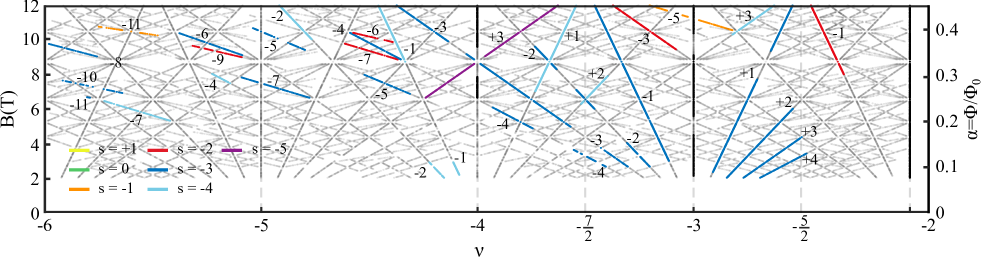
Figure 3: Wannier diagram with higher energy resolution. Gray lines are the calculated gap trajectories. The gap trajectories observed in experiment are marked in color, where color denotes $s$ of each gap, and $t$ are labeled as well. The minimum energy resolution for gaps is $0.004$ meV.

When a perpendicular magnetic field is applied on a TMD monolayer, there are two effects of the magnetic field, which are of equal importance for the Hofstadter spectrum. One is the formation of Landau levels (LL), represented by the Peierls substitution, see the first term in Eq. (1). The other is a valley-dependent Zeeman splitting, resulting from the spin and orbital magnetic momentum of the valence electrons, i.e. the last term in Eq. (1). Here, the total magnetic momentum includes contributions from both orbital and spin magnetic momentum, which can be described by an effective $g$-factor $g^{\tau}_{\mathrm{eff}}$

$$\mathbf{m}\cdot\mathbf{B}=(\mathbf{m}^{\tau}_{\mathrm{orb}}+\mathbf{m}^{\tau}_{\mathrm{spin}})\cdot\mathbf{B}=-g^{\tau}_{\mathrm{eff}}\mu_{B}B_{z}$$ (3)

where $\tau=\pm$ is the valley index. As well known, the orbital magnetic momentum of the valence electron in TMD are related to its Berry curvature, which have opposite sign in the two valleysDeilmann et al. (2020); Rybkovskiy et al. (2017); Xiao et al. (2012); Woźniak et al. (2020); Xuan and Quek (2020); Rostami and Asgari (2015). Meanwhile, the spin of the valence electron in the two valleys are opposite as well due to the strong spin-orbit couplingKormányos et al. (2015); Deilmann et al. (2020); Xiao et al. (2012); Woźniak et al. (2020); Robert et al. (2021). So, in the presence of magnetic field, the valence electrons in the two valleys have opposite Zeeman shifts, i.e. $g^{\tau}_{\mathrm{eff}}$ with opposite sign, which is so-called valley Zeeman effect. The $g^{\tau}_{\mathrm{eff}}$ of the $\mathrm{WSe_{2}}$ monolayer can be calculated with various theoretical methods like DFT or tight-binding model, with values ranging from $1.19$ to $6.1$Kormányos et al. (2015); Deilmann et al. (2020); Rybkovskiy et al. (2017); Woźniak et al. (2020); Robert et al. (2021); Xuan and Quek (2020). However, $g^{\tau}_{\mathrm{eff}}$ in the moiré heterobilayer should differ from that in TMD monolayer due to the modifications of orbital magnetic momentum caused by the moiré potential. Here, we choose $g^{\tau}_{\mathrm{eff}}=5.2$ for valley $K_{+}$ ($\tau=+1$), which is in good agreement with the experimental observations. The details in the determination of the $g$-factor are given in the supplementary materials .

Hofstadter spectrum.—To calculate the Hofstadter spectrum, we use the Landau gauge $\mathbf{A}=(0,xB_{z},0)$ and diagonalize the Hamiltonian (1) with the wave functions of LL $\ket{n,k_{y}}$ as the basisPfannkuche and Gerhardts (1992), where

$$\ket{n,k_{y}}=L_{y}^{1/2}\mathrm{exp}(ik_{y}y)\phi_{n}(x-x_{0}).$$ (4)

corresponds to the LL with $E_{n}=-\hbar\omega_{c}(n+\frac{1}{2})$, $\phi_{n}(x-x_{0})$ is the normalized oscillator function and $x_{0}=-\ell_{B}^{2}k_{y}$. The matrix element of the moiré periodic potential can be calculated with the formula

$$\bra{n^{\prime},k_{y}^{\prime}} \mathrm{exp}(i\mathbf{q}\cdot\mathbf{r})\ket{n,k_{y}}$$ (5)

$$=\delta_{k_{y}^{\prime},k_{y}+q_{y}}\mathrm{exp}[-\frac{i}{2}\ell_{B}^{2}q_{x}(k_{y}^{\prime}+k_{y})]\mathcal{L}_{n^{\prime}n}(\mathbf{q})$$

with

$$\mathcal{L}_{n^{\prime},n}(\mathbf{q})= (m!/M!)^{1/2}i^{\mid n^{\prime}-n\mid}[(q_{x}+iq_{y})/q]^{n-n^{\prime}}$$ (6)

$$\hfill\times e^{-\frac{1}{2}Q}Q^{\frac{1}{2}\mid n^{\prime}-n\mid}L_{m}^{(\mid n^{\prime}-n\mid)}(Q),$$

where $\mathbf{q}=(q_{x},q_{y})$, $q=|\mathbf{q}|$ and $Q=\frac{1}{2}\ell_{B}^{2}q^{2}$. $m$ and $M$ are the minimum and the maximum of $n^{\prime}$ and $n$. $L^{(\alpha)}_{j}(Q)$ is the associated Laguerre polynomial. Here, the inter-LL matrix elements need to be considered. The calculation details are given in the supplementary materials .

In such semiconductor moiré superlattice, a twist angle $\theta=1.33^{\circ}$ gives $a_{M}\approx 13.5$ nm, so that the requirement to realize Hofstadter spectrum $\ell_{B}\lesssim a_{M}$ desires $B\gtrsim 3.6$ T. In this situation, the applied magnetic field will split the moiré bands to form a fractal energy spectrum, i.e. the Hofstadter spectrum. We plot the calculated Hofstadter spectrum of the first three moiré bands in Fig. 2. Fig 2(a) shows the Hofstadter spectrum of the moiré $s$-band, which corresponds to an $s$-orbital triangle lattice model. The Hofstadter spectra for the up and down spin (or $K_{\pm}$ valleys) are split by the effective Zeeman term, where the red (blue) lines in Fig. 2(a) represent up (down) spin. With $\theta=1.33^{\circ}$, the moiré $s$-band is a flat band with a very narrow bandwidth, see Fig. 1(d). Consequently, the gaps between the Hofstadter minibands are very tiny, which are hard to detect in experiment.

When $\nu<-2$ ($\nu$ is the hole filling per moiré unit cell), the Fermi level $E_{F}$ shifts to the moiré $p$-bands. The Hofstadter spectrum of the moiré $p$-bands is given in Fig. 2(c). First of all, the most notable feature of the Hofstadter spectrum is its division into four distinct sets as the magnetic field increases. This can be intuitively understood from the equivalent lattice model. As illustrated in Fig. 2(b), the moiré $p$-bands correspond to a spinful $p_{x,y}$-orbital triangle lattice, which can be described by four basis functions $\{\ket{p_{\pm},\uparrow},\ket{p_{\pm},\downarrow}\}$ with $\ket{p_{\pm}}=\ket{p_{x}}\pm i\ket{p_{y}}$. Here, the spin of the lattice model is just the valley degree of freedom of the moiré heterobilayer, so that the valley Zeeman term in Eq. (3) becomes an effective spin Zeeman splitting in the lattice model, leading to the splitting of the up (red lines) and down (blue lines) spin when a magnetic field is applied. Meanwhile, the artificial $p$-orbitals have their own orbital magnetic momentum, which means that the $\ket{p_{\pm},\uparrow}$ orbitals will be split further. Therefore, the Hofstadter spectrum of the up spin (red lines) is partitioned into two distinct sets: the upper one for $\ket{p_{+},\uparrow}$ orbital and the lower one for $\ket{p_{-},\uparrow}$. The case of down spin (blue lines) is similar. Thus, we finally get four different sets of Hofstadter spectrum for the moiré $p$-bands.

The gaps between the Hofstadter minibands in the $p$-band spectrum are significantly larger than those in the moiré $s$-bands, since the moiré $p$-bands are more dispersive than the flat $s$-band, as illustrated in Fig. 1(d). If we set $0.12$ meV as the minimum energy resolution, the detectable minigaps are marked on the enlarged Hofstadter spectrum, see Fig. 2(d). As well known, the gaps of the Hofstadter spectrum, i.e. incompressible Hofstadter states, can be described by two topological integers $(t,s)$ through the Diophantine equationThouless et al. (1982)

$$n/n_{0}=t(\phi/\phi_{0})+s,$$ (7)

which correspond to linear trajectories in the Wannier diagramWannier (1978). Here, $n/n_{0}$ and $\phi/\phi_{0}$ are the normalized carrier density and magnetic flux, respectively ($n_{0}$ is the carrier density of a completely filled Bloch band and $\phi_{0}$ is the magnetic flux quantum). $t$ reflects the Hall conductivity $\sigma_{xy}=te^{2}/h$ associated with each minigap of the Hofstadter spectrum, and $s$ represents the Bloch band filling at each gapThouless et al. (1982); Koshino and Ando (2006); Streda (1982); Springsguth et al. (1997). The calculated Wannier diagram is plotted in Fig. 2(e). In the region of $-2<\nu<-1$, $E_{F}$ falls within the moiré s-band and there are no observable minigaps in the Hofstadter spectrum. Thus, no corresponding linear trajectories are found in the Wannier diagram. The most intriguing region is $-4<\nu<-2$, which corresponds to the $p$-band Hofstadter spectrum arising from the $\ket{p_{\pm},\uparrow}$ orbitals, i.e. the red lines in Fig. 2(c) and (d). The observable gaps of the Hofstadter spectrum here do give rise to linear trajectories in the Wannier diagram. As shown in Fig. 2(e), with a small magnetic field ($B<4$ T), the gap trajectories mainly stem from $s=-3$, resembling an asymmetric Landau fan that is denser in the low hole filling region. When $B>6$ T, obvious Hofstadter states with $s=-2,-3,-4$ appear. The $(t,s)$ of each minigaps are given in Fig. 2(d) and (e) accordingly. In Fig. 2(d), we see that the Hall conductivity exhibits a non-monotonic behavior as a function of $E_{F}$ in the presence of a strong magnetic field, which is the characteristic feature of the Hofstadter spectrum. Note that the Wannier diagram in Fig. 2(e) almost perfectly reproduces the Hofstadter states observed in experiment. The comparison with the experimental observation is given in the supplementary materials .

The Wannier diagram in Fig. 2(e) can be well interpreted by the single particle Hofstadter spectrum. First, with a small $B$, the effective Zeeman splitting is not large enough, so that the Hofstadter spectrum of the $\ket{p_{-},\uparrow}$ overlaps with that of the $\ket{p_{+},\downarrow}$, as shown in Fig. 2(c). Thus, the gaps will gradually disappear as hole filling increases, resulting in the asymmetric Landau fan around $\nu=-3$ in the Wannier diagram. Second, by increasing the magnetic field ($B>6$ T), the effective Zeeman splitting becomes large enough to separate the Hofstadter spectrum of different orbitals. As a result, the gap trajectories can be found in the region of large hole filling ($\nu<-3$) in Fig. 2(e). Third, in the Wannier diagram, there are gap trajectories with $t=0$ at $\nu=-1,-2,-3,-4$ (the black vertical lines). From the energy spectrum in Fig. 2(c), we see that these vertical trajectories correspond to the band gaps between different orbitals, which are different from the cyclotron gaps resulting from the magnetic field. So, the Hall conductivity is zero ($t=0$) here.

The analysis above clearly indicates that the effective Zeeman splitting, resulting from both the spin and orbital magnetic momentum, plays a key role in determining the Hofstadter spectrum and the Wannier diagram. Proper Zeeman splitting ensures the correct order of the Hofstadter spectrum for different orbitals, which is crucial for the Wannier diagram. Therefore, the experiment in turn provides an accurate estimation of the magnitude of the Zeeman splitting in such a semiconductor moiré lattice.

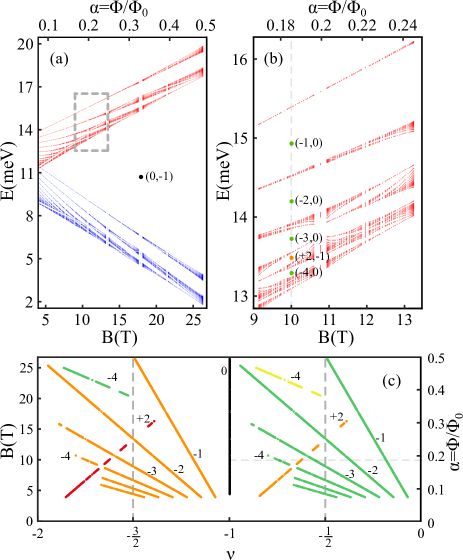
Figure 4: (a) Hofstadter spectrum of moiré $s$-bands at twist angle $\theta=2^{\circ}$. (b) is the magnified version of the Hofstadter spectrum within the dashed box in (a). $(t,s)$ for the visible gaps are labeled. (c) Wannier diagram of the moiré $s$-bands. The minimum energy resolution for gaps is $0.12$ meV. $t$ of main gaps trajectory are labeled. $s$ is denoted by color, which is the same as Fig. 3.

In experiment, higher precision measurements unveil a more intricate Hofstadter spectrum patternKometter et al. (2023). We thus calculate the Wannier diagram with higher energy resolution for the gaps ($0.004$ meV), while keeping all the system parameters unchanged. The results are plotted in Fig. 3, where the gray lines represent all the gap trajectories of the Hofstadter spectrum in the whole region $-6<\nu<-2$. As expected, almost all of the gap trajectories observed in the experiment can be found in the calculated Wannier diagram in Fig. 3, which are marked in color. At low field, the gap trajectories remain the Landau fan around $\nu=-3$, while more gaps with negative $t$ around $\nu=-3,-4$ become visible. At high fields, gap trajectories with $s=-1,-2,-3,-4,-5$ appear in the region of large hole filling, which originates from the fine structure of the Hofstadter spectrum.

Now, except for the correlation-induced charge-ordered states, almost all the Hofstadter states observed in the experiment are well explained by our single particle theory. But, it is worth noting that the energy resolution for the gaps used in our calculations in Fig. 3 is higher than what was claimed in the experiment, and the reason for this is currently unclear. Meanwhile, our calculation also shows that the calculated Hofstadter spectrum of the moiré $s$- and $p$-bands are quite like that of the triangle lattice.

Hofstadter spectrum of the moiré $s$-band.—With a twist angle $\theta=1.33^{\circ}$, the moiré $s$-band is extremely flat, so that the corresponding gaps in the Hofstadter spectrum are hard to detect even if the requirement $\ell_{B}\lesssim a_{M}$ is well satisfied. Thus, an intriguing question is whether it is possible to observe the $s$-band Hofstadter spectrum in such moiré semiconductor lattice system.

A natural way is to increase the twist angle, in order to get a large bandwidth. However, a larger twist angle means a smaller $a_{M}$, and the corresponding magnetic field required to achieve the Hofstadter spectrum becomes larger. Based on our numerical calculation, we predict that $2^{\circ}\lesssim\theta\lesssim 3^{\circ}$ is a reasonable region to observe the Hofstadter spectrum in experiment. The Hofstadter spectrum of the moiré $s$-bands in the same system with $\theta=2^{\circ}$ is plotted in Fig. 4(a) and (b). As we see, the Hofstadter spectrum of the up and down spin are split by the valley Zeeman term. Most importantly, under a reasonable magnetic field $B<20$ T, the gaps between the Hofstadter spectrum become visible and the corresponding $(t,s)$ are denoted in Fig. 4(b). Nonmonotonic variation of $t$ is observed here. The corresponding Wannier diagram is shown in Fig. 4(c), where the energy resolution of the gaps is the same as that in Fig. 2. We expect that the Hofstadter spectrum for the down spin (blue lines), i.e. the gap trajectories in the region $\-2<\nu<-1$ may be modified by the Hubbard U term in such moiré lattice. It is thus also a suitable platform to investigate the competition between the Hofstadter states and correlation-induced ordered states.

Summary.— In short, we interpret the origin of the Hofstadter states observed in a recent experiment by calculating its single particle Hofstadter spectrum. Unlike the graphene-based moiré systems, the valley Zeeman splitting plays a key role in determining the shape of the Hofstadter spectrum. The reason is that the bandwidth of the moiré bands here is very narrow, comparable to the valley Zeeman splitting. Our theory provides a good theoretical foundation for further studies of the competition between the Hofstadter states and correlated ordered states in semiconductor moiré lattice systems.

We thank Prof. Hua Chen and Wenyang Zhao for helpful discussions. This work was supported by the National Key Research and Development Program of China (No. 2022YFA1403501), and the National Natural Science Foundation of China(Grants No. 12141401, No. 11874160, No. 12204044).

References

- Hofstadter (1976) D. R. Hofstadter, Phys. Rev. B 14, 2239 (1976).
- Yang and Zhang (2022) W. Yang and G. Zhang, (2022), arXiv:2203.05821 .
- Bistritzer and MacDonald (2011) R. Bistritzer and A. MacDonald, Phys. Rev. B 84, 035440 (2011).
- Crosse et al. (2020) J. A. Crosse, N. Nakatsuji, M. Koshino, and P. Moon, Phys. Rev. B 102, 035421 (2020).
- Hejazi et al. (2019) K. Hejazi, C. Liu, and L. Balents, Phys. Rev. B 100, 035115 (2019).
- Lian et al. (2020) B. Lian, F. Xie, and B. A. Bernevig, Phys. Rev. B 102, 041402 (2020).
- Kometter et al. (2023) C. R. Kometter, J. Yu, T. Devakul, A. P. Reddy, Y. Zhang, B. A. Foutty, K. Watanabe, T. Taniguchi, L. Fu, and B. E. Feldman, Nat. Phys. 19, 1861–1867 (2023).
- Moon and Koshino (2012) P. Moon and M. Koshino, Phys. Rev. B 85, 195458 (2012).
- Chen et al. (2014) X. Chen, J. R. Wallbank, A. A. Patel, M. Mucha-Kruczyński, E. McCann, and V. I. Fal’ko, Phys. Rev. B 89, 075401 (2014).
- Wang et al. (2012) Z. Wang, F. Liu, and M. Chou, Nano Lett. 12, 3833 (2012).
- Zhang et al. (2019) Y.-H. Zhang, H. C. Po, and T. Senthil, Phys. Rev. B 100, 125104 (2019).
- Yu et al. (2014) G. Yu, R. Gorbachev, J. Tu, A. Kretinin, Y. Cao, R. Jalil, F. Withers, L. Ponomarenko, B. Piot, M. Potemski, et al., Nat. Phys. 10, 525 (2014).
- Wang et al. (2015a) L. Wang, Y. Gao, B. Wen, Z. Han, T. Taniguchi, K. Watanabe, M. Koshino, J. Hone, and C. R. Dean, Science 350, 1231 (2015a).
- Krishna Kumar et al. (2018) R. Krishna Kumar, A. Mishchenko, X. Chen, S. Pezzini, G. Auton, L. Ponomarenko, U. Zeitler, L. Eaves, V. Fal’ko, and A. Geim, Proc. Natl. Acad. Sci 115, 5135 (2018).
- Spanton et al. (2018) E. M. Spanton, A. A. Zibrov, H. Zhou, T. Taniguchi, K. Watanabe, M. P. Zaletel, and A. F. Young, Science 360, 62 (2018).
- Chen et al. (2017) G. Chen, M. Sui, D. Wang, S. Wang, J. Jung, P. Moon, S. Adam, K. Watanabe, T. Taniguchi, S. Zhou, M. Koshino, G. Zhang, and Y. Zhang, Nano Lett. 17, 3576 (2017).
- Yang et al. (2016) W. Yang, X. Lu, G. Chen, S. Wu, G. Xie, M. Cheng, D. Wang, R. Yang, D. Shi, K. Watanabe, T. Taniguchi, C. Voisin, B. Plaçais, Y. Zhang, and G. Zhang, Nano Lett. 16, 2387 (2016).
- Lu et al. (2021) X. Lu, B. Lian, G. Chaudhary, B. A. Piot, G. Romagnoli, K. Watanabe, T. Taniguchi, M. Poggio, A. H. MacDonald, B. A. Bernevig, and D. K. Efetov, Proc. Natl. Acad. Sci. USA 118, e2100006118 (2021).
- Lu et al. (2020) X. Lu, J. Tang, J. R. Wallbank, S. Wang, C. Shen, S. Wu, P. Chen, W. Yang, J. Zhang, K. Watanabe, T. Taniguchi, R. Yang, D. Shi, D. K. Efetov, V. I. Fal’ko, and G. Zhang, Phys. Rev. B 102, 045409 (2020).
- Das et al. (2021) I. Das, X. Lu, J. Herzog-Arbeitman, Z.-D. Song, K. Watanabe, T. Taniguchi, B. A. Bernevig, and D. K. Efetov, Nat. Phys. 17, 710 (2021).
- Imran et al. (2023) M. Imran, P. M. Haney, and Y. Barlas, Phys. Rev. B 108, 085417 (2023).
- Wu et al. (2021) Q. Wu, J. Liu, Y. Guan, and O. V. Yazyev, Phys. Rev. Lett. 126, 056401 (2021).
- Ponomarenko et al. (2013) L. A. Ponomarenko, R. V. Gorbachev, G. L. Yu, D. C. Elias, R. Jalil, A. A. Patel, A. Mishchenko, A. S. Mayorov, C. R. Woods, J. R. Wallbank, M. Mucha-Kruczynski, B. A. Piot, M. Potemski, I. V. Grigorieva, K. S. Novoselov, F. Guinea, V. I. Fal’ko, and A. K. Geim, Nature 497, 594 (2013).
- Burg et al. (2022) G. W. Burg, E. Khalaf, Y. Wang, K. Watanabe, T. Taniguchi, and E. Tutuc, Nat. Mater. 21, 884 (2022).
- He et al. (2021) M. He, Y.-H. Zhang, Y. Li, Z. Fei, K. Watanabe, T. Taniguchi, X. Xu, and M. Yankowitz, Nat. Commun. 12, 4727 (2021).
- Shen et al. (2020) C. Shen, Y. Chu, Q. Wu, N. Li, S. Wang, Y. Zhao, J. Tang, J. Liu, J. Tian, K. Watanabe, et al., Nat. Phys. 16, 520 (2020).
- Forsythe et al. (2018) C. Forsythe, X. Zhou, K. Watanabe, T. Taniguchi, A. Pasupathy, P. Moon, M. Koshino, P. Kim, and C. R. Dean, Nat. Nanotechnol. 13, 566 (2018).
- Dean et al. (2013) C. R. Dean, L. Wang, P. Maher, C. Forsythe, F. Ghahari, Y. Gao, J. Katoch, M. Ishigami, P. Moon, M. Koshino, et al., Nature 497, 598 (2013).
- Hao et al. (2021) Z. Hao, A. Zimmerman, P. Ledwith, E. Khalaf, D. H. Najafabadi, K. Watanabe, T. Taniguchi, A. Vishwanath, and P. Kim, Science 371, 1133 (2021).
- Hunt et al. (2013) B. Hunt, J. D. Sanchez-Yamagishi, A. F. Young, M. Yankowitz, B. J. LeRoy, K. Watanabe, T. Taniguchi, P. Moon, M. Koshino, P. Jarillo-Herrero, and R. C. Ashoori, Science 340, 1427 (2013).
- Schmidt et al. (2014) H. Schmidt, J. C. Rode, D. Smirnov, and R. J. Haug, Nat. Commun. 5, 5742 (2014).
- Yankowitz et al. (2019) M. Yankowitz, S. Chen, H. Polshyn, Y. Zhang, K. Watanabe, T. Taniguchi, D. Graf, A. F. Young, and C. R. Dean, Science 363, 1059 (2019).
- Wang et al. (2015b) P. Wang, B. Cheng, O. Martynov, T. Miao, L. Jing, T. Taniguchi, K. Watanabe, V. Aji, C. N. Lau, and M. Bockrath, Nano Lett. 15, 6395 (2015b).
- Rademaker et al. (2020) L. Rademaker, I. V. Protopopov, and D. A. Abanin, Phys. Rev. Res. 2, 033150 (2020).
- Park et al. (2021) J. M. Park, Y. Cao, K. Watanabe, T. Taniguchi, and P. Jarillo-Herrero, Nature 590, 249 (2021).
- Xie et al. (2021) Y. Xie, A. T. Pierce, J. M. Park, D. E. Parker, E. Khalaf, P. Ledwith, Y. Cao, S. H. Lee, S. Chen, P. R. Forrester, et al., Nature 600, 439 (2021).
- Saito et al. (2021) Y. Saito, J. Ge, L. Rademaker, K. Watanabe, T. Taniguchi, D. A. Abanin, and A. F. Young, Nat. Phys. 17, 478 (2021).
- Lu et al. (2019) X. Lu, P. Stepanov, W. Yang, M. Xie, M. A. Aamir, I. Das, C. Urgell, K. Watanabe, T. Taniguchi, G. Zhang, et al., Nature 574, 653 (2019).
- Das et al. (2022) I. Das, C. Shen, A. Jaoui, J. Herzog-Arbeitman, A. Chew, C.-W. Cho, K. Watanabe, T. Taniguchi, B. A. Piot, B. A. Bernevig, and D. K. Efetov, Phys. Rev. Lett. 128, 217701 (2022).
- Herzog-Arbeitman et al. (2022) J. Herzog-Arbeitman, A. Chew, D. K. Efetov, and B. A. Bernevig, Phys. Rev. Lett. 129, 076401 (2022).
- Burg et al. (2019) G. W. Burg, J. Zhu, T. Taniguchi, K. Watanabe, A. H. MacDonald, and E. Tutuc, Phys. Rev. Lett. 123, 197702 (2019).
- Wu et al. (2018a) F. Wu, T. Lovorn, E. Tutuc, and A. H. MacDonald, Phys. Rev. Lett. 121, 026402 (2018a).
- Seyler et al. (2019) K. L. Seyler, P. Rivera, H. Yu, N. P. Wilson, E. L. Ray, D. G. Mandrus, J. Yan, W. Yao, and X. Xu, Nature 567, 66 (2019).
- Jin et al. (2019) C. Jin, E. C. Regan, A. Yan, M. Iqbal Bakti Utama, D. Wang, S. Zhao, Y. Qin, S. Yang, Z. Zheng, S. Shi, et al., Nature 567, 76 (2019).
- Tran et al. (2019) K. Tran, G. Moody, F. Wu, X. Lu, J. Choi, K. Kim, A. Rai, D. A. Sanchez, J. Quan, A. Singh, et al., Nature 567, 71 (2019).
- Alexeev et al. (2019) E. M. Alexeev, D. A. Ruiz-Tijerina, M. Danovich, M. J. Hamer, D. J. Terry, P. K. Nayak, S. Ahn, S. Pak, J. Lee, J. I. Sohn, et al., Nature 567, 81 (2019).
- Wu et al. (2018b) F. Wu, T. Lovorn, and A. H. MacDonald, Phys. Rev. B 97, 035306 (2018b).
- Wu et al. (2017) F. Wu, T. Lovorn, and A. H. MacDonald, Phys. Rev. Lett. 118, 147401 (2017).
- Paul et al. (2022) N. Paul, P. J. D. Crowley, T. Devakul, and L. Fu, Phys. Rev. Lett. 129, 116804 (2022).
- Xie et al. (2023) M. Xie, H. Pan, F. Wu, and S. Das Sarma, Phys. Rev. Lett. 131, 046402 (2023).
- Tang et al. (2020) Y. Tang, L. Li, T. Li, Y. Xu, S. Liu, K. Barmak, K. Watanabe, T. Taniguchi, A. H. MacDonald, J. Shan, and K. F. Mak, Nature 579, 353 (2020).
- Li et al. (2021a) T. Li, S. Jiang, L. Li, Y. Zhang, K. Kang, J. Zhu, K. Watanabe, T. Taniguchi, D. Chowdhury, L. Fu, et al., Nature 597, 350 (2021a).
- Zhao et al. (2023) S. Zhao, Z. Li, X. Huang, A. Rupp, J. Göser, I. A. Vovk, S. Y. Kruchinin, K. Watanabe, T. Taniguchi, I. Bilgin, A. S. Baimuratov, and A. Högele, Nat. Nanotechnol. 18, 572 (2023).
- Xu et al. (2020) Y. Xu, S. Liu, D. A. Rhodes, K. Watanabe, T. Taniguchi, J. Hone, V. Elser, K. F. Mak, and J. Shan, Nature 587, 214 (2020).
- Huang et al. (2021) X. Huang, T. Wang, S. Miao, C. Wang, Z. Li, Z. Lian, T. Taniguchi, K. Watanabe, S. Okamoto, D. Xiao, S.-F. Shi, and Y.-T. Cui, Nat. Phys. 17, 715 (2021).
- Regan et al. (2020) E. C. Regan, D. Wang, C. Jin, M. I. Bakti Utama, B. Gao, X. Wei, S. Zhao, W. Zhao, Z. Zhang, K. Yumigeta, M. Blei, J. D. Carlström, K. Watanabe, T. Taniguchi, S. Tongay, M. Crommie, A. Zettl, and F. Wang, Nature 579, 359 (2020).
- Jin et al. (2021) C. Jin, Z. Tao, T. Li, Y. Xu, Y. Tang, J. Zhu, S. Liu, K. Watanabe, T. Taniguchi, J. C. Hone, L. Fu, J. Shan, and K. F. Mak, Nat. Mater. 20, 940 (2021).
- Shabani et al. (2021) S. Shabani, D. Halbertal, W. Wu, M. Chen, S. Liu, J. Hone, W. Yao, D. N. Basov, X. Zhu, and A. N. Pasupathy, Nat. Phys. 17, 720 (2021).
- Li et al. (2021b) T. Li, S. Jiang, B. Shen, Y. Zhang, L. Li, Z. Tao, T. Devakul, K. Watanabe, T. Taniguchi, L. Fu, J. Shan, and K. F. Mak, Nature 600, 641 (2021b).
- Jin et al. (2018) C. Jin, J. Kim, M. I. B. Utama, E. C. Regan, H. Kleemann, H. Cai, Y. Shen, M. J. Shinner, A. Sengupta, K. Watanabe, T. Taniguchi, S. Tongay, A. Zettl, and F. Wang, Science 360, 893 (2018).
- Tang et al. (2022) Y. Tang, J. Gu, S. Liu, K. Watanabe, T. Taniguchi, J. C. Hone, K. F. Mak, and J. Shan, Nat. Commun. 13, 4271 (2022).
- Xie et al. (2022) Y.-M. Xie, C.-P. Zhang, J.-X. Hu, K. F. Mak, and K. T. Law, Phys. Rev. Lett. 128, 026402 (2022).
- Devakul and Fu (2022) T. Devakul and L. Fu, Phys. Rev. X 12, 021031 (2022).
- Pan et al. (2022) H. Pan, M. Xie, F. Wu, and S. Das Sarma, Phys. Rev. Lett. 129, 056804 (2022).
- Robert et al. (2021) C. Robert, H. Dery, L. Ren, D. Van Tuan, E. Courtade, M. Yang, B. Urbaszek, D. Lagarde, K. Watanabe, T. Taniguchi, T. Amand, and X. Marie, Phys. Rev. Lett. 126, 067403 (2021).
- Kormányos et al. (2015) A. Kormányos, P. Rakyta, and G. Burkard, New J. Phys. 17, 103006 (2015).
- Deilmann et al. (2020) T. Deilmann, P. Krüger, and M. Rohlfing, Phys. Rev. Lett. 124, 226402 (2020).
- Woźniak et al. (2020) T. Woźniak, P. E. Faria Junior, G. Seifert, A. Chaves, and J. Kunstmann, Phys. Rev. B 101, 235408 (2020).
- Xuan and Quek (2020) F. Xuan and S. Y. Quek, Phys. Rev. Res. 2, 033256 (2020).
- Rostami and Asgari (2015) H. Rostami and R. Asgari, Phys. Rev. B 91, 075433 (2015).
- Rybkovskiy et al. (2017) D. V. Rybkovskiy, I. C. Gerber, and M. V. Durnev, Phys. Rev. B 95, 155406 (2017).
- Note (1) See Supplemental Material at [URL] for the tight-binding model.
- Xiao et al. (2012) D. Xiao, G.-B. Liu, W. Feng, X. Xu, and W. Yao, Phys. Rev. Lett. 108, 196802 (2012).
- Liu et al. (2015) G.-B. Liu, D. Xiao, Y. Yao, X. Xu, and W. Yao, Chem. Soc. Rev. 44, 2643 (2015).
- Zeng et al. (2012) H. Zeng, J. Dai, W. Yao, D. Xiao, and X. Cui, Nat. Nanotechnol. 7, 490 (2012).
- Cao et al. (2012) T. Cao, G. Wang, W. Han, H. Ye, C. Zhu, J. Shi, Q. Niu, P. Tan, E. Wang, B. Liu, and J. Feng, Nat. Commun. 3, 887 (2012).
- Note (2) See Supplemental Material at [URL] for the determination of the -factor.
- Pfannkuche and Gerhardts (1992) D. Pfannkuche and R. R. Gerhardts, Phys. Rev. B 46, 12606 (1992).
- Note (3) See Supplemental Material at [URL] for the calculation details.
- Thouless et al. (1982) D. J. Thouless, M. Kohmoto, M. P. Nightingale, and M. den Nijs, Phys. Rev. Lett. 49, 405 (1982).
- Wannier (1978) G. H. Wannier, Phys. Status. Solidi. (b) 88, 757 (1978).
- Koshino and Ando (2006) M. Koshino and T. Ando, Phys. Rev. B 73, 155304 (2006).
- Streda (1982) P. Streda, J. Phys. C: Solid State Phys. 15, L1299 (1982).
- Springsguth et al. (1997) D. Springsguth, R. Ketzmerick, and T. Geisel, Phys. Rev. B 56, 2036 (1997).
- Note (4) See Supplemental Material at [URL] for the comparison with the experimental observation.