Fault detection in propulsion motors in the presence of concept drift

Abstract

Machine learning and statistical methods can be used to enhance monitoring and fault prediction in marine systems. These methods rely on a dataset with records of historical system behaviour, potentially containing periods of both fault-free and faulty operation. An unexpected change in the underlying system, called a concept drift, may impact the performance of these methods, triggering the need for model retraining or other adaptations. In this article, we present an approach for detecting overheating in stator windings of marine propulsion motors that is able to successfully operate during concept drift without the need for full model retraining. Two distinct approaches are presented and tested. All models are trained and verified using a dataset from operational propulsion motors, with known, sudden concept drifts.

Keywords: Overheating; Fault detection; Concept drift; Propulsion motor; Anomaly; Condition monitoring.

1 Introduction

Statistical and machine learning based methods are increasingly being used to enhance the monitoring of safety critical maritime systems. Safety functions in such systems are traditionally implemented by fixed alarm and fault limits on sensor readings [16]. In addition to safety systems, data driven methods are also used for condition based maintenance in the maritime sector [7].

The work of [3] demonstrated how machine learning can be used to predict overheating faults in electrical propulsion motors, and it was shown that an actual fault could have been detected two hours prior to the actual shutdown of the system. Several years of operational data from normal, fault-free operations was used to train a model, before its performance was demonstrated based on data containing a single fault. Prediction and early warning of a developing fault would allow for both operational and technical mitigating actions, given the criticality of the monitored equipment.

One fundamental principle behind machine learning based approaches for monitoring and fault detection, is that the relevant models and algorithms need to be trained on prior data. A scenario where the system being modelled changes such that the prior training data is not representative of the current data is called a concept drift [12]. The concept drift described in this article was caused by a maintenance job, modifying the operation of the motor cooling system. Although the cause in this case was specific, similar incidents can occur in many subsystems throughout the marine sector, affecting the performance of any data driven monitoring or fault detection solution.

In this article, we present a method which is able to successfully perform fault detection in a system that may experience one or more concept drifts, without full retraining of the model. We present two similar, novel methods, that both are able to perform fault detection in a specific class of concept drifts; a shift in the mean of the data. One method aims to detect concept drifts, and re-estimate an adjustment parameter of the relevant model upon detection. The second method continuously updates the adjustment parameter. The performance of the methods is verified on a large amount of real data from an operational system, where we insert simulated faults.

The article is organised as follows: Section 2 contains a description of the underlying system and the dataset, while section 3 further describes the term concept drift and outlines different strategies for handling concept drift in a fault detection scenario. A description of the developed machine learning methods is given in section 4, before the results and a discussion of the results can be found in sections 5 and 6, respectively.

2 Background

2.1 System

The systems we consider are electrical propulsion motors. Specifically, the studied fault class is overheating in the stator windings. The data is collected from synchronous electrical propulsion motors, with brushless excitation of the rotor. The motors are air cooled. Although the applied dataset is collected from medium voltage, megawatt rated motors, we believe that the methods are sufficiently general to be applicable for motors and systems with other designs and ratings. However, an overheating event is expected to develop faster in a motor with lower mass.

A system overview can be seen in Figure 1. The motor is air cooled, where the excess heat in the air cooling loop is removed by a heat exchanger. Based on the input from the bridge via a propulsion control unit, the torque and speed of the motors are controlled by a variable frequency drive. The drive also provides motor protection, and it collects relevant sensor readings from the cooling system.

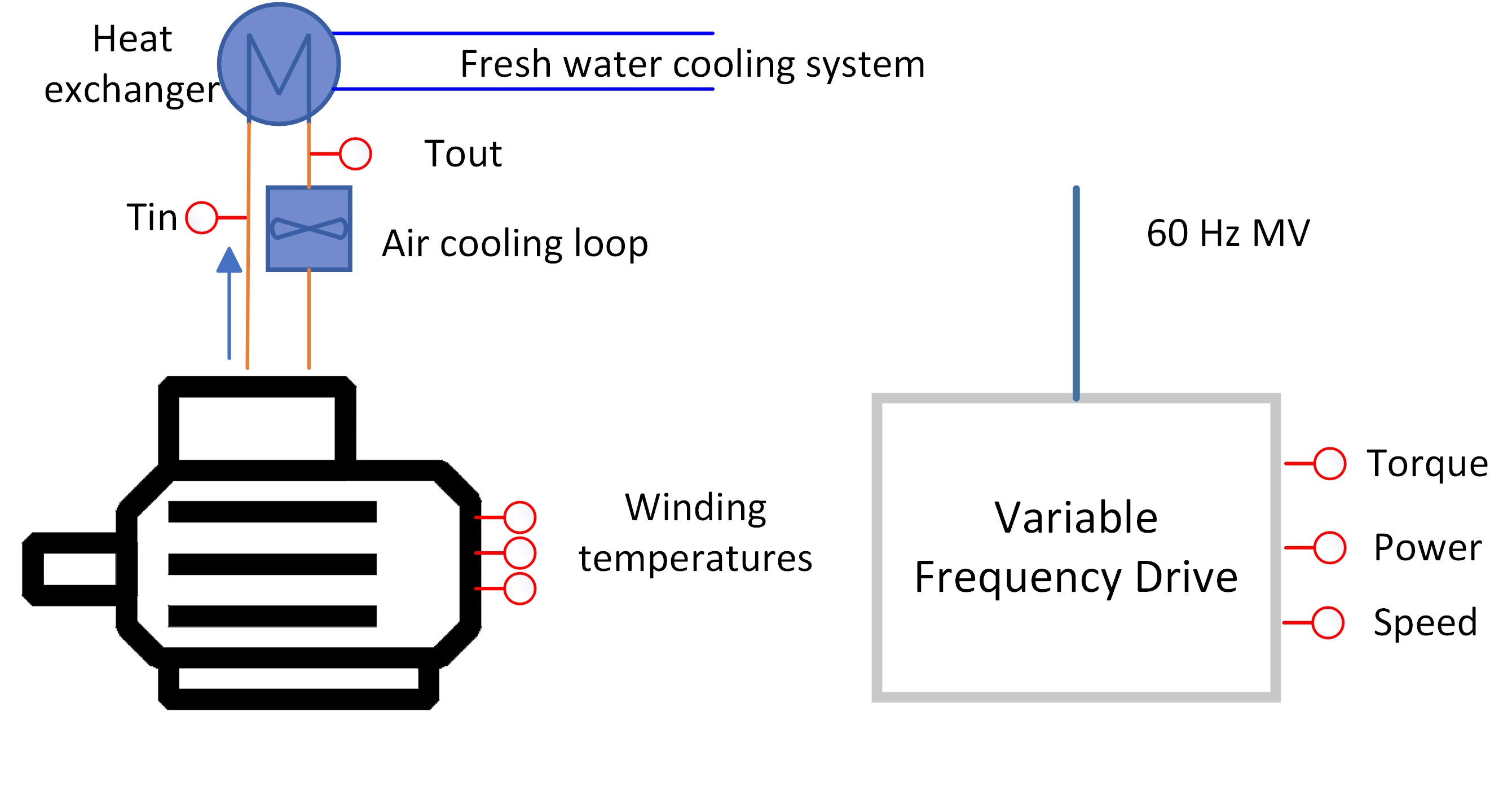
Figure 1: System overview of an electrical propulsion motor with a Variable Frequency Drive.

2.2 Dataset

Data is collected from fifteen ships with three motors each, giving a total of 45 propulsion motors. The amount of data from each motor varies, ranging from approximately one to five years, and there are 162 years of measurements in total. All measurements are collected as minute-wise averages. For each motor, the following variables are used for temperature modelling: Six stator winding temperatures, cooling air inlet temperature, power, speed, and torque. In addition, the cooling water temperature in the drive itself is used as an input, as a proxy measurement for the temperature of the fresh water cooling system.

2.3 Fault detection

Temperature sensors mounted on the stator windings are typically used to monitor overheating, see [5]. It is standard procedure to establish an alarm limit, denoted as H, and a higher trip limit, denoted as HH. When the HH limit is reached, the motor is shut down as a safety measure.

The fault detection algorithm we develop in this article is intended as a supplement to the traditional detection methods that rely on fixed limits. It provides an early warning system such that proactive measures can be taken before the motor is shut down automatically upon temperatures exceeding the HH limit.

To develop the fault detection algorithm, we follow the two-step approach of [3]:

1. Use historical data to train a machine learning model for predicting the winding temperatures from the remaining variables.

2. Monitor the difference between the observed winding temperature and predicted winding temperature on live data. When the differences become sufficiently large for a long enough time, an alarm is raised.

In the following, the difference between observed and predicted temperatures are referred to as temperature residuals.

For the fault detection algorithm to be useful, it is is essential to keep a strict control on the number of false alarms. More false alarms means a less trustworthy monitoring system and implies a high risk of alarms being ignored. Conversely, detecting the onset of an actual fault earlier provides more time to prevent catastrophic outcomes. We therefore have the following two performance requirements:

1. Minimise false alarms: The algorithm should generate as few false alarms as possible, and at least under some acceptable level.

2. Early fault detection: The algorithm should identify the beginning of actual faults as soon as possible, and at least before the HH limit is reached.

Note that from a statistical perspective, the first requirement is related to minimising the number of false positives, while the second requirement is related to minimising false negatives.

3 Concept drift

3.1 Definition and background

Concept drift is a phenomenon where the statistical properties of data changes over time in an unforeseeable way [12]. Changes in ’statistical properties’ means that the joint distribution of the data changes in some way. The drift being ’unforeseeable’ means that the drift occurs at an unexpected time and affects the joint distribution of the data in an unknown manner.

There are two sources of concept drift [12, 1]. These sources stem from dividing the entire dataset into input and output variables of a prediction model. The first source is a change in the distribution of the input variables. The second source comes from a change in the conditional distribution of the output variables given the input variables. In our setting, the second source corresponds to a change in the underlying relationship between the temperature measurements and the input variables. The result is deteriorating accuracy of the predictions. It is this source of concept drift we are primarily concerned with.

Moreover, concept drift is commonly split into four types [12, 8]: Sudden, incremental, gradual or reoccurring drift. Sudden drift means that the data distribution changes quickly from one to another. Incremental drift is the case where the data distribution changes slowly from one distribution to another. Gradual drift occurs, for example, if there are two distributional regimes, and one of the regimes are gradually observed more and more. Finally, reoccuring drift means that a previous distributional regime suddenly is reintroduced after some time. The focus of this article is on sudden drifts, as this is the type of drift observed in practice (see Section 3.2).

3.2 Concept drift in the motor data

After the initial demonstration of the performance of the fault detection procedure of [3], a project aiming to industrialise the algorithm was initiated. The goal was to deploy the algorithm to monitor the propulsion motors of an entire fleet of ships. During the final phase of retraining and onboard deployment, sudden and persistent changes in the residuals of the machine learning model were found in a large proportion of ships across the fleet. An example of an observed change in the temperature residuals is shown in Figure 2. Before the drift, the values are centered around zero, as expected, while after the drift, the values are centered around -7. The cause of the changes was later identified as a maintenance operation which modified the cooling regime in the motors. As a consequence, the performance of the fault detection algorithm was put into question.

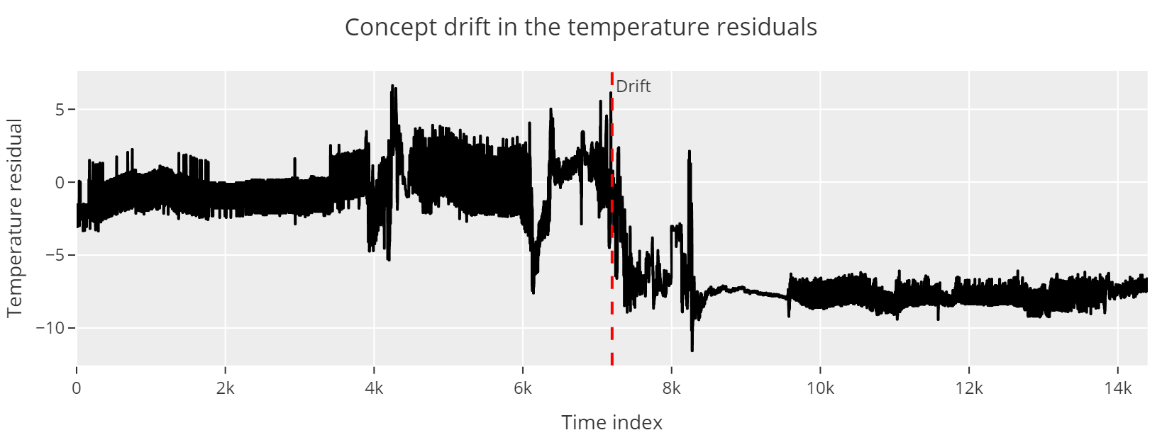
Figure 2: A real case of concept drift observed in one of the residual temperature series. After the drift, a persistent offset of around $-7$ appears in the residuals.

In this particular case, the issue could have been resolved by collecting a new training dataset, starting after the time of drift. However, the case also highlights an issue with data driven modelling, namely that the underlying system can change over time, causing models to be inaccurate. This may particularly be an issue in complex systems like a propulsion systems, which consists of an interaction of several hardware and software control systems. Potential issues that could cause a change in the system include repairs, part replacements, and software updates.

3.3 Consequences of ignoring concept drift

The following two examples highlight the effects an untreated concept drift may have in a fault detection system.

Example 1: Rise in normal temperature and increased risk of false alarms

Consider a case where the crew during maintenance replaces the fans in the cooling system with a new type, with lower rating and hence less effective cooling. This may result in a scenario where the model has been trained on data with better cooling than the current system. As a consequence, the temperature in the engine will rise, but it will not overheat (at least in our example). The performance of the model trained on the old regime, however, will start deteriorating by consistently underestimating the true temperature. Since the detection algorithm is trained on the old system, and that the new normal temperature is higher than ever observed before, it is now more likely to set off a false alarm (Figure 3).

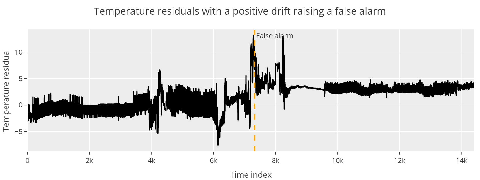
Figure 3: A rise in baseline temperature leads to a rise in the residuals which again triggers a false alarm.

Example 2: Drop in normal temperature and increased risk of blinding

In a second scenario, assume that the crew replaces the fans with a new type that has a higher rating and better cooling. This scenario exemplifies what we will call a blinding scenario. In such a case, the normal temperature decreases compared to what has been observed before, resulting in the model overestimating the true temperature. If not accounted for and a fault occurs, the alarm will be delayed, increasing the risk of missing the overheating (Figure 4).

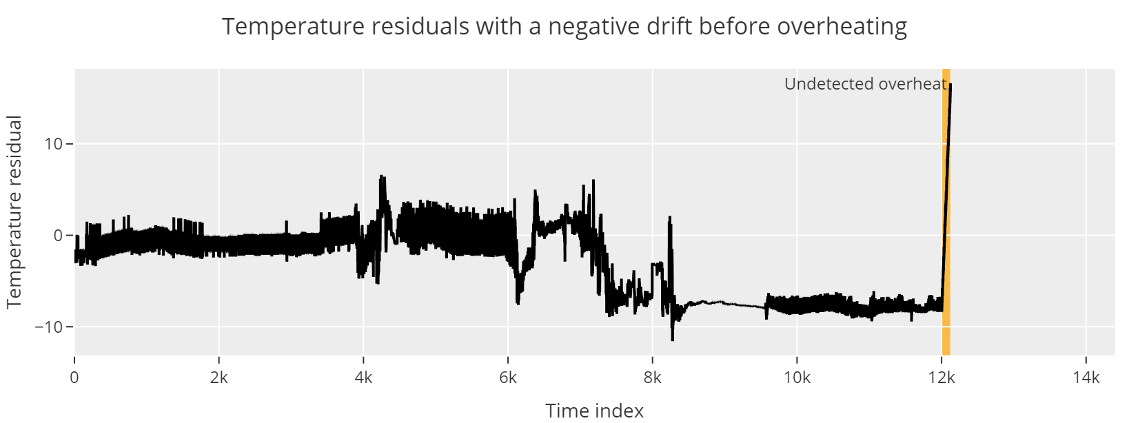
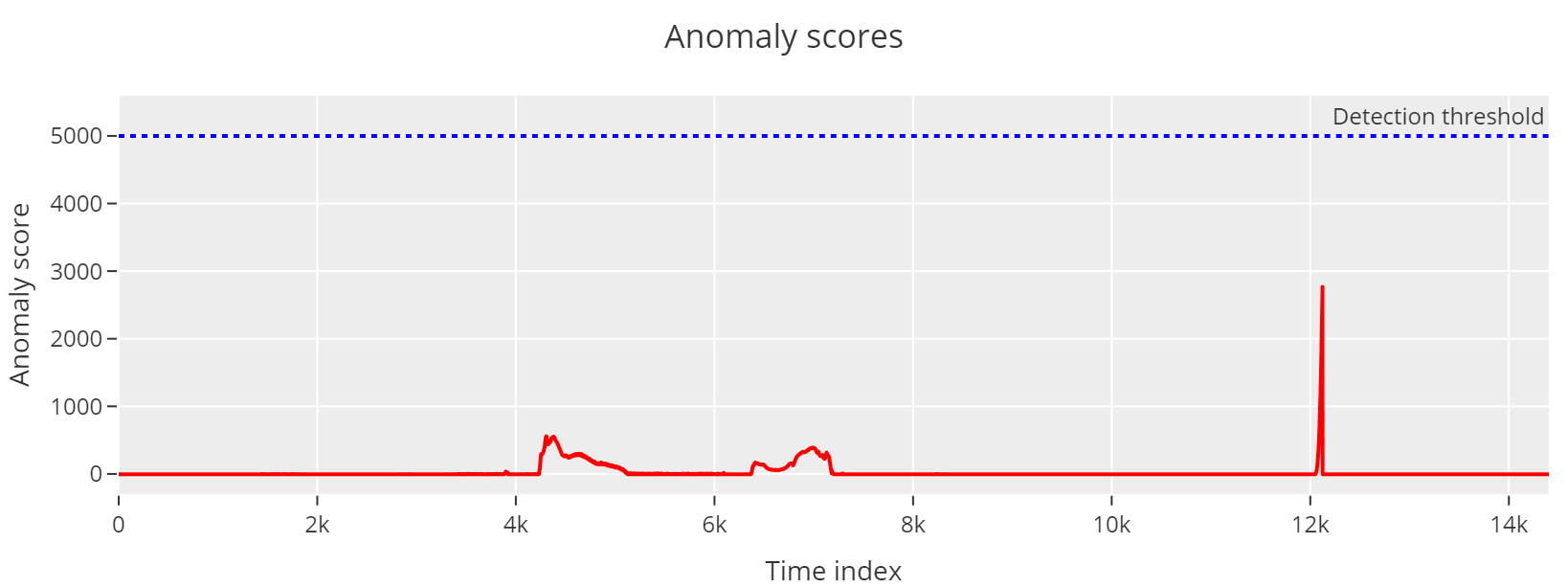
Figure 4: The baseline temperature decreases, leading to a negative bias in the residuals, masking an overheating event.

3.4 Strategies for adapting a model to concept drift

In our context, methods for dealing with concept drift can broadly be put in three different categories, described in this section.

Periodic retraining

Perhaps the simplest strategy for dealing with concept drift is to retrain the entire model at periodic intervals, say every week or every month. The model can be retrained on all available data or in a sliding window fashion. A fundamental issue with periodic retraining occurs if the model is retrained too rarely. In that case, a drift may persist untreated in the data for a sufficient amount of time for the issues described in Section 3.3 to arise. If occuring directly after a retraining, the concept drift will hence affect the system until the next retraining. Thus, it does not really solve our problem.

On-demand adaptation

Another strategy is to continuously monitor the performance of the prediction model, and retrain the model as soon as performance drops consistently by a sufficient amount. That is, a drift is first detected, then adaptation is performed when the detection demands it, thereby the name on-demand adaptation. This is the most common strategy encountered in the concept drift literature, and we develop a method of this type in Section 4.3. See [13] or [6] for examples in relation to condition monitoring. From a practical perspective, the monitoring and retraining of the model can be done in the cloud. However there is still the need to re-configure the parameters of the onboard algorithm every time a drift is detected.

Continuous adaptation

A third strategy is to continuously update the prediction model for every new sample [2]. This is known as online learning in the machine learning literature [4]. Such a strategy implicitly assumes that drifting behaviour occurs incrementally all the time, and thus skips the step of detecting whether or not a drift has occurred. It is relevant to consider this adaptation strategy, because it may be able to approximate a sudden drift by adapting sufficiently fast. We therefore present a method for continuous adaptation in Section 4.4. Considering the practical implementations of this solution, the online learning algorithm must be implemented in the ship’s on-board computation engines.

3.5 Scope

We end this section by summarising the scope of our study on simultaneous fault and drift detection.

1. Faults are characterised by large, positive change in the mean of the temperature residuals over a short time period, on the order of a few hours.

2. Drifts are also characterised by changes in the mean of the temperature residuals, but the changes are of smaller magnitude than faults, and it can change in both a positive and negative direction. In addition, drifts last for a much longer time than faults; a change is not a drift unless it lasts for more than a day. Also note that we are primarily interested in sudden drifts.

3. Known faults are extremely rare. That is, we cannot train a classifier on normal versus faulty data.

4. We are concerned with safety-critical applications, in the sense that both missed detections and false alarms are severe and should be at a very low level.

Note that distinguishing drifts and faults by their duration has been done in similar problems before, see for example [9].

4 Methods

4.1 Mathematical problem formulation

We consider the following mathematical framework for detecting faults. First, let $y_{t}=(y_{t}^{(1)},\ldots,y_{t}^{(p)})$ be the vector of the $p$ winding temperatures at time index $t$. Next, let $x_{t}$ be the vector of inputs for predicting the temperature measurements, e.g. power, speed and torque. We use the notation $x_{s:e}$ to denote the set of variables $\{x_{s},x_{s+1},\ldots,x_{e}\}$. True fault intervals are denoted by $F_{k}=(u_{k},v_{k}]$ for $k=1,\ldots,l$, where $u_{k}$ is the time of the $k$’th fault onset and $v_{k}$ is the corresponding time when the fault is a fact.

The aim is to construct a fault detector that receives the data in a streaming fashion and raises alarms only within true faults $F_{k}$ (low false alarm rate), while also detecting as many of the $F_{k}$ as possible (low missed detection rate). Formally, we define a real-time or online fault detector as a function $A_{t}:=A(x_{1:t},y_{1:t})$ that is $1$ if an alarm is raised at $t$, and $0$ otherwise. The main point of this definition is to make it clear that an alarm at time $t$ can be raised based on the entire history of the data, and not just the data observed at $t$ itself. This allows the detection of anomalous patterns in the data that are noticeable only when viewing several observations together—known as collective anomalies—and not just point anomalies. Computationally, however, the fault detector is constructed to depend on the history only through efficiently updated summary statistics over time.

The class of fault detectors we consider is based on a two stage procedure, as mentioned in Section 2.3: First, a prediction model $\hat{f}$ that generates temperature predictions $\hat{y}_{t}=\hat{f}(x_{t})$ is built on historical data. Then the temperature residuals $e_{t}=y_{t}-\hat{y}_{t}$ are monitored over time to detect overheating.

4.2 High-level algorithm

A high-level description of our fault detection method with drift adaptation is given in Algorithm 1. Notice that we first define an AdaptDrift function that takes in the temperature residuals $e_{t}$ and returns adapted temperature residuals $\tilde{e}_{t}$. Thereafter, DetectAnomaly performs anomaly detection on the adapted residuals, before the alarm times are returned.

Algorithm 1 High-level algorithm for fault detection with drift adaptation

1:Pre-trained prediction model $\hat{f}$.

2:for $t=1,2,\ldots,$ do

3:     Get temperatures $y_{t}$ and input variables $x_{t}$

4:     $\hat{y}_{t}=\hat{f}(x_{t})$

5:     $e_{t}=y_{t}-\hat{y}_{t}$

6:     $\tilde{e}_{t}=\text{AdaptDrift}(e_{t})$

7:     $A_{t}=\text{DetectAnomaly}(\tilde{e}_{t})$ $\triangleright$ $A_{t}$ is 1 if an alarm is raised, 0 otherwise.

8:$\mathcal{A}=\{t:A_{t}=1\}$ $\triangleright$ The alarm times.

Our general solution to adapting to concept drift is to use an additive drift adjustment $\hat{b}_{t}$, where $\hat{b}_{t}$ is estimated in an online manner. That is, we take

$$\text{AdaptDrift}(e_{t})=e_{t}+\hat{b}_{t},$$ (1)

in Algorithm 1. Implicitly, this means that we allow for the intercept term in the prediction method to be time-varying.

The reason for this choice of drift adaptor is that only a single parameter must be updated, rather than the entire prediction model. Moreover, it is agnostic to the choice of prediction model; it works regardless of the model being a neural network, a boosted tree model or a simple linear regression. The results (Section 5) indicate that such a drift adaptation method is adequate in the case of overheating detection for suitable choices of AdaptDrift and DetectAnomaly, discussed next.

4.3 On-demand drift adaptation

For on-demand drift adaptation of sudden concept drifts, we first run a changepoint test to test for the presence of a changepoint in the residuals. If a change is detected, then the drift adjustment $\hat{b}_{t}$ is retrained as the mean of the residuals over a period following the detection time.

A good candidate for detecting such drifts is the CUSUM (CUmulative SUM) statistic for a change in mean from zero before the change to non-zero after [14]. For a single sensor $j$, changepoint candidate $s$ and current time $t$, this CUSUM statistic is defined as

$$\mathcal{C}_{s+1:t}^{(j)}=S_{s+1:t}^{(j)}/\sqrt{t-s},$$ (2)

where $S_{s+1:t}^{(j)}=\sum_{i=s+1}^{t}e_{i}^{(j)}$. The drift score for sensor $j$ is obtained by taking the maximum over a selected set of candidate changepoints ${\mathcal{S}\subseteq\{1,\ldots,t-1\}}$:

$$\mathcal{C}_{t}^{(j)}=\max_{s\in\mathcal{S}}|\mathcal{C}_{s+1:t}^{(j)}|.$$ (3)

To get some intuition for the drift score, observe that the CUSUM statistic (2) is equal to $\sqrt{t-s}\bar{e}_{s+1:t}$, where $\bar{e}_{s+1:t}$ is the mean of the residuals since a candidate changepoint. This means that the CUSUM statistic can be large not only if the mean is large but the period $(s,t]$ is relatively short, but also if the mean is relatively small but the period is long. It reflects the idea of detecting a concept drift if it is ’sufficiently large for a sufficiently long time’, where there is an explicit trade-off between the size of the change in mean and the length of the period it is calculated over.

To get a test over all sensors, we aggregate the individual drift scores by summing them. A drift is detected as soon as the summed scores raises above a threshold $\lambda$. This gives us the global drift score

$$\mathcal{C}_{t}=\sum_{j=1}^{p}\mathcal{C}_{t}^{(j)}>\lambda,$$ (4)

Using this changepoint test statistic as our drift detector is a suitable choice due to the characteristics of the drifts we are interested in. Firstly, it uses the information that the mean of the residuals should be $0$ if the prediction model is unbiased. Secondly, it can detect both positive and negative changes in the mean of the residuals. And thirdly, it allows us to customise the candidate changepoints such that only sufficiently long periods to count as a drift may be considered.

A final feature we incorporate in the drift detector is a lag parameter $l$ in a lagged version of the CUSUM statistic, defined by

$$\mathcal{C}_{t}(l)=\mathcal{C}_{t-l}.$$ (5)

The lag parameter’s role is to avoid including observations during periods of real faults, which, in a worst-case scenario, could lead to the concept drift adaptor masking a real fault. The lag $l$ should therefore ideally be set to be larger than the longest feasible duration of an overheating event.

Regarding adapting to a detected drift, the CUSUM drift adaptor waits $n_{\text{retrain}}-l$ samples before it sets the drift adjustment $\hat{b}_{t}$ to the mean of the previous $n_{\text{retrain}}$ residuals. In other words, if drifts are detected by $\mathcal{C}_{t}(l)$ at times $\mathcal{D}=\{d_{i}\}_{i}^{q}\subseteq\{1,\ldots,t\}$, the sequence of drift adjustments becomes

$$\hat{b}_{i}=\begin{cases}0&1\leq i<d_{1}-l+n_{\text{retrain}}\\ \bar{e}_{d_{1}-l+1:d_{1}-l+n_{\text{retrain}}}&d_{1}-l+n_{\text{retrain}}\leq i<d_{2}-l+n_{\text{retrain}}\\ &\vdots\\ \bar{e}_{d_{q}-l+1:d_{q}-l+n_{\text{retrain}}}&d_{q}-l+n_{\text{retrain}}\leq i\leq t\\ \end{cases}$$ (6)

A complete summary of the CUSUM drift adaptor in a form that fits $\text{AdaptDrift}(e_{t})$ in Algorithm 1 is given in Algorithm 2. In addition, Figure 5 illustrates the behaviour of the method around the time of the real drift shown in Figure 2. Notice the discrete jump in drift adjustment as a consequence of a detected drift $n_{\text{retrain}}$ samples earlier.

Algorithm 2 CUSUM drift detection and adaptation

1:$n_{\text{retrain}}$, $\lambda$, $\mathcal{S}$

2:History of $e_{t}$ and $S_{s+1:t}$ for $s\in\mathcal{S}$, drift detection times $\mathcal{D}$, initialised as an empty set, and the previous drift adjustment $\hat{b}_{t-1}$, initialised at $0$.

3:$e_{t}$

4:$\hat{b}_{t}=\hat{b}_{t-1}$

5:$S_{s+1:t}=S_{s:t-1}+e_{t}-e_{s}$ for $s\in\mathcal{S}$.

6:if $t-\max(\mathcal{D})>n_{\text{retrain}}$ then

7:     $\mathcal{C}_{s+1:t}=S_{s+1:t}/\sqrt{t-s}$

8:     $\mathcal{C}_{t}=\sum_{j=1}^{p}\max_{s\in\mathcal{S}}|\mathcal{C}_{s+1:t}^{(j)}|$

9:     if $\mathcal{C}_{t}>\lambda$ then

10:         $\mathcal{D}=\mathcal{D}\cup\{t\}$      

11:else if $t-\max(\mathcal{D})=n_{\text{retrain}}$ then

12:     $\hat{b}_{t}=\bar{e}_{t-n_{\text{retrain}}+1:t}$

13:$\tilde{e}_{t}=e_{t}-\hat{b}_{t}$

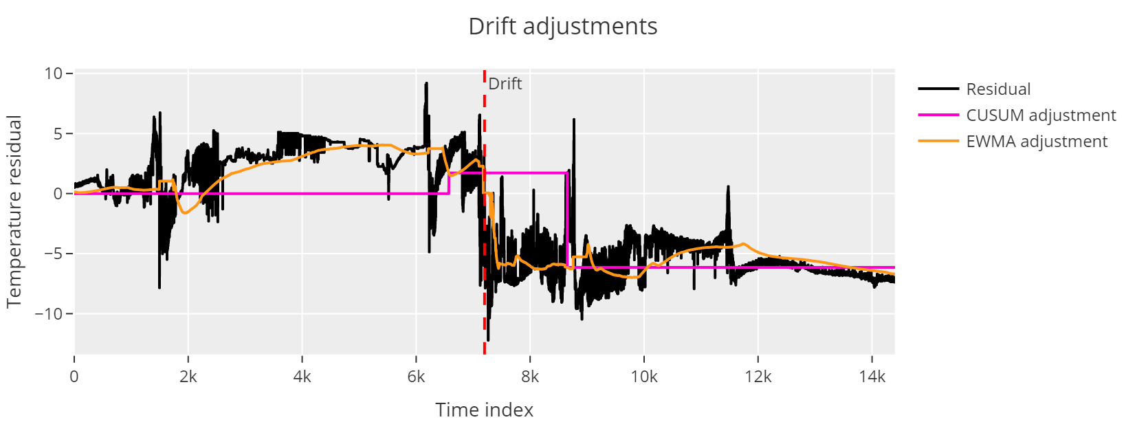
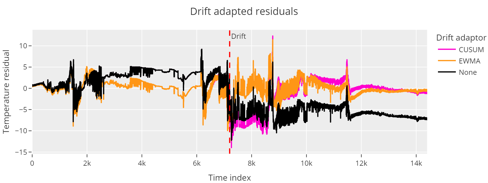
Figure 5: Drift adjustments $\hat{b}_{i}$ (top) and drift adjusted residuals $\tilde{e}_{t}=e_{t}-\hat{b}_{t}$ (bottom) for both the CUSUM and EWMA drift adaptors. Ten days of data is shown around the time of a true drift, indicated by the dashed red line. The hyper-parameters of the CUSUM and the EWMA are set to the values used in the simulation experiments described in Section 4.7.3. That is, $\mathcal{S}=\{1\text{ day},2\text{ days},\ldots,7\text{ days}\}$, $\lambda=49768$ and $n_{\text{retrain}}=400$ for the CUSUM adaptor, $\tau=8$ hours for the EWMA adaptor, and $l=4$ hours worth of samples for both.

4.4 Continuous drift adaptation

As a continuously updated drift adaptor we suggest to use a lagged Exponentially Weighted Moving Average (EWMA), given by

$$\hat{b}_{t}(\alpha,l)=(1-\alpha)\hat{b}_{t-l-1}+\alpha e_{t-l}.$$ (7)

To set the decay parameter $\alpha$, we parameterise it by its half-life $\tau$, meaning the number of samples it takes for the value of $e_{t-l}$ to be reduced to half its value. This gives us $\alpha=(1/2)^{1/\tau}$. The lag paramter $l$’s role is the same as for the CUSUM method: To avoid masking real faults.

See Figure 5 for an illustration of how the EWMA adaptor behaves compared to the CUSUM method. Notice the smooth adaptation compared to the discrete jumps of the CUSUM method.

4.5 Detecting anomalous sequences of residuals

In this section we briefly describe the algorithm for detecting anomalies in the residuals developed by [3], and fit it within the fault detection framework of Section 4.1 and DetectAnomaly of Algorithm 1.

The mentioned algorithm is a sequential changepoint detection method for detecting consistently large positive deviations in a data sequence, originally due to [11] and [10]. It requires two hyper-parameters to be set: A detection threshold $\gamma$ and a smallest relevant size of the change in mean $\rho$. Like for the drift detector in Section 4.3, the top level of the algorithm consists of aggregating per-sensor scores, but this time the maximum is used as aggregator to retain sensitivity to potential hotspots forming in the motor. Thus, the global anomaly score is given by

$$G_{t}=\max_{j=1,\ldots p}z_{t}^{(j)},$$ (8)

where $z_{t}^{(j)}$ are per-sensor scores given by the adaptive recursive CUSUMs,

$$z_{t}^{(j)}=\max\left(z_{t-1}^{(j)}+\hat{\mu}_{t,j}\tilde{e}_{t}^{(j)}-\frac{1}{2}\hat{\mu}_{t,j}^{2},0\right).$$ (9)

Further, the mean estimates $\hat{\mu}_{t,j}$ are updated as running means from the most recent time $z_{t}^{(j)}=0$, but bounded below at $\rho$. It is calculated as follows:

$$\hat{\mu}_{j,t}=\max\left(\frac{s_{j,t}}{n_{j,t}},\rho\right),\quad s_{j,t}=\begin{cases}s_{j,t-1}+\tilde{e}_{j,t-1},&z_{j,t-1}>0,\\ 0,&z_{j,t-1}=0,\end{cases}$$ (10)

where $n_{j,t}=n_{j,t-1}+1$, if $z_{j,t-1}>0$, and otherwise $n_{j,t}=0$, if $z_{j,t-1}=0$, and with initial values $z_{j,0}=s_{j,0}=\tilde{e}_{j,0}=0$. When $s_{j,t}=n_{j,t}=0$, we set $s_{j,t}/n_{j,t}=0$. Finally, an alarm is raised as soon as $G_{t}>\gamma$. Please see [3, Section 3.2.1] for a more thorough discussion and intuition behind the method.

To fit the adaptive CUSUM into DetectAnomaly in Algorithm 1, we need a resetting mechanism upon an alarm being raised. So far, $G_{t}$ is only equipped to run until a single alarm is raised, while a fault detector as we have defined it, should be able to generate several alarms. We propose the following resetting mechanism: If an alarm is raised at $a_{i}$, we reset the detector, and wait $R>0$ samples before it starts running again. We refer to $R$ as the restart delay. Thus, if letting $r_{i}=a_{i}+R$ be the reset time corresponding to alarm $a_{i}$, and $r_{0}=0$, the alarm times are given by

$$a_{i}=\inf\left\{t>r_{i-1}:G_{t}>\gamma\right\},\quad i=1,\ldots,m.$$ (11)

$\text{DetectAnomaly}(\tilde{e}_{t})$ is $1$ on the times $a_{i}$, and $0$ otherwise.

4.6 Tuning the change detectors

To set the CUSUM drift detection threshold $\lambda$ and the anomaly detection threshold $\gamma$ we use a data driven procedure that relates the choice of threshold to an approximate number of acceptable false detections, $q_{\text{val}}$. It is important that this procedure is run on a separate validation dataset different from the data used to train the prediction model. In this way, the residuals are based on out-of-sample predictions like in a real monitoring setting. Moreover, it is best if the validation or tuning dataset does not contain drifts or faults, as $q_{\text{val}}$ will not reflect the amount of false positives anymore. If the data contains $k$ drifts or faults, however, the tuning procedure nonetheless offers robustness against learning these events as being normal by setting $q_{\text{val}}>k$.

For the CUSUM drift detection score $\mathcal{C}_{t}$, the steps are as follows:

1. Run the detector over the residuals from the validation set to get $\mathcal{C}_{1:t}$ over the whole set.

2. Start with $\mathcal{T}=\{1,\ldots,t\}$, then iteratively, for $q_{\text{val}}$ iterations, find $\max_{t\in\mathcal{T}}\mathcal{C}_{t}$ and remove a period around $\tau=\text{argmax}_{t\in\mathcal{T}}\mathcal{C}_{t}$ from $\mathcal{T}$. We choose to remove such a period by stepping to the left and right of $\tau$ until the value of $\mathcal{C}$ is below a threshold in either direction. We set the threshold to the 0.2-quantile of the distribution of $\mathcal{C}_{1:t}$.

3. The value of $\max_{t\in\mathcal{T}}\mathcal{C}_{t}$ from the last iteration is the tuned threshold at $q_{\text{val}}$ acceptable false alarms in the drift-free validation data.

The procedure can be adapted to the anomaly detection score by exchanging $\mathcal{C}_{t}$ with $G_{t}$.

4.7 Performance assessment

In this section we turn to the details of how we analyse the motor data and assess the performance of the proposed concept drift adaptation methods.

4.7.1 Training, validation and testing pipeline

Two months before the time of drift and onwards into the future is taken as the test set for each ship. If there is no concept drift on a ship, we use the last 25% of samples as the test set instead. The remaining, pre-drift data is split equally between training and validation sets, where the first half is the training set, and the latter half is the validation set. This split resulted in 29.3% training, 29.3% validation and 41.4% testing observations overall, but with large variations from motor to motor.

On a high level, the pipeline for training, tuning and testing is given by the following steps:

1. Train a prediction model on the training set.

2. Tune the anomaly and drift detectors on the residuals of the predictions in the validation set.

3. Run the fault detector with drift adaptation (Algorithm 1) on the test set.

4.7.2 Prediction model training

As our prediction model for the motor temperature, we train one boosted tree model with squared error loss per motor. The HistGradientBoostingRegressor of Scikit-learn [15] is used to fit the model. The maximum tree depth, the number of iterations and the learning rate were tuned by five-fold cross-validation. The full list of input features to the prediction model is:

1. Power and EWMA-transformed power with a 30 minute half-life.

2. Speed and EWMA-transformed speed with a 30 minute half-life.

3. Torque and EWMA-transformed torque with a 30 minute half-life.

4. Air inlet cooling temperature.

5. Water cooling unit temperature.

6. The time since the motor was last turned on or off.

7. How long time the motor was in the on or off state previous to the current state.

8. An indicator for each sensor.

See [3] for a thorough dicussion on the input variables.

4.7.3 Drift and anomaly detector parameter settings

Based on prior knowledge about the characteristics of faults and drifts (Section 3.5), we have used the following parameter settings.

• CUSUM drift adaptor: The number of retraining samples $n_{\text{retrain}}=400$ (approximately $6.7$ hours), lag $l=4$ hours and candidate changepoint set $\mathcal{S}=\{1\text{ day},2\text{ days},\ldots,7\text{ days}\}$. $\lambda$ is set according to the tuning procedure described in Section 4.6 such that $q_{\text{val}}=200$ across the validation data of all motors.

• EWMA drift adaptor: Half-life $\tau=8$ hours and lag $l=4$ hours worth of samples.

• Anomaly detector: Minimum change size $\rho=30$ and reset delay $R=4$ hours. $\gamma$ is varied to obtain the missed detection versus false alarm curves (see Section 4.7.5).

4.7.4 Fault simulation

Overheating events are extremely rare, so we choose to simulate faults to obtain a sufficient span of different fault scenarios. Simulated faults are characterized by their onset time $u_{k}$, which sensors $\mathcal{J}\in\{1,\ldots,p\}$ are affected, and a slope parameter $a$ governing how quickly the temperature rises. For a fixed onset time, faults are injected in the data by adjusting the temperature measurements by $y_{t,j}=y_{t,j}+a(t-u_{k})$ until $\max_{j}y_{t,j}$ reaches a temperature of 145, for $t>u_{k}$ and $j\in\mathcal{J}$. The maximum temperature of 145 represents a temperature threshold where the motor would be tripped by the fixed alarm, and the time it occurs is the end point of $F_{k}$.

4.7.5 Experimental setup

The purpose of the experiment is to observe how drift adaptation affects fault detection performance. We consider nine scenarios in total: Negative drift, positive drift and no drift, as well as overheating slopes $a=0.5,1,1.5$ for each of the drift scenarios. The steeper the slope, the harder it is to detect the overheating in time. For each scenario, we run the fault detector with the CUSUM drift adaptor, the EWMA drift adaptor, and without any drift adaptor. The anomaly detection threshold $\gamma$ is varied to get missed detection rate versus false alarm rate curves for each method.

The negative drift scenario is the real, observed drift cases in the data, where all the drifts result in decreased baseline motor temperature. As the direction of drift influences the fault detection performance in fundamentally different ways, we have also added a scenario where the direction of drift has been ’flipped’ from a negative to a positive direction. That is, we have calculate the the difference in mean temperature before and after each drift, and flip the sign of the change to get the positive drift scenario. To get the no drift scenario, we use the same procedure to remove the real drift.

For each of the drift and fault scenarios, 1000 simulated overheating events are injected in the test set, distributed evenly across the motors. Representing a worst-case scenario, only one sensor is affected in each simulated fault. The faulted sensor is selected at random. The onset times are drawn uniformly from all timestamps, but restricted such that two faults are separated by a minimum of 12 hours of non-faulty observations. Moreover, to represent motor shut-down upon detection of a simulated fault, the drift adapted residuals are set to zero for the next six hours.

4.7.6 Performance evaluation

We record an alarm as a true positive if it is raised within any of the fault intervals $\cup_{k=1}^{l}F_{k}$ and a false positive otherwise. A false negative or missed detection occurs if a fault interval $F_{k}$ does not contain any alarms. Denote the total number of false positives, true positives and false negatives across all the ships by $FP$ and $FN$, respectively. Moreover, let $P=1000$ be the total number of faults and $T=67$ be the total length in years of testing data across all motors. From these fundamental quantities, we obtain the missed detection rate as $FN/P$ and an average false alarm rate per motor and year as $FP/T$.

5 Results

The missed detection rate versus the average false alarm rate per motor per year for the different drift and fault scenarios is shown in Figure 6. Recall that $\gamma$ is varied to obtain the relationship between the false alarm and missed detection rate. A missed detection rate close to 1.0 is of no operational value. Hence, when comparing the performance of different drift adaptors, the lower region (missed detection rate $\leq 0.01$) of each subplot is the most important. In addition, we consider a false alarm rate less than $1.0$ per motor per year acceptable.

There are several interesting observations to be made in the figure: First, observe that the EWMA method (pink lines) is the best method in all the scenarios In addition, it always has less than the acceptable $1.0$ false alarm rate. Second, notice that the CUSUM method (orange lines) performs slightly worse than the EWMA method, with a more or less constant difference in performance across all the scenarios. It also fulfills the false alarm rate requirement of less than $1.0$ in all scenarios, though, except for positive drifts with less than $0.001$ missed detection rate. Third, when comparing the results for handling (the coloured lines) versus not handling concept drift, the greatest improvement in performance is seen for positive drifts, where the drift adaptors have a false alarm rate of less than a tenth compared to not handling the drift. For the negative drifts observed in our dataset, on the other hand, it is beneficial to not adapt to the drift rather than using the CUSUM method, and using the EWMA method is only slightly better. Finally, as expected, the performance of all the methods decrease as the overheating slope gets steeper (moving from left to right in the figure), although the difference is not great.

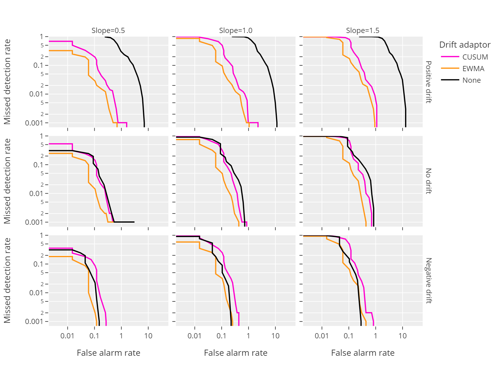
Figure 6: Missed detection rate versus average false alarm rate per motor per year for each of the combinations of drift and fault scenarios.

6 Discussion

This article presents a solution for dealing with concept drifts in fault detection systems based on monitoring residuals from a prediction model. The solution applies an additive adjustment term to the residuals, rather than retraining the entire model. This allows for easily understandable, quick and on-the-fly adaptation of drifts, eliminating fault monitoring downtime due to retraining. An underlying assumption of the solution is that faults occur over shorter time-spans than concept drifts.

We have concentrated on concept drifts that result in sudden changes in the mean of the residuals. Given that the space of possible concept drifts is infinite, this is a limiting factor. However, the observed drifts in the motor data were all of this type, so the methods solve the problem at hand. Dealing with more complicated drifts is left for future work, until the data demands it.

The results from the data analysis show that drift adaptation is beneficial for fault detection performance in the motor data, especially for the EWMA method. The reason why the EWMA method also performs better in the cases with no drift (the middle row of Figure 6), is that the prediction model is not perfect, such that the residuals have a slowly varying trend, without it being a concept drift. This is visible in the period before the known concept drift in Figure 5, where the residuals consistently lie around values of 3-4 for a few days. The EWMA method will automatically adapt also to these imperfections. The CUSUM method with the tuning parameters we have selected, on the other hand, only deems the largest of these fluctuations as severe enough to adapt to (which happens just before the real concept drift in Figure 5).

The results also show that negative drifts of the sizes observed in our data does not benefit much from drift adaptation; the EWMA method performs a little better, while the CUSUM method performs worse than not adapting to the drift. There are two reasons for this. The first is that a negative drift not only masks true positives if not dealt with (Figure 4), it also protects against false positives. The second is that the drifts in the data are relatively small in size compared to the large overheating deviations, such that the overheating events are detected despite the negative drift. Negative drifts of higher magnitudes would likely influence the missed detection rate of not taking concept drift into account more severely.

In our analysis, we have simulated faults by a linearly increasing trend until a limit temperature is reached. This is a simplification of how real overheating events would look, but it captures its main characteristic, namely an increasing temperature. Since the point of the analysis is to compare the different drift adaptors and no drift adaptation with each other under equal and easy to understand circumstances, our method of simulating faults are sufficiently representative of real faults. If the point had been to create as accurate and realistic false alarm and missed detection rates as possible, we would have to use other methods.

For an algorithm that performs adaption to concept drift, a worst case scenario is that the model adapts to a fault such that it is masked. As presented in Section 4.4, a safeguard is included in both the CUSUM and the EWMA method, by introducing a lag in the estimation of the drift adjustment term. Putting additional constraints or limits on this adjustment term is a straight forward extension. It should be noted that the H alarm limit and HH trip limit will stay in place, such that the conventional protection still works.

Finally, we have seen that there is a fundamental issue with fault detection algorithms based on monitoring residuals from a prediction model. You can never be completely certain whether the residual is large due to the measurements, as desired, or due to a poor model. Thus, in future work, it will be interesting to explore other kinds of fault or anomaly detection techniques, not based on residuals.

Declaration of interests

The authors have nothing to declare.

References

- [1] João Gama et al. “A survey on concept drift adaptation” In ACM Computing Surveys 46.4, 2014, pp. 44:1–44:37 DOI: 10.1145/2523813
- [2] Wolfgang Grote-Ramm et al. “Continual learning for neural regression networks to cope with concept drift in industrial processes using convex optimisation” In Engineering Applications of Artificial Intelligence 120, 2023, pp. 105927 DOI: 10.1016/j.engappai.2023.105927
- [3] K.. Hellton et al. “Real-time prediction of propulsion motor overheating using machine learning” Publisher: Taylor & Francis _eprint: https://doi.org/10.1080/20464177.2021.1978745 In Journal of Marine Engineering & Technology 21.6, 2021, pp. 334–342 DOI: 10.1080/20464177.2021.1978745
- [4] Steven C.. Hoi, Doyen Sahoo, Jing Lu and Peilin Zhao “Online learning: A comprehensive survey” In Neurocomputing 459, 2021, pp. 249–289 DOI: 10.1016/j.neucom.2021.04.112
- [5] “IEEE Recommended Practice for Motor Protection in Industrial and Commercial Power Systems” Conference Name: IEEE Std 3004.8-2016 In IEEE Std 3004.8-2016, 2017, pp. 1–163 DOI: 10.1109/IEEESTD.2017.7930540
- [6] Nicolas Jourdan, Tom Bayer, Tobias Biegel and Joachim Metternich “Handling concept drift in deep learning applications for process monitoring” In Procedia CIRP 120, 56th CIRP International Conference on Manufacturing Systems 2023, 2023, pp. 33–38 DOI: 10.1016/j.procir.2023.08.007
- [7] Çağlar Karatuğ, Yasin Arslanoğlu and C. Soares “Review of maintenance strategies for ship machinery systems” Publisher: Taylor & Francis _eprint: https://doi.org/10.1080/20464177.2023.2180831 In Journal of Marine Engineering & Technology 22.5, 2023, pp. 233–247 DOI: 10.1080/20464177.2023.2180831
- [8] Marília Lima, Manoel Neto, Telmo Silva Filho and Roberta A. A. “Learning Under Concept Drift for Regression—A Systematic Literature Review” Conference Name: IEEE Access In IEEE Access 10, 2022, pp. 45410–45429 DOI: 10.1109/ACCESS.2022.3169785
- [9] Jiayi Liu et al. “Anomaly and change point detection for time series with concept drift” In World Wide Web, 2023 DOI: 10.1007/s11280-023-01181-z
- [10] Kun Liu, Ruizhi Zhang and Yajun Mei “Scalable SUM-Shrinkage Schemes for Distributed Monitoring Large-Scale Data Streams” In Statistica Sinica 29, 2017, pp. 1–22 DOI: 10.5705/ss.202015.0316
- [11] Gary Lorden and Moshe Pollak “Sequential Change-Point Detection Procedures That are Nearly Optimal and Computationally Simple” In Sequential Analysis 27.4, 2008, pp. 476–512 DOI: 10.1080/07474940802446244
- [12] Jie Lu et al. “Learning under Concept Drift: A Review” In IEEE Transactions on Knowledge and Data Engineering 31.12, 2019, pp. 2346–2363 DOI: 10.1109/TKDE.2018.2876857
- [13] Minghua Ma et al. “Robust and Rapid Adaption for Concept Drift in Software System Anomaly Detection” ISSN: 2332-6549 In 2018 IEEE 29th International Symposium on Software Reliability Engineering (ISSRE), 2018, pp. 13–24 DOI: 10.1109/ISSRE.2018.00013
- [14] Ewan S. Page “Continuous inspection schemes” In Biometrika 41.1, 1954, pp. 100–115 URL: http://www.jstor.org/stable/2333009
- [15] Fabian Pedregosa et al. “Scikit-learn: Machine Learning in Python” In Journal of Machine Learning Research 12, 2011, pp. 2825–2830 DOI: 10.48550/arXiv.1201.0490
- [16] Christian Velasco-Gallego et al. “Recent advancements in data-driven methodologies for the fault diagnosis and prognosis of marine systems: A systematic review” In Ocean Engineering 284, 2023, pp. 115277 DOI: 10.1016/j.oceaneng.2023.115277