Effective Polaron Dynamics of an Impurity Particle Interacting with a Fermi Gas
Abstract
We study the quantum dynamics of a homogeneous ideal Fermi gas coupled to an impurity particle on a three-dimensional box with periodic boundary condition. For large Fermi momentum , we prove that the effective dynamics is generated by a Fröhlich-type polaron Hamiltonian, which linearly couples the impurity particle to an almost-bosonic excitation field. Moreover, we prove that the effective dynamics can be approximated by an explicit coupled coherent state. Our method is applicable to two relevant settings: first, an interaction coupling and masses of order 1 for time scales of order ; second to the case of and a heavy Fermi gas with masses of order for time scales of order 1.
Abstract
1 Introduction
The study of impurities in quantum gases has garnered considerable attention due to its relevance in various physical contexts, ranging from solid-state physics to cold atom experiments. In this context quasi-particles such as polarons stand as intriguing entities emerging from the interaction of a single impurity particle with a surrounding medium. The concept of a polaron, originally introduced by Lev Landau to study the motion of an electron in a dielectric crystal [1965], most famously emerges from the celebrated Fröhlich Hamiltonian in second quantization formalism describing electron-phonon interactions [Froehlich1954]. Subsequently, the polaron concept was extended to all kind of surrounding media including Bose and Fermi gases. The formation conditions and properties of polarons are believed to play a central role to understand the transport properties and the effective mass of impurities within the host material.
In this article, we study with mathematical rigor the dynamics of an impurity particle immersed in a dense gas of fermions as surrounding medium. Interactions between fermions are neglected and we assume that the initial state of the system is a product state between the impurity state and a filled Fermi ball. This mathematical framework finds resonance with recent experimental and theoretical advancements in the study of ultracold atoms [SWSZ09, KSN+12, CJL+15]. We show that the effective dynamics of the system is governed by a Fröhlich-type Hamiltonian, which linearly couples the impurity particle to an almost-bosonic excitation field. More specifically, the excitations relative to the filled Fermi ball are up to a constant described by the Hamiltonian
| (1.1) |
with describing the kinetic energy of the impurity
particle, describing the kinetic energy of
the excitation field and
the linear coupling between impurity particle and excitations. The
operators and describing this excitation field coincide
with those introduced in a series of pioneering studies on the correlation
energy of interacting fermions [BNP+19, BNP+21a, BNP+21b].
We note that an effective Hamiltonian of a similar type to (1.1)
has recently been derived in another microscopic setting involving
a tracer particle interacting with excitations of a Bose Einstein
condensate [LP22, MS20].
Subsequently, we show that the effective time evolved state can be
up to a phase factor approximated by a time-dependent coupled coherent
state where is the Weyl operator
which is simply parameterized by a function . An explicit
expression for is derived which allows for determining
the number of collective excitations over time. We believe that such
quantities are in particularly helpful to gain deeper insights into
the formation process of quasi-particles as studied in experiments
such as [CJL+16]. Eventually, we show that the linear coupling
term cannot be omitted in the effective description
but adds a leading order effect to the effective dynamics in our setting.
Our results hold for a variety of time scales and couplings, describing different interaction strengths and mass ratio, which will be specified in the subsequent section. We note that the same microscopic model has been studied in [JMPP17, JMP18, MP21] but with very specific choices of couplings different from ours, leading to an effective decoupling of impurity and gas.
1.1 The microscopic model
We consider an impurity particle interacting with spinless fermions on a 3-dimensional box with periodic boundaries described by . The system is described by a state in the Hilbert space with where is the coordinate of the impurity particle and are the coordinates of the fermions. The Hamiltonian of the system is given by
| (1.2) |
and parameterized by the coupling constants . Note that the different parts of the Hamiltonian on different tensor components of our Hilbert space writing, i.e. we used the short-hand notation writing, for example, for the Laplacian acting on the impurity particle. The interaction is assumed to have a Fourier transform with compact support satisfying for all . It is well-known that under this assumption the Hamiltonian (1.2) defines a self-adjoint operator which generates by Stone’s theorem the unitary time evolution .
We are interested in the dynamics of the system governed by the time-dependent Schrödinger equation of the form
| (1.3) |
Note that the ground state of the non-interacting Fermion system is well-known, non-degenerate and explicitly given by
| (1.4) |
We choose the initial state to be of product form
| (1.5) |
with a general state for the impurity particle i.e. the system is initially prepared in a state describing the ground state of the ideal Fermi gas which does not interact with the impurity particle.
Furthermore, we choose the Fermi momentum to be our parameter of the system in the sense that the particle number is defined as
| (1.6) |
i.e. the particle number of the Fermi gas is chosen such that the Fermi ball is completely filled. Note that the average density is in this case proportional to the number of gas particles due to the following relation
| (1.7) |
which is a consequence of Gauss’ counting algorithm.
1.2 Scaling regimes
In the following, we present the choices of and we are aiming for, and discuss the physical meaning of the couplings.
-
•
The coupling models the coupling strength between the Fermi gas and the impurity. For small we expect a decoupling between the gas and the impurity in the sense that the time evolution given by (1.3) does not entangle an initial state of product form . Such a result was shown in [MP21] with and in three dimensions and [JMPP17, JMP18] with in two dimensions.
-
•
The couplings and determine the order of the kinetic energy of the impurity and Fermi gas respectively.
-
•
In addition, it is important to discuss on which time scales results hold. Define to be the relevant time scale for our statements, i.e. our statements shall be considered for with .
Our results hold for the following set of couplings
| (1.8) |
The physical interpretation can be better understood in the following specific cases:
Fermi time dynamics , with ,
In this setting the kinetic energy of the Fermi gas and the interaction term are chosen independent of the the Fermi momentum and, in particular of the particle number . In return the considered time scale is and therefore short for large . Planck’s constant is set to be , the Fermion mass is of order 1. For convenience we set in this case. The mass of the impurity particle might depend on and represent for and large a light, for a heavy or for an equally heavy impurity particle in comparison to the fermions. We remark that the results in [MP21] can be transferred to this setting of , however, allowing only for shorter timescales of for a . This seems compatible since we are not interested in a free time evolution of the impurity particle. The times are on the time scale of the fermions near the Fermi surface, which typically have a momentum of .
Heavy fermion regime , with ,
In this setting, we identify the couplings and with the masses of the fermions and the impurity particle, respectively. More concretely, the fermion mass is and the mass of the impurity particle is where the factor is chosen for convenience. Since we are interested in large , this case corresponds to a heavy Fermi gas setting where the impurity particle has a relative mass ratio of depending on . The coupling strength between both impurity particle and gas is weak but much stronger than in the mean-field setting where one would introduce an averaging factor of . Planck’s constant is set to be in this case and is particularly independent of the number of gas particles.
Semiclassical regime , with ,
We can also identify the couplings with Planck’s constant instead of setting it to . In this case, we consider the time evolution governed by the Schrödinger equation
| (1.9) |
with . The fermion mass is given by and mass of the impurity particle with . The time evolution is therefore given by the operator . Since the time scale is absorbed by the factor is of order .111Note that the effective Hamiltonian is expected to be of order here such that the exponent of the time evolution operator is of order . Since we are interested in , the interpretation is that the system is considered in the semiclassical regime with . Such a semi-classical regime with has been widely studied in the analysis of Fermi gases, as can be seen for example in [Ben22, Saf23].
From a technical point of view all settings are very similar and our results will apply to all described cases. We will focus our presentation on the setting with and give some remarks how the results can be translated to the semiclassical setting.
2 Preliminaries
2.1 Second quantization
It is convenient to consider as -particle sector of with the fermionic Fock space constructed over . This way, we have access to the powerful formalism of second quantization with the fermionic creation operator creating a particle with momentum and the annihilation operator annihilating a particle with momentum . Those operators satisfy the canonical anticommutation relations (CAR)
| (2.1) |
Furthermore we introduce the fermionic number operator and the vacuum satisfying for all .
We lift our -particle Hamiltonian to Fock space as
| (2.2) |
which agrees to if restricted to . We denote by the inner product on and by the induced norm if not stated otherwise.
We will mostly use the abuse of notation as operator on where acts as an operator on the Fock space part.
2.2 Particle-hole transformation
In our analysis, a primary objective is to focus on excitations relative to the non-interacting Fermi ball. In particular, we want to use a description of our fermionic system in which the non-interacting Fermi ball is mapped to the vacuum. To achieve this, we employ the particle-hole transformation, which is a specific type of fermionic Bogoliubov transformation as creation operators are mapped to linear combinations of creation and annihilation operators while preserving the CAR. The particle-hole transformation is defined as the map satisfying
| (2.3) |
It is easy to check that the map is well-defined, unitary and satisfies .
With this, we can re-write the initial state (1.5) representing a non-interacting impurity particle and a Fermi gas as
| (2.4) |
Later on, we will mostly use the product state
of the impurity and the vacuum instead of .
Furthermore, we define
| (2.5) |
to be the energy of the non-interacting Fermi ball.
Of greatest interest is of course the action of the particle-hole transformation on the microscopic Hamiltonian as generator of the dynamics. The conjugation with of yields
| (2.6) | ||||
| (2.7) | ||||
| (2.8) |
Similarly, we can see that
| (2.9a) | ||||
| (2.9b) | ||||
For later purposes we shall introduce for the short-notation
| (2.10) | ||||
| (2.11) |
We can then write
| (2.12) |
with and is given by the terms of (2.9b) since
| (2.13) |
where we used that .
2.3 Almost-bosonic operators and patch decomposition
Our effective description of the microscopic system described by (1.2) will involve the emergence of almost-bosonic particles describing pair excitations of the Fermi ball. Those pair excitations will be delocalized over the Fermi surface in the sense that they correspond to a linear combination of two fermionic creation operators. As mentioned before the almost-bosonic pair operators which occur in this article coincide with the ones introduced in the series of seminal works [BNP+19, BNP+21a, BNP+21b, BPSS23] on the correlation energy of a weakly interacting Fermi gas. We give a brief introduction to the construction of those operators with the most relevant properties in the this subsection and in Section A.
A key ingredient for the approximation of the microscopic fermionic system by almost-bosonic excitations is the decomposition of the Fermi surface into patches. This will allow to approximate the fermionic kinetic energy term by a term quadratic in the almost-bosonic pair operators.
Introduce the bisecting subset of
| (2.14) |
allowing the decomposition .
The construction works as follows:
-
(i).
Choose the number of patches satisfying
(2.15) Equivalently, we can also write the condition as with and ). The lower bound on is needed to control the number of momenta inside each patch whereas the upper bound is needed to suppress Pauli’s principle. The choice of and will be taken later.
-
(ii).
Define equal-area disjoint patches centered around as follows
-
•
is spherical cap of area ,
-
•
decompose remaining semi-sphere into collars,
-
•
leave corridors of width between adjacent patches,
-
•
define patches of southern semi-sphere by reflection .
-
•
-
(iii).
For given define the index set consisting of north and south patch indices
(2.16) (2.17) A thin strip around the equator has to be excluded since the number of momenta per equator patch is too small. Note that coincides with the parameter in step 1.
-
(iv).
Define the collective almost-bosonic creation operator and its normalization factor as
(2.18) with
(2.19) being sensitive to being on the north or south hemisphere. The creation operator can be seen as collective in the sense that it involves a superposition of all possible fermion pairs with relative momentum .
Similarly to (2.11) introduced in the previous subsection, we define
| (2.20) |
with inner product for all .
The following statements hold as a consequence of the above construction.
-
•
The surface area of a patch satisfies .
-
•
The Canonical Anticommutation Relations (CAR) are satisfied up to an error term (see [BNP+19, Lemma 4.1]): It holds for all and
(2.21) (2.22) satisfying , and
(2.23) -
•
The almost-bosonic operators change the number operator by two (see [BNP+19, Lemma 2.3]) in the following sense
(2.24) -
•
The normalization constant satisfies (see [BNP+19, Proposition 3.1])
(2.25)
Also note that the summation in the definition of the almost-bosonic operators and involves only finite sets. Unlike in the exactly bosonic case our almost-bosonic operators therefore inherit boundedness from the fermionic constituents which satisfy . Subtle questions about the self-adjointness and domain of the almost-bosonic operators remain trivial in our case.
2.4 Almost-bosonic coherent state
Since defines for all a bounded operator and satisfies , the exponential operator is well-defined and is unitary.
Definition 2.1.
Define for the Weyl operator
| (2.26) |
If is additionally a bounded multiplication operator for each , we call a coupled coherent state with .
Remark 2.2.
If would satisfy the CCR without error, one could use the Baker-Campbell-Hausdorff formula to formally write
| (2.27) |
i.e. the coupled coherent state corresponds to a superposition of different particle number. Later on , the terms and with the function will take the role of interaction term with an multiplication operator acting on . Thus the occurrence of in each component of the vector representation stresses the coupling between the function and the bosonic -particle state via the interaction .
In the following we show that well-known properties of the Weyl operator (cf. for example [BPS16, Chapter 3] or [FZ17, Appendix A]) hold up to certain error terms.
Lemma 2.3 (Approximate shift property).
Let and for all , then it holds
with the short-hand notation
| (2.28) |
and a -dependent error term with .
Remark 2.4.
We will later give an estimate for to show that this term corresponds indeed to a small error. Note that it holds for all and from Lemma A.3 and therefore
| (2.29) | ||||
| (2.30) |
For the above equations coincide, i.e.
| (2.31) |
from which it follows immediately that , i.e. .
Proof.
The desired statement follows from Duhamel’s formula with the CCR as stated in (2.22)
| (2.32) |
Since is linear the result follows from the above identity. ∎
The following statement shows that corresponds to a distribution to the Fock space with expectation approximately being .
Proposition 2.5 (Expectation of the number operator).
Let , then it holds for all
Proof.
Using yields for all with
| (2.33) |
We use Duhamel’s formula to calculate
| (2.34) |
where we used . Therefore
| (2.35) |
where we used the shift property Lemma 2.3 and that is unitary
| (2.36) |
Inserting (2.35) and (2.34) into (2.33) we obtain
| (2.37) |
The desired result holds for since .
∎
For later purposes, we can bound the expectation of the number operator in the following way:
Proposition 2.6 (Stability of the number operator).
Let , there exists a constant such that it holds for all and
Proof.
We will later consider time-dependent functions which are differentiable in with for each . In this context, we are interested in the time derivative of the almost-bosonic Weyl operator which can be calculated by the following statement:
Lemma 2.7.
Let be differentiable in with derivative for all . Then it holds for all
with the shorthand notation .
Proof.
For arbitrary it holds
| (2.39) | ||||
| (2.40) | ||||
| (2.41) | ||||
| (2.42) |
Thus
| (2.43) | ||||
| (2.44) |
With
| (2.45) |
from the linearity of it follows
| (2.46) | |||
| (2.47) | |||
| (2.48) | |||
| (2.49) |
Inserting the above identity yields
| (2.50) |
∎
3 Main results
3.1 Effective time evolution
We are now focusing on the effective time evolution of the initial state , i.e. a uncorrelated product state with the non-interacting Fermi gas prepared as its non-degenerate ground state with no initial excitations. This set-up corresponds to a system where the impurity does not interact with the cold Fermi gas at time . Over time, we expect that the influence of the impurity particle creates and annihilates excitations of the Fermi ball. Therefore we will use the particle-hole transformation as defined in (2.3) to connect the microscopic description to the following effective description: Let
| (3.1) |
be our effective Hamiltonian with and as defined in (2.5). We introduce for all and
| (3.2) |
Note that the effective Hamiltonian acts on the components of the Hilbert space in the sense that we can write
| (3.3) |
with and
| (3.4) | ||||
| (3.5) | ||||
| (3.6) |
describing the kinetic energy of the almost-bosonic pair excitations with linear dispersion relation. Note that by the Kato-Rellich theorem the effective Hamiltonian (3.1) is self-adjoint in its natural domain and generates a unitary time evolution.
To state an effective description of the time evolution of those excitations we compare particle-hole transformed microscopic dynamic of with the effective time evolution in Hilbert space norm:
Theorem 3.1 (Effective dynamics of the system).
Let as defined in (1.8) and small. Then it holds for the number of patches with for a sufficiently small and the initial state that there is a such that for all and
Remark 3.2.
The above result holds also in the semiclassical regime, i.e. for with and , in the form of
| (3.7) |
That the same estimate is obtained is based on the fact that is of order 1 in this case.
Remark 3.3.
In fact the result does hold even for a larger set then .
-
•
One can also choose as long as . This includes in particular the choice of and and .
-
•
The coupling can be chosen as with any without changing the bound.
3.2 Effective coherent state
Our second result shows how the dynamics can be approximated on the level of states. Consider now the following state for all times
| (3.8) | ||||
| (3.9) |
with the choices of
| (3.10) | ||||
| (3.11) |
for all . Due to and Lemma A.2 the norm is bounded for all
| (3.12) |
as shown later in Lemma 5.1 and similarly
| (3.13) |
In particular, it holds and and therefore . Thus, as mentioned before, as defined in (3.10) corresponds to an interaction term with a bounded multiplication operator acting on . The state can therefore be seen as a time-dependent coupled coherent state.
The following theorem states that approximately corresponds to the effective time evolution generated by .
Theorem 3.4 (Effective coherent dynamics).
Remark 3.5.
Note that above upper bound is indeed meaningful in the sense that the bound is small for , i.e. for . In particular, this includes the semiclassical regime for with and
Note that also in this case is of order due to . Also note that the function is explicitly constructed in the proof.
Remark 3.6.
Note that , as coupled coherent state, does not include the kinetic energy term of the impurity particle. This is because generates non-trivial correlations making the coherent state form generally inapplicable. However, if is sufficiently small, the approximation is expected to be valid. In Lemma 5.4 it is shown that is of order 1 and therefore can be chosen to be of much larger order than .
Remark 3.7.
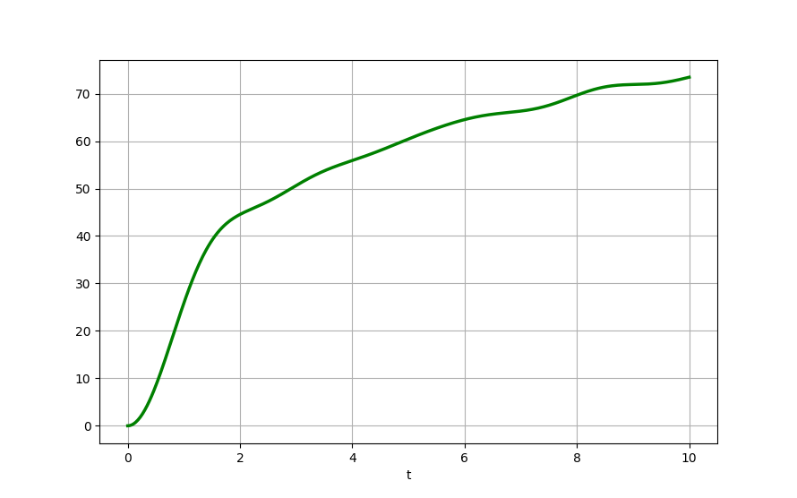
We emphasize that due to the explicit formulation of the coupled coherent state provided in (3.10), we can quantify the number of collective excitations over time. More concretely, using Proposition 2.5 the term , which is calculated in Lemma 5.1, represents the expected number of excitations generated by the interaction with the impurity. Assuming that the impurity, together with its excitations, can be interpreted as polaron-like quasi-particle, the quantity offers insight into the quasi-particle formation process. As displayed in Figure 1 on page 1 the graph shows a parabolic growth followed by a logarithmic increase as qualitative feature.
Remark 3.8.
The proof is based on the following observation: It holds by virtue of Duhamel’s formula
| (3.14) | |||
| (3.15) | |||
| (3.16) |
If the collective operators and would be exactly bosonic, i.e. the CCR holds without error, we can use the shift property Lemma 2.3 of the Weyl operator to commute to the vacuum with the cost of some inner product terms. In this case we observe with the short-hand notation and by applying Lemma 2.7 that
| (3.17) |
is exactly vanishing up to the kinetic energy term of the impurity particle since as defined in (3.10) solves the ODE and as defined in (3.11) absorbs all scalar terms.
Now by virtue of the previous statement we are able to show that the linear coupling term of the effective Hamiltonian is essential for the effective description and cannot be neglected on an approximate level.
Let
| (3.18) |
be the effective Hamiltonian without the annihilation term from the linear coupling.
Corollary 3.9.
Remark 3.10.
The result also holds for the semiclassical regime with and . The lower bound in this case is still of order .
Remark 3.11.
A priori, it is not clear why the linear coupling term cannot be neglected. Consider the almost-bosonic annihilation operator , for example, which consists of pairs of fermionic annihilation operators. Such an operator only gives a non-vanishing contribution when acting on a state which also contains at least one pair excitation. The occurrence of those pair excitations is unclear when considering the microscopic Hamiltonian (1.2). In particular, when comparing the non-bosonizable terms (2.9b) of the microscopic interaction term one might think that those terms should be generally the bosonizable terms (2.9a). However, the key observation is that the time evolved state is close to a coupled coherent state as shown in Theorem 3.4 which can be seen as superposition of product states of pair operators.
4 Proof of Theorem 3.1
In all of our estimates, we need to control the number operator acting on the time evolved state . The following statement shows that the effective time evolution preserves the order of magnitude the number of excitations:
Proposition 4.1 (Effective time evolution of the number operator).
There exists a constant such that it holds for all and
Remark 4.2.
In the semiclassical regime it holds for that and therefore the exponential bound in
is of order 1 for times .
Proof.
We want to use Grönwall’s lemma and therefore estimate the derivative
| (4.1) |
We split the difference of and consider the term with first. Insert here between and and use the commutation to obtain
| (4.2) |
We introduce the notation and to estimate
| (4.3) |
where we used Lemma A.4 and Lemma A.1 in the fourth line and the operator inequality in the fifth line. Note that for all .
The second term with can be treated by inserting and using the commutation .
| (4.4) |
We introduce the notation
| (4.5) |
Altogether it follows with the Grönwall’s lemma that
| (4.6) |
which is the desired result with since . ∎
The following statement shows that the fermionic kinetic energy term (2.8) can be approximated by the almost-bosonic kinetic energy term.
Proposition 4.3 (Approximation of the kinetic energy).
Remark 4.4.
Note that in the case of it holds and . Also note that .
Remark 4.5.
Also here the above inequality holds in the semiclassical regime with in the form of
with for times of order .
Proof.
It holds
| (4.8) |
and make use of
| (4.9) | ||||
| (4.10) |
to arrive at
| (4.11) | ||||
| (4.12) |
with the short notation .
Bounds for the error terms are readily provided in Lemma A.5 and Lemma A.6 of the appendix
| (4.13) | ||||
| (4.14) |
Furthermore use the bounds , and that all annihilate exactly two fermions to estimate
| (4.15) | ||||
| (4.16) | ||||
| (4.17) | ||||
| (4.18) |
Analogously, the term can be treated. The other terms can be estimated similarly using and Cauchy-Schwarz inequality with (A.1)
| (4.19) | ||||
| (4.20) | ||||
| (4.21) | ||||
| (4.22) | ||||
| (4.23) | ||||
| (4.24) |
Thus we derive
| (4.25) | ||||
| (4.26) |
which corresponds to the integrated version
| (4.27) |
which yields the desired result. ∎
We are now ready to give the proof of the main theorem.
Proof of of Theorem 3.1.
We employ Duhamel’s formula
| (4.28) | ||||
| (4.29) | ||||
| (4.30) |
where we used that is unitary.
From our considerations in (2.12) it follows that
Therefore by combining the bounds from Proposition 4.3 with , Lemma A.8 with and Proposition 4.1 we obtain
| (4.32) |
The prefactor is given by
| (4.33) | ||||
where we used and with and . It holds for with a sufficiently small . ∎
5 Proof of Theorem 3.4
We first collect some useful observations on the function in the following statement:
Lemma 5.1.
Let be defined as in (3.10) for , then it holds for all
where is a function independent of and monotonically increasing.
Furthermore, define by with . Then there exists a independent of such that for and sufficiently large
Remark 5.2.
Note that is for all monotonically increasing with . The same bounds hold also for in the semiclassical regime with .
Proof.
Recall that by definition it holds
| (5.1) |
with . We will first approximate and then give a upper bound.
Firstly, we approximate the -sum by an integral by identifying
| (5.2) |
with analogously to Lemma A.1. Thus, we calculate the half-sphere integral as approximation for
| (5.3) |
with total error consisting three terms: the error from (5.2), the error from approximating the discrete variables by continuous given by
| (5.4) |
and the error from the patch construction which is given by
| (5.5) |
Thus with the triangle inequality
| (5.6) |
—
We will now give an estimate for by approximating
where we used for all . Therefore
| (5.7) |
Note that using for all and for all . Thus, for
| (5.8) |
Thus by using and we obtain the desired
| (5.9) | ||||
| (5.10) |
with ∎
Lemma 5.3.
It holds for all , ,
-
(i).
,
-
(ii).
,
-
(iii).
.
Proof.
For the inequalities, we observe that for it holds
| (5.11) |
Since by assumption is bounded for each , the first statement follows. The second statement simply follows from the same calculation and recalling that . The third statement follows from Lemma A.4 and
| (5.12) |
∎
We will now give the proof of the second main theorem.
Proof of Theorem 3.4.
We use the approach as sketched in 3.8. Since the bosonic property only holds only with an error, the equality (3.17) holds only approximately:
| (5.13) |
We will first estimate the error terms and then subsequently treat the term in a separate lemma. We give an explicit expression for the first error term using Lemma 2.3 on the approximate shift property applied to in the and terms. Thus, the error of (3.17) is given by
| (5.14) |
The second error term is given by Lemma 2.7 on the time derivative of the almost-bosonic Weyl operator and therefore
| (5.15) |
Firstly, we show that the term as defined in Lemma 2.3 constitutes indeed a small error. We estimate
| (5.16) |
where we used by Lemma 5.1 and
| (5.17) | |||
| (5.18) | |||
| (5.19) |
which follows from is unitary in the first inequality, Lemma A.3 in the second inequality and Proposition 2.6 in the third inequality.
Secondly, we estimate
| (5.20) |
where we used from Lemma 2.3, the Cauchy-Schwarz inequality for the -summation, Lemma A.3 in the third inequality and in the fourth inequality we used Proposition 2.6 and (5.16).
where we used (A.2) and unitary in the third inequality and Lemma 5.1 in the last line. Using the choices of and we obtain the desired bound.
Lemma 5.4.
Proof.
We explicitly calculate the action of the Laplacian on the coupled coherent state i.e.
| (5.24) |
In total we expect, that all terms can be bounded by assumption on the initial condition on . We will first focus on the term . It holds
| (5.25) |
With
| (5.26) | ||||
| (5.27) |
it follows analogously to Lemma 2.7 that
| (5.28) |
And repeating the differentiation with
| (5.29) |
yields
| (5.30) | ||||
| (5.31) | ||||
with
| (5.32) | ||||
| (5.33) | ||||
| (5.34) | ||||
| (5.35) |
We show that each term can be bounded here by a constant at most of order .
For , we can treat all and terms with Lemma 5.1. Furthermore we use that to estimate
| (5.36) |
where we used Proposition 2.6.
For , we use a similar approach to (5.16) to obtain
| (5.37) |
For , we first observe that for
| (5.38) |
We use a similar approach to (5.20) and insert the above inequality (5.38) to obtain
| (5.39) |
For , we first calculate
| (5.40) | |||
with
| (5.41) | ||||
| (5.42) | ||||
| (5.43) | ||||
| (5.44) | ||||
| (5.45) |
We approach each term similarly to (5.16).
For , it holds
| (5.46) | |||
| (5.47) |
where we used Lemma A.4 and Lemma 5.1 in the first inequality, Lemma A.3 in the third inequality and Proposition 2.6 in the second and forth inequality. Therefore using yields
| (5.48) | |||
| (5.49) |
where we used by Lemma 5.1.
For , it holds
| (5.50) |
where we used Cauchy-Schwarz with (5.16) and Lemma 5.1 in the first inequality, Proposition 2.6 and Lemma A.3 in the second inequality. Therefore it follows
| (5.51) |
Similarly for , we estimate
| (5.54) |
using and therefore
| (5.55) |
Taking the five bounds together we finally obtain
| (5.58) |
6 Proof of Corollary 3.9
Proof of Corollary 3.9.
We observe that by the inverse triangle inequality it holds
| (6.1a) | |||
| (6.1b) | |||
The second line (6.1b) is be bounded from below by bounds of order from Theorem 3.1 and Theorem 3.4. Therefore it is sufficient to show that the first line (6.1a) is large.
The first line (6.1a) can be explicitly estimated by the same approach as in the proof of Theorem 3.4. That is use Duhamel’s formula, commute all -operators with and collect the error terms via Lemma 2.3:
| (6.2) | |||
| (6.3) | |||
| (6.4) |
with from (5.13) and where we also commuted and with such that the new error term is of the form
| (6.5) |
Note that is -dependent even though we did not include the dependence explicitly in the notation.
We employ the Cauchy-Schwarz inequality, insert our previous finding with the triangle inequality and use that is unitary to estimate
| (6.6) | |||
| (6.7) | |||
| (6.8) | |||
| (6.9) |
where we used since .
The three parts of the above inequality (6.9) can be bounded in the following:
Firstly, the error term can be bounded with (5.23) and analogously to (5.21) and (5.22):
| (6.10) |
using that for all with it holds .
Secondly, the prefactor of the integral term is bounded by Lemma A.4
| (6.11) | |||
| (6.12) |
Thirdly, we want to show that the remaining term is large:
| (6.13) |
where we used that the sum over is approximated similarly to (A.2) by integrating over the half sphere
| (6.14) |
Therefore we obtain
| (6.15) |
Note that it is well-known that for all it holds and thus for all . Also it holds for all that
since and for all . Thus we obtain
| (6.16) | ||||
| (6.17) |
which is a differentiable lower bound.
In total, we can re-write the inequality (6.9) for as the following integral inequality
| (6.20) |
Claim.
We can bound from below for all by a differentiable map which obeys the initial value problem
| (6.21) |
Proof of claim.
Assume for the proof by contradiction and set as largest open interval satisfying and for all . Note that since is differentiable such an open interval exists. It holds since and for all
and therefore
Thus we obtain the desired contradiction to being the inf of the largest set satisfying . ∎
The solution of the initial value problem (6.21) is uniquely given by
| (6.22) |
Appendix A Estimates within the bosonization framework
In this section we collect all relevant estimates of the bosonization framework which was first developed in [BNP+19, BNP+21a, BNP+21b, BPSS23] in the semiclassical regime. In addition to the references we provide brief proof sketches in order to stress the dependence of the coupling constants.
Lemma A.1 (Approximation of , [BNP+21b, Lemma 5.1]).
For and it holds
Note that by construction of .
Lemma A.2 (Approximation of ).
For and it holds
Proof.
It holds from [BNP+19, Proposition 3.1]
with . Choose for the azimuth angle of . We estimate the -sum by an appropriate surface integral over the patch
where we used and by the patch construction. Note that the integral over which excludes a collar of width can be approximated by an integral over the half-sphere
which can be calculated explicitly
Thus in total we obtain with the triangle inequality and
∎
Lemma A.3 (Estimates on the CAR error term, [BNP+21b, Lemma 5.2]).
For and the error term as defined in (2.22) satisfies , commutes with and for all it holds for all
Lemma A.4 (Pair operator bounds, [BNP+21b, Lemma 5.3]).
It holds for all and :
-
(i).
-
(ii).
-
(iii).
-
(iv).
-
(v).
-
(vi).
Lemma A.5 (Error of linearized of kinetic energy, [BNP+21b, Lemma 8.2]).
It holds for , and all
with
Proof.
Lemma A.6 (Error of bosonized kinetic energy, [BNP+21b, eq. (8.6)]).
It holds for , and all
with
Proof.
It holds and therefore
where we used in the second line bounded, Lemma A.3 in the third line, in the fourth line and Cauchy-Schwarz and Lemma A.4 in the last line.
The second statement simply follows from Cauchy-Schwarz. ∎
Lemma A.7 (Approximation of patch decomposed operators).
It holds for all
Proof.
We show that the inequality derived in [BNP+21b, eq. (4.10)] holds here independent of our adjustments. The proof in [BNP+21b, eq. (4.10)] makes use of a decomposition of the uncovered Fermi surface
into . Although the decomposition depends on the kinetic energy the final bound is independent of the kinetic energy coupling . The condition is chosen to imply due to and . Thus, one derives which gives the bound on with Cauchy-Schwarz. For the bound on insert the bound (see [BPSS23, eq. (4.10)])
into
canceling the -dependence. In total we end up with the same inequalities. ∎
Acknowledgment
We are grateful for helpful discussions with David Mitrouskas, Benjamin Schlein and Karla Schön. This work has been partially supported by SFB/Transregio TRR 352 – Project-ID 470903074.
References
- [1]
- [Ben22] Benedikter, Niels: Effective dynamics of interacting fermions from semiclassical theory to the random phase approximation. In: Journal of Mathematical Physics 63 (2022), aug, Nr. 8, S. 081101. http://dx.doi.org/10.1063/5.0091694. – DOI 10.1063/5.0091694
- [BNP+19] Benedikter, Niels ; Nam, Phan T. ; Porta, Marcello ; Schlein, Benjamin ; Seiringer, Robert: Optimal Upper Bound for the Correlation Energy of a Fermi Gas in the Mean-Field Regime. In: Communications in Mathematical Physics 374 (2019), jul, Nr. 3, S. 2097–2150. http://dx.doi.org/10.1007/s00220-019-03505-5. – DOI 10.1007/s00220–019–03505–5
- [BNP+21a] Benedikter, Niels ; Nam, Phan T. ; Porta, Marcello ; Schlein, Benjamin ; Seiringer, Robert: Bosonization of Fermionic Many-Body Dynamics. In: Annales Henri Poincaré 23 (2021), dec, Nr. 5, S. 1725–1764. http://dx.doi.org/10.1007/s00023-021-01136-y. – DOI 10.1007/s00023–021–01136–y
- [BNP+21b] Benedikter, Niels ; Nam, Phan T. ; Porta, Marcello ; Schlein, Benjamin ; Seiringer, Robert: Correlation energy of a weakly interacting Fermi gas. In: Inventiones mathematicae 225 (2021), may, Nr. 3, S. 885–979. http://dx.doi.org/10.1007/s00222-021-01041-5. – DOI 10.1007/s00222–021–01041–5
- [BPS16] Benedikter, Niels ; Porta, Marcello ; Schlein, Benjamin: Effective Evolution Equations from Quantum Dynamics. Springer International Publishing, 2016. http://dx.doi.org/10.1007/978-3-319-24898-1. http://dx.doi.org/10.1007/978-3-319-24898-1
- [BPSS23] Benedikter, Niels ; Porta, Marcello ; Schlein, Benjamin ; Seiringer, Robert: Correlation Energy of a Weakly Interacting Fermi Gas with Large Interaction Potential. In: Archive for Rational Mechanics and Analysis 247 (2023), jul, Nr. 4. http://dx.doi.org/10.1007/s00205-023-01893-6. – DOI 10.1007/s00205–023–01893–6
- [CJL+15] Cetina, Marko ; Jag, Michael ; Lous, Rianne S. ; Walraven, Jook T. ; Grimm, Rudolf ; Christensen, Rasmus S. ; Bruun, Georg M.: Decoherence of Impurities in a Fermi Sea of Ultracold Atoms. In: Physical Review Letters 115 (2015), September, Nr. 13, S. 135302. http://dx.doi.org/10.1103/physrevlett.115.135302. – DOI 10.1103/physrevlett.115.135302. – ISSN 1079–7114
- [CJL+16] Cetina, Marko ; Jag, Michael ; Lous, Rianne S. ; Fritsche, Isabella ; Walraven, Jook T. M. ; Grimm, Rudolf ; Levinsen, Jesper ; Parish, Meera M. ; Schmidt, Richard ; Knap, Michael ; Demler, Eugene: Ultrafast many-body interferometry of impurities coupled to a Fermi sea. In: Science 354 (2016), Oktober, Nr. 6308, S. 96–99. http://dx.doi.org/10.1126/science.aaf5134. – DOI 10.1126/science.aaf5134. – ISSN 1095–9203
- [FZ17] Frank, Rupert L. ; Zhou, Gang: Derivation of an effective evolution equation for a strongly coupled polaron. In: Analysis & PDE 10 (2017), feb, Nr. 2, S. 379–422. http://dx.doi.org/10.2140/apde.2017.10.379. – DOI 10.2140/apde.2017.10.379
- [JMP18] Jeblick, Maximilian ; Mitrouskas, David ; Pickl, Peter: Effective Dynamics of Two Tracer Particles Coupled to a Fermi Gas in the High-Density Limit. Version: 2018. http://dx.doi.org/10.1007/978-3-030-01602-9. In: Springer Proceedings in Mathematics & Statistics. Springer International Publishing, 2018. – DOI 10.1007/978–3–030–01602–9
- [JMPP17] Jeblick, Maximilian ; Mitrouskas, David ; Petrat, Sören ; Pickl, Peter: Free Time Evolution of a Tracer Particle Coupled to a Fermi Gas in the High-Density Limit. In: Communications in Mathematical Physics (2017). http://dx.doi.org/10.1007/s00220-017-2970-2. – DOI 10.1007/s00220–017–2970–2
- [KSN+12] Knap, Michael ; Shashi, Aditya ; Nishida, Yusuke ; Imambekov, Adilet ; Abanin, Dmitry A. ; Demler, Eugene: Time-Dependent Impurity in Ultracold Fermions: Orthogonality Catastrophe and Beyond. In: Physical Review X 2 (2012), Dezember, Nr. 4, S. 041020. http://dx.doi.org/10.1103/physrevx.2.041020. – DOI 10.1103/physrevx.2.041020. – ISSN 2160–3308
- [LP22] Lampart, Jonas ; Pickl, Peter: Dynamics of a Tracer Particle Interacting with Excitations of a Bose–Einstein Condensate. In: Annales Henri Poincaré 23 (2022), jan, Nr. 8, S. 2855–2876. http://dx.doi.org/10.1007/s00023-022-01153-5. – DOI 10.1007/s00023–022–01153–5
- [MP21] Mitrouskas, David ; Pickl, Peter: Effective pair interaction between impurity particles induced by a dense Fermi gas. In: arXiv preprint arXiv:2105.02841 (2021)
- [MS20] Myśliwy, Krzysztof ; Seiringer, Robert: Microscopic Derivation of the Fröhlich Hamiltonian for the Bose Polaron in the Mean-Field Limit. In: Annales Henri Poincaré (2020). http://dx.doi.org/10.1007/s00023-020-00969-3. – DOI 10.1007/s00023–020–00969–3
- [Saf23] Saffirio, Chiara: Weakly interacting Fermions: mean-field and semiclassical regimes. (2023), Juli. http://dx.doi.org/10.48550/ARXIV.2307.07762. – DOI 10.48550/ARXIV.2307.07762
- [SWSZ09] Schirotzek, André ; Wu, Cheng-Hsun ; Sommer, Ariel ; Zwierlein, Martin W.: Observation of Fermi Polarons in a Tunable Fermi Liquid of Ultracold Atoms. In: Physical Review Letters 102 (2009), Juni, Nr. 23, S. 230402. http://dx.doi.org/10.1103/physrevlett.102.230402. – DOI 10.1103/physrevlett.102.230402. – ISSN 1079–7114