Asymptotic Unbiased Sample Sampling to Speed Up Sharpness-Aware Minimization

Abstract

Sharpness-Aware Minimization (SAM) has emerged as a promising approach for effectively reducing the generalization error. However, SAM incurs twice the computational cost compared to base optimizer (e.g., SGD). We propose Asymptotic Unbiased Sampling with respect to iterations to accelerate SAM (AUSAM), which maintains the model’s generalization capacity while significantly enhancing computational efficiency. Concretely, we probabilistically sample a subset of data points beneficial for SAM optimization based on a theoretically guaranteed criterion, i.e., the Gradient Norm of each Sample (GNS). We further approximate the GNS by the difference in loss values before and after perturbation in SAM. As a plug-and-play, architecture-agnostic method, our approach consistently accelerates SAM across a range of tasks and networks, i.e., classification, human pose estimation and network quantization. On CIFAR10/100 and Tiny-ImageNet, AUSAM achieves results comparable to SAM while providing a speedup of over 70%. Compared to recent dynamic data pruning methods, AUSAM is better suited for SAM and excels in maintaining performance. Additionally, AUSAM accelerates optimization in human pose estimation and model quantization without sacrificing performance, demonstrating its broad practicality.

1 Introduction

The generalization capacity of a model significantly impacts its efficacy and reliability in practical applications, making it a perennially important topic in deep learning research neyshabur2017exploring ; izmailov-2018-SWA-UAI ; cha2021swad ; andriushchenko-2022-towards_understanding-ICML ; zhang2023flatness . Several studies have delved into the correlation between generalization performance and the geometry of the loss landscape keskar-2016-large_batch-ICLR ; jiang-2019-fantastic-ICLR ; wu2020adversarial ; zhang-2021-understanding-ACM . The loss landscape is complex and non-convex with many local minima of different generalization abilities hochreiter-1994-simplifying-NIPS . They observed that the flatter minima on the loss landscape tends to generalize more effectively than the sharper one. This motivates the idea of finding a flat minima during training.

Foret et al. recently introduced the Sharpness-Aware Minimization (SAM) foret-2020-SAM-ICLR algorithm, which offers a elegant approach to seek flat minima and improve generalization. The SAM prevents the model from converging to sharp minima, thereby enhancing generalization. SAM and its variants have demonstrated the state-of-the-art performance across various applications kwon-2021-asam-ICML ; jiang-2022-aesam-ICLR ; zhuang-2022-GSAM-ICLR . However, SAM lacks efficiency due to its requirement of two forward and backward in each optimization step. In recent years, various methods have been proposed to accelerate SAM. These can be roughly divided into gradient reuse methods, such as LookSAM liu-2022-looksam-CVPR , AE-SAM jiang-2022-aesam-ICLR , vSAM deng2024effective and methods for efficient SAM optimization processes, such as SAF du-2022-saf-NIPS and ESAM du-2022-ESAM-ICLR . LookSAM liu-2022-looksam-CVPR and vSAM deng2024effective periodically calculate the gradient of SAM. Although the number of gradient computations is reduced, the introduction of other operations such as gradient reuse adds extra costs. Besides, these two methods are also hard to achieve unbiased. SAF du-2022-saf-NIPS replaces SAM’s sharpness loss with trajectory loss, eliminating the need to calculate perturbations. But it requires more computation to maintain a distillation model during training. ESAM du-2022-ESAM-ICLR utilizes fewer samples to compute gradients and updates only a portion of the model. However, this approach requires more computations for sample selection, thus limiting the effect.

In this paper, we propose to dynamically sampling samples in each batch, based on the idea of asymptotically maintaining the same expected training loss between training on the sampled and original datasets. Specifically, a theoretical analysis uncovers that samples with larger gradient norms are crucial for maintaining the model’s generalization capacity. Consequently, we maintain a score of each sample with its norm during forward propagation. We exclusively select samples with higher gradient norm within each mini-batch for training. This approach significantly improves optimization efficiency while preserving the model’s generalization ability without excessive compromise. Compared to some sampling methods toneva2018empirical ; paul2021deep ; raju2021accelerating , the gradient expectation bias is reduced by asymptotic unbiased with respect to iteration.

Our contributions are summarized as follows:

• We find that utilizing mini-batch data subsets with high gradient norms for gradient computation in SAM effectively maintains the model’s generalization performance.

• We propose a asymptotic unbiased data sampling strategy to accelerate the SAM optimization process while ensuring that the generalization ability of the model does not decrease significantly.

2 Related Work

2.1 Sharpness-Aware Minimization.

The concept of searching for minima characterized as "flat minim" was introduced in hochreiter-1994-simplifying-NIPS , and extensive research has since been conducted to explore its connection with generalization andriushchenko-2022-towards_understanding-ICML ; zhang-2017-understanding-ICLR ; jiang-2019-fantastic-ICLR . Foret et al. introduced SAM foret-2020-SAM-ICLR , which aims to enhance the generalization ability of the model. SAM can be viewed as addressing a minimax optimization problem as follows:

$$\mathop{\min}\limits_{\mathbf{w}}\;{L^{SAM}}(\mathbf{w})+\lambda||\mathbf{w}||^{2}\quad\quad\text{where}\;{L^{SAM}}(\mathbf{w})=\mathop{\max}\limits_{||\bm{\varepsilon}||\leq\rho}L(\mathbf{w}+\bm{\varepsilon}),$$ (1)

where $\bm{\varepsilon}$ represents weight perturbations in an Euclidean ball with the radius $\rho$, $L^{SAM}$ is the perturbed loss, $\lambda||\mathbf{w}||^{2}$ is the standard L2 norm. In order to minimize $L^{SAM}(\mathbf{w})$, SAM utilizes Taylor expansion to search for the maximum perturbed loss in local parameter space:

$$\mathop{\arg\max}\limits_{||\bm{\varepsilon}||\leq\rho}\;L(\mathbf{w}+\bm{\varepsilon})\approx\mathop{\arg\max}\limits_{||\bm{\varepsilon}||\leq\rho}\;L(\mathbf{w})+{\bm{\varepsilon}^{T}}{\nabla_{\mathbf{w}}}L(\mathbf{w})=\mathop{\arg\max}\limits_{||\bm{\varepsilon}||\leq\rho}\;{\bm{\varepsilon}^{T}}{\nabla_{\mathbf{w}}}L(\mathbf{w}).$$ (2)

By solving Eq. (2), SAM can obtain the perturbation $\hat{\bm{\varepsilon}}=\rho{\nabla_{\mathbf{w}}}L(\mathbf{w})/||{\nabla_{\mathbf{w}}}L(\mathbf{w})||$ that maximize the loss function. By substituting the perturbation back into Eq. (1) and the gradient approximation, the gradient when SAM optimizes the weights is as follows:

$${\nabla_{\mathbf{w}}}{L^{SAM}}(\mathbf{w})\approx{\nabla_{\mathbf{w}}}L(\mathbf{w}+\bm{\hat{\varepsilon}})\approx{\nabla_{\mathbf{w}}}L(\mathbf{w}){|_{\mathbf{w}+\bm{\hat{\varepsilon}}}}.$$ (3)

From Eq. (2) and Eq. (3), we observe that SAM necessitates two forward and backward operations to update weights once. This makes the computational overhead of SAM twice that of the basic optimizer.

2.2 Methods of Accelerating SAM.

In this section, we discuss related work on gradient reuse methods, methods for efficient SAM optimization processes, and dynamic data pruning methods.

Gradient Reuse Methods. The motivation of reusing gradients is to reduce the number of SAM updates during training. LookSAM liu-2022-looksam-CVPR employs SAM at every $k$ iterations and reuse previous gradients in other iterations. This periodic strategy makes most optimization steps without SAM. However, reusing gradients and other steps introduce additional time overhead. AE-SAM jiang-2022-aesam-ICLR adaptively employs SAM based on the loss landscape geometry. However, it requires sharpness to be evaluated at each optimization step.

Methods for efficient SAM optimization processes. These methods are to improve the efficiency of each step of SAM. SAF and MESA du-2022-saf-NIPS employ trajectory loss to approximate sharpness. However, SAF and MESA do not employ direct weight perturbations to facilitate SAM in escaping local minimum regions. Furthermore, SAF necessitates significant memory resources to store output results for all data, whereas MESA requires the maintenance of an Exponential Moving Average (EMA) model throughout training. ESAM du-2022-ESAM-ICLR uses fewer samples to compute the gradients and only updates part of the model in the SAM’s second step. However, ESAM requires a lot of extra computation when selecting samples and gradients should be computed for almost every weight during backward propagation. This paper proposes a sample sampling strategy that does not require substantial additional computational resources, aiming to accelerate both the forward and backward sampling of the SAM algorithm, thus improving SAM’s optimization efficiency.

Dynamic Data Pruning Methods. Dynamic data pruning aims to save the training cost by reducing the number of iterations for training. toneva2018empirical ; paul2021deep The pruning process is conducted during training and sample information can be obtained from current training. Dynamically prunes the samples based on easily attainable scores, e.g., loss values, during the training without trials. raju2021accelerating proposes three different data selection criteria in dynamic data pruning. Uncertainty sampling preferentially selects the sample with the lowest confidence in the current prediction of the model. $\varepsilon$-greedy approach is inspired by reinforcement learning. The upper-confidence bound (UCB) approach suggests prune samples based on the upper confidence bound of their losses. InfoBatch qin-2024-infobatch randomly prunes less informative samples based on loss distribution and rescales remaining samples’ gradients to approximate the original gradient. However, these methods are not specific to SAM.

3 Method

3.1 Principle of Sampling

Principally, we aim to select a subset of samples from each mini-batch during training, thereby reducing the computational costs of SAM’s forward and backward propagation. One question is whether the perturbation loss computed from a subset closely approximates that computed from the full mini-batch.

Theorem 1.

Suppose we select $N$ samples from a mini-batch $\mathbf{B}$ of size $K$, denoting them as $\hat{\mathbf{B}}$ ($\hat{{x}_{i}}\in\hat{\mathbf{B}}$, $i=1,2,...,N$), and represent the remaining set of $M(M=K-N)$ samples as $\check{\mathbf{B}}$ ($\check{{x}_{i}}\in\check{\mathbf{B}}$, $i=1,2,...,M$). Let $\bm{\varepsilon}_{\mathbf{B}}$ and $\bm{\varepsilon}_{\hat{\mathbf{B}}}$ represent the parameter perturbations in SAM obtained through the set $\mathbf{B}$ and $\hat{\mathbf{B}}$, respectively. The difference between the Perturbation Loss computed by the Full mini-batch (PLF) and the Perturbation Loss computed by the Sampled (PLS) samples is bounded as follows:

$$\bigg{|}\underbrace{\max_{\|{\bm{\varepsilon}_{\mathbf{B}}}\|\leq\rho}\big{[}L_{\mathbf{B}}(\mathbf{w}+{\bm{\varepsilon}_{\mathbf{B}}})-L_{\mathbf{B}}(\mathbf{w})\big{]}}_{\text{PLF}}-\underbrace{\max_{\|{\bm{\varepsilon}_{\hat{\mathbf{B}}}}\|\leq\rho}\big{[}L_{\hat{\mathbf{B}}}(\mathbf{w}+{\bm{\varepsilon}_{\hat{\mathbf{B}}}})-L_{\hat{\mathbf{B}}}(\mathbf{w})\big{]}}_{\text{PLS}}\bigg{|}\leq\frac{\rho}{M}\sum_{i=1}^{M}{\left\|{\nabla_{\mathbf{w}}}{L_{\check{\mathbf{x}}_{i}}}(\mathbf{w})\right\|}.$$ (4)

Theorem 1 demonstrates that the upper bound on the perturbation loss difference between the full mini-batch and the sampled samples is smaller when the gradient norm of the un-sampled samples is smaller. One sampling method is to use the gradient norm of each sample as a criterion to determine whether the sample is selected. However, Theorem 1 face the problem: how to efficiently compute the gradient norm of each sample $\left\|{{\nabla_{\mathbf{w}}}{L_{\mathbf{x}_{i}}}(\mathbf{w})}\right\|$ as the criterion before sampling?

Directly computing the gradient norm for each sample in every iteration is impractical. This is because it requires iterating through each sample individually to obtain its gradient and compute the gradient norm, demanding significant computational resources.

3.2 Efficiently Approximating Gradient Norms

Lemma 1.

Given the parameter perturbation ${\bm{\varepsilon}_{\mathbf{B}}}$ and the gradient ${{\nabla_{\mathbf{w}}}{L_{\mathbf{B}}}(\mathbf{w})}$ for the mini-batch data $\mathbf{B}$. The original loss and perturbation loss of sample $\mathbf{x}_{i}\in\mathbf{B}$ , denote as ${L_{\mathbf{x}_{i}}}(\mathbf{w})$ and ${L_{\mathbf{x}_{i}}}(\mathbf{w}+{\bm{\varepsilon}_{\mathbf{B}}})$ respectively. The gradient norm of sample $\mathbf{x}_{i}$, denote as $\left\|{{\nabla_{\mathbf{w}}}{L_{\mathbf{x}_{i}}}(\mathbf{w})}\right\|$, is approximated as follows:

$$\left\|{{\nabla_{\mathbf{w}}}{L_{\mathbf{x}_{i}}}(\mathbf{w})}\right\| \approx\frac{C}{\rho}\cdot\bigg{|}\underbrace{{{L_{\mathbf{x}_{i}}}(\mathbf{w}+{\bm{\varepsilon}_{\mathbf{B}}})-{L_{\mathbf{x}_{i}}}(\mathbf{w})}}_{DLP}\bigg{|},$$ (5)

where $C={\left\|{{\nabla_{\mathbf{w}}}{L_{\mathbf{B}}}(\mathbf{w})}\right\|}\left\|{\frac{1}{{{\nabla_{\mathbf{w}}}{L_{\mathbf{B}}}(\mathbf{w})}}}\right\|$ is the same constant for each sample in the mini-batch $\mathbf{B}$.

Lemma 1 discovers that the gradient norm of sample $\mathbf{x}_{i}$ can be approximated by the Difference in Loss before and after Perturbation (hereinafter referred to as DLP), i.e., ${{L_{\mathbf{x}_{i}}}(\mathbf{w}+{\bm{\varepsilon}_{\mathbf{B}}})-{L_{\mathbf{x}_{i}}}(\mathbf{w})}$. In addition, the absolute value of the DLP is proportional to the gradient norm $\left\|{{\nabla_{\mathbf{w}}}{L_{\mathbf{x}_{i}}}(\mathbf{w})}\right\|$, i.e.,

$$d_{{\mathbf{x}_{i}}}=\left|{{L_{\mathbf{x}_{i}}}(\mathbf{w}+{\bm{\varepsilon}_{\mathbf{B}}})-{L_{\mathbf{x}_{i}}}(\mathbf{w})}\right|\propto\left\|{{\nabla_{\mathbf{w}}}{L_{\mathbf{x}_{i}}}(\mathbf{w})}\right\|.$$ (6)

Therefore, rather than estimating $\left\|{{\nabla_{\mathbf{w}}}{L_{\mathbf{x}_{i}}}(\mathbf{w}_{t})}\right\|$, we compute $d_{{\mathbf{x}_{i}}}$ as the sampling criterion. For the $T$-th epoch, we estimate $d^{T}_{{\mathbf{x}_{i}}}$ from the historical absolute values of the DLP (${d^{t}_{{\mathbf{x}_{i}}}},t\in\{0,\ldots,T-1\}$) for sample $\mathbf{x}_{i}$ before training. We have propose two promising method as follows:

Recent used approach. One approach estimates the gradient norm of sample ${{\mathbf{x}_{i}}}$ at epoch $T$ by $d_{{\mathbf{x}_{i}}}^{T-1}$ at the previous epoch, as follows:

$$g_{{\mathbf{x}_{i}}}^{T}=d_{{\mathbf{x}_{i}}}^{T-1}={\left|{L_{{\mathbf{x}_{i}}}(\mathbf{w}_{T-1}+{\bm{\varepsilon}_{\mathbf{B}}})-L_{{\mathbf{x}_{i}}}(\mathbf{w}_{T-1})}\right|},$$ (7)

where $g_{{\mathbf{x}_{i}}}^{T}$ is the estimated value, which will be used as an indicator for our sampling criterion. We compute $d_{{\mathbf{x}_{i}}}^{t}$ for each sample $\mathbf{x}_{i}$ during training in each epoch $t$ and store it to decide whether the sample should be selected in the current epoch. The time and storage complexity of this approach are both $O(n)$, where $n$ is the number of samples in the dataset. We denote this approach as AUSAM-l.

Averaged approach. To enhance the accuracy of evaluating the gradient norm for each sample, we estimate the current gradient norm by averaging the historical DLP values for each sample. The average DLP of samples $\mathbf{x}_{i}$ in a mini-batch $\mathbf{B}$ at epoch $T$ is given as follows:

$$g_{{\mathbf{x}_{i}}}^{T}=\frac{1}{{T-1}}\sum\limits_{t=1}^{T-1}{d}_{{\mathbf{x}_{i}}}^{t}={\frac{1}{{T-1}}}\sum\limits_{t=1}^{T-1}{\left|{L_{{\mathbf{x}_{i}}}(\mathbf{w}_{t}+{\bm{\varepsilon}_{\mathbf{B}}})-L_{{\mathbf{x}_{i}}}(\mathbf{w}_{t})}\right|},$$ (8)

where ${L_{{\mathbf{x}_{i}}}}(\mathbf{w}_{t})$ and ${L_{{\mathbf{x}_{i}}}}(\mathbf{w}_{t}+{\bm{\varepsilon}_{\mathbf{B}}})$ are the original loss and the perturbation loss of data $\mathbf{x}_{i}$ at epoch $t$. The time and storage complexity of this approach are also both $O(n)$. We ultimately choose to compute our sampling criterion using this method, with Theorem 2 providing the related theoretical foundation, and the experiments detailed in Appendix B.1.

3.3 Sampling Strategy

To ensure that samples with small $g_{{\mathbf{x}_{i}}}^{T}$ are not overlooked, we sample each sample with a probability. The probability of each sample at epoch $T$ is given as follows:

$${p^{T}_{\mathbf{x}_{i}}}=\frac{{{{g}^{T}_{{\mathbf{x}_{i}}}}}}{{\sum\nolimits_{i=1}^{K}{{{g}^{T}_{{\mathbf{x}_{i}}}}}}},$$ (9)

where $p^{T}_{\mathbf{x}_{i}}$ denotes the sampling probability of sample $\mathbf{x}_{i}$ in mini-batch $\mathbf{B}$ at epoch $T$, $\mathbf{x}_{i}\in\mathbf{B}$ with the size of $K$. To control the ratio of the maximum and minimum sampling probabilities, we normalize ${g}^{T}_{{\mathbf{x}_{i}}}$ using min-max normalization as follows:

$$\tilde{g}_{{\mathbf{x}_{i}}}={s_{min}}+\frac{{{g}^{T}_{{\mathbf{x}_{i}}}-{g}_{\mathbf{B}}^{min}}}{{{g}_{\mathbf{B}}^{max}-{g}_{\mathbf{B}}^{min}}}({s_{max}}-{s_{min}}),$$ (10)

where $s_{min}$ and $s_{max}$ are the lower and upper bounds of the normalization, respectively. ${g}_{\mathbf{B}}^{max}$ and ${g}_{\mathbf{B}}^{min}$ denote the maximum and minimum values of ${g}_{{\mathbf{x}_{i}}}$ within the mini-batch $\mathbf{B}$, respectively. We substitute ${g}_{{\mathbf{x}_{i}}}$ with $\tilde{g}_{{\mathbf{x}_{i}}}$ in Eq. (9) to calculate the probability ${p^{T}_{\mathbf{x}_{i}}}$. In addition, we designate a hyperparameter, $\alpha$, to denote the proportion of samples selected from a mini-batch $\mathbf{B}$ of size $K$, meaning $\alpha K$ samples are sampled from it. The time and storage complexity of this process are $O(n)$ and $O(1)$, respectively.

Initialization of AUSAM: We gradually select samples with large gradient norm for the stable initialization of training. We define a fixed epoch $E_{start}$ and allow $s_{max}$ to be a floating value before epoch $E_{start}$, gradually increasing from $s_{min}$ to the specified value of $s_{max}$. This enables samples with larger average gradient norms to be increasingly prioritized for selection during training. Algorithm 1 shows the overall proposed algorithm.

Speed up ratio of SAM: Suppose that the time complexity of optimizing the model with SAM is $O(T)$. We can roughly divide the $T$ into the two forward and backward time $T_{f}$ and the remaining time $T_{b}$. Our method can theoretically reduce the two forward and backward time to $\alpha T_{f}$. When $T_{b}$ is sufficiently small, our method achieves nearly $O(0.5T)$ when $\alpha=0.5$, which is almost as fast as the base optimizer.

3.4 Theoretical Analysis

Assumption 1.

(Smoothness). $L(\mathbf{w})$ is $\tau$-Lipschitz smooth in $\mathbf{w}$, i.e., $\left\|{\nabla L(\mathbf{w})-\nabla L(\mathbf{v})}\right\|\leq\tau\left\|{\mathbf{w}-\mathbf{v}}\right\|$.

Assumption 2.

(Bounded gradients). By the assumption that an upper bound is exists on the gradient of sampled set $\hat{\mathbf{B}}$ from each mini-batch. There exists $G>0$ for $\hat{\mathbf{B}}$ such that $\mathbb{E}\left[{\left\|{\nabla L_{\hat{\mathbf{B}}}(\mathbf{w})}\right\|}\right]\leq G$.

Assumption 3.

(Bounded variance of stochastic gradients). Given the training set $\mathbf{D}$ and a sampled set $\hat{\mathbf{B}}\in\mathbf{D}$. There exists $\sigma\geq 0$, the variance of the sampled set of size $\alpha K$ is bounded by $\mathbb{E}\left[{{{\left\|{\nabla{L_{\hat{\mathbf{B}}}}(\mathbf{w})-\nabla{L_{\mathbf{D}}}(\mathbf{w})}\right\|}^{2}}}\right]\leq\frac{\sigma^{2}}{\alpha K}$.

Theorem 2.

Suppose Assumption 1 and 2 hold. Let learning rate ${\eta_{t}}=\frac{{{\eta_{0}}}}{{\sqrt{t}}}$, ${\eta_{0}}$ represents the initial learning rate, and there are $I$ iterations in one epoch. The deviation between the average gradient norm of sample $\mathbf{x}_{i}$ over $T-1$ epochs and the gradient norm at the $T$-th epoch is bounded within a specific range, defined as follows:

$$\left|{\left\|{\nabla{L_{{\mathbf{x}_{i}}}}({\mathbf{w}_{T}})}\right\|-\frac{1}{{T-1}}\sum\limits_{t=1}^{T-1}{\left\|{{\nabla_{\mathbf{w}}}{L_{{\mathbf{x}_{i}}}}({\mathbf{w}_{t}})}\right\|}}\right|\leq\frac{{\tau IG{\eta_{0}}(2\sqrt{T-1}-1)}}{{T-1}}.$$ (11)

From Theorem 2, it’s evident that the error gradually decreases as $T$ increases. This suggests the viability of substituting the current gradient norm with the average gradient norm (Eq. 8).

Algorithm 1 Pseudocode of the proposed Method

Require: The training dataset, the learning rate $\eta$, the batch size $K$, parameters $\alpha$, $\rho$, $s_{min}$ and $s_{max}$.

1:  for $t=1,2,\cdot\cdot\cdot$ do

2:     Sample a mini-batch data $\mathbf{B}$;

3:     Calculate the probability of each sample in $\mathbf{B}$ being selected by Eq. (9);

4:     Sampling $\alpha K$ samples from $\mathbf{B}$ to form a sampling set $\hat{\mathbf{B}}$, $(\mathbf{x}_{i}\in\hat{\mathbf{B}},i=1,2,...,\alpha K)$;

5:     Compute the loss of each selected sample $L_{\mathbf{x}_{i}}(\mathbf{w}_{t})$ and gradient of all selected samples $\nabla_{\mathbf{w}}{L_{\hat{\mathbf{B}}}}(\mathbf{w}_{t})$.

6:     Compute perturbation $\hat{\bm{\varepsilon}}=\rho\frac{\nabla_{\mathbf{w}}L_{\hat{\mathbf{B}}}(\mathbf{w}_{t})}{||{\nabla_{\mathbf{w}}}L_{\hat{\mathbf{B}}}(\mathbf{w}_{t})||}$, perturbation loss $L_{\hat{\mathbf{B}}}(\mathbf{w}_{t}+\bm{\varepsilon})$ and gradient after perturbation $\nabla_{\mathbf{w}}{L_{\hat{\mathbf{B}}}}(\mathbf{w}_{t}+\bm{\varepsilon})$.

7:     Update the weights by ${\mathbf{w}_{t+1}}={\mathbf{w}_{t}}-\eta\nabla_{w}{L_{\hat{\mathbf{B}}}}(\mathbf{w}_{t}+\bm{\varepsilon})$;

8:     Update the indicator for our sampling criterion for each selected sample according to Eq. (8).

9:  end for

Theorem 3.

Suppose Assumptions 1 and 3 hold. Let $K$ be the mini-batch size, $\alpha$ is the sampling rate. For all learn rate $\eta\leq\frac{1}{\tau}$ and $\rho\leq\frac{1}{{4\tau}}$, the algorithm satisfies:

$$\mathbb{E}\left[\sum\limits_{t=1}^{T}{{{\left\|\nabla L_{\mathbf{D}}({\mathbf{w}_{t}})\right\|}^{2}}}\right]\leq\frac{{16}}{{7\eta T}}\left({L[({\mathbf{w}_{0}})]-E[L({\mathbf{w}_{T}})]}\right)+\frac{{17\eta\tau{\sigma^{2}}}}{{7\alpha K}}.$$ (12)

We observe that the convergence of sample selection for training remains feasible, with selecting more samples from each mini-batch resulting in tighter bounds.

Theorem 4.

Assuming all samples $\mathbf{x}$ from $\mathbf{D}$ are drawn from continuous distribution $q(\mathbf{x})$. $p^{t}_{\mathbf{x}}$ is the probability that sample $\mathbf{x}$ is sampled in the $t$-th epoch. The perturbation of SAM is assumed to be the theoretical perturbation over the entire dataset $\mathbf{D}$, i.e. ${\bm{\varepsilon}_{\mathbf{D}}}=\rho{{{\nabla_{\mathbf{w}}}{L_{D}}({\mathbf{w}_{t}})}}//{{\left\|{{\nabla_{\mathbf{w}}}{L_{D}}({\mathbf{w}_{t}})}\right\|}}$. The difference between the expected loss of full dataset and the expected loss of sampled subsets $\hat{\mathbf{D}}$ can be expressed as follows:

$$\left|{\mathop{\mathbb{E}}\limits_{\mathbf{x}\in\mathbf{D}}\left[{\mathop{\max}\limits_{\left\|{{\bm{\varepsilon}_{\mathbf{x}}}}\right\|\leq\rho}[{L_{\mathbf{x}}}({\mathbf{w}_{t}}+{\bm{\varepsilon}_{\mathbf{D}}})-{L_{\mathbf{x}}}({\mathbf{w}_{t}})]}\right]-\mathop{\mathbb{E}}\limits_{{\mathbf{x}}\in\hat{\mathbf{D}}}\left[{\mathop{\max}\limits_{\left\|{{\bm{\varepsilon}_{\mathbf{x}}}}\right\|\leq\rho}[{L_{\mathbf{x}}}({\mathbf{w}_{t}}+{\bm{\varepsilon}_{\mathbf{D}}})-{L_{\mathbf{x}}}({\mathbf{w}_{t}})]}\right]}\right|$$ (13)

$$\leq\rho\int_{\mathbf{x}}{(1-p_{\mathbf{x}}^{t})\left\|{{\nabla_{\mathbf{w}}}{L_{\mathbf{x}}}({\mathbf{w}_{t}})}\right\|q({\mathbf{x}})}d{\mathbf{x}}.$$

During the stage where SAM finds the internal maximum, Theorem 4 indicates that if we choose samples with larger gradient norms $\left\|{{\nabla_{\mathbf{w}}}{L_{\mathbf{x}}}(\mathbf{w}_{t})}\right\|$ with greater probability $p^{t}_{\mathbf{x}}$, the expected error generated by these samples will be smaller compared to randomly selected samples. As $t$ increases, the gradient norm of sample $\mathbf{x}$ will theoretically gradually decrease, and the expected error will also gradually decrease. We still need to use these sampled samples in the gradient descent phase of SAM. They help find the maximum loss in the parametric neighborhood space. Sampling other samples means not optimizing for this maximum loss, which goes against the SAM principle. Also, as $t$ increases, samples with smaller gradient norms become less influential. Therefore, we choose samples with larger gradient norms to better represent the full mini-batch. All proofs are in Appendix A.

4 Experimental Results

4.1 Setup

Datasets and Models. We conduct experiments on CIFAR-10, CIFAR-100 krizhevsky2009learning and Tiny-ImageNet le-2015-tiny image classification benchmark datasets. We employ a variety of architectures, i.e. ResNet-18 he2016deep , WideResNet-28-10 zagoruyko2016wide and PyramidNet-110 han2017deep on CIFAR-10 and CIFAR-100, ResNet-18, ResNet-50 he2016deep , and MobileNetv1 howard2017mobilenets on Tiny-ImageNet chrabaszcz2017downsampled , to evaluate the performance and training efficiency.

Baselines. We take the vanilla SGD and SAM foret-2020-SAM-ICLR as baselines. To comprehensively evaluate the performance, we have also chosen some efficient methods ESAM du-2022-ESAM-ICLR , LookSAM liu-2022-looksam-CVPR , SAF du-2022-saf-NIPS , MESA du-2022-saf-NIPS and AE-SAM jiang-2022-aesam-ICLR for comparison. These methods are the follow-up works of SAM that aim to enhance efficiency. Additionally, we choose InforBatch qin-2024-infobatch , an advanced dynamic data pruning method, and apply it to SAM. We also establish a dynamic pruning baseline, referred to as "SAM+Random," which randomly selects half of the samples in each batch.

Implementation Details. We train all the models 200 epochs using a batch size of 128 with cutout regularization devries2017improved and cosine learning rate decay loshchilov2016sgdr for all methods on CIFAR-10 and CIFAR-100. For the proposed method, we set $s_{min}=0.1$ in our experiments, $s_{max}=0.5$ for ResNet-18 and WideResNet-28-10, $s_{max}=1$ for PyramidNet-110. Typically, $s_{max}$ is set to $1$, though for smaller networks, it may be reduced further. This adjustment is motivated by the heightened impact of omitting samples with small gradient norms on smaller networks. Lowering $s_{max}$ increases the chances for samples with smaller gradient norms to be chosen.

For Tiny-ImageNet, we also train ResNet-18, ResNet-50 and MobileNetv1 howard2017mobilenets 200 epochs using a batch size of 128 with cutout and cosine learning rate decay. For ResNet-18, ResNet-50, we use the $64\times 64$ resolution images and transform the first convolution of the models to a $3\times 3$ convolution. For MobileNetv1, we resize the original image to $224\times 224$.

We rename AUSAM as AUSAM-$\alpha$ according to the value of $\alpha$ when reporting the results. Each experiment was repeated three times using different random seeds to calculate the standard deviation, and the results are reported on average. We implement AUSAM in Pytorch and train models on a single NVIDIA GeForce RTX 3090.

4.2 Parameter Studies

Parameter study of $\bm{\alpha}$.

We study the effect of $\alpha$ on accuracy and optimization efficiency using Resnet-18 and WideResNet-28-10 on the CIFAR-100 dataset. $\alpha$ determines the number of samples in each mini-batch, significantly influencing both the efficiency and accuracy of model training. The corresponding results are summarized in Tab. 1. ResNet-18, with its smaller network structure, necessitates less time for both forward and backward computations. As a result, AUSAM exhibits a smaller speedup ratio compared to SAM. Conversely, WideResNet demands more time for these computations, resulting in a larger speedup ratio for AUSAM over SAM. Additionally, as $\alpha$ increases, the speedup ratio of AUSAM gradually decreases. This is because forward and backward propagation become more time-consuming with more samples selected per mini-batch. Generally, we set $\alpha=0.5$, meaning that half of the samples are selected from each mini-batch. In theory, when $\alpha=0.5$, the speed of AUSAM can nearly match that of the base optimizer, such as SGD. However, in these two networks, the time spent on other operations, such as data loading, is non-negligible compared to the time spent on forward and backward. Therefore, it cannot achieve the same speed as SGD.

Table 1: Parameter Study of $\alpha$.

$\alpha$	Resnet-18		Wideresnet-28-10
	Accuracy	Image/s	Accuracy	Image/s
SAM	81.04$\pm$0.29	1866(100%)	84.71$\pm$0.21	351(100%)
0.4	80.18$\pm$0.26	2424(130%)	84.44$\pm$0.31	780(202%)
0.5	80.67$\pm$0.05	2467(132%)	84.62$\pm$0.26	627(179%)
0.6	80.69$\pm$0.15	2217(119%)	84.73$\pm$0.29	533(152%)
0.7	80.92$\pm$0.17	2117(114%)	84.66$\pm$0.07	471(134%)

Table 2: The results of the proposed method and the comparison methods on CIFAR-10 and CIFAR-100 dataset. The numbers in parentheses (·) indicate the ratio of corresponding method’s training speed to SAM’s. $\uparrow$ means that the larger the reported results are better. The best accuracy is in bold and the second best is underlined.

	CIFAR-10		CIFAR-100
ResNet-18	Accuracy $\uparrow$	Images/s $\uparrow$	Accuracy $\uparrow$	Images/s $\uparrow$
SGD	96.23$\pm$0.11	3153(170%)	79.84$\pm$0.45	3181(171%)
SAM	96.79$\pm$0.03	1855(100%)	81.04$\pm$0.29	1866(100%)
LookSAM-5	96.47$\pm$0.13	2134(115%)	80.48$\pm$0.24	2115(113%)
ESAM	96.58$\pm$0.13	1936(104%)	80.47$\pm$0.31	1953(105%)
ESAM1	96.56$\pm$0.08	2409(140%)	80.41$\pm$0.10	2423(140%)
SAF	96.15$\pm$0.11	2733(147%)	80.03$\pm$0.43	2736(147%)
SAF2	96.37$\pm$0.02	3213(194%)	80.06$\pm$0.05	3248(192%)
MESA2	96.24$\pm$0.02	2780(168%)	79.79$\pm$0.09	2793(165%)
AUSAM-0.5	96.52$\pm$0.01	2450(132%)	80.67$\pm$0.05	2467(132%)
AUSAM-0.6	96.59$\pm$0.14	2274(123%)	80.69$\pm$0.15	2217(119%)
WideResNet-28-10	Accuracy $\uparrow$	Images/s $\uparrow$	Accuracy $\uparrow$	Images/s $\uparrow$
SGD	96.91$\pm$0.06	680(195%)	82.47$\pm$0.30	685(195%)
SAM	97.44$\pm$0.04	349(100%)	84.71$\pm$0.21	351(100%)
LookSAM-5	97.13$\pm$0.04	537(154%)	83.52$\pm$0.09	552(157%)
ESAM	97.41$\pm$0.07	502(144%)	84.71$\pm$0.32	494(141%)
ESAM1	97.29$\pm$0.11	550(139%)	84.51$\pm$0.01	545(139%)
SAF	96.96$\pm$0.09	639(183%)	82.57$\pm$0.18	639(182%)
SAF2	97.08$\pm$0.15	727(198%)	83.81$\pm$0.04	729(197%)
MESA2	97.16$\pm$0.23	617(168%)	83.59$\pm$0.24	625(169%)
AUSAM-0.5	97.3$\pm$0.06	624(179%)	84.62$\pm$0.26	627(179%)
AUSAM-0.6	97.49$\pm$0.05	530(152%)	84.73$\pm$0.29	533(152%)
PyramidNet-110	Accuracy $\uparrow$	Images/s $\uparrow$	Accuracy $\uparrow$	Images/s $\uparrow$
SGD	97.14$\pm$0.08	548(195%)	83.38$\pm$0.21	544(196%)
SAM	97.69$\pm$0.09	281(100%)	86.06$\pm$0.16	278(100%)
LookSAM-5	97.22$\pm$0.05	339(121%)	83.76$\pm$0.45	350(126%)
ESAM	97.59$\pm$0.17	322(115%)	85.32$\pm$0.03	321(116%)
ESAM1	97.81$\pm$0.01	401(139%)	85.56$\pm$0.05	381(138%)
SAF	96.96$\pm$0.05	501(178%)	83.66$\pm$0.34	502(181%)
SAF2	97.34$\pm$0.06	391(202%)	84.71$\pm$0.01	397(200%)
MESA2	97.46$\pm$0.09	332(171%)	84.73$\pm$0.14	339(171%)
AUSAM-0.5	97.63$\pm$0.04	493(175%)	85.68$\pm$0.03	490(176%)
AUSAM-0.6	97.72$\pm$0.09	425(151%)	85.78$\pm$0.06	424(153%)
$1$ We report the results in du-2022-ESAM-ICLR . But failed to reproduce them using the officially released codes.
$2$ We report the results in du-2022-saf-NIPS . We reproduced it ourselves following the algorithmic flow of SAF.

4.3 Comparison to SOTAs

The experimental results on CIFAR-10 and CIFAR-100 are presented in Tab. 2. We observe that AUSAM achieves significantly higher accuracy compared to SGD. Furthermore, in comparison to LookSAM, ESAM, and AE-SAM, our results outperform theirs in most cases. This demonstrates that AUSAM can successfully preserve the model’s generalization ability during the training process. Probably because AUSAM essentially reduces the batch size, which helps to improve the generalization of the model he－2019－control . Although the number of iterations for the whole training did not grow, the selected samples accelerated the training of the model. We also achieve superior results compared to SAF and MESA. Because SAF and MESA optimize the sharpness from multiple previous iteration to the current iteration, which is different from the sharpness of the current iteration.

These experiments demonstrate that AUSAM exhibits about 70% faster training than SAM while achieving comparable accuracy. In the case of ResNet-18, the benefits of AUSAM are not fully apparent due to the inherently shorter duration required for both forward and backward propagation during the optimization process. When the model is larger, such as WideResNet-28-10 and PyramidNet-110, AUSAM is more advantageous and faster. LookSAM reduces the number of SAM computations but requires additional operations such as computing gradient projections. ESAM needs to calculate the loss of all samples first and then select the samples. SAF sacrifices memory to optimize efficiency and achieves almost the same speedup as SGD.

Table 3: The results of SGD, SAM and AUSAM on Tiny-ImageNet. The best accuracy is in bold.

	ResNet-18		ResNet-50		MobileNetv1
Methods	Accuracy	Images/s	Accuracy	Images/s	Accuracy	Images/s
SGD	61.88$\pm$0.31	728(198%)	65.60$\pm$0.51	191(201%)	58.12$\pm$0.4	547(189%)
SAM	64.43$\pm$0.08	368(100%)	67.69$\pm$0.10	95(100%)	58.49$\pm$0.38	289(100%)
AUSAM-0.5	64.37$\pm$0.03	704(191%)	66.60$\pm$0.21	185(195%)	58.55$\pm$0.23	534(185%)
AUSAM-0.6	64.49$\pm$0.39	551(151%)	66.65$\pm$0.34	158(166%)	58.94$\pm$0.24	464(161%)

The experimental results on Tiny-ImageNet are presented in Tab. 3. Due to the larger image resolution of Tiny-ImageNet compared to CIFAR-10 and CIFAR-100, the network necessitates more time for both forward and backward computations, leading to a higher acceleration ratio for AUSAM. With $\alpha=0.5$, AUSAM achieves over 85% acceleration across all three models. On ResNet-18 and MobileNetv1, AUSAM achieves results comparable to SAM. AUSAM approaches SGD speed while maintaining higher accuracy than SGD on ResNet-50.

4.4 Comparison to Dynamic Data Pruning

Data pruning is directed towards achieving lossless performances while minimizing overall expenses. It prunes part of the less informative samples at each epoch and trains with the remaining samples. We apply the advanced dynamic data pruning method InfoBatch qin-2024-infobatch on the CIFAR-100 and conduct experiments using SGD and SAM. SAM+Info* represents the use of InfoBatch during the first loss calculation of SAM, while SAM+Info indicates its use during the second loss calculation of SAM. The results are presented in Tab. 4. We observe that while InfoBatch enhances optimization efficiency, it does not ensure lossless accuracy for SAM on CIFAR-100. Most dynamic data pruning methods struggle to effectively leverage the two losses before and after perturbation in SAM. These methods typically directly select samples with larger original losses, but these samples may not necessarily exhibit larger losses in the parameter neighborhood space, which is not in line with SAM’s optimization principle.

Table 4: The Results of using InfoBatch to accelerate SAM.

Methods	Accuracy $\uparrow$	Images/s $\uparrow$
SGD	79.79$\pm$0.14	3156(177%)
SAM	81.24$\pm$0.10	1782(100%)
SGD+Info	79.21$\pm$0.24	3502(197%)
SAM+Info*	79.68$\pm$0.26	2438(137%)
SAM+Info	79.57$\pm$0.09	2487(140%)
SAM+Random	80.56$\pm$0.19	2144(120%)

4.5 Application to Human Pose Estimation

2D Human Pose Estimation (HPE) aims to localize body joints from a single image. We apply SAM and AUSAM to human pose estimation to validate the generality of the methods. The chosen approach is SimCC li2022simcc . The key idea of SimCC is to treat human pose estimation as two classification tasks, one for vertical and one for horizontal coordinates. It aims to minimize quantization error by dividing each pixel into multiple bins. We use SAM and AUSAM as optimization methods for the SimCC, and conducted experiments on the MP$\mathrm{II}$ dataset andriluka14cvpr . The results are reported in Appendix B.3. The results show that both SAM and AUSAM can be applied to SimCC. AUSAM accelerates the training speed while maintaining the results of SAM.

4.6 Application to Quantization-Aware Training

Neural network quantization reduces computational demands by lowering weight and activation precision, enabling efficient deployment on edge devices without compromising model performance jacob-2018-quantization ; esser2020learned ; wei2021qdrop ; nagel2022overcoming . We employ AUSAM as the optimization method for QAT jacob-2018-quantization to demonstrate its broader applicability. We utilized SGD, SAM, and AUSAM to quantize the parameters of ResNet-18 and MobileNetv1 to W2A4 on the CIFAR-10 dataset, and the results are presented in Appendix B.4. Although the time required for both forward and backward is significantly reduced after model quantization, experimental results show that AUSAM can still accelerate the optimization speed while maintaining performance.

5 Conclusions

The findings of this study indicate that during the optimization process of SAM, training with samples possessing larger gradient norms from each mini-batch effectively preserves the model’s generalization capability without significant deterioration. Based on this observation, this paper proposes a asymptotic unbiased sampling strategy to speed up SAM. When this sampling strategy is combined with SAM, it improves SAM’s optimization speed by nearly 70% while ensuring that the model’s generalization ability does not significantly decline. AUSAM samples a subset of samples from the mini-batch based on the estimated average gradient norm before each optimization iteration, which significantly reduces the forward and backward time. This is particularly beneficial for large models that require a significant amount of time for forward and backward. The experiments on the CIFAR-10, CIFAR-100, and Tiny-ImageNet datasets indicate that AUSAM matches SAM in enhancing model generalization performance, but with faster optimization speed. Additionally, we applied AUSAM to human pose estimation and model quantization. The experimental results indicate that AUSAM improves optimization speed while maintaining performance without significant decline, demonstrating the wide applicability of this method.

Appendix A Main proof

A.1 Proof of Theorem 1

Proof.

Suppose we select $N$ samples from a mini-batch $\mathbf{B}$ of size $K$, denoting them as $\hat{\mathbf{B}}$ ($\hat{{x}_{i}}\in\hat{\mathbf{B}}$, $i=1,2,...,N$), and represent the remaining set of $M(M=K-N)$ samples as $\check{\mathbf{B}}$ ($\check{{x}_{i}}\in\check{\mathbf{B}}$, $i=1,2,...,M$). Let $\bm{\varepsilon}_{\mathbf{B}}$ and $\bm{\varepsilon}_{\hat{\mathbf{B}}}$ represent the parameter perturbations obtained through the set $\mathbf{B}$ and $\hat{\mathbf{B}}$, respectively. The difference between the Perturbation Loss computed by the Full mini-batch (PLF) and the Perturbation Loss computed by the Sampled (PLS) samples is bounded as follows:

$$\left|\mathop{\max}\limits_{\left\|{{\bm{\varepsilon}_{\mathbf{B}}}}\right\|\leq\rho}[{L_{\mathbf{B}}}(\mathbf{w}+{\bm{\varepsilon}_{\mathbf{B}}})-{L_{\mathbf{B}}}(\mathbf{w})]-\mathop{\max}\limits_{\left\|{{\bm{\varepsilon}_{\hat{\mathbf{B}}}}}\right\|\leq\rho}[{L_{\hat{\mathbf{B}}}}(\mathbf{w}+{\bm{\varepsilon}_{\hat{\mathbf{B}}}})-{L_{\hat{\mathbf{B}}}}(\mathbf{w})]\right|$$

$$=\left|{{\hat{\bm{\varepsilon}}}_{\mathbf{B}}}^{\rm T}{\nabla_{\mathbf{w}}}{L_{\mathbf{B}}}(\mathbf{w})-{\bm{\varepsilon}_{\hat{\mathbf{B}}}}^{\rm T}{\nabla_{\mathbf{w}}}{L_{\hat{\mathbf{B}}}}(\mathbf{w})\right|$$

$$=\left|\rho\frac{{{\nabla_{\mathbf{w}}}{L_{\mathbf{B}}}{{(\mathbf{w})}^{\rm T}}}}{{\left\|{{\nabla_{\mathbf{w}}}{L_{\mathbf{B}}}(\mathbf{w})}\right\|}}{\nabla_{\mathbf{w}}}{L_{\mathbf{B}}}(\mathbf{w})-\rho\frac{{{\nabla_{\mathbf{w}}}{L_{\hat{\mathbf{B}}}}{{(\mathbf{w})}^{\rm T}}}}{{\left\|{{\nabla_{\mathbf{w}}}{L_{\hat{\mathbf{B}}}}(\mathbf{w})}\right\|}}{\nabla_{\mathbf{w}}}{L_{\hat{\mathbf{B}}}}(\mathbf{w})\right|$$

$$=\left|\rho\left\|{{\nabla_{\mathbf{w}}}{L_{\mathbf{B}}}(\mathbf{w})}\right\|-\rho\left\|{{\nabla_{\mathbf{w}}}{L_{\hat{\mathbf{B}}}}(\mathbf{w})}\right\|\right|$$

$$=\left|\rho\left\|{\frac{1}{N}\sum\limits_{i=1}^{N}{{\nabla_{\mathbf{w}}}{L_{{\hat{\mathbf{x}}_{i}}}}(\mathbf{w})}+\frac{1}{M}\sum\limits_{i=1}^{M}{{\nabla_{\mathbf{w}}}{L_{{\check{\mathbf{x}}_{i}}}}(\mathbf{w})}}\right\|-\rho\left\|{\frac{1}{N}\sum\limits_{i=1}^{N}{{\nabla_{\mathbf{w}}}{L_{{\hat{\mathbf{x}}_{i}}}}(\mathbf{w})}}\right\|\right|$$

$$\leq\rho\left\|{\frac{1}{M}\sum\limits_{i=1}^{M}{{\nabla_{\mathbf{w}}}{L_{{\check{\mathbf{x}}_{i}}}}(\mathbf{w})}}\right\|$$

$$\leq\frac{\rho}{M}\sum\limits_{i=1}^{M}{\left\|{{\nabla_{\mathbf{w}}}{L_{{\check{\mathbf{x}}_{i}}}}(\mathbf{w})}\right\|}.$$

∎

A.2 Proof of Lemma 1

Proof.

Given the parameter perturbation ${\bm{\varepsilon}_{\mathbf{B}}}$ and the gradient ${{\nabla_{\mathbf{w}}}{L_{\mathbf{B}}}(\mathbf{w})}$ for the mini-batch data $\mathbf{B}$. The original loss and perturbation loss of sample $\mathbf{x}_{i}\in\mathbf{B}$ , denote as ${L_{\mathbf{x}_{i}}}(\mathbf{w})$ and ${L_{\mathbf{x}_{i}}}(\mathbf{w}+{\bm{\varepsilon}_{\mathbf{B}}})$ respectively. The norm of gradient for sample $\mathbf{x}_{i}$, denote as $\left\|{{\nabla_{\mathbf{w}}}{L_{\mathbf{x}_{i}}}(\mathbf{w})}\right\|$, is approximated as follows:

$$\left\|{{\nabla_{\mathbf{w}}}{L_{{{\mathbf{x}}_{i}}}}(\mathbf{w})}\right\| \approx\left\|{\frac{{{L_{{{\mathbf{x}}_{i}}}}(\mathbf{w}+{\bm{\varepsilon}_{\mathbf{B}}})-{L_{{{\mathbf{x}}_{i}}}}(\mathbf{w})}}{{{\bm{\varepsilon}_{\mathbf{B}}}}}}\right\|=\left\|{\frac{{{L_{{{\mathbf{x}}_{i}}}}(\mathbf{w}+{\bm{\varepsilon}_{\mathbf{B}}})-{L_{{{\mathbf{x}}_{i}}}}(\mathbf{w})}}{{\frac{{\rho{\nabla_{\mathbf{w}}}{L_{\mathbf{B}}}(\mathbf{w})}}{{\left\|{{\nabla_{\mathbf{w}}}{L_{\mathbf{B}}}(\mathbf{w})}\right\|}}}}}\right\|$$ (14)

$$=\left\|{\frac{{\left\|{{\nabla_{\mathbf{w}}}{L_{\mathbf{B}}}(\mathbf{w})}\right\|\left({{L_{{{\mathbf{x}}_{i}}}}(\mathbf{w}+{\bm{\varepsilon}_{\mathbf{B}}})-{L_{{{\mathbf{x}}_{i}}}}(\mathbf{w})}\right)}}{{\rho{\nabla_{\mathbf{w}}}{L_{\mathbf{B}}}(\mathbf{w})}}}\right\|$$

$$=\frac{{\left\|{{\nabla_{\mathbf{w}}}{L_{\mathbf{B}}}(\mathbf{w})}\right\|}}{\rho}\left\|{\frac{1}{{{\nabla_{\mathbf{w}}}{L_{\mathbf{B}}}(\mathbf{w})}}}\right\|\left|{{L_{{{\mathbf{x}}_{i}}}}(\mathbf{w}+{\bm{\varepsilon}_{\mathbf{B}}})-{L_{{{\mathbf{x}}_{i}}}}(\mathbf{w})}\right|$$

$$=\frac{C}{\rho}\cdot\bigg{|}{{L_{\mathbf{x}_{i}}}(\mathbf{w}+{\bm{\varepsilon}_{\mathbf{B}}})-{L_{\mathbf{x}_{i}}}(\mathbf{w})}\bigg{|},$$ (15)

where $\bm{\varepsilon}_{\mathbf{B}}$ is the perturbation calculated using the mini-batch $\mathbf{B}$, $C={\left\|{{\nabla_{\mathbf{w}}}{L_{\mathbf{B}}}(\mathbf{w})}\right\|}\left\|{\frac{1}{{{\nabla_{\mathbf{w}}}{L_{\mathbf{B}}}(\mathbf{w})}}}\right\|$ is the same constant for each sample in the mini-batch $\mathbf{B}$. ∎

A.3 Proof of Theorem 2

Proof.

Suppose Assumption 1 and 2 hold. The deviation between the average gradient norm of sample $\mathbf{x}_{i}$ over $T-1$ epochs and the gradient norm at the $T$-th epoch is defined as follows:

$$\left|{\left\|{\nabla{L_{{B_{i}}}}({\mathbf{w}_{T}})}\right\|-\frac{1}{{T-1}}\sum\limits_{t=1}^{T-1}{\left\|{{\nabla_{\mathbf{w}}}{L_{{B_{i}}}}({\mathbf{w}_{t}})}\right\|}}\right|$$ (16)

$$=\frac{1}{{T-1}}\left|{\sum\limits_{t=1}^{T-1}{\left({\left\|{\nabla{L_{{B_{i}}}}({\mathbf{w}_{T}})}\right\|-\left\|{{\nabla_{\mathbf{w}}}{L_{{B_{i}}}}({\mathbf{w}_{t}})}\right\|}\right)}}\right|$$

$$\leq\frac{1}{{T-1}}\sum\limits_{t=1}^{T-1}{\left|{\left\|{\nabla{L_{{B_{i}}}}({\mathbf{w}_{T}})}\right\|-\left\|{{\nabla_{\mathbf{w}}}{L_{{B_{i}}}}({\mathbf{w}_{t}})}\right\|}\right|}$$

$$\leq\frac{1}{{T-1}}\sum\limits_{t=1}^{T-1}{\left\|{\nabla{L_{{B_{i}}}}({\mathbf{w}_{T}})-{\nabla_{\mathbf{w}}}{L_{{B_{i}}}}({\mathbf{w}_{t}})}\right\|}$$

$$\leq\frac{\tau}{{T-1}}\sum\limits_{t=1}^{T-1}{\left\|{{\mathbf{w}_{T}}-{\mathbf{w}_{t}}}\right\|}$$

$$=\frac{\tau}{{T-1}}\left({\left\|{{\mathbf{w}_{T}}-{\mathbf{w}_{1}}}\right\|+\left\|{{\mathbf{w}_{T}}-{\mathbf{w}_{2}}}\right\|+\cdot\cdot\cdot+\left\|{{\mathbf{w}_{T}}-{\mathbf{w}_{T-1}}}\right\|}\right)$$

$$\leq\frac{\tau}{{T-1}}\sum\limits_{t=1}^{T-1}{\sum\limits_{j=t+1}^{T}{\left\|{{\mathbf{w}_{j}}-{\mathbf{w}_{j-1}}}\right\|}}.$$

Suppose that the parameters are updated $I$ iterations between between and $\mathbf{w}_{j}$ and $\mathbf{w}_{j-1}$. Based on Assumption 2, it follows that:

$$\frac{\tau}{{T-1}}\sum\limits_{t=1}^{T-1}{\sum\limits_{j=t+1}^{T}{\left\|{{\mathbf{w}_{j}}-{\mathbf{w}_{j-1}}}\right\|}}=\frac{\tau}{{T-1}}\sum\limits_{t=1}^{T-1}{\left\|{I{\eta_{t}}\nabla{L_{\mathbf{B}}}(\mathbf{w})}\right\|}=\frac{{\tau IG}}{{T-1}}\sum\limits_{t=1}^{T-1}{{\eta_{t}}}.$$ (17)

Let ${\eta_{t}}=\frac{{{\eta_{0}}}}{{\sqrt{t}}}$, we have:

$$\frac{{\tau IG}}{{T-1}}\sum\limits_{t=1}^{T-1}{{\eta_{t}}}=\frac{{\tau IG}}{{T-1}}\sum\limits_{t=1}^{T-1}{\frac{{{\eta_{0}}}}{{\sqrt{t}}}}=\frac{{\tau IG{\eta_{0}}}}{{T-1}}\sum\limits_{t=1}^{T-1}{\frac{1}{{\sqrt{t}}}}\leq\frac{{\tau IG{\eta_{0}}(2\sqrt{T-1}-1)}}{{T-1}}.$$ (18)

∎

A.4 Proof of Theorem 3

Proof.

Assume that the true gradient of all data is ${{\mathbf{g}}_{t}}=\nabla L_{\mathbf{D}}({\mathbf{w}_{t}})$. Let $K$ be the mini-batch size. In the stage where sam computes the perturbation, the gradient of sampling set $\mathbf{B}_{t}$ is ${\hat{\mathbf{g}}_{t}}=\frac{1}{K}\sum\nolimits_{{\mathbf{x}_{i}}\in{\mathbf{B}_{t}}}{\nabla L_{{\mathbf{x}_{i}}}({\mathbf{w}_{t}})}$. Let us define the weights after perturbation as $\mathbf{w}_{t}^{adv}={\mathbf{w}_{t}}+\rho{\hat{\mathbf{g}}_{t}}$. In the gradient descent phase, the gradient of sampling set is ${\hat{\mathbf{h}}_{t}}=\frac{1}{K}\sum\nolimits_{{\mathbf{x}_{i}}\in{\mathbf{B}_{t}}}{\nabla L_{\mathbf{x}_{i}}({\mathbf{w}_{t}}+\rho{\hat{\mathbf{g}}_{t}})}$. The weight update process in AUSAM can be defined as follows:

$${\mathbf{w}_{t+1}}={\mathbf{w}_{t}}-\eta_{t}{\hat{\mathbf{h}}_{t}},$$ (19)

where $\eta_{t}$ is the learning rate. Using the smoothness of the function $L$ (Assumption 1), we obtain:

$$L({\mathbf{w}_{t+1}}) \leq L({\mathbf{w}_{t}})+{\mathbf{g}_{t}}^{\top}({\mathbf{w}_{t+1}}-{\mathbf{w}_{t}})+\frac{\tau}{2}{\left\|{{\mathbf{w}_{t+1}}-{\mathbf{w}_{t}}}\right\|^{2}}$$ (20)

$$=L({\mathbf{w}_{t}})-\eta{\mathbf{g}_{t}}^{\top}{{\hat{\mathbf{h}}}_{t}}+\frac{{\tau{\eta^{2}}}}{2}{\left\|{{{\hat{\mathbf{h}}}_{t}}}\right\|^{2}}$$

$$=L({\mathbf{w}_{t}})-\eta{\mathbf{g}_{t}}^{\top}{{\hat{\mathbf{h}}}_{t}}+\frac{{\tau{\eta^{2}}}}{2}\left({{{\left\|{{{{\rm{\hat{\mathbf{h}}}}}_{t}}-{\mathbf{g}_{t}}}\right\|}^{2}}-{{\left\|{{\mathbf{g}_{t}}}\right\|}^{2}}+2{\mathbf{g}_{t}}^{\top}{{\hat{\mathbf{h}}}_{t}}}\right)$$

$$=L({\mathbf{w}_{t}})+\frac{{\tau{\eta^{2}}}}{2}{\left\|{{{{\rm{\hat{\mathbf{h}}}}}_{t}}-{\mathbf{g}_{t}}}\right\|^{2}}-\frac{{\tau{\eta^{2}}}}{2}{\left\|{{\mathbf{g}_{t}}}\right\|^{2}}-\eta\left({1-\tau\eta}\right){\mathbf{g}_{t}}^{\top}{{{\rm{\hat{\mathbf{h}}}}}_{t}}$$

$$\leq L({\mathbf{w}_{t}})-\frac{{\tau{\eta^{2}}}}{2}{\left\|{{\mathbf{g}_{t}}}\right\|^{2}}+\frac{{\tau{\eta^{2}}}}{2}\left({2{{\left\|{{{{\rm{\hat{\mathbf{h}}}}}_{t}}-{{\hat{\mathbf{g}}}_{t}}}\right\|}^{2}}+2{{\left\|{{{\hat{\mathbf{g}}}_{t}}-{\mathbf{g}_{t}}}\right\|}^{2}}}\right)-\eta\left({1-\tau\eta}\right){\mathbf{g}_{t}}^{\top}{{{\rm{\hat{\mathbf{h}}}}}_{t}}$$

$$\leq L({\mathbf{w}_{t}})-\frac{{\tau{\eta^{2}}}}{2}{\left\|{{\mathbf{g}_{t}}}\right\|^{2}}+\tau{\eta^{2}}{\left\|{{{{\rm{\hat{\mathbf{h}}}}}_{t}}-{{\hat{\mathbf{g}}}_{t}}}\right\|^{2}}+\tau{\eta^{2}}{\left\|{{{\hat{\mathbf{g}}}_{t}}-{\mathbf{g}_{t}}}\right\|^{2}}-\eta\left({1-\tau\eta}\right){\mathbf{g}_{t}}^{\top}{{{\rm{\hat{\mathbf{h}}}}}_{t}}$$

$$\leq L({\mathbf{w}_{t}})-\frac{{\tau{\eta^{2}}}}{2}{\left\|{{\mathbf{g}_{t}}}\right\|^{2}}+{\tau^{3}}{\eta^{2}}{\rho^{2}}{\left\|{{{\hat{\mathbf{g}}}_{t}}}\right\|^{2}}+\tau{\eta^{2}}{\left\|{{{\hat{\mathbf{g}}}_{t}}-{\mathbf{g}_{t}}}\right\|^{2}}-\eta\left({1-\tau\eta}\right){\mathbf{g}_{t}}^{\top}{{{\rm{\hat{\mathbf{h}}}}}_{t}},$$ (21)

where (21) follows from ${\left\|{{{{\rm{\hat{\mathbf{h}}}}}_{t}}-{{\hat{\mathbf{g}}}_{t}}}\right\|^{2}}\leq{\tau^{2}}{\left\|{{\mathbf{w}_{t}}+\rho{{\hat{\mathbf{g}}}_{t}}-{\mathbf{w}_{t}}}\right\|^{2}}={\tau^{2}}{\rho^{2}}{\left\|{{{\hat{\mathbf{g}}}_{t}}}\right\|^{2}}$.

Lemma 2.

(Andriushchenko & Flammarion (2022)). Under Assumptions 1 and 3 for all $t$ and $\rho>0$, we have:

$$\mathbb{E}[{\mathbf{g}_{t}}^{\top}{\hat{\mathbf{h}}_{t}}]\geq(\frac{1}{2}-\rho\tau){\left\|{{\mathbf{g}_{t}}}\right\|^{2}}-\frac{{{\rho^{2}}{\tau^{2}}{\sigma^{2}}}}{{2\alpha K}}.$$ (22)

By Lemma 2, taking the expectation, we obtain:

$$\mathbb{E}L({\mathbf{w}_{t+1}}) \leq\mathbb{E}L({\mathbf{w}_{t}})-\frac{{\tau{\eta^{2}}}}{2}\mathbb{E}{\left\|{{\mathbf{g}_{t}}}\right\|^{2}}+{\tau^{3}}{\eta^{2}}{\rho^{2}}\mathbb{E}{\left\|{{{\hat{\mathbf{g}}}_{t}}}\right\|^{2}}+\tau{\eta^{2}}\mathbb{E}{\left\|{{{\hat{\mathbf{g}}}_{t}}-{\mathbf{g}_{t}}}\right\|^{2}}$$ (23)

$$-\eta\left({1-\tau\eta}\right)\left({(\frac{1}{2}-\rho\tau)\mathbb{E}{{\left\|{{\mathbf{g}_{t}}}\right\|}^{{}^{2}}}-\frac{{{\rho^{2}}{\tau^{2}}{\sigma^{2}}}}{{2\alpha K}}}\right)$$ (24)

$$=\mathbb{E}L({\mathbf{w}_{t}})-\frac{{\tau{\eta^{2}}}}{2}\mathbb{E}{\left\|{{\mathbf{g}_{t}}}\right\|^{2}}+{\tau^{3}}{\eta^{2}}{\rho^{2}}\left({\frac{{{\sigma^{2}}}}{\alpha K}+\mathbb{E}{{\left\|{{\mathbf{g}_{t}}}\right\|}^{2}}}\right)+\frac{{{\sigma^{2}}}}{\alpha K}\tau{\eta^{2}}$$ (25)

$$-\eta\left({1-\tau\eta}\right)(\frac{1}{2}-\rho\tau)\mathbb{E}{\left\|{{\mathbf{g}_{t}}}\right\|^{{}^{2}}}+\eta\left({1-\tau\eta}\right)\frac{{{\rho^{2}}{\tau^{2}}{\sigma^{2}}}}{{2\alpha K}}$$ (26)

$$=\mathbb{E}L({\mathbf{w}_{t}})-\frac{{\tau{\eta^{2}}}}{2}(1-2{\tau^{2}}{\rho^{2}})\mathbb{E}{\left\|{{\mathbf{g}_{t}}}\right\|^{2}}-\eta\left({1-\tau\eta}\right)(\frac{1}{2}-\rho\tau)\mathbb{E}{\left\|{{\mathbf{g}_{t}}}\right\|^{{}^{2}}}$$ (27)

$$+\tau{\eta^{2}}\left({1+{\tau^{2}}{\rho^{2}}}\right)\frac{{{\sigma^{2}}}}{\alpha K}+\eta\left({1-\tau\eta}\right)\frac{{{\rho^{2}}{\tau^{2}}{\sigma^{2}}}}{{2\alpha K}}$$ (28)

$$=\mathbb{E}L({\mathbf{w}_{t}})-\frac{{\tau{\eta^{2}}}}{2}(1-2{\tau^{2}}{\rho^{2}})\mathbb{E}{\left\|{{\mathbf{g}_{t}}}\right\|^{2}}-\eta\left({1-\tau\eta}\right)(\frac{1}{2}-\rho\tau)\mathbb{E}{\left\|{{\mathbf{g}_{t}}}\right\|^{{}^{2}}}$$ (29)

$$+{\eta^{2}}\left({1+{\tau^{2}}{\rho^{2}}}\right)\frac{{\tau{\sigma^{2}}}}{\alpha K}+\eta\left({1-\tau\eta}\right)\frac{{{\rho^{2}}{\tau^{2}}{\sigma^{2}}}}{{2\alpha K}}.$$ (30)

For $\eta\leq\frac{1}{\tau}$ and $\rho\leq\frac{1}{{4\tau}}$, summing over $T$ on both sides, we have:

$$\frac{1}{T}\mathbb{E}\left[\sum\limits_{t=1}^{T}{{{\left\|{{\mathbf{g}_{t}}}\right\|}^{2}}}\right] \leq\frac{{L[({\mathbf{w}_{0}})]-\mathbb{E}[L({\mathbf{w}_{T}})]}}{{\eta\sum\limits_{t=1}^{T}{\left({\frac{{\tau\eta}}{2}(1-2{\rho^{2}}{\tau^{2}})+(1-\tau\eta)(\frac{1}{2}-\rho\tau)}\right)}}}$$ (31)

$$+\frac{{\sum\limits_{t=1}^{T}({2{\eta^{2}}\left({1+{\tau^{2}}{\rho^{2}}}\right)+\eta\left({1-\tau\eta}\right){\rho^{2}}\tau})}}{{\eta\sum\limits_{t=1}^{T}{\left({\frac{{\tau\eta}}{2}(1-2{\rho^{2}}{\tau^{2}})+(1-\tau\eta)(\frac{1}{2}-\rho\tau)}\right)}}}\frac{{\tau{\sigma^{2}}}}{{2\alpha K}}$$ (32)

$$\leq\frac{{16}}{{7\eta T}}\left({L[({\mathbf{w}_{0}})]-E[L({\mathbf{w}_{T}})]}\right)+\frac{{17\eta\tau{\sigma^{2}}}}{{7\alpha K}}.$$ (33)

∎

A.5 Proof of Theorem 4

Proof.

Assuming all samples $\mathbf{x}$ from $\mathbf{D}$ are drawn from continuous distribution $q(\mathbf{x})$. $p^{t}_{\mathbf{x}}$ is the probability that sample $\mathbf{x}$ is sampled in the $t$-th epoch. The perturbation of SAM is assumed to be the theoretically true perturbation, that is, the perturbation calculated with the whole data set $D$, ${\bm{\varepsilon}_{\mathbf{D}}}=\rho\frac{{{\nabla_{\mathbf{w}}}{L_{D}}({\mathbf{w}_{t}})}}{{\left\|{{\nabla_{\mathbf{w}}}{L_{D}}({\mathbf{w}_{t}})}\right\|}}$. The difference between the expected loss of full dataset and the expected loss of sampled subsets $\hat{\mathbf{D}}$ can be expressed as follows:

$$\left|{\mathop{\rm{E}}\limits_{\mathbf{x}\in\mathbf{D}}\left[{\mathop{\max}\limits_{\left\|{{\bm{\varepsilon}_{\mathbf{x}}}}\right\|\leq\rho}[{L_{\mathbf{x}}}({\mathbf{w}_{t}}+{\bm{\varepsilon}_{\mathbf{D}}})-{L_{\mathbf{x}}}({\mathbf{w}_{t}})]}\right]-\mathop{\rm{E}}\limits_{{\mathbf{x}}\in\hat{\mathbf{D}}}\left[{\mathop{\max}\limits_{\left\|{{\bm{\varepsilon}_{\mathbf{x}}}}\right\|\leq\rho}[{L_{\mathbf{x}}}({\mathbf{w}_{t}}+{\bm{\varepsilon}_{\mathbf{D}}})-{L_{\mathbf{x}}}({\mathbf{w}_{t}})]}\right]}\right|$$ (34)

$$=\left|{\mathop{\rm{E}}\limits_{\mathbf{x}\in\mathbf{D}}\left[{{\bm{\varepsilon}_{\mathbf{D}}}^{\rm T}{\nabla_{\mathbf{w}}}{L_{\mathbf{x}}}({\mathbf{w}_{t}})}\right]-\mathop{\rm{E}}\limits_{{\mathbf{x}}\in\hat{\mathbf{D}}}\left[{{\bm{\varepsilon}_{\mathbf{D}}}^{\rm T}{\nabla_{\mathbf{w}}}{L_{\mathbf{x}}}({\mathbf{w}_{t}})}\right]}\right|$$

$$=\frac{\rho}{{\left\|{{\nabla_{\mathbf{w}}}{L_{\mathbf{D}}}({\mathbf{w}_{t}})}\right\|}}\left|{\mathop{\rm{E}}\limits_{\mathbf{x}\in{\mathbf{D}}}\left[{{\nabla_{\mathbf{w}}}{L_{\mathbf{D}}}{{({\mathbf{w}_{t}})}^{\rm T}}{\nabla_{\mathbf{w}}}{L_{\mathbf{x}}}({\mathbf{w}_{t}})}\right]-\mathop{\rm{E}}\limits_{{\mathbf{x}}\in{\hat{\mathbf{D}}}}\left[{{\nabla_{\mathbf{w}}}{L_{\mathbf{D}}}{{({\mathbf{w}_{t}})}^{\rm T}}{\nabla_{\mathbf{w}}}{L_{\mathbf{x}}}({\mathbf{w}_{t}})}\right]}\right|$$

$$=\frac{\rho}{{\left\|{{\nabla_{\mathbf{w}}}{L_{\mathbf{D}}}({w_{t}})}\right\|}}\left|{\int_{\mathbf{x}}{{\nabla_{\mathbf{w}}}{L_{\mathbf{D}}}{{({\mathbf{w}_{t}})}^{\rm T}}{\nabla_{\mathbf{w}}}{L_{\mathbf{x}}}({\mathbf{w}_{t}})q({\mathbf{x}})}d{\mathbf{x}}-\int_{\mathbf{x}}{p_{\mathbf{x}}^{t}{\nabla_{\mathbf{w}}}{L_{\mathbf{D}}}{{({\mathbf{w}_{t}})}^{\rm T}}{\nabla_{\mathbf{w}}}{L_{\mathbf{x}}}({\mathbf{w}_{t}})q({\mathbf{x}})}d{\mathbf{x}}}\right|$$

$$=\frac{\rho}{{\left\|{{\nabla_{\mathbf{w}}}{L_{\mathbf{D}}}({\mathbf{w}_{t}})}\right\|}}\left|{\int_{\mathbf{x}}{\left[{({\nabla_{\mathbf{w}}}{L_{\mathbf{D}}}{{({\mathbf{w}_{t}})}^{\rm T}}{\nabla_{\mathbf{w}}}{L_{\mathbf{x}}}({\mathbf{w}_{t}}))-p_{\mathbf{x}}^{t}({\nabla_{\mathbf{w}}}{L_{\mathbf{D}}}{{({\mathbf{w}_{t}})}^{\rm T}}{\nabla_{\mathbf{w}}}{L_{\mathbf{x}}}({\mathbf{w}_{t}}))}\right]q({\mathbf{x}})}d{\mathbf{x}}}\right|$$

$$\leq\frac{\rho}{{\left\|{{\nabla_{\mathbf{w}}}{L_{\mathbf{D}}}({\mathbf{w}_{t}})}\right\|}}\int_{\mathbf{x}}{\left|{({\nabla_{\mathbf{w}}}{L_{\mathbf{D}}}{{({\mathbf{w}_{t}})}^{\rm T}}({\nabla_{\mathbf{w}}}{L_{\mathbf{x}}}({\mathbf{w}_{t}})-p_{\mathbf{x}}^{t}{\nabla_{\mathbf{w}}}{L_{\mathbf{x}}}({\mathbf{w}_{t}}))}\right|q({\mathbf{x}})}d{\mathbf{x}}$$

$$\leq\frac{\rho}{{\left\|{{\nabla_{\mathbf{w}}}{L_{\mathbf{D}}}({\mathbf{w}_{t}})}\right\|}}\int_{\mathbf{x}}{\left\|{{\nabla_{\mathbf{w}}}{L_{\mathbf{D}}}({\mathbf{w}_{t}})}\right\|\left\|{{\nabla_{\mathbf{w}}}{L_{\mathbf{x}}}({\mathbf{w}_{t}})-p_{\mathbf{x}}^{t}{\nabla_{\mathbf{w}}}{L_{\mathbf{x}}}({\mathbf{w}_{t}})}\right\|q({\mathbf{x}})}d{\mathbf{x}}$$

$$=\rho\int_{\mathbf{x}}{\left\|{{\nabla_{\mathbf{w}}}{L_{\mathbf{x}}}({\mathbf{w}_{t}})-p_{\mathbf{x}}^{t}{\nabla_{\mathbf{w}}}{L_{\mathbf{x}}}({\mathbf{w}_{t}})}\right\|q({\mathbf{x}})}d{\mathbf{x}}$$

$$=\rho\int_{\mathbf{x}}{(1-p_{\mathbf{x}}^{t})\left\|{{\nabla_{\mathbf{w}}}{L_{\mathbf{x}}}({\mathbf{w}_{t}})}\right\|q({\mathbf{x}})}d{\mathbf{x}}.$$

∎

(a) Resnet-18 (${\nabla_{\mathbf{w}}}{L}(\mathbf{w})$)

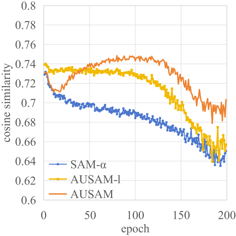
(b) WideResNet (${\nabla_{\mathbf{w}}}{L}(\mathbf{w})$)

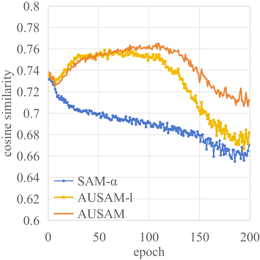
(c) PyramidNet (${\nabla_{\mathbf{w}}}{L}(\mathbf{w})$)

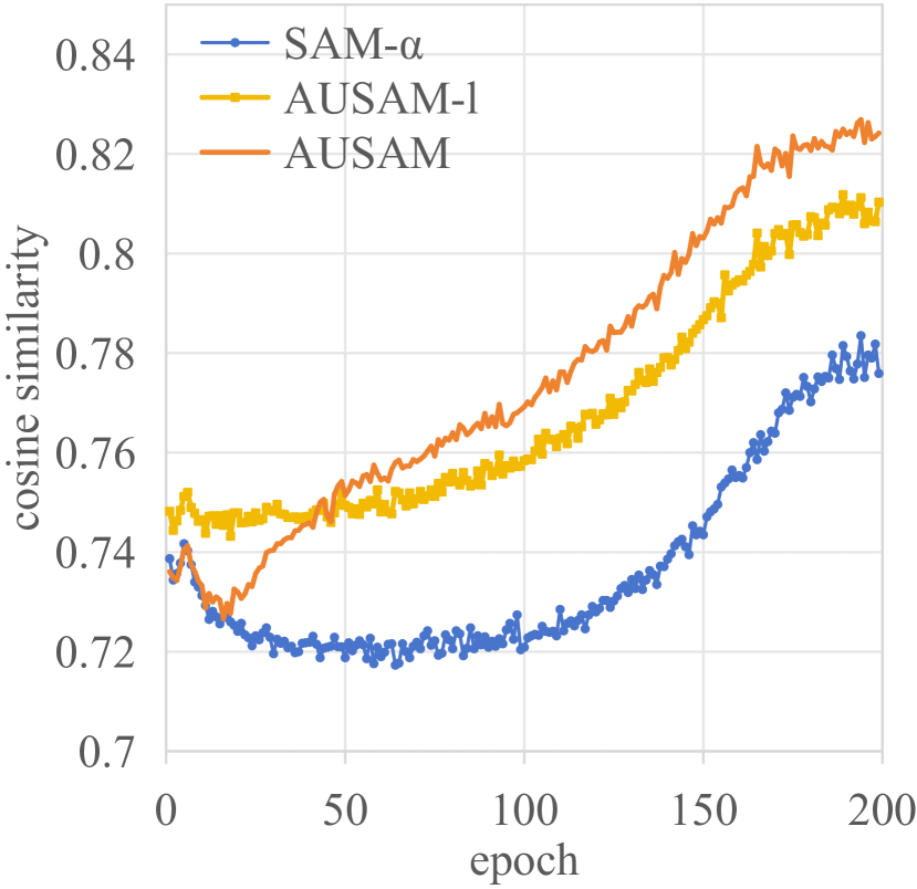
(d) Resnet-18 ($\nabla_{\mathbf{w}}{L}(\mathbf{w}+\bm{\varepsilon})$)

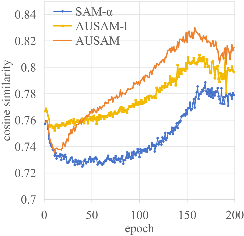
(e) WideResNet ($\nabla_{\mathbf{w}}{L}(\mathbf{w}+\bm{\varepsilon})$)

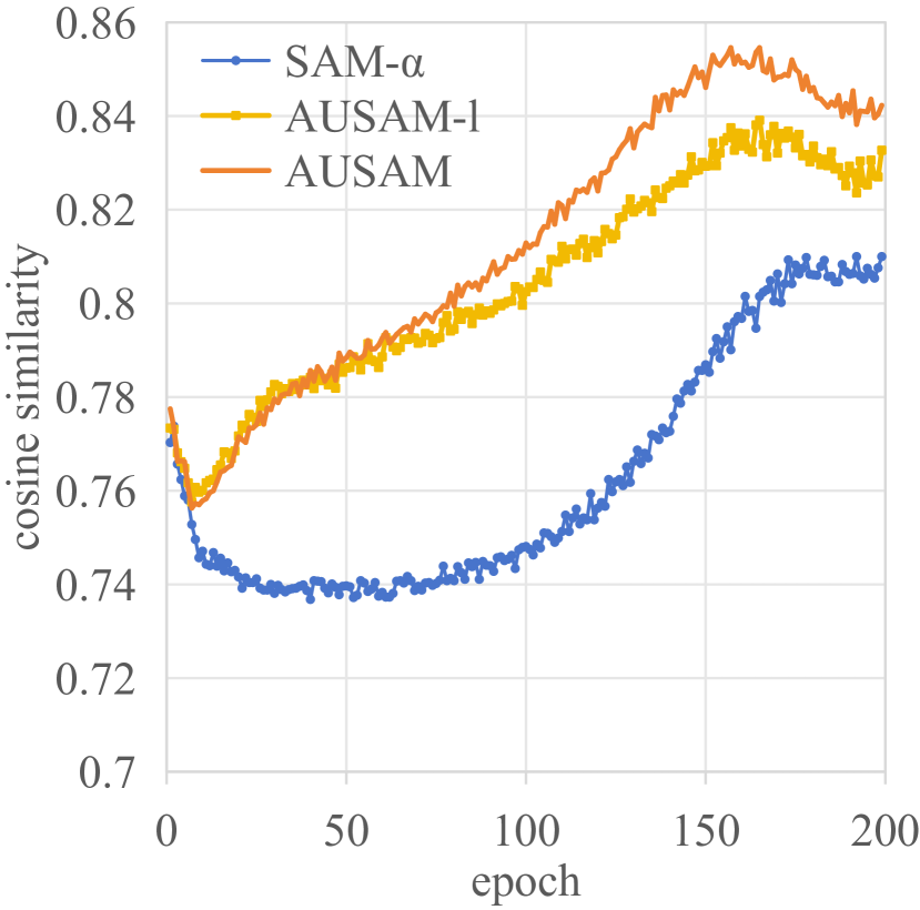
(f) PyramidNet ($\nabla_{\mathbf{w}}{L}(\mathbf{w}+\bm{\varepsilon})$)

Figure 1: The cosine similarity between the gradient of the sampled samples and the gradient of the whole mini-batch samples during training for the three different methods. The first row is the case when the perturbation is computed, and the second row is the case when the gradient descent is performed. The cosine similarity is higher when the averaged approach is used.

Appendix B Additional experiments

B.1 Approximate ability of Theorem 2

As shown in Fig. 1, we denote the method of randomly selecting $N$ samples from each mini-batch of size $K$ for training as SAM-$\alpha$ ($\alpha=N/K$). We optimize ResNet-18, WideResNet-28-10, and PyramidNet-110 on CIFAR-100 using SAM-$\alpha$, AUSAM-l, and AUSAM. We set $\alpha$ to 0.5 for SAM-$\alpha$ and AUSAM in this experiment.

During the training process, we calculate the cosine similarity between the gradients of the samples sampled by the three different methods and the gradients of the entire mini-batch samples, respectively. Fig. 1 illustrates that the cosine similarity of AUSAM is higher compared to that of SAM-$\alpha$ and AUSAM-l. This suggests that the gradient of the samples selected by AUSAM aligns more closely with the gradient direction of the entire mini-batch.

B.2 Asymptotic unbiased of gradient

In Fig. 3, we have plotted the average gradient of all batches in each epoch during training. This reflects the trend of gradient norms throughout the training process. As can be seen in Fig. 3, the gradient norm first increases and then decreases. Although the gradient norm has an upward process, we choose samples with larger gradient norm. This makes $(1-p_{\mathbf{x}}^{t})\left\|{{\nabla_{\mathbf{w}}}{L_{\mathbf{x}}}({\mathbf{w}_{t}})}\right\|$ smaller, the difference between the expected loss of full dataset and the expected loss of sampled subsets is even smaller. In the post-training phase, the gradient norm decreases gradually, which again makes this difference smaller, indicating that we AUSAM is progressively unbiased with training.

In Fig. 3, we have plotted the difference between the Perturbation Loss computed by the Full mini-batch(PLF) and the Perturbation Loss computed by the Sampled (PLS) samples. We find that in the initial stage of training, the perturbation loss of the sampled samples is larger than that of the whole mini-batch, which indicates that AUSAM can find larger perturbation loss in the local parameter region. With training, the difference between the perturbation loss of the sampled sample and the whole mini-batch is getting closer and closer to 0, indicating that our method is gradually getting closer to unbiased, which ensures that the gradient direction is consistent with the whole sample in the later stage of training and improves the accuracy of optimization.

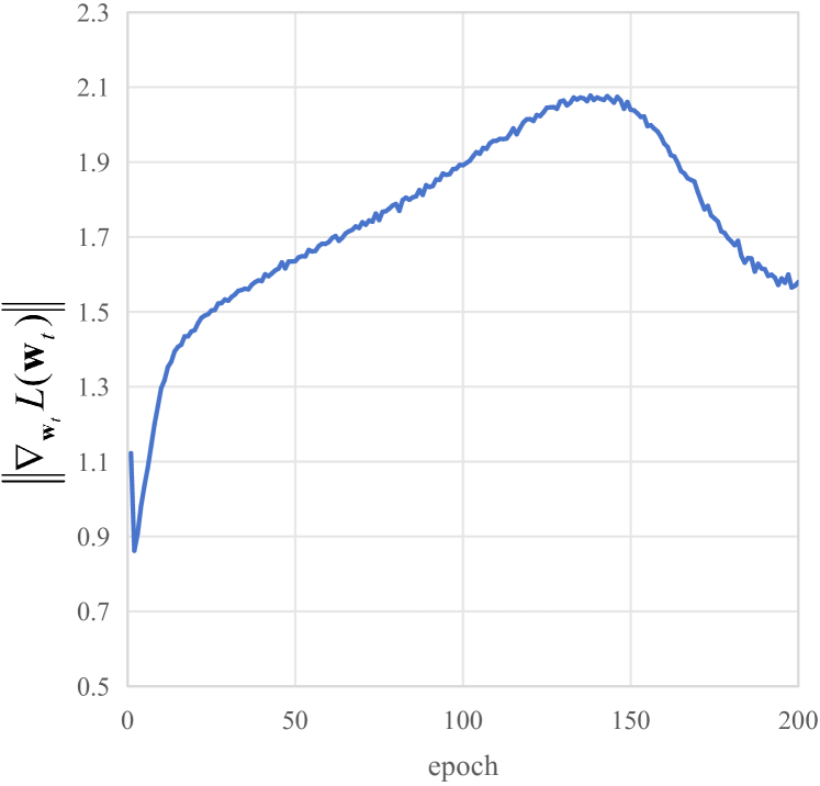
Figure 2: Trend of gradient norm throughout training.

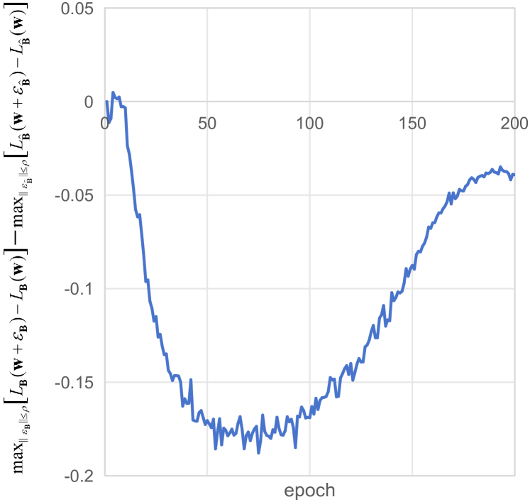
Figure 3: The difference between the Perturbation Loss computed by the Full mini-batch(PLF) and the Perturbation Loss computed by the Sampled (PLS) samples.

B.3 Application to Human Pose Estimation

SAM and AUSAM are applied to human pose estimation to show the utility of our method. The chosen method for human pose estimation is SimCC [24]. We conducted experiments on the MP$\mathrm{II}$ Human Pose dataset [1], which contains 40K person samples with 16 joints labels. We follow the evaluation procedure in [24], and conducted experiments with an image resolution of $224\times 224$. In the experiments, the base optimizer used for SAM and AUSAM is Adam, and the batch size is set to 64. We counted the time in seconds for each of them to be trained separately on the same device. The results are shown in Tab. 5.

Table 5: Results of training SimCC on MP$\mathrm{II}$ with Adam,SAM and AUSAM.

	Hea	Sho	Elb	Wri	Hip	Kne	Ank	Mean	Training time(s)
Adam	96.8	95.8	89.7	84.3	88.7	85.1	81.4	89.3	41889
SAM+Adam	97.0	95.7	89.6	84.2	88.4	85.5	81.9	89.4	76453
AUSAM+Adam	96.9	95.7	89.4	84.8	89.1	85.7	81.3	89.5	53081

It can be found that both SAM and AUSAM obtain better performance than the original Adam. In terms of speed, AUSAM is faster than SAM and slower than Adam. This indicates that AUSAM has a wide range of applicability.

B.4 Application to Quantization-Aware Training

We utilized SGD, SAM, and AUSAM to quantize the parameters of ResNet-18 and MobileNetv1 to W2A4 on the CIFAR-10 dataset, and the results are presented in Tab. 6. It can be observed that despite the reduction in time required for both forward and backward propagation after model quantization, AUSAM still manages to improve the optimization speed.

Table 6: Results of QAT with AUSAM on the Cifar-10.

	ResNet-18		MobileNets
Methods	Accuracy	Images/s	Accuracy	Images/s
Full prec.	88.72	\	85.81	\
QAT+SGD	88.86$\pm$0.18	1515(174%)	84.04$\pm$0.13	1244(153%)
QAT+SAM	89.75$\pm$0.21	870(100%)	84.72$\pm$0.11	816(100%)
QAT+AUSAM	89.63$\pm$0.10	1129(130%)	84.91$\pm$0.19	958(117%)

It can be observed that despite the reduction in time required for both forward and backward propagation after model quantization, AUSAM still manages to improve the optimization speed.

Appendix C Additional Analysis

C.1 Sampling leads to a large learning rate

Some studies have discussed the relationship between the generalization ability of models and batch size and learning rate. [20] uses experiments to show that the large-batch training leads to sharp local minima which have the poor generalization of SGD, while small-batches lead to flat minima which make SGD generalize well. [12] suggests that we should control the ratio of batch size to learning rate not too large while tuning the hyper-parameters. For AUSAM, by selecting a subset of samples from each mini-batch for training, it is equivalent to reducing the batch size. With the learning rate unchanged, a decrease in the ratio of batch size to learning rate contributes to maintaining the model’s generalization performance. In addition, the ratio of the gradient magnitude of the full mini-batch to the gradient magnitude of the selected sample can be expressed as follows:

$$\frac{{\|{\nabla_{\mathbf{w}}}L_{\mathbf{B}}^{SAM}(\mathbf{w})\|}}{{\|{\nabla_{\mathbf{w}}}L_{\hat{\mathbf{B}}}^{SAM}(\mathbf{w})\|}}\leq\alpha+(1-\alpha)\frac{{\|{\nabla_{\mathbf{w}}}L_{\check{\mathbf{B}}}^{SAM}(\mathbf{w})\|}}{{\|{\nabla_{\mathbf{w}}}L_{\hat{\mathbf{B}}}^{SAM}(\mathbf{w})\|}}.$$ (35)

Since we chose samples with $\|{\nabla_{\mathbf{w}}}L_{\hat{\mathbf{B}}}^{SAM}(\mathbf{w})\|\geq\|{\nabla_{\mathbf{w}}}L_{\tilde{\mathbf{B}}}^{SAM}(\mathbf{w})\|$ , then ${{\|{\nabla_{\mathbf{w}}}L_{B}^{SAM}(\mathbf{w})\|}}/{{\|{\nabla_{\mathbf{w}}}L_{\hat{\mathbf{B}}}^{SAM}(\mathbf{w})\|}}\leq 1$. This indicates that the selected samples provide a larger gradient for gradient descent, this contributes to faster gradient descent.

Proof.

Suppose we select $N$ data points from a mini-batch data $\mathbf{B}$ of size $K$, denoting them as $\mathbf{\hat{B}}$, and represent the remaining set of $M(M=K-N)$ data points as $\mathbf{\check{B}}$. The gradient over a mini-batch of data can be expressed as follow:

$${\nabla_{\mathbf{w}}}L_{\mathbf{B}}^{SAM}(\mathbf{w})=\frac{{\sum\limits_{i=1}^{M}{{\nabla_{\mathbf{w}}}L_{\check{B}_{i}}^{SAM}(\mathbf{w})}+\sum\limits_{j=1}^{N}{{\nabla_{\mathbf{w}}}L_{\hat{B}_{j}}^{SAM}(\mathbf{w})}}}{{M+N}}$$ (36)

$$=(1-\alpha){\nabla_{\mathbf{w}}}L_{\check{\mathbf{B}}}^{SAM}(\mathbf{w})+\alpha{\nabla_{\mathbf{w}}}L_{\hat{\mathbf{B}}}^{SAM}(\mathbf{w}),$$

where $\alpha=N/K$, ${\nabla_{\mathbf{w}}}L_{\check{\mathbf{B}}}^{SAM}(\mathbf{w})$ and ${\nabla_{\mathbf{w}}}L_{\hat{\mathbf{B}}}^{SAM}(\mathbf{w})$ are the average gradients computed through the data sets $\mathbf{\check{B}}$ and $\mathbf{\hat{B}}$, respectively.

Then, the ratio of the gradient norm for all the data in a mini-batch to the selected data is as follows:

$$\frac{{\|{\nabla_{\mathbf{w}}}L_{\mathbf{B}}^{SAM}(\mathbf{w})\|}}{{\|{\nabla_{\mathbf{w}}}L_{\mathbf{\hat{B}}}^{SAM}(\mathbf{w})\|}} =\frac{{\|(1-\alpha){\nabla_{\mathbf{w}}}L_{\mathbf{\check{B}}}^{SAM}(\mathbf{w})+\alpha{\nabla_{\mathbf{w}}}L_{\mathbf{\hat{B}}}^{SAM}(\mathbf{w})\|}}{{\|{\nabla_{\mathbf{w}}}L_{\mathbf{\hat{B}}}^{SAM}(\mathbf{w})\|}}$$ (37)

$$\leq\frac{{\|(1-\alpha){\nabla_{\mathbf{w}}}L_{\mathbf{\check{B}}}^{SAM}(\mathbf{w})\|+\|\alpha{\nabla_{\mathbf{w}}}L_{\mathbf{\hat{B}}}^{SAM}(\mathbf{w})\|}}{{\|{\nabla_{\mathbf{w}}}L_{\mathbf{\hat{B}}}^{SAM}(\mathbf{w})\|}}$$

$$=\alpha+(1-\alpha)\frac{{\|{\nabla_{\mathbf{w}}}L_{\mathbf{\check{B}}}^{SAM}(\mathbf{w})\|}}{{\|{\nabla_{\mathbf{w}}}L_{\mathbf{\hat{B}}}^{SAM}(\mathbf{w})\|}}.$$

Since we chose samples with ${\|{\nabla_{\mathbf{w}}}L_{\mathbf{\hat{B}}}^{SAM}(\mathbf{w})\|}\geq{\|{\nabla_{\mathbf{w}}}L_{\mathbf{\check{B}}}^{SAM}(\mathbf{w})\|}$, then $\frac{{\|{\nabla_{\mathbf{w}}}L_{\mathbf{B}}^{SAM}(\mathbf{w})\|}}{{\|{\nabla_{\mathbf{w}}}L_{\mathbf{\hat{B}}}^{SAM}(\mathbf{w})\|}}\leq 1$. ∎

Appendix D Hyperparameter

For CIFAR-10 and CIFAR-100, our hyperparameter settings are consistent. The exact training hyperparameters on CIFAR-10/100 and Tiny-ImageNet are reported in Tab. 7 and Tab. 8.

Table 7: Hyperparameters on Cifar-10/100.

Networks	Methods	Peak learning rate	Weight decay	$\rho$	$s_{max}$	$\alpha$
ResNet-18	SGD	0.05	0.001	\	\	\
	SAM			0.1	\	\
	AUSAM-0.5			0.1	0.5	0.5
	AUSAM-0.6			0.1	0.5	0.6
WideResNet-28-10	SGD	0.05	0.001	\	\	\
	SAM			0.1	\	\
	AUSAM-0.5			0.1	0.5	0.5
	AUSAM-0.6			0.1	0.5	0.6
PyramidNet-110	SGD	0.1	0.0005	\	\	\
	SAM			0.2	\	\
	AUSAM-0.5			0.2	1	0.5
	AUSAM-0.6			0.2	1	0.6

Table 8: Hyperparameters on Tiny-ImageNet.

Networks	Methods	Peak learning rate	Weight decay	$\rho$	$s_{max}$	$\alpha$
ResNet-18	SGD	0.05	0.001	\	\	\
	SAM			0.1	\	\
	AUSAM-0.5			0.1	0.5	0.5
	AUSAM-0.6			0.1	0.5	0.6
ResNet-50	SGD	0.1	0.0005	\	\	\
	SAM			0.1	\	\
	AUSAM-0.5			0.1	1	0.5
	AUSAM-0.6			0.1	1	0.6
MobileNetv1	SGD	0.05	0.0005	\	\	\
	SAM			0.05	\	\
	AUSAM-0.5			0.05	1	0.5
	AUSAM-0.6			0.05	1	0.6

When applying SAM and AUSAM to SimCC and QAT, we maintain most of the hyperparameter settings of SimCC and QAT, respectively. The partially changed hyperparameters are shown in Tab. 9 and Tab. 10, respectively.

Table 9: Hyperparameters settings for SimCC.

Methods	Batch size	Image size	learning rate	Weight decay	$\rho$	$s_{max}$
Adam	64	256$\times$256	0.001	0.0001	\	\
SAM+Adam					0.05	\
AUSAM+Adam					0.05	1

Table 10: Hyperparameters settings for QAT.

Networks	Methods	Batch size	Learning rate	Weight decay	$\rho$	$s_{max}$
ResNet-18	QAT+SGD	128	0.005	0.0005	\	\
	QATSAM				0.05	\
	QAT+AUSAM				0.05	0.5
MobileNetv1	QAT+SGD	128	0.005	0.0005	\	\
	QATSAM				0.05	\
	QAT+AUSAM				0.05	0.5

References

- [1] Mykhaylo Andriluka, Leonid Pishchulin, Peter Gehler, and Bernt Schiele. 2d human pose estimation: New benchmark and state of the art analysis. In IEEE Conference on Computer Vision and Pattern Recognition (CVPR), June 2014.
- [2] Maksym Andriushchenko and Nicolas Flammarion. Towards understanding sharpness-aware minimization. In Proceedings of the International Conference on Machine Learning (ICML), pages 639–668. PMLR, 2022.
- [3] Junbum Cha, Sanghyuk Chun, Kyungjae Lee, Han-Cheol Cho, Seunghyun Park, Yunsung Lee, and Sungrae Park. Swad: Domain generalization by seeking flat minima. Advances in Neural Information Processing Systems (NeurIPS), 34:22405–22418, 2021.
- [4] Patryk Chrabaszcz, Ilya Loshchilov, and Frank Hutter. A downsampled variant of imagenet as an alternative to the cifar datasets. arXiv preprint arXiv:1707.08819, 2017.
- [5] Jiaxin Deng, Junbiao Pang, Baochang Zhang, and Tian Wang. Effective gradient sample size via variation estimation for accelerating sharpness aware minimization. arXiv preprint arXiv:2403.08821, 2024.
- [6] Terrance DeVries and Graham W Taylor. Improved regularization of convolutional neural networks with cutout. arXiv preprint arXiv:1708.04552, 2017.
- [7] Jiawei Du, Hanshu Yan, Jiashi Feng, Joey Tianyi Zhou, Liangli Zhen, Rick Siow Mong Goh, and Vincent YF Tan. Efficient sharpness-aware minimization for improved training of neural networks. 2022.
- [8] Jiawei Du, Daquan Zhou, Jiashi Feng, Vincent Tan, and Joey Tianyi Zhou. Sharpness-aware training for free. Advances in Neural Information Processing Systems (NeurIPS), 35:23439–23451, 2022.
- [9] Steven K Esser, Jeffrey L McKinstry, Deepika Bablani, Rathinakumar Appuswamy, and Dharmendra S Modha. Learned step size quantization. In Proceedings of the International Conference on Learning Representations (ICLR), 2020.
- [10] Pierre Foret, Ariel Kleiner, Hossein Mobahi, and Behnam Neyshabur. Sharpness-aware minimization for efficiently improving generalization. 2021.
- [11] Dongyoon Han, Jiwhan Kim, and Junmo Kim. Deep pyramidal residual networks. In Proceedings of the Conference on Computer Vision and Pattern Recognition (CVPR), pages 5927–5935, 2017.
- [12] Fengxiang He, Tongliang Liu, and Dacheng Tao. Control batch size and learning rate to generalize well: Theoretical and empirical evidence. Advances in neural information processing systems, 32, 2019.
- [13] Kaiming He, Xiangyu Zhang, Shaoqing Ren, and Jian Sun. Deep residual learning for image recognition. In Proceedings of the Conference on Computer Vision and Pattern Recognition (CVPR), pages 770–778, 2016.
- [14] Sepp Hochreiter and Jürgen Schmidhuber. Simplifying neural nets by discovering flat minima. Advances in Neural Information Processing Systems (NeurIPS), 7, 1994.
- [15] Andrew G Howard, Menglong Zhu, Bo Chen, Dmitry Kalenichenko, Weijun Wang, Tobias Weyand, Marco Andreetto, and Hartwig Adam. Mobilenets: Efficient convolutional neural networks for mobile vision applications. arXiv preprint arXiv:1704.04861, 2017.
- [16] Pavel Izmailov, Dmitrii Podoprikhin, Timur Garipov, Dmitry Vetrov, and Andrew Gordon Wilson. Averaging weights leads to wider optima and better generalization. pages 876–885, 2018.
- [17] Benoit Jacob, Skirmantas Kligys, Bo Chen, Menglong Zhu, Matthew Tang, Andrew Howard, Hartwig Adam, and Dmitry Kalenichenko. Quantization and training of neural networks for efficient integer-arithmetic-only inference. In Proceedings of the Conference on Computer Vision and Pattern Recognition (CVPR), pages 2704–2713, 2018.
- [18] Weisen Jiang, Hansi Yang, Yu Zhang, and James Kwok. An adaptive policy to employ sharpness-aware minimization. In Proceedings of the International Conference on Learning Representations (ICLR), 2023.
- [19] Yiding Jiang, Behnam Neyshabur, Hossein Mobahi, Dilip Krishnan, and Samy Bengio. Fantastic generalization measures and where to find them. 2020.
- [20] Nitish Shirish Keskar, Dheevatsa Mudigere, Jorge Nocedal, Mikhail Smelyanskiy, and Ping Tak Peter Tang. On large-batch training for deep learning: Generalization gap and sharp minima. Proceedings of the International Conference on Learning Representations (ICLR), 2017.
- [21] Alex Krizhevsky, Geoffrey Hinton, et al. Learning multiple layers of features from tiny images. 2009.
- [22] Jungmin Kwon, Jeongseop Kim, Hyunseo Park, and In Kwon Choi. Asam: Adaptive sharpness-aware minimization for scale-invariant learning of deep neural networks. In Proceedings of the International Conference on Machine Learning (ICML), pages 5905–5914. PMLR, 2021.
- [23] Ya Le and Xuan Yang. Tiny imagenet visual recognition challenge. CS 231N, 7(7):3, 2015.
- [24] Yanjie Li, Sen Yang, Peidong Liu, Shoukui Zhang, Yunxiao Wang, Zhicheng Wang, Wankou Yang, and Shu-Tao Xia. Simcc: A simple coordinate classification perspective for human pose estimation. In European Conference on Computer Vision, pages 89–106. Springer, 2022.
- [25] Yong Liu, Siqi Mai, Xiangning Chen, Cho-Jui Hsieh, and Yang You. Towards efficient and scalable sharpness-aware minimization. In Proceedings of the Conference on Computer Vision and Pattern Recognition (CVPR), pages 12360–12370, 2022.
- [26] Ilya Loshchilov and Frank Hutter. Sgdr: Stochastic gradient descent with warm restarts. arXiv preprint arXiv:1608.03983, 2016.
- [27] Markus Nagel, Marios Fournarakis, Yelysei Bondarenko, and Tijmen Blankevoort. Overcoming oscillations in quantization-aware training. In Proceedings of the International Conference on Machine Learning (ICML), pages 16318–16330. PMLR, 2022.
- [28] Behnam Neyshabur, Srinadh Bhojanapalli, David McAllester, and Nati Srebro. Exploring generalization in deep learning. Advances in Neural Information Processing Systems (NeurIPS), 30, 2017.
- [29] Mansheej Paul, Surya Ganguli, and Gintare Karolina Dziugaite. Deep learning on a data diet: Finding important examples early in training. Advances in Neural Information Processing Systems, 34:20596–20607, 2021.
- [30] Ziheng Qin, Kai Wang, Zangwei Zheng, Jianyang Gu, Xiangyu Peng, Daquan Zhou, Lei Shang, Baigui Sun, Xuansong Xie, Yang You, et al. Infobatch: Lossless training speed up by unbiased dynamic data pruning. In Proceedings of the International Conference on Learning Representations (ICLR), 2024.
- [31] Ravi S Raju, Kyle Daruwalla, and Mikko Lipasti. Accelerating deep learning with dynamic data pruning. arXiv preprint arXiv:2111.12621, 2021.
- [32] Mariya Toneva, Alessandro Sordoni, Remi Tachet des Combes, Adam Trischler, Yoshua Bengio, and Geoffrey J Gordon. An empirical study of example forgetting during deep neural network learning. arXiv preprint arXiv:1812.05159, 2018.
- [33] Xiuying Wei, Ruihao Gong, Yuhang Li, Xianglong Liu, and Fengwei Yu. Qdrop: Randomly dropping quantization for extremely low-bit post-training quantization. In Proceedings of the International Conference on Learning Representations (ICLR), 2021.
- [34] Dongxian Wu, Shu-Tao Xia, and Yisen Wang. Adversarial weight perturbation helps robust generalization. Advances in Neural Information Processing Systems (NeurIPS), 33:2958–2969, 2020.
- [35] Sergey Zagoruyko and Nikos Komodakis. Wide residual networks. arXiv preprint arXiv:1605.07146, 2016.
- [36] Chiyuan Zhang, Samy Bengio, Moritz Hardt, Benjamin Recht, and Oriol Vinyals. Understanding deep learning requires rethinking generalization. 2017.
- [37] Chiyuan Zhang, Samy Bengio, Moritz Hardt, Benjamin Recht, and Oriol Vinyals. Understanding deep learning (still) requires rethinking generalization. Communications of the ACM, 64(3):107–115, 2021.
- [38] Xingxuan Zhang, Renzhe Xu, Han Yu, Yancheng Dong, Pengfei Tian, and Peng Cui. Flatness-aware minimization for domain generalization. In Proceedings of the International Conference on Computer Vision (ICCV), pages 5189–5202, 2023.
- [39] Juntang Zhuang, Boqing Gong, Liangzhe Yuan, Yin Cui, Hartwig Adam, Nicha Dvornek, Sekhar Tatikonda, James Duncan, and Ting Liu. Surrogate gap minimization improves sharpness-aware training. 2022.