On Siegel results about the zeros of the auxiliary function of Riemann.

Abstract.

We state and give complete proof of the results of Siegel about the zeros of the auxiliary function of Riemann $\mathop{\mathcal{R}}\nolimits(s)$. We point out the importance of the determination of the limit to the left of the zeros of $\mathop{\mathcal{R}}\nolimits(s)$ with positive imaginary part, obtaining the term $-\sqrt{T/2\pi}P(\sqrt{T/2\pi})$ that would explain the periodic behaviour observed with the statistical study of the zeros of $\mathop{\mathcal{R}}(s)$.

We precise also the connection of the position on the zeros of $\mathop{\mathcal{R}}\nolimits(s)$ with the zeros of $\zeta(s)$ in the critical line.

1. Introduction

In his paper [14] Riemann asserts to have proved that all but an infinitesimal proportion of zeros of zeta are in the critical line. This is repeated in a letter to Weierstrass [15]*p. 823–825, where he says that the difficult proof depends on a new development of $\Xi(t)$ that he has not simplified sufficiently to communicate. The Riemann-Siegel expansion for $\zeta(s)$ were recovered by Siegel from Riemann’s papers. Siegel in his publication [17] concluded that in Riemann’s Nachlass there is no approach to the proof of his assertion on the real zeros of $\Xi(t)$. However, Siegel connected the zeros of the new function $\mathop{\mathcal{R}}\nolimits(s)$, found in Riemann’s papers, with the zeros of $\zeta(s)$. The main objective of this paper is to expose and give a complete proof of the results of Siegel on the zeros of $\mathop{\mathcal{R}}\nolimits(s)$.

Siegel [17] proved an asymptotic expression (16) valid for $1-\sigma\geq t^{a}$ with $a=\frac{3}{7}$. He claims that we may prove this with $a=\varepsilon$ for any $\varepsilon>0$. In [4]*Th. 11 we proved it for $1-\sigma\geq t^{2/5}\log t$. In this paper, it will be desirable to have proved the claim with $a<\frac{1}{3}$ so that the term in $|\sigma|^{3/2}=\mathop{\hbox{\cmmib o}}\nolimits(t^{1/2})$. For this reason we will keep $a$ undetermined, to see the possible consequences of the hypothesis of being $a<\frac{1}{3}$. On the other hand, we may assume in all our results that $a=\frac{3}{7}$ as done by Siegel (see also [7]*Th. 9).

The paper contains many computations that Siegel does not detail. First, we state three main Theorems in Section 2. We postpone its proof, and in Section 3 we give the main applications to the zeros of $\mathop{\mathcal{R}}\nolimits(s)$. We note that in [9] we have given a better result about the number of zeros than the one obtained by Siegel methods (see Remark 5). Our corollary 11 slightly improves on Siegel’s results. This corollary implies that $\mathop{\mathcal{R}}\nolimits(s)$ contains at least $>cT$ zeros to the left of the critical line, with $c=35/198\pi$. This constant is a slight improvement over the one in Siegel, in any case it is a very poor result, as it only shows that the number of zeros of $\zeta(s)$ on the critical line $N_{0}(T)$ is greater than $cT$. Our computation of the zeros of $\mathop{\mathcal{R}}\nolimits(s)$ [2] makes plausible that $\frac{2}{3}$ of the zeros of $\mathop{\mathcal{R}}\nolimits(s)$ are on the left of the critical line, this would imply that $2/3$ of the zeros of $\zeta(s)$ will be simple zeros on the critical line.

In Section 5 we prove Theorem 3. It is in Siegel only implicitly. In Section 7 we prove Theorem 1. We make a modification of Siegel’s reasoning. He uses a function $g(s)=\pi^{-(s+1)/2}e^{-\pi is/4}\Gamma(\frac{s+1}{2})\mathop{\mathcal{R}}\nolimits(s)$, while we use $F(s)=s\pi^{-s/2}\Gamma(s/2)\mathop{\mathcal{R}}\nolimits(s)$. The main advantage is that our function is entire, while $g(s)$ has poles and zeros at the negative real axis, making the Siegel reasoning difficult. We postpone for section 8 the proof of propositions 20 and 21 that are mere computations.

1.1. Notations

We use $N(\beta\leq\sigma,T)$ and $N(\beta>\sigma,T)$ to denote the count of zeros $\rho=\beta+i\gamma$ of $\mathop{\mathcal{R}}\nolimits(s)$ contained in $(-\infty,\sigma]\times(0,T]$ and $(\sigma,+\infty)\times(0,T]$ respectively counting with multiplicities. The sum of the two is denoted by $N_{\mathop{\mathcal{R}}\nolimits}(T)$. $N(T)$ and $N_{0}(T)$ denote the number of zeros of $\zeta(s)$ on the critical strip and in the critical line, respectively, as usual. We use $\mathop{\hbox{\cmbsy O}}\nolimits^{*}(h)$ to denote a quantity $R$ bounded by $|R|\leq|h|$.

2. Main Results.

Applying Littlewood’s lemma to $\mathop{\mathcal{R}}\nolimits(s)$ in the rectangle $[\sigma,4]\times[t_{0},T]$ yields

Theorem 1.

Let $1\leq t_{0}$ and $\sigma\leq 1$ be fixed, then for $T\to+\infty$

(1) $$\int_{t_{0}}^{T}\log|\mathop{\mathcal{R}}\nolimits(\sigma+it)|\,dt=2\pi\sum_{\begin{subarray}{c}\beta>\sigma\\ 0<\gamma\leq T\end{subarray}}(\beta-\sigma)+\mathop{\hbox{\cmbsy O}}\nolimits_{\sigma}(\log T).$$

With the combed function $s\pi^{-s/2}\Gamma(s/2)\mathop{\mathcal{R}}\nolimits(s)$, we can apply Littlewood’s lemma on the rectangle $[\sigma_{0},\sigma]\times[t_{0},T]$ to get

Theorem 2.

Let $1\leq t_{0}$ and $\sigma\leq 10$ fixed, then for $T\to+\infty$ we have

(2) $$2\pi\sum_{\begin{subarray}{c}\beta\leq\sigma\\ 0<\gamma\leq T\end{subarray}}(\sigma-\beta)=\sigma\Bigl{(}\frac{T}{2}\log\frac{T}{2\pi}-\frac{T}{2}\Bigr{)}+\frac{T}{2}\log 2+\int_{t_{0}}^{T}\log|\mathop{\mathcal{R}}\nolimits(\sigma+it)|\,dt+\mathop{\hbox{\cmbsy O}}\nolimits_{\sigma}(T^{20/21}).$$

In some cases, we have independent information on the integral of $\log|\mathop{\mathcal{R}}\nolimits(\sigma+t)|$:

Theorem 3.

Given $\sigma_{1}>3$, there is a constant $C$ such that for $\sigma\geq\sigma_{1}$ and $1\leq t_{0}<T$ we have

(3) $$\Bigl{|}\int_{t_{0}}^{T}\log|\mathop{\mathcal{R}}\nolimits(\sigma+it)|\,dt\Bigr{|}\leq C2^{-\sigma}.$$

3. Applications of the main Theorems

Proposition 4.

The number of zeros $\rho=\beta+i\gamma$ of $\mathop{\mathcal{R}}\nolimits(s)$ with $0<\gamma<T$ is

(4) $$N_{\mathop{\mathcal{R}}\nolimits}(T)=\frac{T}{4\pi}\log\frac{T}{2\pi}-\frac{T}{4\pi}+\mathop{\hbox{\cmbsy O}}\nolimits(T^{20/21}).$$

Proof.

By Theorems 2 and 3 we have for $\sigma=4$ and $\sigma=5$ for $T\to+\infty$

(5) $$2\pi\sum_{\begin{subarray}{c}\beta\leq\sigma\\ 0<\gamma\leq T\end{subarray}}(\sigma-\beta)=\sigma\Bigl{(}\frac{T}{2}\log\frac{T}{2\pi}-\frac{T}{2}\Bigr{)}+\frac{T}{2}\log 2+\mathop{\hbox{\cmbsy O}}\nolimits(T^{20/21}).$$

Except for a finite number, the zeros of $\mathop{\mathcal{R}}\nolimits(s)$ with $\gamma>0$ satisfies $\beta\leq 3$ as shown in [5]*Cor. 14. Hence

$$N_{\mathop{\mathcal{R}}\nolimits}(T)=\sum_{\begin{subarray}{c}\beta\leq 5\\ 0<\gamma\leq T\end{subarray}}(5-\beta)-\sum_{\begin{subarray}{c}\beta\leq 4\\ 0<\gamma\leq T\end{subarray}}(4-\beta)+\mathop{\hbox{\cmbsy O}}\nolimits(1).$$

The result is obtained by subtracting the above results. ∎

Remark 5.

By a different and more direct reasoning, we have proved in [9] the more precise result

$$N_{\mathop{\mathcal{R}}\nolimits}(T)=\frac{T}{4\pi}\log\frac{T}{2\pi}-\frac{T}{4\pi}-\frac{1}{2}\sqrt{\frac{T}{2\pi}}+\mathop{\hbox{\cmbsy O}}\nolimits(T^{2/5}\log T).$$

Proposition 6.

For $T\to+\infty$ and denoting by $\rho=\beta+i\gamma$ the zeros of $\mathop{\mathcal{R}}\nolimits(s)$, we have

(6) $$\sum_{0<\gamma\leq T}\beta=-\frac{T}{4\pi}\log 2+\mathop{\hbox{\cmbsy O}}\nolimits(T^{20/21}).$$

Proof.

For $\sigma=4$, for example, we have

$$\sum_{\begin{subarray}{c}\beta\leq 4\\ 0<\gamma\leq T\end{subarray}}(\sigma-\beta)=\sigma N_{\mathop{\mathcal{R}}\nolimits}(T)-\sum_{0<\gamma\leq T}\beta=\sigma\Bigl{(}\frac{T}{4\pi}\log\frac{T}{2\pi}-\frac{T}{4\pi}\Bigr{)}-\sum_{0<\gamma\leq T}\beta+\mathop{\hbox{\cmbsy O}}\nolimits(T^{20/21}).$$

Comparing with (5) we get our result. ∎

Lemma 7.

Let $\sigma^{\prime}<\sigma\leq 10$ then

(7) $$(\sigma-\sigma^{\prime})N(\beta\leq\sigma,T) \geq(\sigma-\sigma^{\prime})\Bigl{(}\frac{T}{4\pi}\log\frac{T}{2\pi}-\frac{T}{4\pi}\Bigr{)}+$$

$$+\frac{1}{2\pi}\int_{t_{0}}^{T}\log|\mathop{\mathcal{R}}\nolimits(\sigma+it)|\,dt-\frac{1}{2\pi}\int_{t_{0}}^{T}\log|\mathop{\mathcal{R}}\nolimits(\sigma^{\prime}+it)|\,dt+\mathop{\hbox{\cmmib o}}\nolimits(T).$$

Proof.

by Theorem 2 we have

$$\sum_{\begin{subarray}{c}\beta\leq\sigma\\ 0<\gamma\leq T\end{subarray}}(\sigma-\beta) =\sigma\Bigl{(}\frac{T}{4\pi}\log\frac{T}{2\pi}-\frac{T}{4\pi}\Bigr{)}+\frac{T\log 2}{4\pi}+\frac{1}{2\pi}\int_{t_{0}}^{T}\log|\mathop{\mathcal{R}}\nolimits(\sigma+it)|\,dt+\mathop{\hbox{\cmmib o}}\nolimits(T),$$

$$\sum_{\begin{subarray}{c}\beta\leq\sigma^{\prime}\\ 0<\gamma\leq T\end{subarray}}(\sigma^{\prime}-\beta) =\sigma^{\prime}\Bigl{(}\frac{T}{4\pi}\log\frac{T}{2\pi}-\frac{T}{4\pi}\Bigr{)}+\frac{T\log 2}{4\pi}+\frac{1}{2\pi}\int_{t_{0}}^{T}\log|\mathop{\mathcal{R}}\nolimits(\sigma^{\prime}+it)|\,dt+\mathop{\hbox{\cmmib o}}\nolimits(T).$$

We subtract the two equations. Since $\sigma^{\prime}<\sigma$ we have

$$\sum_{\begin{subarray}{c}\beta\leq\sigma\\ 0<\gamma\leq T\end{subarray}}(\sigma-\beta)-\sum_{\begin{subarray}{c}\beta\leq\sigma^{\prime}\\ 0<\gamma\leq T\end{subarray}}(\sigma^{\prime}-\beta)=\sum_{\begin{subarray}{c}\beta\leq\sigma\\ 0<\gamma\leq T\end{subarray}}(\sigma-\beta)-\sum_{\begin{subarray}{c}\beta\leq\sigma\\ 0<\gamma\leq T\end{subarray}}(\sigma^{\prime}-\beta)+\sum_{\begin{subarray}{c}\sigma^{\prime}<\beta\leq\sigma\\ 0<\gamma\leq T\end{subarray}}(\sigma^{\prime}-\beta)$$

$$=(\sigma-\sigma^{\prime})N(\beta\leq\sigma,T)+\sum_{\begin{subarray}{c}\sigma^{\prime}<\beta\leq\sigma\\ 0<\gamma\leq T\end{subarray}}(\sigma^{\prime}-\beta)\leq(\sigma-\sigma^{\prime})N(\beta\leq\sigma,T).$$

Therefore,

$$(\sigma-\sigma^{\prime})N(\beta\leq\sigma,T) \geq(\sigma-\sigma^{\prime})\Bigl{(}\frac{T}{4\pi}\log\frac{T}{2\pi}-\frac{T}{4\pi}\Bigr{)}+\frac{1}{2\pi}\int_{t_{0}}^{T}\log|\mathop{\mathcal{R}}\nolimits(\sigma+it)|\,dt$$

$$-\frac{1}{2\pi}\int_{t_{0}}^{T}\log|\mathop{\mathcal{R}}\nolimits(\sigma^{\prime}+it)|\,dt+\mathop{\hbox{\cmmib o}}\nolimits(T).\qed$$

Lemma 8.

For $\sigma^{\prime}<\sigma\leq 10$ we have

(8) $$(\sigma-\sigma^{\prime})N(\beta\leq\sigma,T)\geq(\sigma-\sigma^{\prime})\Bigl{(}\frac{T}{4\pi}\log\frac{T}{2\pi}-\frac{T}{4\pi}\Bigr{)}-\frac{1}{2\pi}\int_{t_{0}}^{T}\log|\mathop{\mathcal{R}}\nolimits(\sigma^{\prime}+it)|\,dt+\mathop{\hbox{\cmmib o}}\nolimits(T).$$

Proof.

By Lemma 7 and Theorem 1 we have for any $\sigma^{\prime\prime}$ with $\sigma>\sigma^{\prime\prime}>\sigma^{\prime}$

$$(\sigma^{\prime\prime}-\sigma^{\prime})N(\beta\leq\sigma,T) \geq(\sigma^{\prime\prime}-\sigma^{\prime})\Bigl{(}\frac{T}{4\pi}\log\frac{T}{2\pi}-\frac{T}{4\pi}\Bigr{)}+\sum_{\begin{subarray}{c}\beta>\sigma^{\prime\prime}\\ 0<\gamma\leq T\end{subarray}}(\beta-\sigma^{\prime\prime})$$

$$-\frac{1}{2\pi}\int_{t_{0}}^{T}\log|\mathop{\mathcal{R}}\nolimits(\sigma^{\prime}+it)|\,dt+\mathop{\hbox{\cmmib o}}\nolimits(T).$$

We have (by Proposition 4)

$$\sum_{\begin{subarray}{c}\beta>\sigma^{\prime\prime}\\ 0<\gamma\leq T\end{subarray}}(\beta-\sigma^{\prime\prime})\geq\sum_{\begin{subarray}{c}\beta>\sigma\\ 0<\gamma\leq T\end{subarray}}(\beta-\sigma^{\prime\prime})\geq(\sigma-\sigma^{\prime\prime})N(\beta>\sigma,T)$$

$$=(\sigma-\sigma^{\prime\prime})\Bigl{(}\frac{T}{4\pi}\log\frac{T}{2\pi}-\frac{T}{4\pi}-N(\beta\leq\sigma,T)+\mathop{\hbox{\cmmib o}}\nolimits(T)\Bigr{)}.$$

Therefore,

$$(\sigma^{\prime\prime}-\sigma^{\prime})N(\beta\leq\sigma,T) +(\sigma-\sigma^{\prime\prime})N(\beta\leq\sigma,T)$$

$$\geq(\sigma-\sigma^{\prime})\Bigl{(}\frac{T}{4\pi}\log\frac{T}{2\pi}-\frac{T}{4\pi}\Bigr{)}-\frac{1}{2\pi}\int_{t_{0}}^{T}\log|\mathop{\mathcal{R}}\nolimits(\sigma^{\prime}+it)|\,dt+\mathop{\hbox{\cmmib o}}\nolimits(T).\qed$$

Lemma 9.

Let $f\colon[0,+\infty)\to\mathbf{C}$ integrable on any compact set and such that

$$\lim_{T\to+\infty}\frac{1}{T}\int_{0}^{T}|f(t)|^{2}\,dt=+\infty.$$

Given $t_{0}$ there is some $T_{0}$ such that for $T\geq T_{0}$ we have

(9) $$\int_{t_{0}}^{T}\log|f(t)|\,dt\leq\frac{T}{2}\log\Bigl{(}\frac{1}{T}\int_{0}^{T}|f(t)|^{2}\,dt\Bigr{)}.$$

Proof.

Since $\log x$ is a concave function by Jensen’s inequality [16]*p. 61 for $T>t_{0}$ we have

$$\frac{1}{T-t_{0}}\int_{t_{0}}^{T}\log|f(t)|^{2}\,dt\leq\log\Bigl{(}\frac{1}{T-t_{0}}\int_{t_{0}}^{T}|f(t)|^{2}\,dt\Bigr{)}.$$

Let us define

$$A:=\int_{t_{0}}^{T}|f(t)|^{2}\,dt\leq B:=\int_{0}^{T}|f(t)|^{2}\,dt.$$

The function $x\mapsto\frac{x}{2}\log\frac{B}{x}$ is increasing for $x\in[T-t_{0},T]$, since the derivative is $\frac{1}{2}\log\frac{B}{x}-\frac{1}{2}$, which is positive for $B>ex$. So, we only need that $B>eT$ and this happens for $T\geq T_{0}$ by hypothesis. Then

$$\int_{t_{0}}^{T}\log|f(t)|\,dt\leq\frac{T-t_{0}}{2}\log\frac{A}{T-t_{0}}\leq\frac{T-t_{0}}{2}\log\frac{B}{T-t_{0}}\leq\frac{T}{2}\log\frac{B}{T}.$$

This is our inequality. ∎

Proposition 10.

There is some $T_{0}$ such that for $T>T_{0}$ we have

(10) $$N(\beta\leq\tfrac{1}{2},T)\geq\frac{35T}{396\pi}+\frac{5}{11\pi}\int_{t_{0}}^{T}\log|\mathop{\mathcal{R}}\nolimits(\tfrac{1}{2}+it)|\,dt.$$

Proof.

Applying Lemma 7 with $\sigma=1/2$ and $\sigma^{\prime}<1/2$ yields

$$(\tfrac{1}{2}-\sigma^{\prime})N(\beta\leq\tfrac{1}{2},T) \geq(\tfrac{1}{2}-\sigma^{\prime})\Bigl{(}\frac{T}{4\pi}\log\frac{T}{2\pi}-\frac{T}{4\pi}\Bigr{)}+$$

$$+\frac{1}{2\pi}\int_{t_{0}}^{T}\log|\mathop{\mathcal{R}}\nolimits(\tfrac{1}{2}+it)|\,dt-\frac{1}{2\pi}\int_{t_{0}}^{T}\log|\mathop{\mathcal{R}}\nolimits(\sigma^{\prime}+it)|\,dt+\mathop{\hbox{\cmmib o}}\nolimits(T).$$

In [8] we proved that for $\sigma^{\prime}\leq 1/4$ we have

$$\frac{1}{T}\int_{0}^{T}|\mathop{\mathcal{R}}\nolimits(\sigma^{\prime}+it)|^{2}\,dt=\frac{2}{(1-2\sigma^{\prime})(3-2\sigma^{\prime})}\Bigl{(}\frac{T}{2\pi}\Bigr{)}^{\frac{1}{2}-\sigma^{\prime}}+\mathop{\hbox{\cmbsy O}}\nolimits(T^{\frac{1}{4}-\sigma^{\prime}}).$$

This and Lemma 9 yields for $\sigma\leq 1/4$ and $T$ big enough

$$\int_{t_{0}}^{T}\log|\mathop{\mathcal{R}}\nolimits(\sigma^{\prime}+it)|\,dt\leq(\tfrac{1}{2}-\sigma^{\prime})\frac{T}{2}\log\frac{T}{2\pi}-\frac{T}{2}\log\frac{(1-2\sigma^{\prime})(3-2\sigma^{\prime})}{2}+\mathop{\hbox{\cmbsy O}}\nolimits(T^{3/4}).$$

Hence,

$$(\tfrac{1}{2}-\sigma^{\prime})N(\beta\leq\tfrac{1}{2},T) \geq-(\tfrac{1}{2}-\sigma^{\prime})\frac{T}{4\pi}+$$

$$+\frac{1}{2\pi}\int_{t_{0}}^{T}\log|\mathop{\mathcal{R}}\nolimits(\tfrac{1}{2}+it)|\,dt+\frac{T}{4\pi}\log\frac{(1-2\sigma^{\prime})(3-2\sigma^{\prime})}{2}+\mathop{\hbox{\cmmib o}}\nolimits(T).$$

The function

$$f(\sigma^{\prime})=-1+\frac{1}{\frac{1}{2}-\sigma^{\prime}}\log\frac{(1-2\sigma^{\prime})(3-2\sigma^{\prime})}{2},$$

has a maximum near $\sigma^{\prime}=-3/5$ where $f(-3/5)>7/18$. Therefore, taking $\sigma^{\prime}=-3/5$ we get

$$\frac{11}{10}N(\beta\leq\tfrac{1}{2},T)\geq\frac{7T}{72\pi}+\frac{1}{2\pi}\int_{t_{0}}^{T}\log|\mathop{\mathcal{R}}\nolimits(\tfrac{1}{2}+it)|\,dt+\mathop{\hbox{\cmmib o}}\nolimits(T).$$

Since $f(-3/5)>7/18$ the term $\mathop{\hbox{\cmmib o}}\nolimits(T)$ can be eliminated for $T\geq T_{0}$, taking $T_{0}$ big enough. ∎

Corollary 11.

There exists some $T_{0}$ such that for $T\geq T_{0}$ we have

$$N(\beta\leq\tfrac{1}{2},T)\geq\frac{35T}{396\pi}+\frac{5}{11}\sum_{\begin{subarray}{c}\beta>1/2\\ 0<\gamma\leq T\end{subarray}}(\beta-\tfrac{1}{2}).$$

Proof.

In Proposition 10 substitute the integral by its value in Theorem 1. The error term $\mathop{\hbox{\cmbsy O}}\nolimits(\log T)$ is eliminated due to the strict inequality $f(-3/5)>7/18$. ∎

4. Connection with the zeros of $\zeta(s)$

We have $\zeta(\frac{1}{2}+it)=e^{-i\vartheta(t)}Z(t)$ where $\vartheta(t)$ and $Z(t)$ are real analytic functions. These are connected to $\mathop{\mathcal{R}}\nolimits(s)$ by

$$Z(t)=2\mathop{\mathrm{Re}}\nolimits\bigl{\{}e^{i\vartheta(t)}\mathop{\mathcal{R}}\nolimits(\tfrac{1}{2}+it)\bigr{\}},$$

(see [1]). In [10] we show that $\mathop{\mathcal{R}}\nolimits(\frac{1}{2}+it)=e^{-i\omega(t)}g(t)$ where $\omega(t)$ and $g(t)$ are real analytic functions. It follows that a point $\frac{1}{2}+it$ with $t\in\mathbf{R}$ is a zero of $\zeta(s)$ if and only if it is a zero of $\mathop{\mathcal{R}}\nolimits(s)$ or if

$$\cos\bigl{(}\vartheta(t)-\omega(t)\bigr{)}=0.$$

Also, it is shown in [10] that for $T>0$ we have

$$\omega(T)=2\pi N(\beta\geq 1/2,T)+\mathop{\hbox{\cmbsy O}}\nolimits(\log T).$$

If there were no zeros to the right of the critical line, $N(\beta\geq 1/2,T)=0$, then the function $\vartheta(t)-\omega(t)$ will increase for $t\in[0,T]$ from $0$ to $\approx\vartheta(T)$ and the number of zeros of $\zeta(s)$ in the critical line from $t=0$ to $t=T$ will be $\vartheta(T)/\pi$. Almost all zeros of the zeta function will be on the critical line. But this does not appear to be true, our (limited) computation of zeros [2] points to the approximate equality $N(\beta\geq 1/2,T)\approx\vartheta(T)/6\pi$.

5. Proof of Theorem 3

Lemma 12.

For $s=\sigma+it$ with $\sigma\geq 2$, $t\geq 0$ and $|s|>2\pi e^{2}$ we have

(11) $$\mathop{\mathcal{R}}\nolimits(s)=\zeta(s)(1+W(s)),\qquad|W(s)|\leq C\Bigl{(}\frac{|s|}{2\pi e}\Bigr{)}^{\frac{1-\sigma}{2}},$$

where $C$ is an absolute constant.

Proof.

In [5]*Thm. 12 it is proved that for $s=\sigma+it$ with $t>0$, $\sigma>0$ and such that $|s|>2\pi e^{2}$ we have

$$\mathop{\mathcal{R}}\nolimits(s)=\sum_{n=1}^{\ell}\frac{1}{n^{s}}+R(s),\qquad|R(s)|\leq C|s/2\pi e|^{-\sigma/2},$$

where, $\xi=\sqrt{\frac{s}{2\pi i}}=\xi_{1}+i\xi_{2}$ with $0<-\xi_{2}<\xi_{1}$ and $\ell=\lfloor\xi_{1}-\xi_{2}\rfloor$, and $C$ is an absolute constant.

Therefore, under these conditions, but assuming $\sigma>1$

$$\mathop{\mathcal{R}}\nolimits(s)=\zeta(s)-\sum_{n=\ell+1}^{\infty}\frac{1}{n^{s}}+R(s).$$

Notice that $|\xi_{1}|=\xi_{1}$ and $|\xi_{2}|=-\xi_{2}$, so that

$$|\xi|-1\leq|\xi_{1}|+|\xi_{2}|-1<\ell=\lfloor\xi_{1}-\xi_{2}\rfloor\leq|\xi_{1}|+|\xi_{2}|\leq\sqrt{2}|\xi|=\sqrt{|s|/\pi}.$$

Therefore,

$$\Bigl{|}\sum_{n=\ell+1}^{\infty}\frac{1}{n^{s}}\Bigr{|}\leq\sum_{n>|\xi|}\frac{1}{n^{\sigma}}\leq|\xi|^{-\sigma}+\int_{|\xi|}^{\infty}x^{-\sigma}\,dx=(|s|/2\pi)^{-\sigma/2}+\frac{1}{\sigma-1}(|s|/2\pi)^{(1-\sigma)/2}.$$

It follows that for $\sigma\geq 2$

$$\Bigl{|}R(s)-\sum_{n=\ell+1}^{\infty}\frac{1}{n^{s}}\Bigr{|}\leq C|s/2\pi e|^{-\sigma/2}+(|s|/2\pi)^{-\sigma/2}+\frac{1}{\sigma-1}(|s|/2\pi)^{(1-\sigma)/2}\leq C|s/2\pi e|^{(1-\sigma)/2}.$$

Therefore,

$$\mathop{\mathcal{R}}\nolimits(s)=\zeta(s)+V(s)=\zeta(s)(1+W(s)),\qquad|W(s)|\leq C\zeta(2)|s/2\pi e|^{(1-\sigma)/2}.\qed$$

Proposition 13.

There exist $\sigma_{0}>3$, $t_{0}>1$ and a constant $C$ such that for $T>t_{0}$ and $\sigma>\sigma_{0}$, we have

(12) $$\Bigl{|}\int_{t_{0}}^{T}\log|\mathop{\mathcal{R}}\nolimits(\sigma+it)|\,dt\Bigr{|}\leq C2^{-\sigma},$$

Proof.

We have

$$\int_{t_{0}}^{T}\log|\mathop{\mathcal{R}}\nolimits(\sigma+it)|\,dt=\int_{t_{0}}^{T}\log|\zeta(\sigma+it)|\,dt+\int_{t_{0}}^{T}|\log(1+W(\sigma+it))|\,dt.$$

The integral in the zeta function is treated easily

$$\int_{t_{0}}^{T}\log|\zeta(\sigma+it)|\,dt =\mathop{\mathrm{Re}}\nolimits\int_{t_{0}}^{T}\sum_{n=2}^{\infty}\frac{\Lambda(n)}{\log n}\frac{1}{n^{s}}\,dt=\int_{t_{0}}^{T}\sum_{n=2}^{\infty}\frac{\Lambda(n)}{\log n}\frac{\cos(t\log n)}{n^{\sigma}}\,dt$$

$$=\sum_{n=2}^{\infty}\frac{\Lambda(n)}{\log n}\frac{\sin(T\log n)-\sin(t_{0}\log n)}{n^{\sigma}\log n}.$$

So, in absolute value

$$\Bigl{|}\int_{t_{0}}^{T}\log|\zeta(\sigma+it)|\,dt\Bigr{|}\leq 2^{-\sigma}\sum_{n=2}^{\infty}\frac{2\Lambda(n)}{(n/2)^{\sigma}\log^{2}n}\leq 2^{-\sigma}\sum_{n=2}^{\infty}\frac{2\Lambda(n)}{(n/2)^{3}\log^{2}n}.$$

The function $1+W(s)$ defined by $\mathop{\mathcal{R}}\nolimits(s)=\zeta(s)(1+W(s))$ is analytic and is not equal to $0$ on the line $\sigma+it$ with $\sigma>3$ fixed and $t\geq t_{0}$. Since $|W(s)|\leq C(|s|/2\pi e)^{(1-\sigma)/2}$, there is some $t_{1}$ such that for $t>t_{1}$ we have $|W(s)|\leq 1/4$. The function $\log(1+W(s))$ is well defined, with the imaginary part $\leq\pi/2$ in absolute value for $t>t_{1}$. We also have for $t\geq t_{1}$ that

$$|\log(1+W(s))|\leq 2C(|s|/2\pi e)^{(1-\sigma)/2}.$$

Then this inequality is also true for any $t\geq t_{0}$, substituting, if needed, $C$ by a large constant.

Hence,

$$\Bigl{|}\int_{t_{0}}^{T}\log(1+W(t))\,dt\Bigr{|}\leq C^{\prime}\int_{t_{0}}^{T}|s/2\pi e|^{\frac{1-\sigma}{2}}\,dt=C^{\prime}(2\pi e)^{\frac{\sigma-1}{2}}\int_{1}^{T}(\sigma^{2}+t^{2})^{\frac{1-\sigma}{4}}\,dt$$

$$\leq C^{\prime}\sigma^{1+\frac{1-\sigma}{2}}(2\pi e)^{\frac{\sigma-1}{2}}\int_{1/\sigma}^{T/\sigma}(1+u^{2})^{\frac{1-\sigma}{4}}\,du\leq C^{\prime}\sigma\Bigl{(}\frac{2\pi e}{\sigma}\Bigr{)}^{\frac{\sigma-1}{2}}\int_{0}^{\infty}(1+u^{2})^{\frac{1-\sigma}{4}}\,du.$$

Elementary computations and Euler-MacLaurin approximation to the Gamma function yields for $\sigma>3$

$$=C^{\prime}\sigma\Bigl{(}\frac{2\pi e}{\sigma}\Bigr{)}^{\frac{\sigma-1}{2}}\frac{\sqrt{\pi}\Gamma(\frac{\sigma-3}{4})}{2\Gamma(\frac{\sigma-1}{4})}\leq C^{\prime\prime}\frac{\sigma^{3/2}}{\sigma-3}\Bigl{(}\frac{2\pi e}{\sigma}\Bigr{)}^{\frac{\sigma-1}{2}}.$$

We end noticing that for $\sigma>\sigma_{0}>3$, there is a constant $C$ only depending on $\sigma_{0}$ such that

$$2^{-\sigma}+\frac{\sigma^{3/2}}{\sigma-3}\Bigl{(}\frac{2\pi e}{\sigma}\Bigr{)}^{\frac{\sigma-1}{2}}\leq C2^{-\sigma}.\qed$$

6. Proof of Theorem 1

We will use Littlewood and Backlund’s lemmas, which we state as reference.

Lemma 14 (Littlewood).

Let $f\colon\Omega\to\mathbf{C}$ be a holomorphic function, $R=[a,b]\times[c,d]\subset\Omega$ a closed rectangle contained in $\Omega$, let us denote by $A=a+ic$, $B=b+ic$, $C=b+id$, and $D=a+id$ its vertices. Assume that $f$ do not vanish on the sides $AB$, $BC$ and $CD$. Define $\arg f(z)$ continuously along this three sides then

(13) $$2\pi\sum_{\begin{subarray}{c}\beta\geq a\\ c<\gamma\leq d\end{subarray}}(\beta-a) =\int_{c}^{d}\log|f(a+iy)|\,dy-\int_{c}^{d}\log|f(b+iy)|\,dy$$

$$-\int_{a}^{b}\arg f(x+ic)\,dx+\int_{a}^{b}\arg f(x+id)\,dx.$$

where $\rho=\beta+i\gamma$ run through the zeros of $f(z)$ in the rectangle counted with multiplicities.

Lemma 15 (Backlund).

Let $f$ be holomorphic in the disc $|z-a|\leq R$. Let $|f(z)|\leq M$ for $|z-a|\leq R$. Let $b$ be a point in the interior of the disc $0<|b-a|<R$. Assume that $f$ does not vanish on the segment $[a,b]$, then

(14) $$\Bigl{|}\mathop{\mathrm{Re}}\nolimits\frac{1}{2\pi i}\int_{a}^{b}\frac{f^{\prime}(z)}{f(z)}\,dz\Bigr{|}\leq\frac{1}{2}\Bigl{(}\log\frac{M}{|f(a)|}\Bigr{)}\Bigl{(}\log\frac{R}{|b-a|}\Bigr{)}^{-1}.$$

Remark 16.

Littlewood’s lemma can be found in many sources, for example [19]*section 9.9 or the original [13]. Backlund’s lemma is applied without explicit mention in Backlund [11]. When stated, an extra term $1/2$ is frequently added on the right side. It is proved by means of the Jensen formula [16]*section 15.16. An independent complete proof is given in [9].

Proof of Theorem 1.

The truth of (1) does not depend on the particular value of $t_{0}$. Changing $t_{0}$ to some other value changes the left-hand side of (1) into a constant that is absorbed into the error term. So we can assume that $\mathop{\mathcal{R}}\nolimits(s)\neq 0$ for $\mathop{\mathrm{Im}}\nolimits(s)=t_{0}$, and that $t_{0}>32\pi$.

We can also assume that $\mathop{\mathcal{R}}\nolimits(s)\neq 0$ for $\mathop{\mathrm{Im}}\nolimits(s)=T$. In the other case, we may prove the proposition for $T_{n}>T$ with $\lim_{n}T_{n}=T$, and obtain the proposition in the general case by taking the limits of the resulting equation for $n\to\infty$.

For $\mathop{\mathrm{Re}}\nolimits(s)=4$ and $t\geq 32\pi$ we have $|\mathop{\mathcal{R}}\nolimits(s)-1|<\frac{1}{2}$ by Proposition 6 in [6]. Therefore, $\mathop{\mathcal{R}}\nolimits(4+it)$ do not vanish for $t\geq 32\pi$, and we are in a condition to apply Littlewood’s lemma to $\mathop{\mathcal{R}}\nolimits(s)$ in the rectangle $[\sigma,4]\times[t_{0},T]$.

This yields

$$\text{}\quad 2\pi\sum_{\begin{subarray}{c}\beta>\sigma\\ t_{0}<\gamma\leq T\end{subarray}}(\beta-\sigma)=\int_{t_{0}}^{T}\log|\mathop{\mathcal{R}}\nolimits(\sigma+it)|\,dt-\int_{t_{0}}^{T}\log|\mathop{\mathcal{R}}\nolimits(4+it)|\,dt$$

$$-\int_{\sigma}^{4}\arg\mathop{\mathcal{R}}\nolimits(x+it_{0})\,dx+\int_{\sigma}^{4}\arg\mathop{\mathcal{R}}\nolimits(x+iT)\,dx,$$

where $\arg\mathop{\mathcal{R}}\nolimits(x+it_{0})$ and $\arg\mathop{\mathcal{R}}\nolimits(x+iT)$ are continuous extensions of $\arg\mathop{\mathcal{R}}\nolimits(4+it)$. Since $|\mathop{\mathcal{R}}\nolimits(4+it)-1|<1/2$, we may take $\arg\mathop{\mathcal{R}}\nolimits(4+it)$ continuous and with absolute value $<\pi/2$.

On the upper side $\mathop{\mathrm{Im}}\nolimits(s)=T$ we have

$$\arg\mathop{\mathcal{R}}\nolimits(x+iT)-\arg\mathop{\mathcal{R}}\nolimits(4+iT)=\mathop{\mathrm{Re}}\nolimits\frac{1}{i}\int_{4+iT}^{x+iT}\frac{\mathop{\mathcal{R}}\nolimits^{\prime}(z)}{\mathop{\mathcal{R}}\nolimits(z)}\,dz.$$

The absolute value of this integral can be bounded as usual with Backlund’s lemma 15. Let $D$ be the disc with center at $4+iT$ and radius $2(4-\sigma)$. The maximum of $|\mathop{\mathcal{R}}\nolimits(s)|$ on this disc is determined by Propositions 12 and 13 in [3], it is $\leq C_{\sigma}T^{r}$ where $r=\max(1/2,3/2-\sigma)$. Since we assume $\sigma\leq 1$, we have $r\leq 3/2-\sigma$. [In this argument $\sigma$ is fixed and we assume $T>1-\sigma$, for example]. Note also that $|\mathop{\mathcal{R}}\nolimits(4+iT)|>1/2$. It follows that $|\arg\mathop{\mathcal{R}}\nolimits(x+iT)|\leq C^{\prime}_{\sigma}\log T$ so that

$$\Bigl{|}\int_{\sigma}^{4}\arg\mathop{\mathcal{R}}\nolimits(x+iT)\,dx\Bigr{|}\leq C^{\prime\prime}_{\sigma}\log T.$$

The integral of $\arg\mathop{\mathcal{R}}\nolimits(x+it_{0})$ is a constant, depending on $\sigma$.

By proposition 13 the integral of $\mathop{\mathcal{R}}\nolimits(4+it)$ is bounded by an absolute constant. Joining all this, Littlewood’s lemma yields (1) ∎

7. Proof of Theorem 2

Figure 1. x-ray of $F(s)=s\pi^{-s/2}\Gamma(s/2)\mathop{\mathcal{R}}\nolimits(s)$ on $(-105,105)^{2}$

To prove Theorem 2 Siegel [17] consider a function

$$g(s)=\pi^{-\frac{s+1}{2}}e^{-\frac{\pi is}{4}}\Gamma(\tfrac{s+1}{2})\mathop{\mathcal{R}}\nolimits(s).$$

The election of the factor of $\mathop{\mathcal{R}}\nolimits(s)$ is to make the behavior of $g(\sigma_{0}+it)$ the simplest possible, for our election of $\sigma_{0}$. Here $\sigma_{0}$ is selected so that all zeros to height $T$ of $\mathop{\mathcal{R}}\nolimits(s)$ satisfies $\mathop{\mathrm{Re}}\nolimits(\rho)>\sigma_{0}$. Nevertheless, this election makes $g$ meromorphic with poles at $-(2n+1)$. This is a problem to apply Littlewood’s lemma. Therefore, we prefer to instead consider the entire function

(15) $$F(s)=s\pi^{-s/2}\Gamma(\tfrac{s}{2})\mathop{\mathcal{R}}\nolimits(s).$$

Remark 17.

The x-ray of Siegel’s function $g(s)$ is very nice.

Figure 2. x-ray of $g(s)=\pi^{-\frac{s+1}{2}}e^{-\frac{\pi is}{4}}\Gamma(\tfrac{s+1}{2})\mathop{\mathcal{R}}\nolimits(s)$ on $(-105,105)^{2}$

Since it has poles at $-1$, $-3$, …  and zeros at $-2$, $-4$, …the x-rays contains cycles. We can see their delicate game in the attached detail figure.

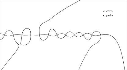
Figure 3. xray of $g(s)$ details

Notation: In this section, we will consider the values of $\mathop{\mathcal{R}}\nolimits(s)$ at the points $s=\sigma+it$ with $\sigma\leq 10$ and $t\geq 0$. For such values of $s$, we consider $\eta=\sqrt{\frac{s-1}{2\pi i}}$, selecting the root $\eta=\eta_{1}+i\eta_{2}$ with $\eta_{1}+\eta_{2}\geq 0$. When $\sigma\leq 1$ this means $0\leq\eta_{2}\leq\eta_{1}$. In this case $|e^{2\pi i\eta}|\leq 1$, with strict inequality for $\sigma<1$.

We want a value of $\sigma$ such that all zeros of $\mathop{\mathcal{R}}\nolimits(s)$ to height $T$ satisfies $\sigma\leq\mathop{\mathrm{Re}}\nolimits(\rho)$. This is obtained by means of the next Theorem proved in [7]*Th. 9.

Theorem 18.

There exist constants $A$ and $t_{0}>1$ such that for $s$ in the closed set

$$\Omega=\{s\in\mathbf{C}\colon t\geq t_{0},\quad 1-\sigma\geq t^{3/7}\},$$

we have

(16) $$\mathop{\mathcal{R}}\nolimits(s)=-\chi(s)\eta^{s-1}e^{-\pi i\eta^{2}}\frac{\sqrt{2}e^{3\pi i/8}\sin\pi\eta}{2\cos 2\pi\eta}(1+U(s)),\qquad|U(s)|\leq At^{-\frac{1}{21}},$$

where $\eta=\sqrt{(s-1)/2\pi i}$ satisfies $\mathop{\mathrm{Re}}\nolimits(\eta)+\mathop{\mathrm{Im}}\nolimits(\eta)>0$.

Lemma 19.

Let $t_{0}$ be a constant greater than the constant appearing in Theorem 18. For $s=\sigma+it$ with $t\geq t_{0}$ and $1-\sigma\geq t^{3/7}$, we have

$$F(s):=s\pi^{-s/2}\Gamma(s/2)\mathop{\mathcal{R}}\nolimits(s)=J(s)(1+U(s)),$$

where

(17) $$\log J(s)=\frac{\pi is}{4}+\log s-\frac{1}{2}\log\frac{1-s}{2\pi}-\frac{3\pi i}{8}+\pi i\eta+\log\frac{1-e^{2\pi i\eta}}{1+e^{4\pi i\eta}}+\mathop{\hbox{\cmbsy O}}\nolimits(|s|^{-1}).$$

Proof.

Since we assume that $s$ satisfies the conditions in Theorem 18 we have (16). Therefore, by definition, $F(s)=J(s)(1+U(s))$, where

$$J(s) =-s\pi^{-s/2}\Gamma(s/2)\chi(s)\eta^{s-1}e^{-\pi i\eta^{2}}\frac{\sqrt{2}e^{3\pi i/8}\sin\pi\eta}{2\cos 2\pi\eta}$$

$$=-s\pi^{(s-1)/2}\Gamma(\tfrac{1-s}{2})\eta^{s-1}e^{-\pi i\eta^{2}}\frac{\sqrt{2}e^{3\pi i/8}\sin\pi\eta}{2\cos 2\pi\eta}$$

$$=2^{-1/2}e^{-\pi i/8}s\pi^{(s-1)/2}\Gamma(\tfrac{1-s}{2})\eta^{s-1}e^{-\pi i\eta^{2}+\pi i\eta}\frac{1-e^{2\pi i\eta}}{1+e^{4\pi i\eta}}.$$

We may define a continuous logarithm of $J(s)$ for these values of $s$ by noticing that $|e^{2\pi i\eta}|<1$ and therefore we may use

$$\log\frac{1-e^{2\pi i\eta}}{1+e^{4\pi i\eta}}=-\sum_{n=1}^{\infty}\frac{z^{n}}{n}+\sum_{n=1}^{\infty}(-1)^{n}\frac{z^{2n}}{n},\qquad z=e^{2\pi i\eta}.$$

That is, it is equal to $\log(1-e^{2\pi i\eta})-\log(1+e^{4\pi i\eta})$, using in both cases the main branch of the logarithm. It follows that the imaginary part of $\log\frac{1-e^{2\pi i\eta}}{1+e^{4\pi i\eta}}$ is bounded by $\pi$. By the usual Euler-MacLaurin expansion, which is applicable since $\sigma<0$,

$$\log J(s)=-\frac{1}{2}\log 2-\frac{\pi i}{8}+\log s+\frac{s-1}{2}\log\pi-\frac{s}{2}\log\frac{1-s}{2}-\frac{1-s}{2}+\frac{1}{2}\log 2\pi\\ +\frac{s-1}{2}\log\frac{s-1}{2\pi i}-\pi i\frac{s-1}{2\pi i}+\pi i\eta+\log\frac{1-e^{2\pi i\eta}}{1+e^{4\pi i\eta}}+\mathop{\hbox{\cmbsy O}}\nolimits(|s|^{-1}).$$

Simplifying this yields

$$\log J(s)=\frac{\pi is}{4}+\log s-\frac{1}{2}\log(1-s)+\frac{1}{2}\log 2\pi-\frac{3\pi i}{8}+\pi i\eta+\log\frac{1-e^{2\pi i\eta}}{1+e^{4\pi i\eta}}+\mathop{\hbox{\cmbsy O}}\nolimits(|s|^{-1}).\qed$$

The next propositions will be proved later in Section 8.

Proposition 20.

Let $t_{0}>1$ and $0<a<\frac{1}{2}$ be fixed real numbers. There is a function $f\colon[0,+\infty)\to[0,+\infty)$ such that $f(T)=\mathop{\hbox{\cmmib o}}\nolimits(T^{1/2})$ and such that for $T>t_{0}$, $\sigma\leq 10$ and $1-\sigma\leq T^{a}$ we have

(18) $$\int_{t_{0}}^{T}\log|F(\sigma+it)|\,dt =-\frac{\pi T^{2}}{8}+(\sigma+1)\Bigl{(}\frac{T}{2}\log\frac{T}{2\pi}-\frac{T}{2}\Bigr{)}+\frac{T}{2}(\log 2+2\log(2\pi))$$

$$-\frac{\pi\sigma^{2}}{8}+\int_{t_{0}}^{T}\log|\mathop{\mathcal{R}}\nolimits(\sigma+it)|\,dt+\mathop{\hbox{\cmbsy O}}\nolimits(f(T)).$$

Proposition 21.

Let $1\leq t_{0}<T$ with $t_{0}$ bigger than the constant appearing in Theorem 18 and let $1-\sigma_{0}=T^{a}$ with $a=3/7$. Then we have

(19) $$\int_{t_{0}}^{T}\log|F(\sigma_{0}+it)|\,dt=-\frac{\pi T^{2}}{8}+\frac{T}{2}\log T-\frac{T}{2}+\frac{T}{2}\log 2\pi+\mathop{\hbox{\cmbsy O}}\nolimits(T^{20/21}).$$

Lemma 22.

Let $t_{0}$ and $\sigma_{0}$ be fixed real numbers satisfying $t_{0}>1$ and $\sigma_{0}<-1$. Assume that $F(s)$ does not vanish for $\mathop{\mathrm{Im}}\nolimits(s)=t_{0}$ and denote by $\arg F(\sigma+it_{0})$ a continuous determination of the argument, defined for $\sigma_{0}\leq\sigma\leq\sigma_{1}\leq 10$, and such that $|\arg F(\sigma_{0}+it_{0})|\leq C|\sigma_{0}|$. Then there is a constant $C_{0}$ (depending on $t_{0}$, and $C$ such that

$$\Bigl{|}\int_{\sigma_{0}}^{\sigma_{1}}\arg F(\sigma+it_{0})\,d\sigma\Bigr{|}\leq C_{0}|\sigma_{0}|^{2}\log|\sigma_{0}|.$$

Proof.

We have

$$|\arg F(\sigma+it_{0})-\arg F(\sigma_{0}+it_{0})|=\Bigl{|}\mathop{\mathrm{Re}}\nolimits\frac{1}{i}\int_{\sigma_{0}+it_{0}}^{\sigma+it_{0}}\frac{F^{\prime}(z)}{F(z)}\,dz\Bigr{|},$$

we may bound the integral by Backlund’s lemma. We take a disc $D$ with center at $10+it_{0}$ and radius $2(10-\sigma_{0})$. To bound $F$ on $D$, notice that $D$ is contained in a disc of center $0$ and radius $C|\sigma_{0}|$ (where the constant $C$ here depends only on $t_{0}$). In [10]*eq.(3) we have proved that $|F(s)|\leq Ae^{B|s|\log|s|}$. So that $|F(s)|\leq Ae^{c(t_{0})|\sigma_{0}|\log|\sigma_{0}|}$. Also, we have $|F(10+it_{0})|>0$ is a constant depending only on $t_{0}$. Therefore,

$$|\arg F(\sigma+it_{0})-\arg F(\sigma_{0}+it_{0})|\leq C|\sigma_{0}|\log|\sigma_{0}|.$$

It follows that $|F(\sigma+it_{0})|\leq C|\sigma_{0}|\log|\sigma_{0}|$. Then

$$\Bigl{|}\int_{\sigma_{0}}^{\sigma_{1}}\arg F(\sigma+it_{0})\,d\sigma\Bigr{|}\leq C|\sigma_{0}|^{2}\log|\sigma_{0}|.\qed$$

Lemma 23.

Let $0<a<\frac{1}{2}$ a fixed real number and for $T>1$ let $1-\sigma_{0}=T^{a}$ and $\sigma_{0}<\sigma_{1}\leq 10$. Then we have

$$\mathop{\mathrm{Im}}\nolimits\int_{\sigma_{0}+iT}^{\sigma_{1}+iT}\log(s\pi^{-s/2}\Gamma(s/2))\,ds=\mathop{\hbox{\cmbsy O}}\nolimits(T^{2a})$$

when we take a continuous branch of the logarithm where $\mathop{\mathrm{Im}}\nolimits\log(s\pi^{-s/2}\Gamma(s/2))$ at the point $s=s_{0}+iT$ is $\mathop{\hbox{\cmbsy O}}\nolimits(T^{a})$.

Proof.

By Euler-MacLaurin expansion we have

$$\mathop{\mathrm{Im}}\nolimits\log\Gamma((\sigma+iT)/2)=\frac{T}{2}\log\frac{T}{2}-\frac{T}{2}+\frac{\pi}{4}(\sigma-1)+\frac{2\sigma-\sigma^{2}}{4T}+\mathop{\hbox{\cmbsy O}}\nolimits(T^{-1}).$$

For $\sigma_{0}\leq\sigma\leq\sigma_{1}\leq 10$ we have $\sigma^{2}/T^{2}=\mathop{\hbox{\cmbsy O}}\nolimits(T^{-1})$ so that

$$\mathop{\mathrm{Im}}\nolimits\log(\sigma+iT)=\frac{\pi}{2}-\arctan\frac{\sigma}{T}=\frac{\pi}{2}-\frac{\sigma}{T}+\mathop{\hbox{\cmbsy O}}\nolimits(T^{-1})$$

After some simplifications, we obtain for $s=\sigma+iT$

$$\text{}\mathop{\mathrm{Im}}\nolimits\log(s\pi^{-s/2}\Gamma(s/2))=\frac{T}{2}\log\frac{T}{2\pi}-\frac{T}{2}-\frac{\sigma^{2}+2\sigma}{4T}+\frac{\pi}{4}+\frac{\pi\sigma}{4}+\mathop{\hbox{\cmbsy O}}\nolimits(T^{-1}).$$

After subtracting the multiple of $2\pi$ nearest to $\frac{T}{2}\log\frac{T}{2\pi}-\frac{T}{2}$, we get a branch of the logarithm equal to

$$\mathop{\mathrm{Im}}\nolimits\log(s\pi^{-s/2}\Gamma(s/2))=-\frac{\sigma^{2}+\sigma}{2T}+\frac{\pi}{4}+\frac{\pi\sigma}{4}+\mathop{\hbox{\cmbsy O}}\nolimits(1)=\frac{\pi\sigma}{4}+\mathop{\hbox{\cmbsy O}}\nolimits(1).$$

Therefore,

$$\Bigl{|}\mathop{\mathrm{Im}}\nolimits\int_{\sigma_{0}+iT}^{\sigma_{1}+iT}\log(s\pi^{-s/2}\Gamma(s/2))\,ds\Bigr{|}\leq\frac{\pi}{8}(\sigma_{1}^{2}-\sigma_{0}^{2})+C(\sigma_{1}-\sigma_{0})\leq CT^{2a}.\qed$$

Proof of Theorem 2.

For a given $T>t_{0}$ define $\sigma_{0}$ such that $1-\sigma_{0}=T^{a}$ with $a=3/7$. For $T\geq T_{0}$ we will have $\sigma_{0}<\sigma$. We apply Littlewood’s lemma in the rectangle $R=[\sigma_{0},\sigma]\times[t_{0},T]$ to the function $F(s)=s\pi^{-s/2}\Gamma(s/2)\mathop{\mathcal{R}}\nolimits(s)$. As we have seen in the proof of Theorem 1 we may assume that there is no zero of $F(s)$ on the lines $\mathop{\mathrm{Re}}\nolimits(s)=t_{0}$ and $\mathop{\mathrm{Re}}\nolimits(s)=T$. We take $t_{0}$ large enough so that Theorem 18 applies with $At_{0}^{-1/21}<1$. This implies that $F(s)$ do not vanish on the left-hand side of the rectangle $R$. Note that the zeros of $F(s)$ and $\mathop{\mathcal{R}}\nolimits(s)$ on $t>0$ are the same with the same multiplicities.

Here, it is in line $\mathop{\mathrm{Re}}\nolimits(s)=\sigma$ where we do not know the argument of $F(s)$. Hence we have

(20) $$\text{}\quad 2\pi\sum_{\begin{subarray}{c}\beta<\sigma\\ t_{0}<\gamma\leq T\end{subarray}}(\sigma-\beta)=\int_{t_{0}}^{T}\log|F(\sigma+it)|\,dt-\int_{t_{0}}^{T}\log|F(\sigma_{0}+it)|\,dt$$

$$+\int_{\sigma_{0}}^{\sigma}\arg F(x+it_{0})\,dx-\int_{\sigma_{0}}^{\sigma}\arg F(x+iT)\,dx,$$

where $\arg F(s)$ should be taken continuously in the broken line with vertices at $\sigma+it_{0}$, $\sigma_{0}+it_{0}$, $\sigma_{0}+iT$, $\sigma+iT$.

By Lemma 19 we have $\arg F(s)=\arg J(s)+\arg(1+U(s))$, with $s=\sigma_{0}+it$. By the election of $\sigma_{0}$, the function $\arg(1+U(\sigma_{0}+it))$ for $t_{0}\leq t\leq T$ is always between $-\pi/2$ and $\pi/2$. By (17) we easily see that $\arg F(\sigma+it)$ for $1-\sigma\geq t^{a}$, $t\geq t_{0}$ is equal to

$$\arg F(\sigma+it)=\frac{\pi\sigma}{4}+\frac{\pi}{2}-\arctan\frac{\sigma}{t}+\frac{1}{2}\Bigl{(}\frac{\pi}{2}-\arctan\frac{1-\sigma}{t}\Bigr{)}-\frac{3\pi}{8}\\ +\frac{\pi}{\sqrt{2\pi}}(t^{2}+(1-\sigma)^{2})^{1/4}\cos(\tfrac{1}{2}\arctan\tfrac{1-\sigma}{t})+\mathop{\hbox{\cmbsy O}}\nolimits(1).$$

Since $1-\sigma_{0}=T^{a}$ it follows that $\arg F(\sigma_{0}+it)$ varies continuously between the extreme values

$$\arg F(\sigma_{0}+iT)=\pi\sqrt{\frac{T}{2\pi}}+\mathop{\hbox{\cmbsy O}}\nolimits(T^{a})\qquad\arg F(\sigma_{0}+it_{0})=\frac{\pi\sigma_{0}}{4}+\mathop{\hbox{\cmbsy O}}\nolimits(T^{a/2}).$$

Therefore, $\arg F(\sigma_{0}+it_{0})=\mathop{\hbox{\cmbsy O}}\nolimits(T^{a})$ and the lemma 22 apply to show that

(21) $$\int_{\sigma_{0}}^{\sigma}\arg F(x+it_{0})\,dx=\mathop{\hbox{\cmbsy O}}\nolimits(T^{2a}\log T).$$

On the upper side for $s=x+iT$ with $\sigma_{0}\leq x\leq\sigma$ we have

$$\arg F(s)=\arg(s\pi^{-s/2}\Gamma(s/2))+\arg\mathop{\mathcal{R}}\nolimits(s)$$

where the arguments on the right-hand side should be taken continuous and such that at the point $s_{0}=\sigma_{0}+iT$ we have

$$\arg(s_{0}\pi^{-s_{0}/2}\Gamma(s_{0}/2))+\arg\mathop{\mathcal{R}}\nolimits(s_{0})=\arg F(s_{0})=\pi\sqrt{T/2\pi}+\mathop{\hbox{\cmbsy O}}\nolimits(T^{a}).$$

We have some freedom here; we may pick $\arg(s_{0}\pi^{-s_{0}/2}\Gamma(s_{0}/2))=\mathop{\hbox{\cmbsy O}}\nolimits(T^{a})$ so that Lemma 23 applies, and

(22) $$\int_{\sigma_{0}+iT}^{\sigma+iT}\arg(s\pi^{-s/2}\Gamma(s/2))\,ds=\mathop{\hbox{\cmbsy O}}\nolimits(T^{2a}).$$

Then we must take $\arg\mathop{\mathcal{R}}\nolimits(s_{0})=\mathop{\hbox{\cmbsy O}}\nolimits(T^{1/2})$. We apply the Backlund lemma to bound the integral of $\arg\mathop{\mathcal{R}}\nolimits(x+iT)$. We have

$$|\arg\mathop{\mathcal{R}}\nolimits(x+iT)-\arg\mathop{\mathcal{R}}\nolimits(\sigma_{0}+iT)|=\Bigl{|}\mathop{\mathrm{Re}}\nolimits\frac{1}{i}\int_{\sigma_{0}+iT}^{x+iT}\frac{\mathop{\mathcal{R}}\nolimits^{\prime}(z)}{\mathop{\mathcal{R}}\nolimits(z)}\,dz\Bigr{|}$$

To determine the value of $\arg\mathop{\mathcal{R}}\nolimits(x+iT)$, we apply Backlund’s lemma. Take a disc with center at $10+iT$ and radius $R=2(10-\sigma_{0})$. On this disc $|\mathop{\mathcal{R}}\nolimits(s)|$ is bounded, according to Proposition 12 and 13 in [3] by

$$\leq C\max(T^{1/2},T^{cT^{a}}).$$

The value in the center of the disc $|\mathop{\mathcal{R}}\nolimits(10+iT)|\geq 1/2$ by by Proposition 6 in [6]. Hence, we get

$$|\arg\mathop{\mathcal{R}}\nolimits(x+iT)-\arg\mathop{\mathcal{R}}\nolimits(\sigma_{0}+iT)|\leq CT^{a}\log T.$$

It follows that

$$|\arg\mathop{\mathcal{R}}\nolimits(x+iT)|\leq CT^{a}\log T+CT^{1/2}\leq CT^{1/2}.$$

From which we obtain

(23) $$\int_{\sigma_{0}+iT}^{\sigma+iT}\arg\mathop{\mathcal{R}}\nolimits(s)\,ds=CT^{1/2+a}.$$

Putting the results of Propositions 20, 21 and equations (21), (22) and (23) into equation (20) yields

$$2\pi\sum_{\begin{subarray}{c}\beta\leq\sigma\\ t_{0}<\gamma\leq T\end{subarray}}(\sigma-\beta) =-\frac{\pi T^{2}}{8}+(\sigma+1)\Bigl{(}\frac{T}{2}\log\frac{T}{2\pi}-\frac{T}{2}\Bigr{)}+\frac{T}{2}(\log 2+2\log(2\pi))-\frac{\pi\sigma^{2}}{8}$$

$$+\int_{t_{0}}^{T}\log|\mathop{\mathcal{R}}\nolimits(\sigma+it)|\,dt+\mathop{\hbox{\cmmib o}}\nolimits(T^{1/2})+\frac{\pi T^{2}}{8}-\frac{T}{2}\log T+\frac{T}{2}-\frac{T}{2}\log 2\pi$$

$$+\mathop{\hbox{\cmbsy O}}\nolimits(T^{20/21})+\mathop{\hbox{\cmbsy O}}\nolimits(T^{2a}\log T)+\mathop{\hbox{\cmbsy O}}\nolimits(T^{\frac{1}{2}+a}),$$

Since $a=3/7$ the largest error term is $\mathop{\hbox{\cmbsy O}}\nolimits(T^{20/21})$. The term with $\sigma^{2}$ is less than this error term. Simplifying yields (2). ∎

Remark 24.

We can not apply Backlund’s lemma in order to bound the integral of $\arg g(x+it_{0})$ in Siegel’s exposition [17]. To use $g(s)$ we also have the extra difficulty that the Euler-MacLaurin approximation to the gamma function is not valid near the negative real axis. This is the main reason to use our $F(s)$ function instead of the $g(s)$ function of Siegel.

8. Proof of Propositions 20 and 21

8.1. Mean value of $\log|\Gamma(s)|$

We denote by $B_{n}(x)$ the Bernoulli polynomial and by $\widetilde{B_{n}}(x)$ the periodic function with period $1$ and such that $\widetilde{B_{n}}(x)=B_{n}(x)$ for $0<x<1$. They satisfy $B_{n}(x)=(-1)^{n}B_{n}(1-x)$. For an odd index greater than $1$ we have $B_{2n+1}(0)=B_{2n+1}(1/2)=B_{2n+1}(1)=0$, and these are the only zeros of $B_{2n+1}(x)$ on the interval $[0,1]$.

Lemma 25.

Let $f\colon(a,b)\to[0,+\infty)$ be a positive and monotonous function, then

$$\Bigl{|}\int_{a}^{b}f(x)\widetilde{B_{3}}(x)\,dx\Bigr{|}\leq\frac{3}{64}\max(f(a),f(b)).$$

Proof.

Assume that $f$ is not increasing, the proof in the other case is similar. We have $B_{3}(x)=x(x-\frac{1}{2})(x-1)$, so $B_{3}(x)$ is positive in $(0,1/2)$ and negative in $(1/2,1)$. Define

$$a_{n}=\left|\int_{n/2}^{(n+1)/2}f(x)\widetilde{B_{3}}(x)\,dx\right|=(-1)^{n}\int_{n/2}^{(n+1)/2}f(x)\widetilde{B_{3}}(x)\,dx.$$

For any integer $k$, since $f(x+k)\geq f(1-x+k)$ for $0<x<\frac{1}{2}$

$$a_{2k}=\int_{k}^{k+1/2}f(x)\widetilde{B_{3}}(x)\,dx=\int_{0}^{1/2}f(x+k)\widetilde{B_{3}}(x)\,dx\geq\int_{0}^{1/2}f(1-x+k)x(x-\tfrac{1}{2})(x-1)\,dx$$

changing variables $y=1-x$

$$=\int_{1/2}^{1}f(y+k)(1-y)(\tfrac{1}{2}-y)(-y)\,dy=-\int_{1/2}^{1}f(y+k)\widetilde{B_{3}}(y)\,dy=\\ -\int_{k+1/2}^{k+1}f(y)\widetilde{B_{3}}(y)\,dy=a_{2k+1}.$$

In the same way, we prove $a_{2k+1}\geq a_{2k+2}$.

Suppose first that there exist $n<m$ such that

$$(n-1)/2<a\leq n/2\leq m/2\leq b<(m+1)/2.$$

If $n<m$ we will have

$$\int_{a}^{b}=\int_{a}^{n/2}+\int_{n/2}^{m/2}+\int_{m/2}^{b}=\int_{a}^{n/2}+\sum_{n\leq k<m}(-1)^{k}a_{k}+\int_{m/2}^{b},$$

the omitted integrand being $f(x)\widetilde{B_{3}}(x)$, and with $a_{n}\geq a_{n+1}\geq\cdots\geq a_{m}\geq 0$. Therefore, we have

$$\Bigl{|}\sum_{n\leq k<m}(-1)^{k}a_{k}\Bigr{|}=a_{n}-a_{n+1}+a_{n+2}-\cdots\pm a_{m-1}\leq a_{n}.$$

Therefore,

$$\Bigl{|}\int_{a}^{b}\Bigr{|}\leq\Bigl{|}\int_{a}^{n/2}\Bigr{|}+a_{n}+\Bigl{|}\int_{m/2}^{b}\Bigr{|}\leq 3\int_{(n-1)/2}^{n/2}f(a)|\widetilde{B_{3}}(x)|\,dx=\frac{3f(a)}{64}.$$

When $n=m$ or there is no fraction $n/2$ between $a$ and $b$, the inequality is easier to prove. If we assume that $f$ is increasing, we must substitute $f(a)$ by $f(b)$. So, in general, the inequality is true with the maximum between $f(a)$ and $f(b)$. ∎

With the same procedure, we may prove this Proposition.

Proposition 26.

Let $f\colon(a,b)\to[0,+\infty)$ be a positive and monotonous function, then for all $n\geq 0$

$$\Bigl{|}\int_{a}^{b}f(x)\widetilde{B_{2n+1}}(x)\,dx\Bigr{|}\leq(-1)^{n}3\Bigl{(}1-\frac{1}{2^{2n+2}}\Bigr{)}\frac{B_{2n+2}}{n+1}\max(f(a),f(b)).$$

Proposition 27.

For $\sigma\in\mathbf{R}$ and $T>1$ we have

(24) $$\int_{1}^{T}\log|\Gamma(\tfrac{\sigma+it}{2})|\,dt=\mathop{\mathrm{Im}}\nolimits\int_{\sigma+i}^{\sigma+iT}\bigl{(}(\tfrac{s-1}{2})\log\tfrac{s}{2}-\tfrac{s}{2}+\tfrac{1}{2}\log 2\pi+\tfrac{1}{6s}\bigr{)}\,ds+\mathop{\hbox{\cmbsy O}}\nolimits^{*}\Bigl{(}\frac{3\sqrt{3}}{16}\Bigr{)}.$$

Proof.

Since $\sigma$ and $T>0$ are arbitrary, we cannot directly use the Euler-MacLaurin expansion. Instead, we use an intermediate expression obtained in the course of the proof of the Euler-MacLaurin expansion [12]*p. 109. We have

$$\log\Gamma(s)=(s-\tfrac{1}{2})\log s-s+\tfrac{1}{2}\log 2\pi+\frac{B_{2}}{2s}-\int_{0}^{\infty}\frac{\widetilde{B}_{3}(x)\,dx}{3(s+x)^{3}},\qquad s+|s|\neq 0.$$

Since

$$\int_{1}^{T}\log|\Gamma(\tfrac{\sigma+it}{2})|\,dt=\mathop{\mathrm{Im}}\nolimits\int_{\sigma+i}^{\sigma+iT}\log\Gamma(\tfrac{s}{2})\,ds,$$

we proceed to bound

$$R:=\mathop{\mathrm{Im}}\nolimits\int_{\sigma+i}^{\sigma+iT}\int_{0}^{\infty}\frac{\widetilde{B}_{3}(x)\,dx}{3(s/2+x)^{3}}\,ds.$$

The integral converge absolutely, so we may apply Fubini’s Theorem. And we have

$$R =\mathop{\mathrm{Im}}\nolimits\int_{0}^{\infty}\widetilde{B}_{3}(x)\Bigl{(}\int_{\sigma+i}^{\sigma+iT}\frac{ds}{3(s/2+x)^{3}}\Bigr{)}\,dx$$

$$=\mathop{\mathrm{Im}}\nolimits\frac{4}{3}\int_{0}^{\infty}\widetilde{B}_{3}(x)\Bigl{(}\frac{1}{(\sigma+i+2x)^{2}}-\frac{1}{(\sigma+iT+2x)^{2}}\Bigr{)}\,dx$$

$$=\frac{4}{3}\int_{0}^{\infty}\widetilde{B}_{3}(x)\Bigl{(}-\frac{2(\sigma+2x)}{((\sigma+2x)^{2}+1)^{2}}+\frac{2T(\sigma+2x)}{((\sigma+2x)^{2}+T^{2})^{2}}\Bigr{)}\,dx$$

Note that $\sigma\in\mathbf{R}$ may be negative. The function $\frac{2Ty}{(y^{2}+T^{2})^{2}}$ is negative and decreases in $(-\infty,-T/\sqrt{3})$, negative and increases in $(-T/\sqrt{3},0)$, positive and increasing in $(0,T/\sqrt{3})$ and decreasing and positive in $(T/\sqrt{3},+\infty)$ Its maximum value is achieved at $y=T/\sqrt{3}$ when it takes the value $\frac{3\sqrt{3}}{8T^{2}}$. At $-T/\sqrt{3}$ it has a minimum value of $-\frac{3\sqrt{3}}{8T^{2}}$. Hence, we may separate the integral into at most four integrals where Lemma 25 applies and

$$\Bigl{|}\frac{4}{3}\int_{0}^{\infty}\frac{2T(\sigma+2x)\widetilde{B}_{3}(x)}{((\sigma+2x)^{2}+T^{2})^{2}}\,dx\Bigr{|}\leq\frac{4}{3}\cdot 4\cdot\frac{3}{64}\cdot\frac{3\sqrt{3}}{8T^{2}}=\frac{3\sqrt{3}}{32T^{2}}.$$

This is also valid for $T=1$, so we get $|R|\leq\frac{3\sqrt{3}}{16}$.

Then

$$\int_{1}^{T}\log|\Gamma(\tfrac{\sigma+it}{2})|\,dt=\mathop{\mathrm{Im}}\nolimits\int_{\sigma+i}^{\sigma+iT}\bigl{(}(\tfrac{s-1}{2})\log\tfrac{s}{2}-\tfrac{s}{2}+\tfrac{1}{2}\log 2\pi+\tfrac{1}{6s}\bigr{)}\,ds+\mathop{\hbox{\cmbsy O}}\nolimits^{*}\Bigl{(}\frac{3\sqrt{3}}{16}\Bigr{)}.\qed$$

The same is true if we take the lower limit of the integrals equal to $t_{0}\geq 1$.

A computation of this integral gives us

(25) $$\int_{t_{0}}^{T} \log|\Gamma(\tfrac{\sigma+it}{2})|\,dt=\Bigl{(}-\frac{T^{2}}{4}+\frac{\sigma^{2}}{4}-\frac{\sigma}{2}+\frac{1}{6}\Bigr{)}\arg(\sigma+iT)\quad$$

$$+\Bigl{(}\frac{\sigma T}{4}-\frac{T}{4}\Bigr{)}\log(\sigma^{2}+T^{2})-\sigma\Bigl{(}\frac{3T}{4}+\frac{T\log 2}{2}\Bigr{)}+\frac{T}{2}+\frac{T}{2}\log 2+\frac{T}{2}\log 2\pi$$

$$+\Bigl{(}\frac{t_{0}^{2}}{4}-\frac{\sigma^{2}}{4}+\frac{\sigma}{2}-\frac{1}{6}\Bigr{)}\arg(\sigma+it_{0})+\Bigl{(}\frac{t_{0}}{4}-\frac{\sigma t_{0}}{4}\Bigr{)}\log(\sigma^{2}+t_{0}^{2})+$$

$$+\sigma\Bigl{(}\frac{3t_{0}}{4}+\frac{t_{0}\log 2}{2}\Bigr{)}-\frac{t_{0}}{2}-\frac{t_{0}}{2}\log 2-\frac{t_{0}}{2}\log 2\pi+\mathop{\hbox{\cmbsy O}}\nolimits^{*}(3\sqrt{3}/16)$$

where the argument always refers to the main argument, since $t_{0}$ and $T>0$ for us $0<\arg(\sigma+it)<\pi$.

Proposition 28.

Let $t_{0}\geq 1$ and $0<a<\frac{1}{2}$ be fixed real numbers. There is a positive function $f\colon[0,+\infty)\to[0,+\infty)$ such that $f(T)=\mathop{\hbox{\cmmib o}}\nolimits(T^{1/2})$ and such that given real numbers $\sigma\leq 10$ and $T>t_{0}$, connected by $1-\sigma\leq T^{a}$, then

(26) $$\int_{t_{0}}^{T}\log|\Gamma(\tfrac{\sigma+it}{2})|\,dt =-\frac{\pi T^{2}}{8}+(\sigma-1)\Bigl{(}\frac{T}{2}\log\frac{T}{2}-\frac{T}{2}\Bigr{)}+\frac{T}{2}\log(2\pi)-\frac{\pi\sigma^{2}}{8}$$

$$+\mathop{\hbox{\cmbsy O}}\nolimits(f(T)).$$

Proof.

The value of the integral is given in (25). Assume first that $-2t_{0}<\sigma\leq 10$. In this case, many terms in (25) are bounded by a constant only depending on $t_{0}$. Eliminating these terms, we get

$$\int_{t_{0}}^{T} \log|\Gamma(\tfrac{\sigma+it}{2})|\,dt=-\frac{T^{2}}{4}\arg(\sigma+iT)+\Bigl{(}\frac{\sigma T}{4}-\frac{T}{4}\Bigr{)}\log(\sigma^{2}+T^{2})$$

$$-\sigma\Bigl{(}\frac{3T}{4}+\frac{T\log 2}{2}\Bigr{)}+\frac{T}{2}+\frac{T}{2}\log 2+\frac{T}{2}\log 2\pi+\mathop{\hbox{\cmbsy O}}\nolimits(t_{0}^{2}\log(1+t_{0})).$$

We have $\arg(\sigma+iT)=\frac{\pi}{2}-\arctan\frac{\sigma}{T}$ and $\log(\sigma^{2}+T^{2})=2\log T+\log(1+\sigma^{2}/T^{2})=2\log T+\mathop{\hbox{\cmbsy O}}\nolimits(T^{-2})$. Expanding the $\arctan$, we get (with constants only depending on $t_{0}$)

$$\int_{t_{0}}^{T}\log|\Gamma(\tfrac{\sigma+it}{2})|\,dt =-\frac{\pi T^{2}}{8}+\frac{T^{2}}{4}\Bigl{(}\frac{\sigma}{T}+\mathop{\hbox{\cmbsy O}}\nolimits(T^{-3})\Bigr{)}+\Bigl{(}\frac{\sigma T}{4}-\frac{T}{4}\Bigr{)}(2\log T+\mathop{\hbox{\cmbsy O}}\nolimits(T^{-2}))$$

$$-\sigma\Bigl{(}\frac{3T}{4}+\frac{T\log 2}{2}\Bigr{)}+\frac{T}{2}+\frac{T}{2}\log 2+\frac{T}{2}\log 2\pi+\mathop{\hbox{\cmbsy O}}\nolimits(1).$$

This is (26) except for the term $-\sigma^{2}/8$, that in this case is contained in the error term.

In the other case, when $\sigma_{0}\leq\sigma\leq-2t_{0}$, eliminating terms that are $\mathop{\hbox{\cmmib o}}\nolimits(T^{a})$ we get

$$\int_{t_{0}}^{T} \log|\Gamma(\tfrac{\sigma+it}{2})|\,dt=\Bigl{(}-\frac{T^{2}}{4}+\frac{\sigma^{2}}{4}\Bigr{)}\arg(\sigma+iT)+\Bigl{(}\frac{\sigma T}{4}-\frac{T}{4}\Bigr{)}\log(\sigma^{2}+T^{2})$$

$$-\sigma\Bigl{(}\frac{3T}{4}+\frac{T\log 2}{2}\Bigr{)}+\frac{T}{2}+\frac{T}{2}\log 2+\frac{T}{2}\log 2\pi-\frac{\sigma^{2}}{4}\arg(\sigma+it_{0})+\mathop{\hbox{\cmmib o}}\nolimits(T^{1/2})$$

since $\sigma<0$ we have

$$\arg(\sigma+iT)=\frac{\pi}{2}-\arctan\frac{\sigma}{T},\quad\arg(\sigma+it_{0})=\pi+\arctan\frac{t_{0}}{\sigma},$$

$$\log(\sigma^{2}+T^{2})=2\log T+\log(1+\sigma^{2}/T^{2}),\quad\log(\sigma^{2}+t_{0}^{2})=2\log|\sigma|+\log(1+t_{0}^{2}/\sigma^{2}),$$

which we may expand in convergent power series since $\sigma/T$ and $t_{0}/\sigma$ are in absolute value $<1$. Removing terms less than $\mathop{\hbox{\cmmib o}}\nolimits(T^{1/2})$ yields (26). ∎

8.2. Proof of Proposition 20

Proof of Proposition 20.

By the definition of $F$ we have

$$\int_{t_{0}}^{T}\log|F(\sigma+it)|\,dt=\int_{t_{0}}^{T}\log|(\sigma+it)\pi^{-\sigma/2}|\,dt+\int_{t_{0}}^{T}\log|\Gamma(\tfrac{\sigma+it}{2})|\,dt+\int_{t_{0}}^{T}\log|\mathop{\mathcal{R}}\nolimits(\sigma+it)|\,dt$$

$$\int_{t_{0}}^{T}\log|(\sigma+it)\pi^{-\sigma/2}|\,dt =-\sigma\frac{T-t_{0}}{2}\log\pi+\frac{T}{2}\log(\sigma^{2}+T^{2})-T+\sigma\arctan\frac{T}{\sigma}$$

$$-\frac{t_{0}}{2}\log(\sigma^{2}+t_{0}^{2})+t_{0}-\sigma\arctan\frac{t_{0}}{\sigma}.$$

After some simplifications

$$\int_{t_{0}}^{T}\log|(\sigma+it)\pi^{-\sigma/2}|\,dt=T\log T-T-\sigma\frac{T}{2}\log\pi+\mathop{\hbox{\cmmib o}}\nolimits(T^{1/2}).$$

Combining this with (26) yields

$$\int_{t_{0}}^{T}\log|F(\sigma+it)|\,dt =-\frac{\pi T^{2}}{8}+(\sigma+1)\Bigl{(}\frac{T}{2}\log\frac{T}{2\pi}-\frac{T}{2}\Bigr{)}+\frac{T}{2}(\log 2+2\log(2\pi))-\frac{\pi\sigma^{2}}{8}$$

$$+\int_{t_{0}}^{T}\log|\mathop{\mathcal{R}}\nolimits(\sigma+it)|\,dt+\mathop{\hbox{\cmmib o}}\nolimits(T^{1/2}).\qed$$

8.3. Proof of Proposition 21

Here we will assume that the exponent $a=3/7$. The error term we will obtain is determined by the error in Theorem 18 for $U(t)\ll t^{-1/21}$. This is not the best exponent, and its relation to $a=3/7$ is not as direct, as seen in [7]. Therefore, we will not be able to obtain in Proposition 21 an error better than $\mathop{\hbox{\cmbsy O}}\nolimits(T^{20/21})$. We suspect that Proposition 21 can be improved. Therefore, we will retain in our equations some terms less than the final error $\mathop{\hbox{\cmbsy O}}\nolimits(T^{20/21})$, always assuming that $a\leq 3/7$. In this way, we will get a conjecture about further terms in Proposition 6.

Definition 29.

We define a periodic function $\operatorname*{P}\colon\mathbf{R}\to\mathbf{R}$ by

(27) $$\operatorname*{P}(x)=\sum_{n=1}^{\infty}\frac{2\sin(2\pi nx)}{n^{2}}-\sum_{n=1}^{\infty}(-1)^{n}\frac{\sin(4\pi nx)}{n^{2}}.$$

Recall that for a given $s$ we define $\eta=\sqrt{(s-1)/2\pi i}$, taking the root such that $\mathop{\mathrm{Re}}\nolimits\eta+\mathop{\mathrm{Im}}\nolimits\eta>0$.

Lemma 30.

Let $t_{0}>1$ be a fixed real number. For $T\to+\infty$ we have

(28) $$\mathop{\mathrm{Im}}\nolimits\int_{1+it_{0}}^{1+iT}\log\frac{1-e^{2\pi i\eta}}{1+e^{4\pi i\eta}}\,ds=-\sqrt{T/2\pi}\;\operatorname*{P}(\sqrt{T/2\pi})+\mathop{\hbox{\cmbsy O}}\nolimits(1),$$

where the implicit constant only depends on $t_{0}$.

Proof.

Here $s=1+it$ with $t_{0}<t<T$ and $\eta=\sqrt{t/2\pi}$, hence

$$J:=\mathop{\mathrm{Im}}\nolimits\int_{1+it_{0}}^{1+iT}\log\frac{1-e^{2\pi i\eta}}{1+e^{4\pi i\eta}}\,ds=\mathop{\mathrm{Im}}\nolimits i\int_{t_{0}}^{T}\log\frac{1-e^{2\pi i\eta}}{1+e^{4\pi i\eta}}\,dt=\mathop{\mathrm{Re}}\nolimits\int_{t_{0}}^{T}\log\frac{1-e^{2\pi i\eta}}{1+e^{4\pi i\eta}}\,dt$$

Change variables $t=2\pi\eta^{2}$, and let $\tau_{0}=\sqrt{t_{0}/2\pi}$ and $\tau=\sqrt{T/2\pi}$, then

$$J=\mathop{\mathrm{Re}}\nolimits 4\pi\int_{\tau_{0}}^{\tau}\eta\log\frac{1-e^{2\pi i\eta}}{1+e^{4\pi i\eta}}\,d\eta$$

Now we use the expansion

(29) $$\log\frac{1-z}{1+z^{2}}=-\sum_{n=1}^{\infty}\frac{z^{n}}{n}+\sum_{n=1}^{\infty}(-1)^{n}\frac{z^{2n}}{n}.$$

Then we have (it is not difficult to justify the integration term by term)

$$J =4\pi\mathop{\mathrm{Re}}\nolimits\Bigl{\{}-\sum_{n=1}^{\infty}\frac{1}{n}\int_{\tau_{0}}^{\tau}\eta e^{2\pi in\eta}\,d\eta+\sum_{n=1}^{\infty}\frac{(-1)^{n}}{n}\int_{\tau_{0}}^{\tau}\eta e^{4\pi in\eta}\,d\eta\Bigr{\}}$$

$$=4\pi\mathop{\mathrm{Re}}\nolimits\Bigl{\{}\Bigl{.}\sum_{n=1}^{\infty}\Bigl{(}-\frac{e^{2\pi in\eta}}{4\pi^{2}n^{3}}+\frac{i\eta e^{2\pi in\eta}}{2\pi n^{2}}+(-1)^{n}\frac{e^{4\pi in\eta}}{16\pi^{2}n^{3}}-(-1)^{n}\frac{i\eta e^{4\pi in\eta}}{4\pi n^{2}}\Bigr{)}\Bigr{|}_{\tau_{0}}^{\tau}\Bigr{\}}$$

All terms in $\tau_{0}$ will contribute only to a term $\mathop{\hbox{\cmbsy O}}\nolimits(1)$ (with a constant dependent on $t_{0}$). Analogously, the term in $\tau$ and $n^{3}$, which do not have the factor $\eta$ also contributes to a term $\mathop{\hbox{\cmbsy O}}\nolimits(1)$ (this time with absolute constants). So, we get

$$J=\mathop{\mathrm{Re}}\nolimits\sum_{n=1}^{\infty}\Bigl{(}\frac{2i\tau e^{2\pi in\tau}}{n^{2}}-(-1)^{n}\frac{i\tau e^{4\pi in\tau}}{n^{2}}\Bigr{)}+\mathop{\hbox{\cmbsy O}}\nolimits(1)=\mathop{\mathrm{Re}}\nolimits i\tau\sum_{n=1}^{\infty}\Bigl{(}\frac{2e^{2\pi in\tau}}{n^{2}}-(-1)^{n}\frac{e^{4\pi in\tau}}{n^{2}}\Bigr{)}+\mathop{\hbox{\cmbsy O}}\nolimits(1)$$

$$=\tau\sum_{n=1}^{\infty}\Bigl{(}-\frac{2\sin(2\pi n\tau)}{n^{2}}+(-1)^{n}\frac{\sin(4\pi n\tau)}{n^{2}}\Bigr{)}+\mathop{\hbox{\cmbsy O}}\nolimits(1)=-\tau\operatorname*{P}(\tau)+\mathop{\hbox{\cmbsy O}}\nolimits(1).\qed$$

The previous lemma considers the integral with limits $1+it_{0}$ and $1+iT$, but we are interested in this integral with limits $\sigma_{0}+it_{0}$ and $\sigma_{0}+iT$. The difference between the two is bounded in the next lemma.

Lemma 31.

Let $0<a\leq 3/7$ and $1-\sigma\leq T^{a}$, then for $T\to+\infty$ we have

(30) $$\mathop{\mathrm{Im}}\nolimits\int_{\sigma+it_{0}}^{1+it_{0}}\log\frac{1-e^{2\pi i\eta}}{1+e^{4\pi i\eta}}\,ds-\mathop{\mathrm{Im}}\nolimits\int_{\sigma+iT}^{1+iT}\log\frac{1-e^{2\pi i\eta}}{1+e^{4\pi i\eta}}\,ds=\mathop{\hbox{\cmbsy O}}\nolimits(T^{a}).$$

Proof.

The two integrals are treated in the same way. For the second, for example, we have $s=x+iT$, with $\sigma<x<1$. Then as we noticed before $|e^{2\pi i\eta}|<1$ and the logarithm is defined by means of (29) with $z=e^{2\pi i\eta}$. Both series in (29) have imaginary parts in $(-\pi/2,\pi/2)$ so that

$$\Bigl{|}\mathop{\mathrm{Im}}\nolimits\int_{\sigma+iT}^{1+iT}\log\frac{1-e^{2\pi i\eta}}{1+e^{4\pi i\eta}}\,ds\Bigr{|}=\Bigl{|}\int_{\sigma}^{1}\mathop{\mathrm{Im}}\nolimits\log\frac{1-e^{2\pi i\eta}}{1+e^{4\pi i\eta}}\,dx\Bigr{|}\leq\int_{\sigma}^{1}\pi\,dx=\pi(1-\sigma)=\mathop{\hbox{\cmbsy O}}\nolimits(T^{a}).\qed$$

Lemma 32.

Let $1\leq t_{0}$ and $a\leq\frac{3}{7}$ be fixed real numbers and $1-\sigma_{0}=T^{a}$.

Then for $T\to+\infty$ we have

(31) $$\int_{t_{0}}^{T}\log|e^{\pi i\eta}|\,dt=-\pi(1-\sigma_{0})\Bigl{(}\frac{T}{2\pi}\Bigr{)}^{1/2}+\frac{\sqrt{\pi}}{3}(1-\sigma_{0})^{3/2}+\mathop{\hbox{\cmbsy O}}\nolimits(T^{a/2}).$$

Proof.

Put $s=\sigma_{0}+it$, then

$$\int_{t_{0}}^{T}\log|e^{\pi i\eta}|\,dt=\mathop{\mathrm{Im}}\nolimits\int_{\sigma+it_{0}}^{\sigma+iT}\log e^{\pi i\eta}\,ds=\mathop{\mathrm{Im}}\nolimits\int_{\sigma+it_{0}}^{\sigma+iT}\pi i\sqrt{\frac{s-1}{2\pi i}}\,ds$$

$$=-\mathop{\mathrm{Im}}\nolimits\int_{\sigma+it_{0}}^{\sigma+iT}2\pi^{2}\sqrt{\frac{s-1}{2\pi i}}\,d\frac{s-1}{2\pi i}=-2\pi^{2}\mathop{\mathrm{Im}}\nolimits\Bigl{.}\frac{1}{3/2}\Bigl{(}\frac{s-1}{2\pi i}\Bigr{)}^{3/2}\Bigr{|}_{s=\sigma+it_{0}}^{\sigma+iT}$$

$$=-\frac{4\pi^{2}}{3}\mathop{\mathrm{Im}}\nolimits\Bigl{\{}\Bigl{(}\frac{T}{2\pi}+i\frac{1-\sigma}{2\pi}\Bigr{)}^{3/2}-\Bigl{(}\frac{t_{0}}{2\pi}+i\frac{1-\sigma}{2\pi}\Bigr{)}^{3/2}\Bigr{\}}$$

$$=\mathop{\mathrm{Im}}\nolimits\Bigl{\{}-\frac{4\pi^{2}}{3}\Bigl{(}\frac{T}{2\pi}\Bigr{)}^{3/2}\Bigl{(}1+i\frac{1-\sigma}{T}\Bigr{)}^{3/2}+\frac{4\pi^{2}}{3}\Bigl{(}i\frac{1-\sigma}{2\pi}\Bigr{)}^{3/2}\Bigl{(}1-i\frac{t_{0}}{1-\sigma}\Bigr{)}^{3/2}\Bigr{\}}.$$

According to the hypothesis, both $(1-\sigma)/T$ and $t_{0}/(1-\sigma)$ are less than $\frac{1}{2}$, say. So, we may expand both parenthesis in convergent power series. If I want to get this with an error $\mathop{\hbox{\cmmib o}}\nolimits(1)$ we must retain the terms until $((1-\sigma)/T)^{3}$ and $(t_{0}/(1-\sigma))^{2}$. Therefore, the result is the imaginary part of

$$\mathop{\mathrm{Im}}\nolimits\Bigl{\{}-\frac{4\pi^{2}}{3}\Bigl{(}\frac{T}{2\pi}\Bigr{)}^{3/2}\Bigl{(}1+\frac{3i}{2}\frac{1-\sigma}{T}-\frac{3}{8}\frac{(1-\sigma)^{2}}{T^{2}}\Bigr{)}+\mathop{\hbox{\cmbsy O}}\nolimits((1-\sigma)^{3}T^{-3/2})$$

$$+(-1+i)\frac{4\pi^{2}}{3\sqrt{2}}\Bigl{(}\frac{1-\sigma}{2\pi}\Bigr{)}^{3/2}\Bigl{(}1-\frac{3i}{2}\frac{t_{0}}{1-\sigma}\Bigr{)}+\mathop{\hbox{\cmbsy O}}\nolimits((1-\sigma)^{-1/2})\Bigr{\}}$$

$$\int_{t_{0}}^{T}\log|e^{\pi i\eta}|\,dt=-\frac{4\pi^{2}}{3}\Bigl{(}\frac{T}{2\pi}\Bigr{)}^{3/2}\frac{3}{2}\frac{1-\sigma}{T}+\frac{4\pi^{2}}{3\sqrt{2}}\Bigl{(}\frac{1-\sigma}{2\pi}\Bigr{)}^{3/2}\\ +\frac{4\pi^{2}}{3\sqrt{2}}\frac{3}{2}\Bigl{(}\frac{1-\sigma}{2\pi}\Bigr{)}^{3/2}\frac{t_{0}}{1-\sigma}+\mathop{\hbox{\cmbsy O}}\nolimits((1-\sigma)^{3}T^{-3/2})+\mathop{\hbox{\cmbsy O}}\nolimits((1-\sigma)^{-1/2})$$

$$=-\pi(1-\sigma)\Bigl{(}\frac{T}{2\pi}\Bigr{)}^{1/2}+\frac{\sqrt{\pi}}{3}(1-\sigma)^{3/2}+\frac{t_{0}}{2}(\pi(1-\sigma))^{1/2}+\mathop{\hbox{\cmbsy O}}\nolimits((1-\sigma)^{-1/2})$$

assuming that $a\leq\frac{3}{7}$ so that the exponent $3a-3/2\leq-a/2$ . ∎

Proposition 33.

Let $t_{0}>1$ greater than the constant in Theorem 18 and $1-\sigma_{0}=T^{a}$ with $0<a<1/2$. Then, for $T\to+\infty$

(32) $$\int_{t_{0}}^{T}\log|J(\sigma_{0}+it)|\,dt=-\frac{\pi T^{2}}{8}+\frac{T}{2}\log T-\frac{T}{2}+\frac{T}{2}\log(2\pi)+\mathop{\hbox{\cmbsy O}}\nolimits(T^{a+\frac{1}{2}})$$

Proof.

By Lemmas 19, 30, 31 and 32, it remains to compute

$$A=\mathop{\mathrm{Im}}\nolimits\int_{\sigma_{0}+it_{0}}^{\sigma_{0}+iT}\Bigl{(}\frac{\pi is}{4}+\log s-\frac{1}{2}\log\frac{1-s}{2\pi}-\frac{3\pi i}{8}\Bigr{)}\,ds$$

$$A=\mathop{\mathrm{Im}}\nolimits\Bigl{\{}\Bigl{.}\frac{\pi is^{2}}{8}+s\log s-\frac{1}{2}s-\frac{3\pi is}{8}+\frac{1-s}{2}\log\frac{1-s}{2\pi}\Bigr{|}_{\sigma_{0}+it_{0}}^{\sigma_{0}+iT}\Bigr{\}}$$

$$=-\frac{\pi T^{2}}{8}-\frac{T}{2}+\mathop{\hbox{\cmbsy O}}\nolimits_{t_{0}}(1)+\mathop{\mathrm{Im}}\nolimits\Bigl{\{}(\sigma_{0}+iT)\log(\sigma_{0}+iT)-(\sigma_{0}+it_{0})\log(\sigma_{0}+it_{0})\\ +\frac{1-\sigma_{0}-iT}{2}\log\frac{1-\sigma_{0}-iT}{2\pi}-\frac{1-\sigma_{0}-it_{0}}{2}\log\frac{1-\sigma_{0}-it_{0}}{2\pi}\Bigr{\}}$$

Simple computations yields (I have written here $\sigma$ instead of $\sigma_{0}$)

$$\text{}\quad\mathop{\mathrm{Im}}\nolimits(\sigma+iT)\log(\sigma+iT)=T\log T-T\sum_{n=1}^{\infty}\frac{(-1)^{n}}{2n}\Bigl{(}\frac{\sigma}{T}\Bigr{)}^{2n}+\frac{\pi\sigma}{2}+\sigma\sum_{n=1}^{\infty}\frac{(-1)^{n}}{2n-1}\Bigl{(}\frac{\sigma}{T}\Bigr{)}^{2n-1}.$$

$$\text{}\quad\mathop{\mathrm{Im}}\nolimits(\sigma+it_{0})\log(\sigma+it_{0})=t_{0}\log|\sigma|-t_{0}\sum_{n=1}^{\infty}\frac{(-1)^{n}}{2n}\Bigl{(}\frac{t_{0}}{\sigma}\Bigr{)}^{2n}+\pi\sigma-\sigma\sum_{n=1}^{\infty}\frac{(-1)^{n}}{2n-1}\Bigl{(}\frac{t_{0}}{\sigma}\Bigr{)}^{2n-1}.$$

$$\text{}\quad\mathop{\mathrm{Im}}\nolimits\Bigl{(}\frac{1-\sigma}{2}-\frac{iT}{2}\Bigr{)}\log\frac{1-\sigma-iT}{2\pi}\\ =-\frac{T}{2}\log\frac{T}{2\pi}+\frac{T}{2}\sum_{n=1}^{\infty}\frac{(-1)^{n}}{2n}\Bigl{(}\frac{1-\sigma}{T}\Bigr{)}^{2n}-\frac{\pi(1-\sigma)}{4}-\frac{1-\sigma}{2}\sum_{n=1}^{\infty}\frac{(-1)^{n}}{2n-1}\Bigl{(}\frac{1-\sigma}{T}\Bigr{)}^{2n-1}.$$

$$\hbox{}\quad\mathop{\mathrm{Im}}\nolimits\Bigl{(}\frac{1-\sigma}{2}-\frac{it_{0}}{2}\Bigr{)}\log\frac{1-\sigma-it_{0}}{2\pi}\\ =-\frac{t_{0}}{2}\log\frac{1-\sigma}{2\pi}+\frac{t_{0}}{2}\sum_{n=1}^{\infty}\frac{(-1)^{n}}{2n}\Bigl{(}\frac{t_{0}}{1-\sigma}\Bigr{)}^{2n}+\frac{1-\sigma}{2}\sum_{n=1}^{\infty}\frac{(-1)^{n}}{2n-1}\Bigl{(}\frac{t_{0}}{1-\sigma}\Bigr{)}^{2n-1}\Bigr{)}.$$

Substituting these values, we obtain

$$A=-\frac{\pi T^{2}}{8}-\frac{T}{2}+T\log T-\frac{T}{2}\log\frac{T}{2\pi}+\mathop{\hbox{\cmbsy O}}\nolimits(T^{a}).$$

$$A=-\frac{\pi T^{2}}{8}+\frac{T}{2}\log T-\frac{T}{2}+\frac{T}{2}\log 2\pi+\mathop{\hbox{\cmbsy O}}\nolimits(T^{a}).$$

By the above lemmas 19, 30, 31 and 32 we get then

$$\int_{t_{0}}^{T} \log|J(\sigma_{0}+it)|\,dt=-\frac{\pi T^{2}}{8}+\frac{T}{2}\log T-\frac{T}{2}+\frac{T}{2}\log 2\pi+\mathop{\hbox{\cmbsy O}}\nolimits(T^{a})$$

$$-\pi(1-\sigma_{0})\Bigl{(}\frac{T}{2\pi}\Bigr{)}^{1/2}+\frac{\sqrt{\pi}}{3}(1-\sigma_{0})^{3/2}+\mathop{\hbox{\cmbsy O}}\nolimits(T^{a/2})$$

$$-\Bigl{(}\frac{T}{2\pi}\Bigr{)}^{1/2}\operatorname*{P}(\sqrt{T/2\pi})+\mathop{\hbox{\cmbsy O}}\nolimits(1).$$

Therefore,

(33) $$\int_{t_{0}}^{T}\log|J(\sigma_{0}+it) |\,dt=-\frac{\pi T^{2}}{8}+\frac{T}{2}\log T-\frac{T}{2}+\frac{T}{2}\log 2\pi+\pi\sigma_{0}\Bigl{(}\frac{T}{2\pi}\Bigr{)}^{1/2}$$

$$-\bigl{(}\pi+\operatorname*{P}(\sqrt{T/2\pi})\bigr{)}\Bigl{(}\frac{T}{2\pi}\Bigr{)}^{1/2}+\frac{\sqrt{\pi}}{3}(1-\sigma_{0})^{3/2}+\mathop{\hbox{\cmbsy O}}\nolimits(T^{a}).$$

∎

Remark 34.

Siegel [17]*p. 304 asserts that he can prove his theorems with $a=\varepsilon$. This would imply that the term containing the function $P$ in equation (33) would make sense. In [2] we saw that this term appears in the experimental data obtained with the zeros of $\mathop{\mathcal{R}}\nolimits(s)$.

Proof of Proposition 21.

Since $t_{0}$ is chosen adequately, we have by Theorem 18 that $F(s)=J(s)(1+U(s))$, with $|U(s)|\leq At^{-1/21}$. It follows that

$$\int_{t_{0}}^{T}\log|1+U(\sigma_{0}+it)|\,dt=\mathop{\hbox{\cmbsy O}}\nolimits(T^{20/21}).$$

Combining this with Proposition 33 proves Proposition 21. ∎

References

- [1] J. Arias de Reyna, Riemann’s auxiliary function: Basic Results, arXiv:2406.02403.
- [2] J. Arias de Reyna, Statistics of zeros of the auxiliary function, arXiv:2406.03041.
- [3] J. Arias de Reyna, Simple bounds of the auxiliary function of Riemann, preprint (92).
- [4] J. Arias de Reyna, Region without zeros for the auxiliary function of Riemann, arXiv:2406.03825.
- [5] J. Arias de Reyna, Asymptotic expansions of the auxiliary function, arXiv:2406.04714.
- [6] J. Arias de Reyna, Riemann’s auxiliary function. Right Limit of zeros, arXiv:2406.07014.
- [7] J. Arias de Reyna, Note on the asymptotic of the auxiliary function, arXiv:2406.06066.
- [8] J. Arias de Reyna, Mean values of the auxiliary function, preprint (101).
- [9] J. Arias de Reyna, On the number of zeros of , preprint (185).
- [10] J. Arias de Reyna, Infinite product of Riemann auxiliary function, preprint (66).
- [11] R. J. Backlund, Sur les zéros de la fonction de Riemann, Comptes Rendues de l’Académie des Sciences 158 (1914) 1979–1981.
- [12] H. M. Edwards, Riemann’s Theta Function, Academic Press, 1974, [Dover Edition in 2001].
- [13] J. E. Littlewood, On the zeros of the Riemann zeta-function, Proc. Cambridge Philos. Soc. 22 (1924) 295–318, doi:10.1017/S0305004100014225
- [14] B. Riemann, Über die Anzahl der Primzahlen unter einer gegebenen Grösse, Monatsber. Akad. Berlin (1859) 671–680.
- [15] B. Riemann, Gesamemelte Mathematische Werke, Wissenschaftlicher Nachlass und Nachträge—Collected Papers, Ed. R. Narasimhan, Springer, 1990.
- [16] W. Rudin, Real and complex analysis, McGraw-Hill, London, 1970.
- [17] C. L. Siegel, Über Riemann Nachlaß zur analytischen Zahlentheorie, Quellen und Studien zur Geschichte der Mathematik Astronomie und Physik 2 (1932) 45–80. (Reprinted in [18], 1, 275–310.) English version.
- [18] C. L. Siegel, Carl Ludwig Siegel’s Gesammelte Abhandlungen, (edited by K. Chandrasekharan and H. Maaß), Springer-Verlag, Berlin, 1966.
- [19] E. C. Titchmarsh The Theory of the Riemann Zeta-function, Second edition. Edited and with a preface by D. R. Heath-Brown. The Clarendon Press, Oxford University Press, New York, 1986.