DPSW-Sketch: A Differentially Private Sketch Framework for Frequency Estimation over Sliding Windows (Technical Report)

Abstract.

The sliding window model of computation captures scenarios in which data are continually arriving in the form of a stream, and only the most recent $w$ items are used for analysis. In this setting, an algorithm needs to accurately track some desired statistics over the sliding window using a small space. When data streams contain sensitive information about individuals, the algorithm is also urgently needed to provide a provable guarantee of privacy. In this paper, we focus on the two fundamental problems of privately (1) estimating the frequency of an arbitrary item and (2) identifying the most frequent items (i.e., heavy hitters), in the sliding window model. We propose DPSW-Sketch, a sliding window framework based on the count-min sketch that not only satisfies differential privacy over the stream but also approximates the results for frequency and heavy-hitter queries within bounded errors in sublinear time and space w.r.t. $w$. Extensive experiments on five real-world and synthetic datasets show that DPSW-Sketch provides significantly better utility-privacy trade-offs than state-of-the-art methods.

1. Introduction

Many real-world applications, including Internet of Things (IoT), location-based services, and public health surveillance, generate large volumes of time-evolving data. These data are typically collected continuously in the form of streams. Therefore, the design and analysis of streaming algorithms (Muthukrishnan, 2005), which primarily aim to provide accurate estimations over the stream in real time using a small space, has attracted much attention in the literature.

As data streams often contain sensitive information about individuals, such as browsing history, GPS coordinates, and health status, releasing the estimates computed on them without adequate protection can cause harmful privacy leakage. To address this issue, differential privacy (Dwork et al., 2006b) (DP), the de facto standard for privacy preservation, has been widely adopted in streaming analytics (Dwork et al., 2010; Chan et al., 2011). Informally, a randomized algorithm provides (event-level) DP if the output distribution of the algorithm is approximately the same when executed on a stream and any of its neighbors that differ from it by one item. This condition prevents an attacker with access to the output from inferring the existence of any individual item.

Furthermore, in practice, it is often essential to restrict the computation to recent data. For example, Apple’s DP team claims to retain the collected data for a maximum of three months (Upadhyay, 2019), and Google’s privacy policy states that browser data can be stored for up to nine months (Google, 2024). Such recency requirements are captured by the sliding window model (Datar et al., 2002; Braverman and Ostrovsky, 2007), where only the latest $w$ items in the stream are used for computation. In such scenarios, an algorithm should maintain and release real-time statistics continuously over the sliding window with differential privacy. Especially, we focus on two fundamental data statistics with numerous applications, including anomaly detection (Zhong et al., 2021), change detection (Haug et al., 2022), and autocomplete suggestions (Zhu et al., 2020), namely, frequency, i.e., the number of occurrences of any given item, and heavy hitters, i.e., the set of items that appear at least a given number of times.

For frequency estimation and heavy-hitter detection problems, sketches, which are compact probabilistic data structures to summarize streams (Cormode et al., 2012), have been widely employed for their high accuracy and efficiency. However, despite several attempts to extend the sketches to work in the sliding window model while guaranteeing differential privacy (Chan et al., 2012; Upadhyay, 2019; Blocki et al., 2023), these approaches have two main limitations that make them incapable of meeting the need for real-time stream analysis. First, their theoretical analyses are specific to heavy hitters and cannot provide any error bound for frequency estimation on the remaining items. Second, even for heavy hitters, these methods still fail to obtain accurate query results within reasonable privacy budgets and sketch sizes in practice.

Our Contributions

In this work, we propose a novel sketch framework with event-level differential privacy, called DPSW-Sketch, for frequency estimation in the sliding window model. Specifically, DPSW-Sketch divides the stream into disjoint substreams of equal length. Within each substream, it creates a series of checkpoints according to the idea of smooth histograms (Braverman and Ostrovsky, 2007). Then, it constructs a Private Count-Min Sketch (Zhao et al., 2022) (PCMS) for each checkpoint, which corresponds to all items either from the beginning of the substream to the checkpoint or from the checkpoint to the end of the substream. As such, it does not need to store any item after the item is processed, and it can maintain each PCMS incrementally without handling implicit item deletion over the sliding window. Furthermore, we design an efficient scheme to allocate the privacy budget across different PCMSs in each substream such that DPSW-Sketch provides $(\varepsilon,\delta)$-differential privacy for any given $\varepsilon>0$ and $\delta\in(0,1)$ throughout the stream, owing to the reduction from zero-Concentrated Differential Privacy (zCDP) (Bun and Steinke, 2016) to DP and the adaptive composition of zCDP. For any frequency or heavy-hitter query on the sliding window $W_{t}$ at any time $t$, it selects one PCMS per substream so that the concatenation of their corresponding items is closest to $W_{t}$ and combines the item frequencies obtained from all selected PCMSs to compute the result. Our theoretical analysis shows that DPSW-Sketch can estimate the frequency of an arbitrary item in $W_{t}$ within a bounded additive error. This approximation can be naturally extended to the problem of heavy-hitter identification. Meanwhile, DPSW-Sketch has sublinear time and space complexities w.r.t. the window size $w$. Finally, extensive experimental findings on five real-world and synthetic datasets confirm the superior performance of DPSW-Sketch compared to several state-of-the-art differentially private sliding-window sketches for frequency and heavy-hitter queries. In summary, the main contributions of this paper include:

• We present the DPSW-Sketch framework and thoroughly analyze its approximation guarantees for frequency and heavy-hitter queries as well as time and space complexities. In particular, we indicate that DPSW-Sketch achieves improved theoretical results over existing methods (Chan et al., 2012; Upadhyay, 2019; Blocki et al., 2023) with lower error bounds and/or complexities.

• We demonstrate that DPSW-Sketch provides much more accurate results for frequency and heavy-hitter queries using a smaller space than the sketches proposed in (Chan et al., 2012; Upadhyay, 2019; Blocki et al., 2023) under the same privacy budget.

Reproducibility

Our code and data are publicly available at https://github.com/wypsz/DP-Sliding-Window.

2. Related Work

Sketching techniques (Cormode et al., 2012) have attracted long-standing attention in the literature. As for frequency estimation and heavy-hitter detection problems, classic sketching methods include Count-Min Sketch (CMS) (Cormode and Muthukrishnan, 2005), CountSketch (Charikar et al., 2004), CU sketch (Estan and Varghese, 2002), Misra-Gries (MG) sketch (Misra and Gries, 1982), etc. On the basis of these sketches, numerous non-private frameworks were proposed for frequency and heavy-hitter queries over sliding windows, e.g., (Arasu and Manku, 2004; Papapetrou et al., 2012; Rivetti et al., 2015; Ben-Basat et al., 2016; Gou et al., 2020; Wu et al., 2023). Unfortunately, the above frameworks do not provide any privacy guarantee and can potentially leak sensitive user data.

Differentially private sketches for frequency and heavy-hitter queries were proposed in (Mir et al., 2011; Melis et al., 2016; Yildirim et al., 2020; Huang et al., 2022; Zhao et al., 2022; Pagh and Thorup, 2022; Lebeda and Tetek, 2023; Fichtenberger et al., 2023; Andersson and Pagh, 2023). These sketches can provide provable guarantees of both privacy and accuracy while not reducing efficiency. However, they cannot handle implicit deletions of items and thus cannot work in the sliding window model. Among the existing literature, the works most related to ours are (Chan et al., 2012; Upadhyay, 2019; Blocki et al., 2023), which proposed sketching methods for heavy-hitter identification with event-level differential privacy in the sliding window model. Chan et al. (2012) first proposed a differentially private algorithm based on MG sketches for heavy-hitter identification in the (distributed) sliding window model. Upadhyay (2019) designed a sliding-window framework to privately identify heavy hitters and estimate their frequencies based on CountSketch and CMS. Blocki et al. (2023) proposed an improved method for private heavy-hitter queries by combining MG sketches with hierarchical counters. Compared to (Chan et al., 2012; Upadhyay, 2019; Blocki et al., 2023), our work achieves better theoretical results by (1) providing approximations for the frequencies of all items, instead of only those of heavy hitters, and (2) reducing the error bound for heavy hitters and complexity (see Section 4.2 for a detailed comparison). Our proposed method also demonstrates substantial improvements in practical performance compared to the methods proposed in (Chan et al., 2012; Upadhyay, 2019; Blocki et al., 2023), as will be shown in Section 5.

Differentially private sketches for other stream statistics, such as quantiles (Perrier et al., 2019; Gillenwater et al., 2021; Kaplan et al., 2022; Ben-Eliezer et al., 2022), moments (Wang et al., 2022; Epasto et al., 2023), and cardinality (Smith et al., 2020; Hehir et al., 2023; Ghazi et al., 2023), have also received significant attention. The sketches employed in the above problems differ from those in frequency estimation and thus are not comparable to our framework in this paper.

3. Preliminaries

For a positive integer $n$, we use $[n]$ to denote $[1,\dots,n]$. A data stream is an (ordered) sequence of $n$ items $S=[s_{1},s_{2},\dots,s_{n}]$, where $s_{i}$ is the $i$-th item and is drawn from a domain $\mathcal{E}$ of size $m$ indexed by $[m]$. Then, $S_{t}=[s_{1},\dots,s_{t}]$ denotes the prefix of $S$ until the arrival of $s_{t}$ at any time $t\leq n$. A count-based sliding window $W_{t}$ of length $w\in\mathbb{Z}^{+}$ at time $t$ is the union of the latest $w$ items in $S_{t}$, i.e., $W_{t}=\{s_{i}\in S_{t}:\max(t-w+1,1)\leq i\leq t\}$. Note that our framework can be applied to other types of sliding windows, e.g., time-based sliding windows that contain all the items in the last $w$ time units. For ease of presentation, we focus on count-based sliding windows in this work. We consider two fundamental statistics over sliding windows: frequency and heavy hitter. Specifically, the frequency $f_{e,t}$ of an item $e\in\mathcal{E}$ in $W_{t}$ is the number of occurrences of $e$ in $W_{t}$, i.e., $f_{e,t}=\left|\{s_{i}\in W_{t}:s_{i}=e\}\right|$. Items with high frequencies are often called heavy hitters. Given a threshold $\gamma\in(0,1)$, an item is a $\gamma$-heavy hitter in $W_{t}$ if its frequency in $W_{t}$ is at least $\gamma w$. Formally, the set of $\gamma$-heavy hitters in $W_{t}$ is defined as $\mathcal{H}_{\gamma,t}=\{e\in\mathcal{E}:f_{e,t}\geq\gamma w\}$.

Smooth Histogram

The smooth histogram (Braverman and Ostrovsky, 2007) is a sublinear data structure to transform an insert-only streaming algorithm to work in the sliding window model, based on the concept of smooth functions. Let $A$, $B$, and $C$ be the substreams of $S$ such that $B$ is a suffix of $A$ and $C$ is adjacent to $A$ and $B$. A nonnegative function $g$ defined on any substream of $S$ is $(\alpha_{1},\alpha_{2})$-smooth if $(1-\alpha_{2})g(A)\leq g(B)$ implies $(1-\alpha_{1})g(A\cup C)\leq g(B\cup C)$ for two parameters $0<\alpha_{2}\leq\alpha_{1}<1$ and any above-defined $A$, $B$, and $C$. Our analysis in Section 4 will use the following theorem on the approximation and complexity of the smooth histogram.

Theorem 3.1.

Given an $(\alpha_{1},\alpha_{2})$-smooth function $g$ for two parameters $0<\alpha_{2}\leq\alpha_{1}<1$, suppose that there is an insert-only streaming algorithm $\mathcal{A}$ that produces a $\gamma$-approximation of $g$ using space $\mathcal{S}$ and update time $\mathcal{T}$. Then, there exists a sliding-window algorithm that outputs a $(\gamma+\alpha_{1})$-approximation of $g$ using space $O(\frac{\log w}{\alpha_{2}}(\mathcal{S}+\log w))$ and update time $O(\frac{1}{\alpha_{2}}\mathcal{T}\log w)$.

Privacy Definition

In this work, we adopt the definition of event-level differential privacy (Dwork et al., 2006b, 2010), where a server receives the stream $S$ and builds a data structure to answer specific queries on $S$ subject to the constraint that any single event in $S$ is indistinguishable from query results. Formally, two streams $S=[s_{1},\dots,s_{n}]$ and $S^{\prime}=[s^{\prime}_{1},\dots,s^{\prime}_{n}]$ are neighboring if they differ only in the $i$-th item, i.e., $s_{i}\neq s^{\prime}_{i}$ for some $i\in[n]$ and $s_{j}=s^{\prime}_{j},\,\forall j\neq i$. For any parameters $\varepsilon>0$ and $\delta\in(0,1)$, a randomized mechanism $\mathcal{M}$ provides event-level $(\varepsilon,\delta)$-differential privacy, or $(\varepsilon,\delta)$-DP for short, if for any two neighboring streams $S,S^{\prime}$ and all sets of outputs $O\subseteq\text{Range}(\mathcal{M})$, $\Pr[\mathcal{M}(S)\in O]\leq\exp(\varepsilon)\cdot\Pr[\mathcal{M}(S^{\prime})\in O]+\delta$. The notion of $(\varepsilon,\delta)$-DP guarantees that the outputs of $\mathcal{M}$ on $S$ and $S^{\prime}$ are almost indistinguishable, as quantified by $\varepsilon$ and $\delta$: the closer they are to $0$, the lower the distinguishability and the higher the protection level, and vice versa.

For simplicity of privacy analysis, we also consider an alternative notion of $(\varepsilon,\delta)$-DP, namely $\rho$-zero-concentrated differential privacy ($\rho$-zCDP) (Bun and Steinke, 2016). Specifically, a mechanism $\mathcal{M}$ satisfies $\rho$-zCDP if for any two neighboring streams $S,S^{\prime}$ and all $\alpha\in(1,\infty)$, $D_{\alpha}(\mathcal{M}(S)\|\mathcal{M}(S^{\prime}))\leq\rho\alpha$, where $D_{\alpha}(\cdot\|\cdot)$ is the $\alpha$-Rényi divergence of two distributions. The definition of $\rho$-zCDP satisfies several key characteristics of differential privacy for analysis: (1) adaptive composition: if $\mathcal{M}$ and $\mathcal{M}^{\prime}$ satisfy $\rho$-zCDP and $\rho^{\prime}$-zCDP, their composite mechanism $\mathcal{M}^{\prime\prime}(S)=(\mathcal{M}(S),\mathcal{M}^{\prime}(S))$ will satisfy $(\rho+\rho^{\prime})$-zCDP; (2) parallel composition: for a $\rho$-zCDP mechanism $\mathcal{M}$ that operates on disjoint substreams $S^{(1)},\dots,S^{(l)}$ of $S$ such that $S^{(1)}\cup\dots\cup S^{(l)}=S$, the union of the outputs of $\mathcal{M}(S^{(1)}),\dots,\mathcal{M}(S^{(l)})$ will satisfy $\rho$-zCDP; (3) post-processing immunity: for a $\rho$-zCDP mechanism $\mathcal{M}$ and any function $g$ taking the output of $\mathcal{M}$ as input, a new mechanism $\mathcal{M}^{\prime}(S)=g(\mathcal{M}(S))$ satisfies $\rho$-zCDP. The relationship between $\rho$-zCDP and $(\varepsilon,\delta)$-DP is given below.

Theorem 3.2 (zCDP $\Rightarrow$ DP).

If $\mathcal{M}$ provides $\rho$-zCDP, $\mathcal{M}$ will also provide $(\rho+2\sqrt{\rho\ln(1/\delta)},\delta)$-DP for any $\delta\in(0,1)$.

A prototypical example of a mechanism satisfying $\rho$-zCDP is the Gaussian mechanism (Dwork et al., 2006a). It perturbs a real-valued result by injecting Gaussian noise, the scale of which depends on the $l_{2}$-sensitivity of the result. A function $g:\mathbb{N}^{m}\mapsto\mathbb{R}^{d}$ has $l_{2}$-sensitivity $\Delta_{2}$ if for all neighboring $S,S^{\prime}$, $\|g(S)-g(S^{\prime})\|_{2}\leq\Delta_{2}$. For a function $g:\mathbb{N}^{m}\mapsto\mathbb{R}^{d}$ with $l_{2}$-sensitivity $\Delta_{2}$, the Gaussian mechanism is defined as $\mathcal{M}_{G}(S)=g(S)+\mathcal{N}(0,\sigma^{2}\cdot\mathbb{I}_{d})$, where $\mathcal{N}(0,\sigma^{2}\cdot\mathbb{I}_{d})$ is a $d$-dimensional Gaussian random variable with mean zero and covariance matrix $\sigma^{2}\cdot\mathbb{I}_{d}$ and $\mathbb{I}_{d}$ is the identity matrix. For any $\rho>0$, the Gaussian mechanism with $\sigma^{2}=\Delta_{2}^{2}/(2\rho)$ satisfies $\rho$-zCDP (Bun and Steinke, 2016).

(Private) Count-Min Sketch

The Count-Min Sketch (CMS) (Cormode and Muthukrishnan, 2005) is a common data structure for frequency estimation. It consists of a two-dimensional array of counters, denoted as $\mathcal{C}[a,b]$, where each counter is initialized to $0$, and a set of $a$ independent hash functions $h_{1},\dots,h_{a}$, each of which maps the items in $\mathcal{E}$ uniformly to $[b]$. Upon receiving an item $s_{i}$, it increments $a$ counters by $1$, one per each row, based on the hash values of $s_{i}$, i.e., $\mathcal{C}[r,h_{r}(s_{i})]\leftarrow\mathcal{C}[r,h_{r}(s_{i})]+1$ for each $r\in[a]$. After processing all $n$ items in $S$, to obtain the frequency of $e\in\mathcal{E}$, a CMS computes the hash value $h_{r}(e)$ for each $r\in[a]$, retrieves the corresponding counter $\mathcal{C}[r,h_{r}(e)]$, and takes the minimum value, i.e., $\tilde{f}_{e}=\min_{r\in[a]}\mathcal{C}[r,h_{r}(e)]$. Theoretically, when $a=O(\log\frac{1}{\eta})$ and $b=O(\frac{1}{\zeta})$ for the parameters $\zeta,\eta\in(0,1)$, a CMS uses $O(\frac{1}{\zeta}\log\frac{1}{\eta})$ space, takes $O(\log\frac{1}{\eta})$ time to process each update and frequency query, and guarantees that $0\leq\tilde{f}_{e}-f_{e}\leq\zeta n$ with probability at least $1-\eta$.

Algorithm 1 Private Count-Min Sketch (Zhao et al., 2022)

Stream $S$, sketching parameters $\zeta,\eta\in(0,1)$, private budget $\rho>0$PCMS construction

1:Initialize an array $\widehat{\mathcal{C}}$ of size $a\times b$, where $a=O\big{(}\log\frac{1}{\eta}\big{)}$ and $b=O(\frac{1}{\zeta})$, with random variables drawn independently from $\mathcal{N}(0,\frac{a}{\rho})$ $i=1$ to $n$ $r=1$ to $a$

2:$\widehat{\mathcal{C}}[r,h_{r}(s_{i})]\leftarrow\widehat{\mathcal{C}}[r,h_{r}(s_{i})]+1$

3:$\widehat{\mathcal{C}}$ Frequency query on item $e\in\mathcal{E}$ using PCMS $r=1$ to $a$

4:Compute $h_{r}(e)$ and obtain $\widehat{\mathcal{C}}[r,h_{r}(e)]$

5:$\widehat{f}_{e}=\min_{r\in[a]}\widehat{\mathcal{C}}[r,h_{r}(e)]$

A CMS can be modified to be differentially private (Zhao et al., 2022) based on the notion of $\rho$-zCDP (Bun and Steinke, 2016) and the Gaussian mechanism (Dwork et al., 2006a). The private CMS (PCMS) follows the same structure and procedures for the construction and frequency queries as the original CMS, as presented in Algorithm 1. In the construction process, the only difference is that the PCMS initializes each counter with a random variable drawn from the Gaussian distribution $\mathcal{N}(0,\sigma^{2})$. Since the $l_{2}$-sensitivity of the counters in a CMS is $\Delta_{2}=\sqrt{2a}$, as each item leads to at most $2a$ changes in the counters, the variance of the Gaussian noise added to each counter is $\sigma^{2}=a/\rho$ to ensure $\rho$-zCDP. According to (Zhao et al., 2022), with the same $a=O(\log\frac{1}{\eta})$ and $b=O(\frac{1}{\zeta})$, the computational and space efficiencies of the PCMS remain the same as the original CMS. The PCMS has higher errors in frequency estimation than the original CMS due to Gaussian noise, as given in the following theorem.

Theorem 3.3.

[cf. (Zhao et al., 2022, Theorem 3.1)] The estimated frequency $\widehat{f}_{e}$ of each $e\in\mathcal{E}$ returned by a PCMS $\widehat{\mathcal{C}}$ satisfies $\lvert\widehat{f}_{e}-f_{e}\rvert\leq\zeta n+\xi$, where $\xi=\sqrt{\frac{2}{\rho}\log{\frac{2}{\eta}}}\cdot\sqrt{\log\big{(}\frac{4}{\zeta\eta}\log\frac{2}{\eta}\big{)}}$, with probability at least $1-\eta$.

Problem Formulation

We aim to maintain the frequency of any item in $\mathcal{E}$ and the set of $\gamma$-heavy hitters at any time over a size-$w$ sliding window with $(\varepsilon,\delta)$-DP. Due to the randomized nature of sketches and DP mechanisms, providing exact results for both queries is infeasible in our setting. Therefore, we consider building a (sublinear) data structure (i.e., sketch) to provide approximate results for frequency and heavy-hitter queries, as defined below.

Definition 3.4 ($(\xi,\eta)$-Approximate Frequency).

Given any $\xi>0$ and $\eta\in(0,1)$, if $\Pr[|\widehat{f}_{e,t}-f_{e,t}|\leq\xi]\geq 1-\eta$, we call $\widehat{f}_{e,t}$ a $(\xi,\eta)$-approximation for the frequency $f_{e,t}$ of an item $e\in\mathcal{E}$ in $W_{t}$.

Definition 3.5 ($(\xi,\eta)$-Approximate $\gamma$-Heavy Hitters (Cormode and Muthukrishnan, 2005; Blocki et al., 2023)).

Given any $\xi>0$ and $\eta\in(0,1)$, a set $\widehat{\mathcal{H}}_{\gamma,t}\subseteq\mathcal{E}$ is a $(\xi,\eta)$-approximation for the set $\mathcal{H}_{\gamma,t}$ of $\gamma$-heavy hitters in $W_{t}$ if for each item $e\in\mathcal{E}$ with $f_{e,t}\geq\gamma w+\xi$, we have $e\in\widehat{\mathcal{H}}_{\gamma,t}$ with probability at least $1-\eta$, and for each item $e\in\mathcal{E}$ with $f_{e,t}<\frac{\gamma w}{2}-\xi$, we have $e\notin\widehat{\mathcal{H}}_{\gamma,t}$ with probability at least $1-\eta$.

Table 1. List of Frequently Used Notations

Symbol	Definition
$S$; $n$	Data stream; size of the stream, i.e., $n=|S|$
$\mathcal{E}$; $m$	Domain of items; domain size, i.e., $m=|\mathcal{E}|$
$S_{t}$	Prefix of $S$ until the arrival of $s_{t}$ at time $t$
$W_{t}$; $w$	Sliding window at time $t$; window size
$f_{e,t}$	Frequency of item $e\in\mathcal{E}$ in $W_{t}$
$\mathcal{H}_{\gamma,t}$	Set of $\gamma$-heavy hitters in $W_{t}$ for a threshold $\gamma\in(0,1)$
$\varepsilon,\delta$	Privacy parameters in DP
$\rho$	Privacy parameters in zCDP
$\zeta,\eta$	Error and confidence parameters in CMS and PCMS
$\widehat{f}_{e,t}$; $\widehat{\mathcal{H}}_{\gamma,t}$	Approximations of $f_{e,t}$ and $\mathcal{H}_{\gamma,t}$ with DP
$\xi$	Error parameter in the approximations of $f_{e,t}$ and $\mathcal{H}_{\gamma,t}$
$\mathcal{C}$; $\widehat{\mathcal{C}}$	(Non-private) CMS; PCMS

Before discussing technical details, we summarize the frequently used notations in Table 1.

4. The DPSW-Sketch Framework

In this section, we propose the DPSW-Sketch framework to privately maintain the two approximate sliding-window statistics in Definitions 3.4 and 3.5. We first describe how DPSW-Sketch is built and used for query processing in Section 4.1. Next, we analyze its privacy guarantee, utility bound, and complexity in Section 4.2.

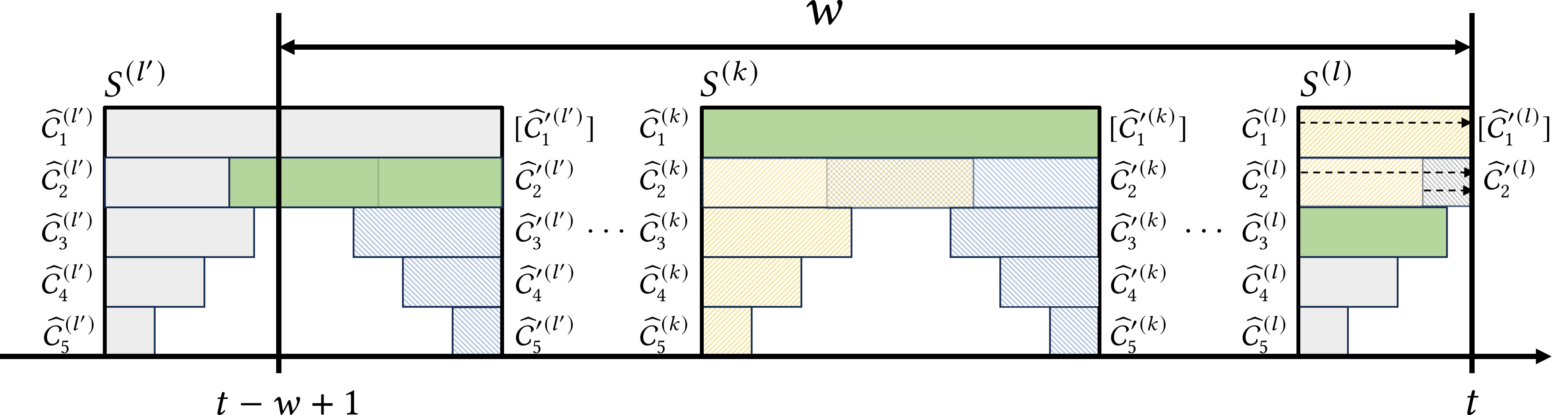
Figure 1. Overview of the DPSW-Sketch framework.

framework

4.1. Algorithm Description

We illustrate the structure of the DPSW-Sketch framework in Figure 1. Generally, DPSW-Sketch partitions the prefix $S_{t}$ of the stream $S$ at any time $t$ into non-overlapping substreams $S^{(1)},\dots,$ $S^{(l)}$ of equal length. Then, based on the idea of smooth histogram (Braverman and Ostrovsky, 2007), we establish two lists of checkpoints in each substream and build a PCMS w.r.t. each checkpoint. For one list (in yellow), a PCMS is built from the beginning of the substream to each checkpoint. For the other list (in blue), a PCMS is constructed from each checkpoint to the end of the substream. To reduce space usage, we only keep PCMSs built in substreams that overlap with $W_{t}$, as expired items are irrelevant to queries on $W_{t}$. Finally, to process any query, we combine the results obtained from one PCMS per substream (in green), so that the concatenation of the items on which they are built is closest to $W_{t}$.

Algorithm 2 DPSW-Sketch Construction

Stream $S$, window size $w\in\mathbb{Z}^{+}$, privacy budget $\rho>0$, framework factors $\alpha,\beta\in(0,1)$, sketching parameters $\zeta,\eta\in(0,1)$DPSW-Sketch$\widehat{\mathcal{C}}_{t}$at time $t$

1:Initialize $I,I^{\prime}\leftarrow\emptyset$ and $l\leftarrow 0$ Pre-specify the indices of checkpoints in each substream $i=\lceil w^{\beta}\rceil$ to $1$

2:Append a new index $i$ to the end of $I$ $j=1$ to $|I|-2$

3:Find the largest $k>j$ such that $I[k]\geq(1-\alpha)\cdot I[j]$

4:Delete all indices between $j$ and $k$ (exclusive) from $I$ and renumber the remaining indices accordingly $j=1$ to $|I|$

5:Append an index $\lceil w^{\beta}\rceil-I[j]+1$ as $I^{\prime}[j]$ Sketch update w.r.t. an item $s_{t}\in S$ $t=1$ to $n$ $t=1$ or $|S^{(l)}|\geq\lceil w^{\beta}\rceil$

6:$l\leftarrow l+1$ and start a new substream $S^{(l)}$

7:Build a PCMS $\widehat{\mathcal{C}}^{(l)}_{1}$ with $\zeta,\eta$, and $\rho_{1}=\rho(2\alpha-\alpha^{2})$ between $t$ and $v^{(l)}_{1}=t+\lceil w^{\beta}\rceil-1$ $j=2$ to $|I|$

8:Build a PCMS $\widehat{\mathcal{C}}^{(l)}_{j}$ with $\zeta,\eta$ and $\rho_{j}=\rho\alpha^{j-2}(1-\alpha)^{3}/2$ between $t$ and $v^{(l)}_{j}=t+I[j]-1$

9:Build a PCMS $\widehat{\mathcal{C}}^{\prime(l)}_{j}$ with $\zeta,\eta$ and $\rho_{j}=\rho\alpha^{j-2}(1-\alpha)^{3}/2$ between $u^{(l)}_{j}=t+I^{\prime}[j]$ and $t+\lceil w^{\beta}\rceil-1$ $j=1$ to $|I|$

10:if $v^{(l)}_{j}\geq t$ then $\widehat{\mathcal{C}}^{(l)}_{j}$.add$(s_{t})$

11:if $j>1$ and $u^{(l)}_{j}\leq t$ then $\widehat{\mathcal{C}}^{\prime(l)}_{j}$.add$(s_{t})$

12:Find the smallest $l^{\prime}<l$ with $S^{(l^{\prime})}\cap W_{t}\neq\emptyset$ and delete all PCMSs built on $S^{(l^{\prime}-1)}$ and previous substreams

13:Use the union of PCMSs on $S^{(l^{\prime})},\dots,S^{(l)}$ as $\widehat{\mathcal{C}}_{t}$ at time $t$

Sketch Construction

The detailed procedure to construct DPSW-Sketch over the sliding window is presented in Algorithm 2. Generally, DPSW-Sketch uses two factors $\alpha,\beta\in(0,1)$ to determine its structure: $\alpha$ controls the number of checkpoints in each substream and $\beta$ specifies the size of each substream as $\lceil w^{\beta}\rceil$. The first step in the construction process is to pre-specify a list $I$ of indices of checkpoints from $\lceil w^{\beta}\rceil$ to $1$ following the maintenance procedure of smooth histogram with the smooth factor $\beta$ (Braverman and Ostrovsky, 2007). The resultant list $I$ has two properties: (1) $I$ contains as few checkpoints as possible ($|I|=O(\frac{\log{w}}{\alpha})$ according to (Braverman and Ostrovsky, 2007)); and (2) it guarantees that for any two neighboring checkpoints $I[k],I[k-1]$ ($k=2,\dots,|I|$), $I[k]$ must be either at least $(1-\alpha)\cdot I[k-1]$ or $I[k-1]-1$. Then, we reverse each index in $I$ to obtain the other set $I^{\prime}$ of indices. As such, we use each checkpoint in $I$ or $I^{\prime}$ to indicate the end point of a PCMS that starts from the beginning of a substream or the start point of a PCMS that finishes at the end of a substream, respectively, both relative to the beginning of the substream.

After obtaining $I$ and $I^{\prime}$, the algorithm proceeds to maintain the sketch framework when receiving a new item $s_{t}$ in the stream $S$ at time $t$ ($t=1,\dots,n$). When the first item is received or the current substream is full, we start a new substream $S^{(l)}$, initialize two sets $\widehat{\mathcal{C}}^{(l)},\widehat{\mathcal{C}}^{\prime(l)}$ of PCMSs within $S^{(l)}$ according to $I$ and $I^{\prime}$, and allocate the private budget $\rho$ among the PCMSs. Since the first indices in $I$ and $I^{\prime}$ both correspond to the entire substream, we build only one PCMS for them. Additionally, we allocate higher privacy budgets to PCMSs maintained on more items to reduce total estimation errors. Subsequently, the framework is updated by adding the current item $s_{t}$ to all PCMSs in $\widehat{\mathcal{C}}^{(l)}$ and $\widehat{\mathcal{C}}^{\prime(l)}$ whose corresponding ranges contain $s_{t}$, each following Lines 1–2 of Algorithm 1. Finally, we check whether there is any obsolete substream, where all items come before the beginning of $W_{t}$ and are irrelevant to the statistics on $W_{t}$ and in the future, and remove all PCMSs within them from the framework. After that, the union of all PCMSs in substreams that overlap with $W_{t}$ serves as the sketch $\widehat{\mathcal{C}}_{t}$ at time $t$.

Query Processing

The methods to compute the results for frequency estimation and heavy-hitter identification on $W_{t}$ using DPSW-Sketch are presented in Algorithm 3. To obtain the frequency of a query item $e$ in $W_{t}$, the algorithm finds and queries one PCMS within each substream that overlaps with $W_{t}$. For any intermediate substream that is fully covered by $W_{t}$, the PCMS w.r.t. the whole substream is selected. For the first substream that might contain expired items, it chooses the PCMS that starts before, but is closest to, the beginning of $W_{t}$. Similarly, for the current substream, it identifies the PCMS that is closest to $t$ and has already been completed. Finally, the estimated frequency $\widehat{f}_{e,t}$ of item $e$ on $W_{t}$ is the sum of frequencies queried from all selected PCMSs according to Lines 3–5 of Algorithm 1. The method can also be extended to find an (approximate) set of $\gamma$-heavy hitters for a threshold $\gamma\in(0,1)$. It first queries the frequency $\widehat{f}_{e,t}$ of each item $e\in\mathcal{E}$ according to Lines 1-5. Then, each item $e\in\mathcal{E}$ is checked one by one: If $\widehat{f}_{e,t}$ is greater than or equal to $(\gamma-\zeta)w$, $e$ will be added to $\widehat{\mathcal{H}}_{\gamma,t}$. After processing all items, $\widehat{\mathcal{H}}_{\gamma,t}$ is returned for the heavy-hitter query.

Algorithm 3 DPSW-Sketch Query Processing

DPSW-Sketch$\widehat{\mathcal{C}}_{t}$at time $t$, window size $w\in\mathbb{Z}^{+}$, item $e\in\mathcal{E}$(for frequency query) or threshold $\gamma\in(0,1)$(for heavy-hitter query) (Approximate) frequency $\widehat{f}_{e,t}$or set $\widehat{\mathcal{H}}_{\gamma,t}$of $\gamma$-heavy hitters Frequency query on item $e\in\mathcal{E}$using DPSW-Sketch

1:$x\leftarrow\operatorname*{arg\,max}_{1\leq j\leq|I|}u^{(l^{\prime})}_{j}\leq\max(t-w+1,1)$

2:$y\leftarrow\operatorname*{arg\,max}_{1\leq j\leq|I|}v^{(l)}_{j}\leq t$

3:$\widehat{f}_{e}^{(l^{\prime})}\leftarrow\widehat{\mathcal{C}}^{\prime(l)}_{x}$.query$(e)$ and $\widehat{f}_{e}^{(l)}\leftarrow\widehat{\mathcal{C}}^{(l)}_{y}$.query$(e)$ $k=l^{\prime}+1$ to $l-1$

4:$\widehat{f}_{e}^{(k)}\leftarrow\widehat{\mathcal{C}}^{(k)}_{1}$.query$(e)$

5:$\widehat{f}_{e,t}\leftarrow\sum_{k=l^{\prime}}^{l}\widehat{f}_{e}^{(k)}$ Heavy-hitter query using DPSW-Sketch

6:Initialize $\widehat{\mathcal{H}}_{\gamma,t}\leftarrow\emptyset$ $e\in\mathcal{E}$

7:Compute $\widehat{f}_{e,t}$ as Lines 1–5

8:if $\widehat{f}_{e,t}\geq(\gamma-\zeta)w$ then $\widehat{\mathcal{H}}_{\gamma,t}\leftarrow\widehat{\mathcal{H}}_{\gamma,t}\cup\{e\}$

9:$\widehat{\mathcal{H}}_{\gamma,t}$

4.2. Theoretical Analysis

We first provide a formal privacy guarantee for DPSW-Sketch.

Lemma 4.1.

DPSW-Sketch $\widehat{\mathcal{C}}_{t}$ at any time $t$ constructed by Algorithm 2 satisfies $\rho$-zCDP.

Proof.

According to (Zhao et al., 2022, Theorem 3.1), each PCMS in $\widehat{\mathcal{C}}_{t}$ satisfies zCDP w.r.t. the privacy parameter with which it is initialized. That is, for any $k\geq 1$, $\widehat{\mathcal{C}}^{(k)}_{1}$ provides $\rho_{1}$-zCDP, where $\rho_{1}=\rho(2\alpha-\alpha^{2})$; $\widehat{\mathcal{C}}^{(k)}_{j}$ and $\widehat{\mathcal{C}}^{\prime(k)}_{j}$ provide $\rho_{j}$-zCDP, where $\rho_{j}=\rho\alpha^{j-2}(1-\alpha)^{3}/2$, for each $j=2,\ldots,|L|$. Since all of these PCMSs are built in the same substream $S^{(k)}$, their total privacy cost $\rho_{all}$ is calculated by applying the adaptive composition of zCDP as:

$$\rho_{all}=\rho(2\alpha-\alpha^{2})+2\sum_{j=2}^{|L|}\frac{\rho}{2}\alpha^{j-2}(1-\alpha)^{3}=\rho-\rho(1-\alpha)^{2}+\rho(1-\alpha)^{2}(1-\alpha^{|L|-1})<\rho.$$

Consequently, the output in each substream consisting of the union of all PCMSs satisfies $\rho$-zCDP. Finally, since all substreams are mutually disjoint, DPSW-Sketch $\widehat{\mathcal{C}}_{t}$ at any time $t$ built by Algorithm 2 satisfies $\rho$-zCDP due to the parallel composition of zCDP. ∎

According to (Zhao et al., 2022), a PCMS can only guarantee zCDP for queries. That is, it assumes that an adversary has no access to the internal sketch structure and is allowed to query a PCMS after the PCMS has been built on all items in the dataset. As such, any query can be regarded as a post-processing step without additional privacy losses. DPSW-Sketch follows the same setting as (Zhao et al., 2022): By dividing the stream into disjoint substreams and using smooth histograms to pre-specify the range in which each PCMS is built, we ensure that all PCMSs are queried only after they have been built without updates. Therefore, DPSW-Sketch can answer an unlimited number of queries at all times with DP. We consider how to convert $\rho$-zCDP to $(\varepsilon,\delta)$-DP according to Theorem 3.2. Specifically, to guarantee $(\varepsilon,\delta)$-DP for any $\varepsilon>0$ and $\delta\in(0,1)$, the value of $\rho$ is set as:

(1) $$\rho=\varepsilon+2\ln(1/\delta)-2\sqrt{\varepsilon\ln(1/\delta)+\ln^{2}(1/\delta)}.$$

Next, we analyze the error of the DPSW-Sketch framework for frequency estimation.

Lemma 4.2.

The frequency $\widehat{f}_{e,t}$ by Algorithm 3 satisfies $\Pr\big{[}|\widehat{f}_{e,t}-f_{e,t}|\leq\zeta w+\xi\big{]}\geq 1-O(\sqrt{w}\eta)$, where $\xi=O\big{(}\sqrt{w}(\zeta+\frac{1}{\sqrt{\rho}}\log\frac{1}{\zeta\eta})\big{)}$.

Proof.

We compute the error bound of $\widehat{f}_{e,t}$ for estimating $f_{e,t}$ by summing the upper bounds of its errors in all substreams. For each substream $S^{(k)}$ ($l^{\prime}<k<l$) that is fully covered by $W_{t}$, we always obtain $\widehat{f}^{(k)}_{e}$ from $\widehat{\mathcal{C}}^{(k)}_{1}$. According to Theorem 3.3, we have

(2) $$\Pr\big{[}|\widehat{f}^{(k)}_{e}-f^{(k)}_{e}|\leq\zeta\cdot\lceil w^{\beta}\rceil+\xi^{(k)}\big{]}\geq 1-\eta,$$

where $\xi^{(k)}=\sqrt{\frac{2\log(2/\eta)}{\rho(2\alpha-\alpha^{2})}}\cdot\sqrt{\log\big{(}\frac{4\log(2/\eta)}{\zeta\eta}\big{)}}$. For $S^{(l^{\prime})}$ and $S^{(l)}$ that partially overlap with $W_{t}$, the errors come from the estimates of PCMSs and the misalignments between $W_{t}$ and the ranges of the PCMSs used for query processing. Specifically, we have

(3) $$\Pr\big{[}|\widehat{f}^{(l^{\prime})}_{e}-f^{(l^{\prime})}_{e}|\leq(\alpha+\zeta)\cdot I[x]+\xi^{(l^{\prime})}\big{]}\geq 1-\eta;$$

(4) $$\Pr\big{[}|\widehat{f}^{(l)}_{e}-f^{(l)}_{e}|\leq(\alpha+\zeta)\cdot I[y]+\xi^{(l)}\big{]}\geq 1-\eta,$$

where $\xi^{(l^{\prime})}=\sqrt{\frac{2\log(2/\eta)}{\rho_{x}}}\cdot\sqrt{\log\big{(}\frac{4\log(2/\eta)}{\zeta\eta}\big{)}}$ and $\xi^{(l)}=\sqrt{\frac{2\log(2/\eta)}{\rho_{y}}}\cdot\sqrt{\log\big{(}\frac{4\log(2/\eta)}{\zeta\eta}\big{)}}$. Since there are at most $l-l^{\prime}+1\leq\lceil w^{1-\beta}\rceil+1$ active substreams, by combining Eqs. 2–4 and applying the union bound and the triangle inequality, we obtain with probability at least $1-(\lceil w^{1-\beta}\rceil+1)\eta$,

(5) $$|\widehat{f}_{e,t}-f_{e,t}|\leq\sum_{k=l^{\prime}}^{l}|\widehat{f}^{(k)}_{e}-f^{(k)}_{e}|\leq\sum_{k=l^{\prime}+1}^{l-1}\Big{(}\zeta\lceil w^{\beta}\rceil+\xi^{(k)}\Big{)}+(\alpha+\zeta)(I[x]+I[y])+\xi^{(l^{\prime})}+\xi^{(l)}.$$

Taking $\beta=\frac{1}{2}$ and $\alpha=O(1)$, Eq. 5 can be simplified as

$$|\widehat{f}_{e,t}-f_{e,t}|\leq\zeta w+O\Big{(}\sqrt{w}\big{(}\zeta+\frac{1}{\sqrt{\rho}}\log\frac{1}{\zeta\eta}\big{)}\Big{)},$$

because $\xi^{(k)}=O\big{(}\frac{1}{\sqrt{\rho}}\log\frac{1}{\zeta\eta}\big{)}$ for each $k\in[l^{\prime},\dots,l]$ and $I[x]=I[y]=O(\sqrt{w})$, and the proof is concluded. ∎

Then, we extend the error bound to heavy-hitter identification.

Lemma 4.3.

The set $\widehat{\mathcal{H}}_{\gamma,t}$ returned by Algorithm 3 satisfies (1) for any item $e\in\mathcal{E}$ with $f_{e,t}\geq\gamma w+O\big{(}\sqrt{w}(\zeta+\frac{1}{\sqrt{\rho}}\log\frac{1}{\zeta\eta})\big{)}$, $e\in\widehat{\mathcal{H}}_{\gamma,t}$ with probability at least $1-O(m\sqrt{w}\eta)$; (2) for any item $e\in\mathcal{E}$ with $f_{e,t}<(\gamma-2\zeta)w-O\big{(}\sqrt{w}(\zeta+\frac{1}{\sqrt{\rho}}\log\frac{1}{\zeta\eta})\big{)}$, $e\notin\widehat{\mathcal{H}}_{\gamma,t}$ with probability at least $1-O(m\sqrt{w}\eta)$.

Proof.

According to Lemma 4.2, for any item $e\in\mathcal{E}$ with $f_{e,t}\geq\gamma w+\xi$, where $\xi=O\big{(}\sqrt{w}(\zeta+\frac{1}{\sqrt{\rho}}\log\frac{1}{\zeta\eta})\big{)}$, we have $\widehat{f}_{e,t}\geq f_{e,t}-\zeta w-\xi\geq(\gamma-\zeta)w$ and $e$ is included in $\widehat{\mathcal{H}}_{\gamma,t}$ with probability $1-O(\sqrt{w}\eta)$. Similarly, for any item $e\in\mathcal{E}$ with $f_{e,t}<(\gamma-2\zeta)w-\xi$, we have $\widehat{f}_{e,t}\leq f_{e,t}+\zeta w+\xi<(\gamma-\zeta)w$ and $e$ is not included in $\widehat{\mathcal{H}}_{\gamma,t}$ with probability $1-O(\sqrt{w}\eta)$. By applying the union bound w.r.t. all the $m$ items in $\mathcal{E}$, it guarantees that the above results hold for all items with probability at least $1-O(m\sqrt{w}\eta)$. ∎

Finally, the main theoretical results of the DPSW-Sketch framework are summarized as follows.

Theorem 4.4.

For any window size $w$, framework factors $\beta=\frac{1}{2}$ and $\alpha=O(1)$, sketching parameters $\zeta,\eta\in(0,1)$, privacy parameters $\varepsilon>0$ and $\delta\in(0,1)$, the following results hold:

1. DPSW-Sketch is $(\varepsilon,\delta)$-differentially private.

2. It provides an $\Big{(}O\big{(}\zeta w+\frac{\sqrt{w\log(1/\delta)}}{\varepsilon}\log\frac{wm}{\zeta\eta}\big{)},\eta\Big{)}$-approximate frequency $\widehat{f}_{e,t}$ for each item $e\in\mathcal{E}$.

3. It gives an $\Big{(}O\big{(}\zeta\sqrt{w}+\frac{\sqrt{w\log(1/\delta)}}{\varepsilon}\log\frac{wm}{\zeta\eta}\big{)},\eta\Big{)}$-approximate set $\widehat{\mathcal{H}}_{\gamma,t}$ of $\gamma$-heavy hitters for any threshold $\gamma\geq 4\zeta$.

4. It uses $O(\frac{\sqrt{w}\log{w}}{\zeta}\log\frac{wm}{\eta})$ space and $O(\log{w}\log\frac{wm}{\eta})$ time per update and processes a frequency query and a heavy-hitter query in $O(\sqrt{w}\log\frac{wm}{\eta})$ and $O(m\sqrt{w}$ $\log\frac{wm}{\eta})$ time.

Proof.

First of all, by setting the value of $\rho$ according to Eq. 1 for any given $\varepsilon>0$ and $\delta\in(0,1)$, DPSW-Sketch satisfies $(\varepsilon,\delta)$-DP. Eq. 1 implies $\frac{1}{\rho}=\frac{\varepsilon+2\ln(1/\delta)+2\sqrt{\varepsilon\ln(1/\delta)+\ln^{2}(1/\delta)}}{\varepsilon^{2}}=O\big{(}\frac{\log(1/\delta)}{\varepsilon^{2}}\big{)}$. By replacing $\frac{1}{\rho}$ with $O\big{(}\frac{\log(1/\delta)}{\epsilon^{2}}\big{)}$ and scaling $\eta$ to $O(\frac{\eta}{m\sqrt{w}})$ for each PCMS in Lemmas 4.2 and 4.3, we obtain the approximation bounds for frequency estimation and heavy-hitter identification.

In terms of space complexity, we can see that there exist $O(\sqrt{w})$ active substreams that overlap with $W_{t}$ for any $t\in\mathbb{Z}^{+}$, the number of PCMSs maintained in each active substream is $O(\log w)$, and the size of each PCMS is $O(\frac{1}{\zeta}\log\frac{wm}{\eta})$. In total, the space complexity of DPSW-Sketch is $O(\frac{\sqrt{w}\log{w}}{\zeta}\log\frac{wm}{\eta})$. In terms of time complexity, we can see that Algorithm 2 uses $O(\sqrt{w})$ time to decide the two lists of checkpoints in a smooth histogram, initializes $O(\log w)$ PCMSs at the beginning of each substream, inserts an item into at most $O(\log w)$ PCMSs, and requires $O(\log\frac{wm}{\eta})$ hash computations and counter updates for each insertion. Since the checkpoints are computed only once before stream processing, the (amortized) time complexity per update is $O(\log{w}\log\frac{wm}{\eta})$. For a frequency query, Algorithm 3 selects $O(\sqrt{w})$ PCMSs from DPSW-Sketch and takes $O(\log\frac{wm}{\eta})$ time to query each PCMS. Thus, the time complexity of each frequency query is $O(\sqrt{w}\log\frac{wm}{\eta})$. A heavy-hitter query requires to perform $m$ frequency queries and thus has a time complexity of $O(m\sqrt{w}\log\frac{wm}{\eta})$. ∎

Comparison with Existing Private Sketches in (Chan et al., 2012; Upadhyay, 2019; Blocki et al., 2023)

We show how the theoretical results of DPSW-Sketch improve over those of the existing private sliding-window sketches (Chan et al., 2012; Upadhyay, 2019; Blocki et al., 2023). First, the sketches in (Chan et al., 2012; Upadhyay, 2019; Blocki et al., 2023) are all specific to the identification of heavy hitters and the estimation of their frequencies with bounded errors, while DPSW-Sketch can approximate the frequencies of all items. Second, DPSW-Sketch either provides better approximations for heavy-hitter identification or has a lower space complexity than the sketches in (Chan et al., 2012; Upadhyay, 2019; Blocki et al., 2023). Compared to PCC-MG in (Chan et al., 2012), which requires $O(w)$ space for an additive error of $O(\sqrt{w})$, and U-Sketch in (Upadhyay, 2019), which has an additive error of $\tilde{O}(w^{3/4})$ in $\tilde{O}(\sqrt{w})$ space, the additive error and space complexity of DPSW-Sketch are both $\tilde{O}(\sqrt{w})$. BLMZ-Sketch (Blocki et al., 2023) achieves the same $\tilde{O}(\sqrt{w})$ additive error as DPSW-Sketch. However, its update time and space usage, both of which are $O(\frac{\sqrt{w}\log^{4}{w}}{\varepsilon\gamma})$, are much higher than those of DPSW-Sketch. Finally, we note that all private sketches have higher errors and use more space than non-private sketches in the sliding window model, e.g., (Gou et al., 2020; Wu et al., 2023), due to the noise added to satisfy DP.

5. Experiments

In this section, we conducted extensive experiments on five real-world and synthetic datasets to evaluate the performance of DPSW-Sketch compared to the state-of-the-art baselines.

Table 2. Dataset Information

Dataset	$n$	$m$	Description
AOL	10.7M	38,411	Web search query logs
MovieLens	25M	62,423	Movie ratings
WorldCup	1.3B	82,592	Web server logs
Gaussian	10M	25,600	Synthetic Gaussian-distributed items
Zipf	10M	25,600	Synthetic Zipf-distributed items

Datasets

We employed three real-world and two synthetic datasets in the experiments. Their statistics are reported in Table 2, where $n$ is the dataset size and $m$ is the domain size. For synthetic datasets, the skewness parameter for the Zipf distribution is $1$; the mean and standard deviation of the Gaussian distribution are $50$ and $25$, respectively. More detailed information on these datasets is provided in Appendix A due to space limitations.

Baselines

We adopted U-Sketch (Upadhyay, 2019), PCC-MG (Chan et al., 2012), and BLMZ-Sketch (Blocki et al., 2023) as baselines for frequency estimation and heavy-hitter identification with DP in the sliding window model. We also used a non-private sliding-window sketch, Microscope-Sketch (Wu et al., 2023), as a baseline to measure “the price of privacy.” More details about these baselines are also deferred to Appendix B.

Implementation

All the algorithms we compared were implemented in C++ and compiled with the “-O3” flag. We ran each experiment with a single thread on a server with an Intel Xeon Gold 6428 processor @2.5GHz and 32GB RAM. For each baseline, we either used the implementation published by the original authors or followed the idea of the original paper for implementation and fine-tuned the parameters. We set the window size $w$ to $10^{6}$ by default. The default parameters in DPSW-Sketch are as follows: (1) number of checkpoints $|I|=3$; (2) length of each substream $0.1w$; and (3) height $a\in[2,\dots,5]$ and width $b\in[500,\dots,5000]$ for each PCMS. The parameter sensitivity of DPSW-Sketch is further analyzed in Appendix C.

Metrics

The query workload on each dataset was generated by randomly sampling $1\%$ timestamps from time $t=w$ to $n$ and performing a set of $100$ frequency queries and a heavy-hitter query at each sampled timestamp. We divided the items into two groups according to their ground-truth frequencies as high- and low-frequency items (top-$50$ most frequent vs. all remaining items) and each set $\mathcal{Q}$ of queries has an equal number of items from each group. The following metrics are used for performance evaluation:

• Mean Absolute Error (MAE), $\frac{1}{|\mathcal{Q}|}\sum_{e\in\mathcal{Q}}|\widehat{f}_{e,t}-f_{e,t}|$, is used to measure the performance for frequency queries.

• Mean Relative Error (MRE), $\frac{1}{|\mathcal{Q}|}\sum_{e\in\mathcal{Q}}\frac{|\widehat{f}_{e,t}-f_{e,t}|}{f_{e,t}}$, is also used to measure the performance for frequency queries.

• F1-score, which is the harmonic mean of the precision score, i.e., the ratio of $|\widehat{\mathcal{H}}_{e,t}\cap\mathcal{H}_{e,t}|$ to $|\widehat{\mathcal{H}}_{e,t}|$, and the recall score, i.e., the ratio of $|\widehat{\mathcal{H}}_{e,t}\cap\mathcal{H}_{e,t}|$ to $|\mathcal{H}_{e,t}|$, is used to measure the performance for heavy-hitter queries.

• Throughput, i.e., the average number of items to insert per second (in Kops), and Sketch Size (in KB) are used to measure the time and space efficiency of each method.

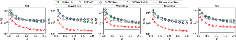
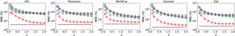
Figure 2. Performance for frequency queries on high-frequency items by varying privacy parameter $\varepsilon\in\{0.1,0.2,0.4,\dots,2.0\}$.

experiments

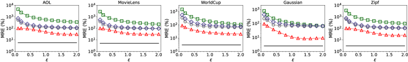
Figure 3. Performance for frequency queries on low-frequency items by varying privacy parameter $\varepsilon\in\{0.1,0.2,0.4,\dots,2.0\}$.

experiments

5.1. Frequency Estimation

Figures 2 and 3 illustrate the performance of different sketches for frequency queries on high- and low-frequency items by varying the privacy parameter $\varepsilon$ from $0.1$ to $2$. For sketches satisfying $(\varepsilon,\delta)$-DP and $\rho$-zCDP, we fix $\delta$ to $1/n^{1.5}$ and compute the value of $\rho$ according to Eq. 1. Here, we restrict the selection of low-frequency items to those with frequencies of at least 100. This is because PCC-MG and BLMZ-Sketch, which use Misra-Gries sketches (Misra and Gries, 1982) as building blocks, cannot answer queries on low-frequency items. For the above query workload, PCC-MG and BLMZ-Sketch still do not report the results for many frequency queries. In such cases, we treat their results as $0$ in the calculation of MAE and MRE.

Our results show that the MAEs and MREs of all sketches, except (non-private) Microscope-Sketch, generally decrease with increasing $\varepsilon$ in all datasets. For both high- and low-frequency items, DPSW-Sketch achieves significantly lower MAE and MRE than all other private sketches across different values of $\varepsilon$. Especially, DPSW-Sketch is the only method among them whose MREs are always within $10\%$ for high-frequency items and $100\%$ for low-frequency items when $\varepsilon\geq 1$. The results confirm that DPSW-Sketch strikes a better balance between frequency estimation accuracy and privacy than state-of-the-art private sketches in the sliding-window model.

Furthermore, U-Sketch, PCC-MG, and BLMZ-Sketch generally exhibit performance similar to each other on high-frequency items, and PCC-MG is slightly better when $\varepsilon$ is smaller, while U-Sketch becomes better for a larger value of $\varepsilon$. For low-frequency items, U-Sketch sometimes performs much worse than PCC-MG and BLMZ-Sketch because its estimation errors are even higher than simply treating all missing frequencies as $0$. In all datasets, the three private baselines always have at least $4\times$ higher MAE and $2\times$ higher MRE than those of DPSW-Sketch. Finally, the performance of all private sketches for frequency estimation is not comparable to that of the state-of-the-art non-private sketch, Microscope-Sketch, especially on low-frequency items, because (1) they introduce substantial noise in the counters to satisfy DP and (2) their sketch structures are modified for ease of privacy accounting, which further leads to estimation errors due to the misalignment between the sliding window and the sketch used for query processing.

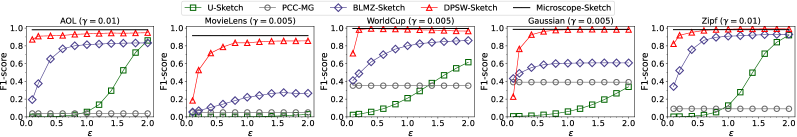
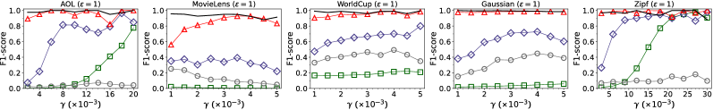
Figure 4. Performance for heavy-hitter queries by varying privacy parameter $\varepsilon$ and threshold $\gamma$.

experiments

5.2. Heavy-Hitter Identification

Figure 4 shows the performance of different sketches for heavy-hitter identification by varying the privacy parameter $\varepsilon$ when the threshold $\gamma=0.005$ or $0.01$ and the threshold $\gamma$ when $\varepsilon=1$. We observe that DPSW-Sketch achieves higher F1-scores than other DP sketches in almost all cases. Its performance is mostly close to that of (non-private) Microscope-Sketch when $\varepsilon\geq 1$. These results verify its good trade-off between accuracy for heavy-hitter identification and privacy. The performance of BLMZ-Sketch and U-Sketch improves with increasing $\varepsilon$. However, they are inferior to DPSW-Sketch due to much larger noise. The F1-score of PCC-MG remains constant for all values of $\varepsilon$. This is because PCC-MG is built directly on MG sketches, which only guarantee to return heavy hitters but cannot filter out non-heavy hitters. As such, it has achieved a recall score of $1$ when $\varepsilon=0.1$ (i.e., no false negatives) while inevitably including some false positives in all its results, regardless of the value of $\varepsilon$. In contrast, BLMZ-Sketch only uses MG sketches for pre-screening and builds additional counters to decide whether a candidate item is a heavy hitter, thus achieving better performance for heavy-hitter queries.

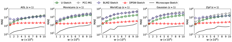
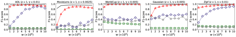
Figure 5. Performance of different sketches for frequency and heavy-hitter queries by varying window size $w$.

experiments

5.3. Performance vs. Window Size

Figure 5 presents the performance of different sketches for frequency and heavy-hitter queries by varying the window size $w$ from $10^{5}$ to $10^{6}$. We observe that DPSW-Sketch has better query accuracies than other private sketches in almost all cases across different window sizes. The MAEs of DPSW-Sketch for frequency estimation increase with the window size $w$. This can be attributed to a greater number of distinct elements within a larger window, which leads to more hash collisions. Note that the MAEs grow much lower than $w$ and thus the MREs of DPSW-Sketch drop with increasing $w$. Furthermore, the F1-scores of DPSW-Sketch for heavy-hitter queries also increase with $w$. Therefore, the performance of DPSW-Sketch generally degrades in smaller windows. This is because the variance of Gaussian noise added to PCMSs is nearly independent of $w$. As such, queries in smaller windows are more severely disturbed by noise than those in larger windows.

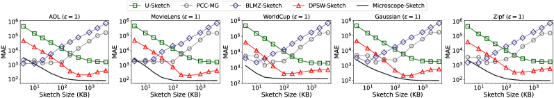
Figure 6. Performance of different sketches for frequency and heavy-hitter queries by varying sketch size from 4KB to 4MB.

experiments

5.4. Space and Time Efficiency

Figure 6 illustrates the performance of different sketches for frequency and heavy-hitter queries when their sizes range from 4KB to 4MB and $\varepsilon=1$. We observe that for CMS-based methods, i.e., U-Sketch, DPSW-Sketch, and Microscope-Sketch, their query performance first decreases with increasing sketch sizes and then becomes steady when the sketch sizes are sufficiently large because larger sketches naturally lead to fewer hash collisions and more accurate counters. On the contrary, MG sketch-based methods, i.e., PCC-MG and BLMZ-Sketch, generally perform better when their sketch sizes are smaller because larger sketches introduce much more noise while having little benefit.

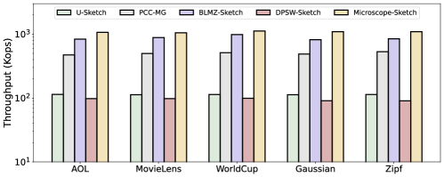
Figure 7. Throughput of each sketch in the default setting.

experiments

Figure 7 presents the throughputs of different sketches in the default setting (i.e., for $\varepsilon=1$ and $w=10^{6}$ with all the sketch parameters fine-tuned). DPSW-Sketch has a throughput of about 100Kops (i.e., processing 100K items per second) across all datasets, which satisfies the requirement for real-world stream processing and is similar to that of U-Sketch. However, Microscope-Sketch, BLMZ-Sketch, and PCC-MG have higher throughputs (500–1000Kops) than DPSW-Sketch. For Microscope-Sketch, this is because it utilizes a more efficient structure without considering privacy. For BLMZ-Sketch and PCC-MG, this can be attributed to the fact that MG sketches are much smaller than CMSs.

6. Conclusion

In this paper, we propose DPSW-Sketch, a novel sketch framework for frequency and heavy-hitter queries with event-level differential privacy (DP) in the sliding-window model. Theoretically, DPSW-Sketch satisfies DP, provides results for both queries within bounded errors, and has sublinear time and space complexities w.r.t. the size of the sliding window. These results improve upon those of existing private sliding-window sketches. Experimental results also indicate that DPSW-Sketch achieves better trade-offs between utility and privacy than state-of-the-art baselines.

In future work, we would like to extend DPSW-Sketch to satisfy more rigorous notions of DP, such as user-level DP and local DP (LDP). We are also interested in the design of private federated sketches for distributed data streams.

Appendix A Dataset Information

We describe the datasets used in our experiments and the pre-processing steps applied to them below.

• AOL comprises 36,389,567 web queries over three months in the AOL website. Each record has several fields such as AnonID, Query, QueryTime, ItemRank, and ClickURL. We pre-processed the dataset as follows: (1) removing all duplicate and incomplete records; (2) sorting the records by QueryTime; (3) acquiring keywords from the Query field of each record after stopword removal and lemmatization; (4) filtering out typos and meaningless keywords. After all pre-processing steps, the dataset contains 10,710,880 items with 38,411 unique query keywords. We aim to keep track of the number of times each keyword is queried and the top trending keywords in the latest $w$ queries.

• MovieLens consists of 25,000,095 ratings on 62,423 movies contributed by 162,541 users from January 1995 to November 2019. Each record contains fields such as userId, movieId, rating, and timestamp. The original data set has been sorted chronologically without missing fields. We extract the movieId field for statistics to track the number of times each movie is rated and the most popular movies in the latest $w$ user interactions.

• WorldCup encompasses all 1,352,804,107 requests made to the 1998 FIFA World Cup website from April 30, 1998 to July 26, 1998. Each request has the following fields: timestamp, clientID, objectID, size, method, status, type, and server. Pre-processing steps include (1) removing incomplete and duplicate requests and (2) sorting the requests by timestamp. After pre-processing, the dataset contains 1,267,670,951 requests for 82,592 distinct URLs. We aim to track the number of times each URL is requested and the top trending URLs in the latest $w$ requests.

• Gaussian is a synthetic dataset consisting of 10,000,000 items with a domain size of 25,600, in which 95% items are drawn from a Gaussian distribution with mean $\mu=50$ and standard deviation $\sigma=25$ (negative numbers are ignored) and rounded to the nearest positive integers, and the remaining 5% items are drawn from a discrete uniform distribution in the range $[1,25600]$.

• Zipf is also a synthetic dataset consisting of 10,000,000 items with a domain size of 25,600, in which 95% items are drawn from a Zipf distribution with the skewness parameter $1$ and the remaining 5% items are drawn from a discrete uniform distribution in the range $[1,25600]$.

We illustrate the distribution of item frequencies in the above five datasets in Figure 8, where each point $(x,y)$ in a plot denotes that the ratio of the number of items with a frequency of at least $x$ and the number of items in the domain is $y$.

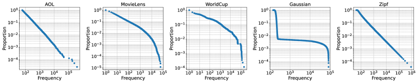
Figure 8. Distribution of item frequencies in each dataset.

appendix

Appendix B Baseline Implementation

In the following, we provide some implementation details of different sketches in the experiments.

• PCC-MG (Chan et al., 2012): There is no publicly available implementation of PCC-MG. Thus, we follow the specifications in (Chan et al., 2012) to implement PCC-MG. Given a parameter $\lambda\in(0,1)$, it builds a binary tree with $l=\lceil\ln\frac{4}{\lambda}\rceil$ levels, each of which consists of equal-length and disjoint blocks. For each block at the $i^{th}$ level, a (private) Misra-Gries sketch is constructed with the privacy parameter $\varepsilon_{i}=\frac{\varepsilon}{2^{l-i+1}}$ and the sketch parameter $\lambda_{i}=\frac{1}{2^{i}(l+1)}$. In each experiment, we test different values of $\lambda$ and report the best result achieved by PCC-MG among all values of $\lambda$.

• U-Sketch (Upadhyay, 2019): To the best of our knowledge, U-Sketch has not been implemented for experimentation. We first tried to reproduce U-Sketch following the specifications in (Upadhyay, 2019). However, this leads to large sketch sizes (typically several times the size of the sliding window), which is deemed unacceptable for stream processing. Therefore, we implement U-Sketch based on the general idea of (Upadhyay, 2019) but modify the parameter setting. To reduce space usage, we divide the sliding window into $100$ blocks and limit the number of sketches built in each block to $2$. Other parameters are fine-tuned for the best performance in each experiment.

• BLMZ-Sketch (Blocki et al., 2023): To the best of our knowledge, BLMZ-Sketch has also not been implemented for experimentation. We found that the specifications in (Blocki et al., 2023) imply an excessively small block size (even less than $1$ in some cases). Therefore, similar to U-Sketch, we implement BLMZ-Sketch based on the general idea of (Blocki et al., 2023) but modify the parameter setting. In particular, we fix the number $l$ of levels to $4$ and the size of each block to $\frac{w}{16}$. Other parameters are determined accordingly, and, in each experiment, we also fine-tune them and report the best result among all tested settings.

• Microscope-Sketch (Wu et al., 2023): We use the code published by the authors on GitHub. We test the variants of Microscope-Sketch using CMS, CU-Sketch, and CountSketch and find that the CMS version shows the best performance in most cases. Therefore, we only employ its CMS version in our experiments. Finally, in each experiment, we also report the best result among all parameter settings.

Appendix C Parameter Sensitivity

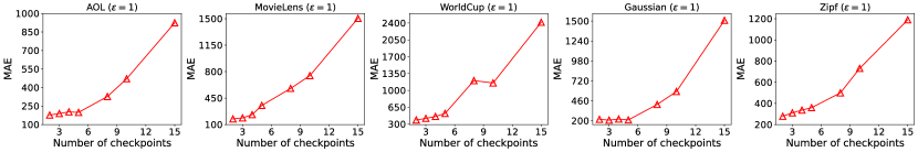
Figure 9. Effect of the number of checkpoints in each smooth histogram on the performance of DPSW-Sketch.

appendix

Figure 9 illustrates how the number of checkpoints in each smooth histogram affects the MAE for frequency estimation and throughput of DPSW-Sketch. By setting the privacy parameter $\varepsilon$ to $1$ and the length of each sub-stream to $0.1w$ and limiting the total sketch size to at most 100KB, we adjust the value of $\alpha$ from $0.99$ to $0.1$ so that $|I|$ is varied over $\{2,3,4,5,8,10,15\}$. Our results indicate a significant growth in MAE across all datasets as the number of checkpoints increases. This is because more checkpoints lead to fewer privacy budgets assigned to all PCMSs. Accordingly, larger Gaussian noise should be added to each counter, which naturally causes higher MAEs. Meanwhile, the throughput of DPSW-Sketch drops nearly linearly with the number of checkpoints since each item should be added to at most $2|I|-1$ PCMSs. Therefore, we set the number of checkpoints $|I|$ to $3$ in the remaining experiments.

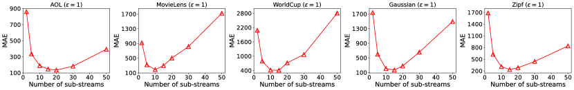
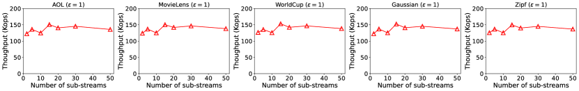
Figure 10. Effect of the number of sub-streams in each window on the performance of DPSW-Sketch.

appendix

Figure 10 illustrates the impact of the number of sub-streams in each window on the MAE of frequency estimation and throughput of DPSW-Sketch. We fix $\varepsilon=1$ and $|I|=3$ and limit the total sketch size to at most 100KB. We then vary the value of $\beta$ to adjust the length of each sub-stream from $0.02w$ to $0.5w$. Consequently, the number of sub-streams in each window is set to $\{2,5,10,15,20,30,50\}$. We find that, as the number of sub-streams increases, the MAE first decreases, reaching its lowest point around $10$ sub-streams per window, and then increases. On the one hand, when the length of a sub-stream is too large, the high MAE is caused by the misalignment between the current window and the sketch used for query processing. On the other hand, when the length of a sub-stream is too small, the limitation on the total sketch size requires that the size of each PCMS is smaller, leading to more hash collisions and a higher MAE. The throughput is almost not affected by the number of sub-streams, as DPSW-Sketch only updates the PCMSs built in the latest sub-stream. Therefore, we set the length of each sub-stream to $0.1w$ in the remaining experiments.

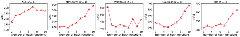
Figure 11. Effect of the number of hash functions in each PCMS on the performance of DPSW-Sketch.

appendix

Figure 11 shows how the values of $a$ and $b$ for each PCMS affect the MAE for frequency estimation and throughput of DPSW-Sketch. We also fix $\varepsilon=1$, $|I|=3$, and the length of each sub-stream to $0.1w$. Then, by limiting the total sketch size to 100KB, we vary the number $a$ of hash functions in each PCMS from $2$ to $10$ and, accordingly, the range of each hash function from $5,000$ to $1,000$. The results show that no single value of $a$ guarantees good performance in all datasets because each dataset has a different frequency distribution of items and domain size. The throughput decreases almost linearly as the number of hash functions increases as each PCMS updates $a$ counters per item. Since the MAE does not decrease when $a>5$ in most datasets, we only test $a=2,3,4,5$ for high throughput and present the best result among them in each experiment.

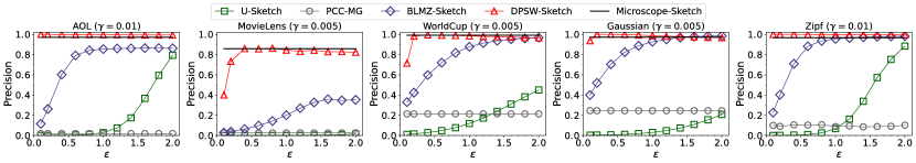
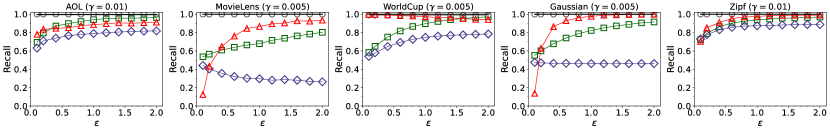
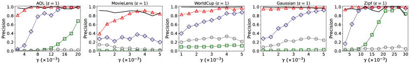
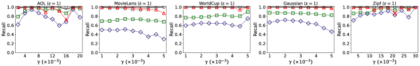
Figure 12. Precision and recall scores for heavy-hitter identification by varying privacy parameter $\varepsilon$ and threshold $\gamma$.

appendix

Appendix D Supplemental Experiments

Precision and Recall for Heavy-Hitter Identification

To complement the experimental results in Section 5.2, we provide the precision and recall scores of different sketches for heavy-hitter identification by varying the privacy parameter $\varepsilon$ and the threshold $\gamma$ in Figure 12 following the same settings as used in Figure 4. These results further verify the outstanding performance of DPSW-Sketch for heavy-hitter identification, as it simultaneously achieves higher precision and recall scores than BLMZ-Sketch and U-Sketch. We also confirm that PCC-MG does not achieve high F1-scores due to extremely low precision scores, although it always has a recall score of $1$. Finally, all methods have relatively low performance for heavy-hitter identification in the MovieLens dataset. This is due to concept drift: as new trending movies always emerge over time, the set of heavy hitters in the MovieLens dataset continuously evolves. For comparison, item frequencies are almost independent of time in synthetic datasets; although trending keywords and URLs also change over time in the AOL and WorldCup datasets, they are quite stable relative to the length of the sliding window. Since none of the compared methods explicitly considers the issue of concept drift, they cannot achieve as high performance in the MovieLens dataset as in other datasets. We leave the problems of detecting changes in data distribution and taking into account concept drift in heavy-hitter identification with privacy concerns for future work.

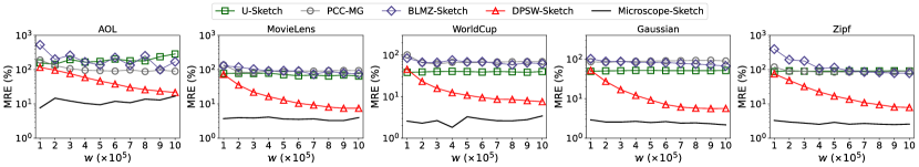
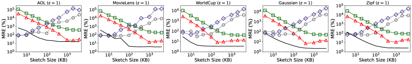
Figure 13. MRE for frequency estimation by varying window size and sketch size.

appendix

MRE with Varying Window Size and Sketch Size

We present the MRE of each sketch for frequency estimation by varying the window size and the sketch size in Figure 13, following the same setting as used in Figures 5 and 6. We observe similar trends as described in Sections 5.3 and 5.4.

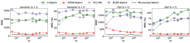
Figure 14. MAE and MRE for frequency estimation by varying domain size $m$.

appendix

Effect of Domain Size

Figure 14 illustrates the impact of the domain size $m$ on the MAE and MRE for frequency estimation in the two synthetic datasets. We generate Gaussian and Zipf datasets of 10M items with domain sizes ranging from $400$ to $409,600$ following the procedure in Appendix A. The results indicate that the MAE for all methods remains relatively stable across different domain sizes. DPSW-Sketch and Microscope-Sketch exhibit stability in MAE and MRE for different domain sizes, with DPSW-Sketch consistently outperforming other differentially private baselines and closely matching the performance of Microscope-Sketch. Generally, DPSW-Sketch shows strong scalability against the dimensionality of the datasets.

References

- (1)
- Andersson and Pagh (2023) Joel Daniel Andersson and Rasmus Pagh. 2023. A Smooth Binary Mechanism for Efficient Private Continual Observation. Advances in Neural Information Processing Systems 36 (2023), 49133–49145.
- Arasu and Manku (2004) Arvind Arasu and Gurmeet Singh Manku. 2004. Approximate Counts and Quantiles over Sliding Windows. In Proceedings of the Twenty-Third ACM SIGMOD-SIGACT-SIGART Symposium on Principles of Database Systems (PODS ’04). Association for Computing Machinery, New York, NY, USA, 286–296.
- Ben-Basat et al. (2016) Ran Ben-Basat, Gil Einziger, Roy Friedman, and Yaron Kassner. 2016. Heavy hitters in streams and sliding windows. In IEEE INFOCOM 2016 - The 35th Annual IEEE International Conference on Computer Communications. IEEE, 1–9.
- Ben-Eliezer et al. (2022) Omri Ben-Eliezer, Dan Mikulincer, and Ilias Zadik. 2022. Archimedes Meets Privacy: On Privately Estimating Quantiles in High Dimensions Under Minimal Assumptions. Advances in Neural Information Processing Systems 35 (2022), 32450–32464.
- Blocki et al. (2023) Jeremiah Blocki, Seunghoon Lee, Tamalika Mukherjee, and Samson Zhou. 2023. Differentially Private -Heavy Hitters in the Sliding Window Model. In The Eleventh International Conference on Learning Representations. OpenReview.net.
- Braverman and Ostrovsky (2007) Vladimir Braverman and Rafail Ostrovsky. 2007. Smooth Histograms for Sliding Windows. In 48th Annual IEEE Symposium on Foundations of Computer Science. IEEE, 283–293.
- Bun and Steinke (2016) Mark Bun and Thomas Steinke. 2016. Concentrated Differential Privacy: Simplifications, Extensions, and Lower Bounds. In Theory of Cryptography - 14th International Conference, TCC 2016-B, Beijing, China, October 31-November 3, 2016, Proceedings, Part I. Springer, Berlin, Heidelberg, 635–658.
- Chan et al. (2012) T.-H. Hubert Chan, Mingfei Li, Elaine Shi, and Wenchang Xu. 2012. Differentially Private Continual Monitoring of Heavy Hitters from Distributed Streams. In Privacy Enhancing Technologies - 12th International Symposium, PETS 2012, Vigo, Spain, July 11-13, 2012, Proceedings. Springer, Berlin, Heidelberg, 140–159.
- Chan et al. (2011) T.-H. Hubert Chan, Elaine Shi, and Dawn Song. 2011. Private and Continual Release of Statistics. ACM Transactions on Information and System Security 14, 3, Article 26 (2011), 24 pages.
- Charikar et al. (2004) Moses Charikar, Kevin C. Chen, and Martin Farach-Colton. 2004. Finding frequent items in data streams. Theoretical Computer Science 312, 1 (2004), 3–15.
- Cormode et al. (2012) Graham Cormode, Minos N. Garofalakis, Peter J. Haas, and Chris Jermaine. 2012. Synopses for Massive Data: Samples, Histograms, Wavelets, Sketches. Foundations and Trends in Databases 4, 1-3 (2012), 1–294.
- Cormode and Muthukrishnan (2005) Graham Cormode and S. Muthukrishnan. 2005. An improved data stream summary: the count-min sketch and its applications. Journal of Algorithms 55, 1 (2005), 58–75.
- Datar et al. (2002) Mayur Datar, Aristides Gionis, Piotr Indyk, and Rajeev Motwani. 2002. Maintaining Stream Statistics over Sliding Windows. SIAM J. Comput. 31, 6 (2002), 1794–1813.
- Dwork et al. (2006a) Cynthia Dwork, Krishnaram Kenthapadi, Frank McSherry, Ilya Mironov, and Moni Naor. 2006a. Our Data, Ourselves: Privacy Via Distributed Noise Generation. In Advances in Cryptology – EUROCRYPT 2006. Springer, Berlin, Heidelberg, 486–503.
- Dwork et al. (2006b) Cynthia Dwork, Frank McSherry, Kobbi Nissim, and Adam D. Smith. 2006b. Calibrating Noise to Sensitivity in Private Data Analysis. In Theory of Cryptography. Springer, Berlin, Heidelberg, 265–284.
- Dwork et al. (2010) Cynthia Dwork, Moni Naor, Toniann Pitassi, and Guy N. Rothblum. 2010. Differential privacy under continual observation. In Proceedings of the 42nd ACM Symposium on Theory of Computing (STOC ’10). Association for Computing Machinery, New York, NY, USA, 715–724.
- Epasto et al. (2023) Alessandro Epasto, Jieming Mao, Andres Munoz Medina, Vahab Mirrokni, Sergei Vassilvitskii, and Peilin Zhong. 2023. Differentially Private Continual Releases of Streaming Frequency Moment Estimations. In 14th Innovations in Theoretical Computer Science Conference (ITCS 2023). Schloss Dagstuhl – Leibniz-Zentrum für Informatik, Dagstuhl, Germany, 48:1–48:24.
- Estan and Varghese (2002) Cristian Estan and George Varghese. 2002. New directions in traffic measurement and accounting. In Proceedings of the 2002 Conference on Applications, Technologies, Architectures, and Protocols for Computer Communications (SIGCOMM ’02). Association for Computing Machinery, New York, NY, USA, 323–336.
- Fichtenberger et al. (2023) Hendrik Fichtenberger, Monika Henzinger, and Jalaj Upadhyay. 2023. Constant Matters: Fine-grained Error Bound on Differentially Private Continual Observation. In Proceedings of the 40th International Conference on Machine Learning. PMLR, 10072–10092.
- Ghazi et al. (2023) Badih Ghazi, Ravi Kumar, Jelani Nelson, and Pasin Manurangsi. 2023. Private Counting of Distinct and k-Occurring Items in Time Windows. In 14th Innovations in Theoretical Computer Science Conference (ITCS 2023). Schloss Dagstuhl – Leibniz-Zentrum für Informatik, Dagstuhl, Germany, 55:1–55:24.
- Gillenwater et al. (2021) Jennifer Gillenwater, Matthew Joseph, and Alex Kulesza. 2021. Differentially Private Quantiles. In Proceedings of the 38th International Conference on Machine Learning. PMLR, 3713–3722.
- Google (2024) Google. 2024. How Google retains data we collect. https://policies.google.com/technologies/retention.
- Gou et al. (2020) Xiangyang Gou, Long He, Yinda Zhang, Ke Wang, Xilai Liu, Tong Yang, Yi Wang, and Bin Cui. 2020. Sliding Sketches: A Framework using Time Zones for Data Stream Processing in Sliding Windows. In Proceedings of the 26th ACM SIGKDD International Conference on Knowledge Discovery & Data Mining (KDD ’20). Association for Computing Machinery, New York, NY, USA, 1015–1025.
- Haug et al. (2022) Johannes Haug, Alexander Braun, Stefan Zürn, and Gjergji Kasneci. 2022. Change Detection for Local Explainability in Evolving Data Streams. In Proceedings of the 31st ACM International Conference on Information & Knowledge Management (CIKM ’22). Association for Computing Machinery, New York, NY, USA, 706–716.
- Hehir et al. (2023) Jonathan Hehir, Daniel Ting, and Graham Cormode. 2023. Sketch-Flip-Merge: Mergeable Sketches for Private Distinct Counting. In Proceedings of the 40th International Conference on Machine Learning. PMLR, 12846–12865.
- Huang et al. (2022) Ziyue Huang, Yuan Qiu, Ke Yi, and Graham Cormode. 2022. Frequency Estimation Under Multiparty Differential Privacy: One-shot and Streaming. Proceedings of the VLDB Endowment 15, 10 (2022), 2058–2070.
- Kaplan et al. (2022) Haim Kaplan, Shachar Schnapp, and Uri Stemmer. 2022. Differentially Private Approximate Quantiles. In Proceedings of the 39th International Conference on Machine Learning. PMLR, 10751–10761.
- Lebeda and Tetek (2023) Christian Janos Lebeda and Jakub Tetek. 2023. Better Differentially Private Approximate Histograms and Heavy Hitters using the Misra-Gries Sketch. In Proceedings of the 42nd ACM SIGMOD-SIGACT-SIGAI Symposium on Principles of Database Systems (PODS ’23). Association for Computing Machinery, New York, NY, USA, 79–88.
- Melis et al. (2016) Luca Melis, George Danezis, and Emiliano De Cristofaro. 2016. Efficient Private Statistics with Succinct Sketches. In 23rd Annual Network and Distributed System Security Symposium (NDSS ’16). The Internet Society, 15 pages.
- Mir et al. (2011) Darakhshan J. Mir, S. Muthukrishnan, Aleksandar Nikolov, and Rebecca N. Wright. 2011. Pan-private algorithms via statistics on sketches. In Proceedings of the Thirtieth ACM SIGMOD-SIGACT-SIGART Symposium on Principles of Database Systems (PODS ’11). Association for Computing Machinery, New York, NY, USA, 37–48.
- Misra and Gries (1982) Jayadev Misra and David Gries. 1982. Finding Repeated Elements. Science of Computer Programming 2, 2 (1982), 143–152.
- Muthukrishnan (2005) S. Muthukrishnan. 2005. Data Streams: Algorithms and Applications. Foundations and Trends in Theoretical Computer Science 1, 2 (2005), 117–236.
- Pagh and Thorup (2022) Rasmus Pagh and Mikkel Thorup. 2022. Improved Utility Analysis of Private CountSketch. Advances in Neural Information Processing Systems 35 (2022), 25631–25643.
- Papapetrou et al. (2012) Odysseas Papapetrou, Minos N. Garofalakis, and Antonios Deligiannakis. 2012. Sketch-based Querying of Distributed Sliding-Window Data Streams. Proceedings of the VLDB Endowment 5, 10 (2012), 992–1003.
- Perrier et al. (2019) Victor Perrier, Hassan Jameel Asghar, and Dali Kaafar. 2019. Private Continual Release of Real-Valued Data Streams. In 26th Annual Network and Distributed System Security Symposium (NDSS ’19). The Internet Society, 13 pages.
- Rivetti et al. (2015) Nicolo Rivetti, Yann Busnel, and Achour Mostéfaoui. 2015. Efficiently Summarizing Data Streams over Sliding Windows. In 2015 IEEE 14th International Symposium on Network Computing and Applications. IEEE, 151–158.
- Smith et al. (2020) Adam D. Smith, Shuang Song, and Abhradeep Thakurta. 2020. The Flajolet-Martin Sketch Itself Preserves Differential Privacy: Private Counting with Minimal Space. Advances in Neural Information Processing Systems 33 (2020), 19561–19572.
- Upadhyay (2019) Jalaj Upadhyay. 2019. Sublinear Space Private Algorithms Under the Sliding Window Model. In Proceedings of the 36th International Conference on Machine Learning. PMLR, 6363–6372.
- Wang et al. (2022) Lun Wang, Iosif Pinelis, and Dawn Song. 2022. Differentially Private Fractional Frequency Moments Estimation with Polylogarithmic Space. In The Tenth International Conference on Learning Representations. OpenReview.net.
- Wu et al. (2023) Yuhan Wu, Shiqi Jiang, Siyuan Dong, Zheng Zhong, Jiale Chen, Yutong Hu, Tong Yang, Steve Uhlig, and Bin Cui. 2023. MicroscopeSketch: Accurate Sliding Estimation Using Adaptive Zooming. In Proceedings of the 29th ACM SIGKDD Conference on Knowledge Discovery and Data Mining (KDD ’23). Association for Computing Machinery, New York, NY, USA, 2660–2671.
- Yildirim et al. (2020) Sinan Yildirim, Kamer Kaya, Soner Aydin, and Hakan Bugra Erentug. 2020. Differentially Private Frequency Sketches for Intermittent Queries on Large Data Streams. In 2020 IEEE International Conference on Big Data. IEEE, 4083–4092.
- Zhao et al. (2022) Fuheng Zhao, Dan Qiao, Rachel Redberg, Divyakant Agrawal, Amr El Abbadi, and Yu-Xiang Wang. 2022. Differentially Private Linear Sketches: Efficient Implementations and Applications. Advances in Neural Information Processing Systems 35 (2022), 12691–12704.
- Zhong et al. (2021) Zheng Zhong, Shen Yan, Zikun Li, Decheng Tan, Tong Yang, and Bin Cui. 2021. BurstSketch: Finding Bursts in Data Streams. In Proceedings of the 2021 International Conference on Management of Data (SIGMOD ’21). Association for Computing Machinery, New York, NY, USA, 2375–2383.
- Zhu et al. (2020) Wennan Zhu, Peter Kairouz, Brendan McMahan, Haicheng Sun, and Wei Li. 2020. Federated Heavy Hitters Discovery with Differential Privacy. In Proceedings of the Twenty Third International Conference on Artificial Intelligence and Statistics. PMLR, 3837–3847.