Reduced Basis method for finite volume simulations of parabolic PDEs
applied to porous media flows

Abstract

Numerical simulations are a highly valuable tool to evaluate the impact of the uncertainties of various model parameters, and to optimize e.g. injection-production scenarios in the context of underground storage (of CO₂ typically). Finite volume approximations of Darcy’s parabolic model for flows in porous media are typically run many times, for many values of parameters like permeability and porosity, at costly computational efforts.

We study the relevance of reduced basis methods as a way to lower the overall simulation cost of finite volume approximations to Darcy’s parabolic model for flows in porous media for different values of the parameters such as permeability. In the context of underground gas storage (of CO₂ typically) in saline aquifers, our aim is to evaluate quickly, for many parameter values, the flux along some interior boundaries near the well injection area—regarded as a quantity of interest—. To this end, we construct reduced bases by a standard POD-Greedy algorithm. Our POD-Greedy algorithm uses a new goal-oriented error estimator designed from a discrete space-time energy norm independent of the parameter. We provide some numerical experiments that validate the efficiency of the proposed estimator.

Keywords
single-phase flow, porous media, finite volumes, reduced basis, goal-oriented error estimate

Mathematics subject classification
35J50, 65M08, 65N15, 76S05

1 Introduction

In the context of geological storage of gases such as CO₂, computational models of single phase Darcy flow are useful to optimize the efficiency of injection, and to quantify uncertainties with a view to assessing the enduring stability of the storage site. As concerns CO₂, it is usually injected in underground storage sites such as depleted oil and gas reservoirs or saline aquifers in sedimentary basins. In this work, we are mainly interested in the case of saline aquifers.

In saline aquifers, the numerical simulation of single phase Darcy flows is very meaningful, in particular in a large domain at basin scale where it is computationally costly. Indeed, brine is moved by the gas (CO₂) injected outside the storage area. In risk assessment studies, one needs to evaluate the pressure field in the surrounding aquifer (typically along faults far from the storage domain) many times, for many values of the uncertain parameters . Quantifying the impact of the uncertainties of model parameters, on the time evolution of the flux at underground boundaries of the storage area, is also desired to optimize the injection process. For both purposes and given values of the model parameters, the flow simulator computes the solution of a large linear system many times. This multi-query setting induces costly computational efforts especially for large domains. To lower the overall simulation cost of computations at many parameter values, we consider a Reduced Basis (RB) approach.

Many other methods have been proposed to reduce the time calculations in basin modeling and reservoir simulation. For instance, in case of LGR methods, the grid is locally refined only in a region of interest depending on the local solution properties, whereas in other areas, where the solution is relatively smooth or uniform, grid cells can be larger, leading to a smaller computational cost. Likewise, the Adaptive Mesh Refinement (AMR) method [29, 4] divides the computational domain into a hierarchy of grids and each grid is refined or coarsened by considering an error estimate as the simulation progresses.

In this work, our approach consists rather in considering a reduced basis (RB) approach to replace many calls to a parametrized High-Fidelity (HF) simulator at many parameter values, by calls to a less expensive Low-Fidelity (LF) surrogate model with a certification of the error.

A RB procedure relies on an existing computational model, a parametrized HF simulator which can provide one with numerical approximations of the model solutions at fixed parameter values. When the HF model consists in large linear systems (one at each time step in a nonstationary flow simulation e.g.), a LF (reduced) computational model is usually constructed by Galerkin projection of the HF model onto a linear subspace.

In the context of porous media flows, the choice of the appropriate numerical scheme to discretize the governing equations in space is crucial to obtain a consistent approximation of the fluxes. Finite-difference [26, 5], finite-volume [15] or finite-element [11, 14] methods have been classically used in industrial contexts such as reservoir engineering. In particular the finite-volume two-point flux approximation is a reference method in this field because of its simplicity and its stability properties (the discrete operator turns out to be an M-matrix). However, once the grids are not $\mathbf{\Lambda}$-orthogonal , this scheme is no more consistent. Over the past years, new discretization methods have been proposed to satisfy this property: multi-point flux approximations [1], mimetic finite-differences [6], virtual elements [3], hybrid [16] or vertex-centred finite-volumes [17] to quote just a few of them. We also mention non-linear schemes [23, 24, 27] that were designed in order to obtain monotone approximations and properties such as the positivity of the solutions or the maximum principle on these grids. In this work, we consider the average multi-point flux approximation (MPFA-FV) method which was for instance studied in [27]. That approximation does not preserve the positivity of the solutions or the maximum principle, but it is consistent on grids that are not $\mathbf{\Lambda}$-orthogonal.

In the present work, given a parametrized HF model that discretizes Darcy’s parabolic model by a MPFA-FV method resulting in a time-series of (large) linear systems, see Section 2, we then standardly construct a parametrized LF model by projecting (the pressure field solution to) Darcy flows at each time step, whatever the parameter value, onto one (single) linear subspace by Galerkin method.

To that aim, we adopt a standard two-stage procedure [18, 21]. First, in a costly offline stage, we identify a linear approximation space spanned by (snapshots of) simulations at relevant parameter values. During this stage, HF simulations with many degrees of freedom $\mathcal{N}$ (several thousands of cells) are run at least $\mathsf{N}$ times, $\mathsf{N}$ being the dimension of the linear approximation space. During the offline stage, a LF reduced computational model is also numerically constructed. Next, in an online stage, the values of solutions and the quantities of interests at yet-unexplored parameter values are evaluated numerically using the LF (reduced) computational model, if possible with a computational complexity independent from $\mathcal{N}$.

The offline selection of a good linear subspace for Galerkin projection is crucial to the quality of the LF model, i.e. to control the approximation error of the LF model with respect to the HF model at every parameter values. Regarding the applications of the RB method to parametrized HF simulator that are based on (finite-volume discretizations of) parabolic PDEs, a standard selection technique is the POD-Greedy method based on a reliable a posteriori error estimation, see e.g. [21].

In the present work, we propose new a posteriori error estimators. Like e.g. [21], our a posteriori error estimators evaluate the approximation by a LF model of a HF model discretizing parabolic PDEs by the finite volume method (a MPFA-FV discretization in our application case to single phase Darcy flows). However, by contrast with standard RB literature, we use a discrete space-time energy norm of $L^{2}([0,T];H^{1}(\Omega))$-type that is independent from the parameter. We also provide goal-oriented estimators for a linear QOI, like in [18, 20] (where a parametrized HF model based on finite element approximations is reduced using another algorithm than POD-Greedy to construct the LF model).

To assess the accuracy of our error estimate, and the performance of our new certified RB approach (i.e. the dimension of the reduced LF model in a multi-query scenario for monophasic Darcy flows parametrized by the permeability), we also perform numerical simulations.

Our HF model based on MPFA-FV discretization is non-affine in the permeability parameter: we use the Empirical Interpolation Method (EIM) [25, 10] for the construction of a LF model independent from $\mathcal{N}$. Moreover, to construct a lower bound of the coercivity constant (required by a rigorous error estimation) we use the Successive Constraint Method (SCM) [12, 22]. It is noteworthy that, for accurate a posteriori error estimation taking care of machine precision, we numerically compute quadratic-in-the-parameter forms (in the dual norm of the residual) as in [7], using a specific orthonormal basis to represent the residual, while a traditional offline/online decomposition [8] leads to numerical precision issues.

Our numerical results show that the proposed a posteriori error estimation guarantees a reliable evaluation of a single-phase Darcy flow model and accurately quantify the solution error. We also proved that the goal-oriented estimation for a given linear QOI offers for a small dimension of the reduced model a very good precision for the output error.

This paper is outlined as follows. In Section 2, we present a discretization of single-phase flow (SPF) equations in porous media based on the multi-point flux approximation that defines our HF numerical model. Section 3 discusses the concept of a goal-oriented method applied to the SPF problem. We derive the a posteriori error estimation for the primal and dual problems as well as for the output model. We also present the POD-Greedy algorithm to construct the reduced basis. In Section 3.5, we additionally elaborate on the computation of the residual dual norm in order to avoid the impact of round-off errors on the error bound. We then numerically study the behavior and efficiency of the proposed estimate in Section 4. Finally, concluding remarks are given in Section 5.

2 A parametrized High-Fidelity model

In this section, we introduce the PDE modelling of single phase porous media flows, and its discretization by a finite volume method which defines our parametrized HF simulator in the sequel.

2.1 A Darcy model of single phase porous media flows

We consider the flow of a slightly compressible fluid saturating a porous rock within a connected and bounded polygonal domain $\Omega$ of $\mathbb{R}^{3}$ and a time $T>0$. The boundary $\partial\Omega=\Gamma_{{\color[rgb]{0,0,1}\rm D}}\cup\Gamma_{\rm N}$ of $\Omega$ is partitioned into a part where Dirichlet boundary conditions are applied, and a part where homogeneous Neumann boundary conditions are used.

The balance of the water volume combined with Darcy’s law and with initial and boundary data leads to

$$\phi c_{t}\partial_{t}p-\nabla\cdot(\mathbf{\Lambda}({\nabla}p+\rho g{\nabla}z)) =q, (0,T)\times\Omega,$$ in (2.1a)

$$\mathbf{\Lambda}({\nabla}p+\rho g{\nabla}z)\cdot\mathbf{n} =0, (0,T)\times\Gamma_{\mathrm{N}},$$ on (2.1b)

$$p =p_{\mathrm{D}}, (0,T)\times\Gamma_{\mathrm{D}},$$ on (2.1c)

$$p(x,t=0) =p^{0}(x), \Omega,$$ in (2.1d)

where $p$ denotes the fluid pressure, $\mathbf{\Lambda}=\overline{\kappa}/\mu$ the mobility tensor, $\overline{\kappa}$ the rock permeability tensor, $\mu$ the fluid viscosity, $\phi$ the rock porosity, $c_{t}$ the total compressibility, $\rho$ the fluid density, $g$ the gravity constant and $q(p)$ a well source term to be precised later (in Section 2.2 after discretization). We designate by $\mathbf{n}$ the unit normal vector outside the domain.

A typical multi-query setting (with parameter variations to be addressed by the RB method), occurs when the permeability tensor $\overline{\kappa}$ is uncertain. We here assume that the domain is made up of two areas, corresponding to two rock types (a reservoir one and a cap rock) each with constant isotropic permeabilities $\overline{\kappa}_{1}$ or $\overline{\kappa}_{2}$ (see e.g. Fig. 2.1) so that

$$\mathbf{\Lambda}=\begin{bmatrix}\Lambda&0&0\\ 0&\Lambda&0\\ 0&0&\Lambda\end{bmatrix}$$

where $\Lambda(x)=\sum_{i=1}^{2}\frac{\kappa_{i}}{\mu}\mathbb{1}_{(i)}(x)$ and $\mathbb{1}_{i}$ denotes the indicator function of the region $i$.

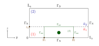
Figure 2.1: Typical domain configuration.

Throughout this work, we consider the storage area $(S)$ with boundaries

$$\Gamma_{\rm int}=\{y_{1}\}\times[0,z_{1}]\cup\{y_{2}\}\times[0,z_{1}]\cup[y_{1},y_{2}]\times\{z_{1}\},$$

where we seek to predict the time evolution of the flux $s$ defined by

$$s=-\int_{\Gamma_{\rm int}}\mathbf{\Lambda}({{\nabla}}p+\rho{g}{\nabla}z)\cdot\boldsymbol{\mathbf{n}}\,\mathrm{d}S$$ (2.2)

over $\Gamma_{\rm int}$ for many values of $\kappa_{1}$ and $\kappa_{2}$.

2.2 Finite volume discretization

The single-phase flow equations are first discretized in time using the implicit Euler method, next in space using a finite volume method. Choosing a constant time step

$$\Delta t=\frac{T}{N},\quad N\in\mathbb{N}^{*}\,,$$

we consider at each time iteration $n\in\{0,\ldots,N-1\}$ an approximation $p^{n+1}\approx p(t^{n+1})$ at $t^{n+1}=(n+1)\;\Delta t$ solution to

$$\phi c_{t}\frac{p^{n+1}-p^{n}}{\Delta t}-\nabla\cdot\left(\mathbf{\Lambda}(\nabla p^{n+1}+\rho g\nabla z)\right) =q^{n+1},$$ (2.3a)

$$\mathbf{\Lambda}(\nabla p^{n+1}+\rho g\nabla z)\cdot\mathbf{n} =0,$$ (2.3b)

$$p^{n+1} =p_{\mathrm{D}}.$$ (2.3c)

The space discretization is performed using an admissible mesh of $\Omega$, defined by a triplet $\mathcal{D}=(\mathcal{T},\mathcal{E},\mathcal{P})$ where :

• $\mathcal{T}$ is a finite set of non empty compact convex polygonal sub-domains of $\Omega$ (the set of cells), called control volumes such that $\overline{\Omega}=\bigcup\limits_{K\in\mathcal{T}}\overline{K}$. For all $K\in\mathcal{T}$, we denote by $\operatorname{m}_{K}>0$ its measure and set $\partial K\stackrel{{\scriptstyle\mathrm{def}}}{{=}}\overline{K}\setminus K$.

• $\mathcal{E}$ is a family of subsets of $\overline{\Omega}$ (the set of faces) such that for any $K\in\mathcal{T}$, there exists a subset $\mathcal{E}_{K}$ of $\mathcal{E}$ where $\partial K=\bigcup\limits_{\sigma\in\mathcal{E}_{K}}\sigma$. For any $(K,L)\in\mathcal{T}^{2}$ with $K\neq L$, either the $(d-1)$ Lebesgue measure of $\overline{K}\cap\overline{L}$ is 0 or $\overline{K}\cap\overline{L}=\overline{\sigma}$ for some $\sigma\in\mathcal{E}$, with $\sigma=K|L$ (an interior face). We denote by $\operatorname{m}_{\sigma}$ the $(d-1)$-dimensional measure of $\sigma$. The sets of inner and boundary faces are denoted by $\mathcal{E}_{\operatorname{int}}$ and $\mathcal{E}_{\operatorname{ext}}$ respectively.

• $\mathcal{P}=\{\mathbf{x}_{K}\}_{K\in\mathcal{T}}$ is a collection of points within $\Omega$ indexed by $\mathcal{T}$ (called the cell centers, not required to be the barycenters) s.t. $\mathbf{x}_{K}\in K$ and $K$ is star-shaped with respect to $\mathbf{x}_{K}$.

For each cell $K\in\mathcal{T}$ and face $\sigma\in\mathcal{E}_{K}$, $\mathbf{n}_{K,\sigma}$ denotes the unit vector normal to $\sigma$ and pointing outward to $K$. Additionally, for any cell $K\in\mathcal{T}$ and any function $\Phi$ belonging to $L^{1}(K)$, we define $\langle\Phi\rangle_{K}\stackrel{{\scriptstyle\mathrm{def}}}{{=}}\operatorname{m}_{K}^{-1}\int_{K}\Phi{\,\operatorname{d}}x$.

Given an admissible mesh, numerically computable approximations $p^{n}_{K}\approx\langle p^{n}\rangle_{K}$ are defined after space discretization by a finite volume method. We first integrate (2.3a) over a cell $K$ to obtain

$$\int_{K}\phi c_{t}\frac{p^{n+1}-p^{n}}{\Delta t}\,{\,\operatorname{d}}x-\int_{K}\nabla\cdot(\mathbf{\Lambda}(\nabla p^{n+1}+\rho g\nabla z))\,{\,\operatorname{d}}x=\int_{K}q^{n+1}\,{\,\operatorname{d}}x.$$ (2.4)

Applying Green’s formula, we can transform the first two integrals and recast (2.4) as

$$\operatorname{m}_{K}\phi_{K}c_{t}\frac{\langle p^{n+1}\rangle_{K}-\langle p^{n}\rangle_{K}}{\Delta t}-\int_{\partial K}\mathbf{\Lambda}(\nabla p^{n+1}+\rho g\nabla z)\cdot\mathbf{n}_{K}\,{\,\operatorname{d}}\mathcal{\gamma}=\int_{K}q^{n+1}\,{\,\operatorname{d}}x.$$ (2.5)

By decomposing the boundary $\partial K$ into faces, we get

$$\operatorname{m}_{K}c_{t}\phi_{K}\frac{\langle p^{n+1}\rangle_{K}-\langle p^{n}\rangle_{K}}{\Delta t}-\sum_{\sigma\in\mathcal{E}_{K}}\int_{\sigma}\mathbf{\Lambda}(\nabla p^{n+1}+\rho g\nabla z)\cdot\mathbf{n}_{K,\sigma}\,{\,\operatorname{d}}S=\int_{K}q^{n+1}\,{\,\operatorname{d}}x,$$

which leads one to consider the following numerical scheme

$$\operatorname{m}_{K}\phi_{K}c_{t}(p_{K}^{n+1}-p_{K}^{n})+\Delta t\sum_{\sigma\in\mathcal{E}_{K}}F_{K,\sigma}^{n+1}=\Delta t\operatorname{m}_{K}q_{K}^{n+1}$$ (2.6)

with numerical fluxes $F_{K,\sigma}^{n+1}\approx-\int_{\sigma}\mathbf{\Lambda}(\nabla p^{n+1}+\rho g\nabla z)\cdot\mathbf{n}_{K,\sigma}\,{\,\operatorname{d}}S$ and numerical source terms $q_{K}^{n+1}$ that allow for the numerical computation of $(p_{K}^{n+1})_{K\in\mathcal{T}}$ given $(p_{K}^{n})_{K\in\mathcal{T}}$.

The Peaceman model [13] is used here for the well source term $q_{K}^{n+1}=\operatorname{m}_{K}^{-1}\int_{K}q^{n+1}\,{\,\operatorname{d}}x$. We suppose that the well is vertical and the perforations are oriented in the z-direction. The well model is then given by

$$q_{K}^{n+1}=\mathtt{WI}_{K}(p_{bh}-p_{K}^{n+1}-\rho{g}(z_{bh}-z_{K})),$$ (2.7)

where $p_{bh}$ is the bottom hole pressure and $\mathtt{WI}_{K}$ is the Peaceman well index in a perforated cell $K$.

The flux -$\int_{\sigma}\mathbf{\Lambda}(\nabla p^{n+1}+\rho g\nabla z)\cdot\mathbf{n}_{K,\sigma}\,{\,\operatorname{d}}S$ is numerically approximated using the average multi-point flux scheme studied in [27]. For each interior edge $\sigma\in{\mathcal{E}}_{\rm int}$, with $\mathcal{T}_{\sigma}=\{K,L\}$ the approximated flux $F_{K,\sigma}^{n+1}$ is defined as a convex combination of two linear fluxes $\tilde{F}_{K,\sigma}^{n+1}$ and $\tilde{F}_{L,\sigma}^{n+1}$ such that

$$F_{K,\sigma}^{n+1}=\mu_{K,\sigma}\tilde{F}_{K,\sigma}^{n+1}-\mu_{L,\sigma}\tilde{F}_{L,\sigma}^{n+1},\qquad\text{ with }\;\;\mu_{K,\sigma}\geq 0,\quad\mu_{L,\sigma}\geq 0,\quad\mu_{K,\sigma}+\mu_{L,\sigma}=1.$$ (2.8)

A numerical flux formula as given by (2.8) is clearly conservative, i.e,

$$F_{K,\sigma}^{n+1}+F_{L,\sigma}^{n+1}=0.$$ (2.9)

To build the linear fluxes $\tilde{F}_{K,\sigma}^{n+1}$ in (2.8), we approximate the pressure gradient $\nabla p$ in the direction of the conormal vector $\langle\mathbf{\Lambda}\rangle_{K}\mathbf{n}_{K,\sigma}$ after expressing the conormal as a linear combination of the vectors $(\mathbf{x}_{\sigma^{\prime}}-\mathbf{x}_{K})_{\{\sigma^{\prime}\in\mathcal{S}_{K,\sigma}\}}$

$$\langle\mathbf{\Lambda}\rangle_{K}\mathbf{n}_{K,\sigma}\approx\sum_{\sigma^{\prime}\in\mathcal{S}_{K,\sigma}}\alpha_{K,\sigma\sigma^{\prime}}(\mathbf{x}_{\sigma^{\prime}}-\mathbf{x}_{K}).$$ (2.10)

The decomposition (2.10) is achieved numerically by means of an optimization procedure which aims at reducing the sum of the coefficients $\alpha_{K,\sigma\sigma^{\prime}}$ and the size of the stencil $\mathcal{S}_{K,\sigma}\stackrel{{\scriptstyle\mathrm{def}}}{{=}}\{\sigma^{\prime}\in\mathcal{E}_{K}\,\alpha_{K,\sigma\sigma^{\prime}}\not=0\}$ within $\mathcal{E}_{K}$ [28]. In (2.10), $\mathbf{x}_{\sigma}$ is not the face center but an harmonic averaging interpolation point

$$\mathbf{x}_{\sigma}=\omega_{K,{{\color[rgb]{0,0,0}\sigma}}}\mathbf{y}_{K}+\omega_{L,{{\color[rgb]{0,0,0}\sigma}}}\mathbf{y}_{L}+\frac{d_{K,\sigma}d_{L,\sigma}}{d_{L,\sigma}\tau_{K,\sigma}+d_{K,\sigma}\tau_{L,\sigma}}(\boldsymbol{\tau}_{K}^{\sigma}-\boldsymbol{\tau}_{L}^{\sigma})$$ (2.11)

where

$$\omega_{K,{{\color[rgb]{0,0,0}\sigma}}}=\frac{d_{L,\sigma}\tau_{K,\sigma}}{d_{L,\sigma}\tau_{K,\sigma}+d_{K,\sigma}\tau_{L,\sigma}},\quad\displaystyle\omega_{L,{{\color[rgb]{0,0,0}\sigma}}}=\frac{d_{K,\sigma}\tau_{L,\sigma}}{d_{L,\sigma}\tau_{K,\sigma}+d_{K,\sigma}\tau_{L,\sigma}},$$ (2.12)

$$\tau_{K,\sigma}=\mathbf{n}_{K,\sigma}\langle\mathbf{\Lambda}\rangle_{K}\mathbf{n}_{K,\sigma},\quad\tau_{L,\sigma}=\mathbf{n}_{L,\sigma}\langle\mathbf{\Lambda}\rangle_{L}\mathbf{n}_{L,\sigma},$$ (2.13)

$$\displaystyle\boldsymbol{\tau}_{K}^{\sigma}=(\mathbf{\Lambda}_{K}-\tau_{K,\sigma}\rm{Id})\mathbf{n}_{K,\sigma},\quad\boldsymbol{\tau}_{L}^{\sigma}=(\mathbf{\Lambda}_{L}-\tau_{L,\sigma}\rm{Id})\mathbf{n}_{L,\sigma},$$ (2.14)

$d_{K,\sigma}$, $d_{L,\sigma}$ are the distances of the cell centers to $\sigma$, $\mathbf{y}_{K}$, $\mathbf{y}_{L}$ their projection on $\sigma$ defined by (see Figure 2.2)

$$\mathbf{y}_{K}=\mathbf{x}_{K}+d_{K,\sigma}\mathbf{n}_{K,\sigma},\quad\mathbf{y}_{L}=\mathbf{x}_{L}+d_{L,\sigma}\mathbf{n}_{L,\sigma}.$$

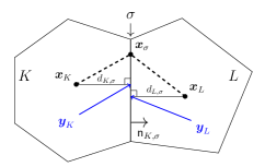
Figure 2.2: Harmonic averaging point.

The pressure trace at $\sigma\in\mathcal{E}_{K}$ is consistently reconstructed as

$$I_{\sigma}p=\sum_{M\in\{K,L\}}\!\omega_{M,\sigma}p_{M},\text{ where }\sum_{M\in\{K,L\}}\!\omega_{M,\sigma}=1,\qquad\omega_{M,\sigma}\geq 0,$$ (2.15)

using the same weights $\omega_{M,\sigma}$ as in (2.12) (for more details see [2]). With the previous approximations, the linear fluxes read

$$\tilde{F}_{K,\sigma}^{n+1}=\operatorname{m}_{\sigma}\sum_{\sigma^{\prime}\in\mathcal{S}_{K,\sigma}}\alpha_{K,\sigma\sigma^{\prime}}[(p^{n+1}+\rho gz)_{K,\sigma^{\prime}}-(p_{K}^{n+1}+\rho gz_{K})],$$ (2.16)

where we used the notation

$$(u)_{K,\sigma}=\begin{cases}I_{\sigma}u&\mbox{ if }\sigma=K|L,\\ u_{\sigma}&\mbox{ otherwise.}\end{cases}$$ (2.17)

Finally, to define the numerical flux $F_{K,\sigma}^{n+1}$, the weights $\mu_{K,\sigma}$ and $\mu_{L,\sigma}$ can be chosen in different ways. In this work, we set $\mu_{K,\sigma}=\mu_{L,\sigma}=\frac{1}{2}$ if $\sigma=K|L$ and $\mu_{K,\sigma}=1$ if $\sigma\subset\partial\Omega$. Let us remark that in (2.16), the average value of the boundary condition (2.1c) is used on the face $\sigma^{\prime}$ if $\sigma^{\prime}\subset\Gamma_{\rm D}$. An additional unknown $p_{\sigma^{\prime}}$ is added if $\sigma^{\prime}\subset\Gamma_{\rm N}$ which can be computed by adding the homogeneous Neumann condition to the discrete system, namely:

$$F_{K,\sigma}^{n+1}=0.$$

Our numerical output quantity of interest (QOI) $s$ is then defined as

$$s^{n+1}=\sum_{\begin{subarray}{c}\sigma=K|L\\ \sigma\subset\Gamma_{\rm int}\end{subarray}}F_{K,\sigma}^{n+1}.$$ (2.18)

Our HF model consists in the solutions of the $N$ discrete linear systems obtained after assembling equations (2.6) for all $K\in\mathcal{T}$, $n\in\{0,\ldots,N-1\}$

$$(\boldsymbol{M}+\Delta t\boldsymbol{A}){\boldsymbol{p}}_{\mathcal{M}}^{n+1}=\boldsymbol{M}{\boldsymbol{p}}_{\mathcal{M}}^{n}+\Delta t\,{\boldsymbol{b}},$$ (2.19)

see also (3.1) below, where

• $\boldsymbol{A}\in\mathbb{R}^{\mathcal{N}\times\mathcal{N}}$ is a matrix containing the terms $\alpha_{K,\sigma\sigma^{\prime}}$, with $\mathcal{N}=\rm{N_{c}}+{\rm N_{b}}$ ($\rm{N_{c}}$ is the total number of cells and ${\rm N_{b}}$ the number of boundaries where we have imposed Neumann boundary condition),

• $\boldsymbol{M}\in\mathbb{R}^{\mathcal{N}\times\mathcal{N}}$ is such that

  $$\boldsymbol{M}=\begin{bmatrix}\boldsymbol{M}_{\rm c}&\Large{0}\\ \Large{0}&\Large{0}\end{bmatrix},$$

  where $\boldsymbol{M}_{\rm c}\in\mathbb{R}^{\rm{N_{c}}\times\rm{N_{c}}}$ is a diagonal matrix made of the quantities $\operatorname{m}_{K}\phi_{K}c_{t}$,

• ${\boldsymbol{p}}_{\mathcal{M}}^{n+1}\in\mathbb{R}^{\mathcal{N}}$ is a vector composed of the values of the pressure $p^{n+1}$ in each element $K\in\mathcal{T}$ and on the edges $\sigma\subset\Gamma_{\rm N}\cap\partial K$,

• ${\boldsymbol{b}}\in\mathbb{R}^{\mathcal{N}}$ contains the Dirichlet condition values as well as the source terms $\mathcal{Q}_{K}^{n+1}$.

The QOI (2.18) can be rewritten in

$$s^{n+1}=\boldsymbol{l}^{T}{\boldsymbol{p}}_{\mathcal{M}}^{n+1}+c,$$ (2.20)

with $\boldsymbol{l}\in\mathbb{R}^{\mathcal{N}}$. We want to reduce the computational cost associated with the multiple resolutions of equations (2.6) and (2.20) that occur when changing the permeability values $\kappa_{1}$ and $\kappa_{2}$ and assembling the corresponding values of $\boldsymbol{A}$, $\boldsymbol{b}$ and $\boldsymbol{l}$. We equip $\mathbb{R}^{\mathcal{N}}$ with the inner product $\left\langle\cdot,\cdot\right\rangle_{\boldsymbol{G}^{*}}$ and the corresponding norm $\|\cdot\|_{\boldsymbol{G}^{*}}$, where $\boldsymbol{G}^{*}$ is a symmetric positive definite matrix in $\mathbb{R}^{\mathcal{N}\times\mathcal{N}}$ that will be defined in the sequel. The Euclidean norm on $\mathbb{R}^{\mathcal{N}}$ is denoted by $\|\cdot\|$.

3 Reduced Basis technique in time-dependent setting

We now develop a goal-oriented RB procedure for HF model (2.19) and the QOI (2.20).

In Section 3.1, we define a LF model based on Galerkin projection. Then, in Section 3.2, we explain how to compute a Galerkin projection subspace by a POD-Greedy approach. The crux of our POD-Greedy approach is the minimization of an a posteriori error estimator of the QOI that is described in Section 3.4.

3.1 Low-fidelity model

We consider the discrete space-time problem

$$\begin{bmatrix}\boldsymbol{M}+\Delta t\boldsymbol{A}&0&0&\ldots&\ldots&0\\ -\boldsymbol{M}&\boldsymbol{M}+\Delta t\boldsymbol{A}&\ddots&\ddots&&\vdots\\ 0&-\boldsymbol{M}&\ddots&\ddots&\ddots&\vdots\\ \vdots&\ddots&\ddots&\ddots&\ddots&0\\ \vdots&&\ddots&\ddots&\ddots&0\\ 0&\ldots&\ldots&0&-\boldsymbol{M}&\boldsymbol{M}+\Delta t\boldsymbol{A}\end{bmatrix}\begin{bmatrix}\boldsymbol{p}_{\mathcal{M}}^{1}\\ \boldsymbol{p}_{\mathcal{M}}^{2}\\ \vdots\\ \vdots\\ \boldsymbol{p}_{\mathcal{M}}^{N-1}\\ \boldsymbol{p}_{\mathcal{M}}^{N}\end{bmatrix}=\Delta t\begin{bmatrix}\,\boldsymbol{b}+\boldsymbol{M}\boldsymbol{p}_{\mathcal{M}}^{0}\\ \;\,\\ \,\boldsymbol{b}\;\,\\ \,\vdots\;\,\\ \,\vdots\;\,\\ \,\boldsymbol{b}\;\,\\ \,\boldsymbol{b}\;\,\end{bmatrix},$$ (3.1)

in a multi-query setting where (3.1) has to be solved for many values of a parameter contained in $\boldsymbol{A}$ and $\boldsymbol{b}$. In the sequel, we generically denote $\xi$ that parameter – which is simply $(\kappa_{1},\kappa_{2})\in\mathbb{R}^{2}$ in our application.

Numerical reduction (i.e. reduction of the computational cost without loss of accuracy) can be achieved by replacing (3.1), for many parameter values, by its Galerkin projection onto a linear subspace spanned by a reduced basis $\boldsymbol{Z}_{\rm pr}\in\mathbb{R}^{\mathcal{N}\times\mathsf{N}_{\rm pr}}$, $\mathsf{N}_{\rm pr}\ll\mathcal{N}$. The reduced solution $\boldsymbol{p}^{\mathsf{N}_{\rm pr},n+1}$ at time $n+1$ is defined as

$$\boldsymbol{p}^{\mathsf{N}_{\rm pr},n+1}=\boldsymbol{Z}_{\rm pr}\;{\widetilde{\boldsymbol{p}}}^{n+1},$$ (3.2)

where $\widetilde{\boldsymbol{p}}^{n+1}$ is the solution to

$$\big{(}\boldsymbol{Z}_{\rm pr}^{T}\;\boldsymbol{M}\boldsymbol{Z}_{\rm pr}+\Delta t\;\boldsymbol{Z}_{\rm pr}^{T}\;\boldsymbol{A}\boldsymbol{Z}_{\rm pr}\big{)}{\widetilde{\boldsymbol{p}}}^{n+1}=\boldsymbol{Z}_{\rm pr}^{T}\;\boldsymbol{M}\boldsymbol{Z}_{\rm pr}\;{\widetilde{\boldsymbol{p}}}^{n}+\Delta t\;\boldsymbol{Z}_{\rm pr}^{T}\;\boldsymbol{b}$$ (3.3)

in the so-called online phase, once $\boldsymbol{Z}_{\rm pr}$ has been computed. To that aim, a reduced basis $\boldsymbol{Z}_{\rm pr}$ can first be computed in a so-called offline phase, e.g. using a POD-Greedy method.

3.2 POD-Greedy method

The aim of a POD-Greedy algorithm is to iteratively construct matrices $\boldsymbol{Z}^{N_{1}}_{\rm pr}\in\mathbb{R}^{\mathcal{N}\times N_{1}}$, $\boldsymbol{Z}^{N_{2}}_{\rm pr}\in\mathbb{R}^{\mathcal{N}\times N_{2}}$, $\ldots$, of rank $N_{1}<N_{2}<\ldots$ such that $\mathop{\rm Span}\boldsymbol{Z}^{N_{i}}_{\rm pr}$ is a subspace of the vector space $\mathop{\rm Span}\boldsymbol{Z}^{N_{j}}_{\rm pr}$ spanned by the column vectors of $\boldsymbol{Z}^{N_{j}}_{\rm pr}$ as soon as $N_{i}\leq N_{j}$. At the end of the algorithm, $\boldsymbol{Z}^{\mathsf{N}_{\rm pr}}_{\rm pr}\equiv\boldsymbol{Z}_{\rm pr}$ is the so-called reduced basis useful for Galerkin projection in (3.3), of dimension $\mathsf{N}_{\rm pr}\ll\mathcal{N}$.

The final iteration is reached when some projection error is under a fixed tolerance $\epsilon_{\rm tol}>0$, for instance

$${\left|\kern-1.07639pt\left|\kern-1.07639pt\left|\boldsymbol{e}^{n}\right|\kern-1.07639pt\right|\kern-1.07639pt\right|}_{\rm pr}(\xi)\leq\epsilon_{\rm tol}\quad\forall\xi\in\Xi,$$

where ${\left|\kern-1.07639pt\left|\kern-1.07639pt\left|\cdot\right|\kern-1.07639pt\right|\kern-1.07639pt\right|}_{\rm pr}$ is a norm on the HF space $\mathbb{R}^{\mathcal{N}}$ (see proposition 3.1),

$$\boldsymbol{e}^{n}(\xi)=\boldsymbol{p}_{\mathcal{M}}^{n}(\xi)-\boldsymbol{p}^{\mathsf{N}_{\rm pr},n}(\xi)$$ (3.4)

is the "primal" reduction error at parameter value $\xi$, and $\Xi:=\{\xi_{1},\ldots,\xi_{\mathcal{L}}\}$ is a training set of parameter values. Between two iterations, a scalar $ric\in[0,1]$ controls the increase $N_{i+1}-N_{i}$: one only adds to $\boldsymbol{Z}^{N_{i}}_{\rm pr}\in\mathbb{R}^{\mathcal{N}\times N_{i}}$ the largest $N_{i+1}-N_{i}$ POD modes of a "snapshot" matrix (collecting the time evolution of the projection error at a new selected parameter $\xi_{\ell}$) (see Algorithm 15). This type of basis-increase between two iterations has been introduced in [21] and has remained a standard since, when one iteratively constructs a reduced basis with a greedy-type algorithm that iteratively selects parameter values $\xi_{\ell_{1}},\xi_{\ell_{2}},\ldots\in\Xi$ so as to increase $\boldsymbol{Z}^{N_{i}}_{\rm pr}\in\mathbb{R}^{\mathcal{N}\times N_{i}}$ using the time trajectory $\{\boldsymbol{p}_{\mathcal{M}}^{n+1}(\xi_{\ell_{i}})\}_{n=0}^{N-1}$ at iteration $i$.

The quality of the POD-Greedy selection (i.e. the accuracy reached by the approximation $\boldsymbol{p}^{\mathsf{N}_{\rm pr},n}(\xi)\approx\boldsymbol{p}_{\mathcal{M}}^{n}(\xi)$ for all $n=1,\ldots,N$ and $\xi\in\Xi$) strongly depends on the parameter $\xi_{\ell_{i}}$ selected at iteration $i$. To that aim, we propose to choose $\xi_{\ell_{i}}$ as a maximizer of a new a posteriori estimator $\Delta_{\rm{pr}}^{N}(\xi)$ of the reduction error

$${\left|\kern-1.07639pt\left|\kern-1.07639pt\left|\boldsymbol{p}_{\mathcal{M}}^{N}(\xi)-\boldsymbol{p}^{\mathsf{N}_{\rm pr},N}(\xi)\right|\kern-1.07639pt\right|\kern-1.07639pt\right|}_{\rm pr}\leq\Delta_{\rm{pr}}^{N}(\xi)$$

among all training parameter values $\xi\in\Xi$.

1:Procedure $\boldsymbol{Z}_{\rm{pr}}=\textbf{POD-Greedy}(\mathsf{N}_{\max},\epsilon_{\rm tol},\Xi,ric).$

2:$\mathsf{N}_{\rm pr}=1$, $\delta^{\mathsf{N}_{\rm pr}}=\epsilon_{\rm tol}+1.$

3:Take $\xi_{1}\in\Xi$, $\ell=1$ and set $\Xi^{\ell}=\{\xi_{1}\}.$

4:Define $\boldsymbol{Z}_{\rm pr}=\emptyset$.

5:while $\delta^{\mathsf{N}_{\rm pr}}>\epsilon_{\rm tol}$ and $\rm\mathsf{N}_{\rm pr}<\mathsf{N}_{\max}$ do.

6:     Compute $\boldsymbol{p}_{\mathcal{M}}^{n}(\xi_{\ell})$ for $1\leq n\leq N.$

7:     Set $\mathbf{S}_{\rm{pr}}:=\big{[}\boldsymbol{p}_{\mathcal{M}}^{1}(\xi_{\ell})-{\rm{Proj}}_{\boldsymbol{Z}_{\rm{pr}}}(\boldsymbol{p}_{\mathcal{M}}^{1}(\xi_{\ell}))\big{|}\ldots\big{|}\boldsymbol{p}_{\mathcal{M}}^{N}(\xi_{\ell})-{\rm{Proj}}_{\boldsymbol{Z}_{\rm{pr}}}(\boldsymbol{p}_{\mathcal{M}}^{N}(\xi_{\ell}))\big{]}$.

8:     Compute $\big{[}{\boldsymbol{z}}_{1}|\ldots|\boldsymbol{z}_{\delta\mathsf{N}_{\rm pr}}\big{]}=\textbf{POD}(\mathbf{S}_{\rm{pr}},ric)$ using Algorithm 8.

9:     Define $\boldsymbol{Z}^{\mathsf{N}_{\rm pr}+\delta\mathsf{N}_{\rm pr}}_{\rm{pr}}:=orthonormalize(\boldsymbol{Z}^{\mathsf{N}_{\rm pr}}_{\rm{pr}}\cup\big{[}{\boldsymbol{z}}_{1}|\ldots|\boldsymbol{z}_{\delta\mathsf{N}_{\rm pr}}\big{]})$ using Algorithm 8.

10:     Compute $\delta^{\mathsf{N}_{\rm pr}}=\underset{\xi\in\Xi}{\max}\;\Delta_{\rm{pr}}^{N}.$

11:     Set $\xi_{\ell+1}=\arg\underset{\xi\in\Xi}{\max}\;\Delta_{\rm{pr}}^{N}.$

12:     $\Xi^{\ell+1}\leftarrow\Xi^{\ell}\cup\{\xi_{\ell+1}\}.$

13:     ${\mathsf{N}_{\rm pr}}\leftarrow{\mathsf{N}_{\rm pr}+\delta\mathsf{N}_{\rm pr}}.$

14:     $\ell\leftarrow\ell+1.$

15:end while

Algorithm 1 POD-greedy algorithm using $\Delta_{\rm{pr}}^{N}$

Input: $\mathbf{S}_{\rm{pr}}\in\mathbb{R}^{\mathcal{N}\times N}$, $ric\in(0,1)$
      Output: $\boldsymbol{G}^{*}$-orthonormal $\big{[}{\boldsymbol{z}}_{1}|\ldots|\boldsymbol{z}_{\delta\mathsf{N}_{\rm pr}}\big{]}$.

1:for $i\leftarrow 1,\ldots,N$ do

2:     $\boldsymbol{V}_{i},\sigma_{i}$ $i$ largest vector and eigenvalue pair of $\boldsymbol{C}=\boldsymbol{S}_{\rm pr}^{T}\boldsymbol{G}^{*}\boldsymbol{S}_{\rm pr}$

3:end for

4:$\delta\mathsf{N}_{\rm pr}\leftarrow 1$

5:while $\mathtt{E}_{\delta\mathsf{N}_{\rm pr}}=\frac{\sum\limits_{n=1}^{\delta\mathsf{N}_{\rm pr}}\lambda_{n}}{\sum\limits_{n=1}^{N}\lambda_{n}}<ric$ do

6:     $\delta\mathsf{N}_{\rm pr}\leftarrow 1+\delta\mathsf{N}_{\rm pr}$

7:     $\boldsymbol{z}_{\delta\mathsf{N}_{\rm pr}}=\frac{1}{\sqrt{\sigma_{\delta\mathsf{N}_{\rm pr}}}}\boldsymbol{S}_{\rm pr}\widetilde{\boldsymbol{V}}_{\delta\mathsf{N}_{\rm pr}}$

8:end while

Algorithm 2 POD with ric

Input: vectors $\boldsymbol{v}_{i}$, $i\in 1,\ldots,\mathsf{N}_{\rm pr}$.
      Output: orthonormal vectors $\boldsymbol{v}_{i}$.

1:for $\ell=1,2$ do

2:     for $i\leftarrow 1,\ldots,\mathsf{N}_{\rm pr}$ do

3:         for $j\leftarrow 1,\ldots,(i-1)$ do

4:              $\boldsymbol{v}_{i}\leftarrow\boldsymbol{v}_{i}-\langle\boldsymbol{v}_{i},\boldsymbol{v}_{j}\rangle_{\boldsymbol{G}^{*}}\;\boldsymbol{v}_{j}.$

5:         end for

6:     end for

7:     $\boldsymbol{v}_{i}=\boldsymbol{v}_{i}/\|\boldsymbol{v}_{i}\|_{\boldsymbol{G}^{*}}.$

8:end for

Algorithm 3 Gram-Schmidt with re-iteration

3.3 A posteriori estimation of the primal error

We define the residue of $\boldsymbol{p}^{\mathsf{N}_{\rm pr},n+1}$ as the following linear form

$$\left\langle{\boldsymbol{r}}(\boldsymbol{p}^{\mathsf{N}_{\rm pr},n+1}),\boldsymbol{v}\right\rangle=\frac{1}{\Delta t}\left\langle(\boldsymbol{M}+\Delta t\boldsymbol{A}){\boldsymbol{p}}^{\mathsf{N}_{\rm pr},n+1}-\boldsymbol{M}{\boldsymbol{p}}^{\mathsf{N}_{\rm pr},n}-\Delta t{\boldsymbol{b}},\,\boldsymbol{v}\right\rangle\,,\forall\boldsymbol{v}\in\mathbb{R}^{\mathcal{N}}$$ (3.5)

which we also denote $\boldsymbol{r}(\boldsymbol{p}^{\mathsf{N}_{\rm pr},n+1})={\boldsymbol{r}}^{n+1}$ for the sake of simplicity. The residual dual norm is next defined as

$$\|\boldsymbol{r}^{n+1}\|_{-1}=\underset{\boldsymbol{v}\in\mathbb{R}^{\mathcal{N}}}{\sup}\frac{\langle\boldsymbol{r}^{n+1},\boldsymbol{v}\rangle}{\|\boldsymbol{v}\|_{\boldsymbol{G}^{*}}}$$ (3.6)

and we now propose to evaluate the primal reduction error $\boldsymbol{e}^{N}$ a posteriori (with a computable estimator $\Delta_{\rm pr}^{N}$) using a new space-time energy norm ${\left|\kern-1.07639pt\left|\kern-1.07639pt\left|\cdot\right|\kern-1.07639pt\right|\kern-1.07639pt\right|}_{\rm pr}$ independent from the parameter $\xi$.

Proposition 3.1 (Energy a posteriori error estimate for the primal problem).

Denote $\boldsymbol{A}=\frac{1}{2}(\boldsymbol{A}+\boldsymbol{A}^{T})+\frac{1}{2}(\boldsymbol{A}-\boldsymbol{A}^{T}):=\boldsymbol{A}_{\rm sym}+\boldsymbol{A}_{\rm skew}$ the symmetric and skew-symmetric of matrices $\boldsymbol{A}$. For any $\xi$, given lower bounds

$$\alpha_{\boldsymbol{A}_{\rm sym},\rm LB}(\xi)\leq\inf_{\boldsymbol{v}\in\mathbb{R}^{\mathcal{N}}}\frac{\boldsymbol{v}^{T}\boldsymbol{A}_{\rm sym}\boldsymbol{v}}{\|\boldsymbol{v}\|_{\boldsymbol{G}^{*}}^{2}}:=\alpha_{\boldsymbol{A}_{\rm sym}}(\xi)$$ (3.7)

$$\alpha_{\boldsymbol{G},\rm LB}(\xi)\leq\inf_{\boldsymbol{v}\in\mathbb{R}^{\mathcal{N}}}\frac{\boldsymbol{v}^{T}(\boldsymbol{M}+\Delta t\boldsymbol{A}_{\rm sym})\boldsymbol{v}}{\|\boldsymbol{v}\|_{\boldsymbol{G}^{*}}^{2}}:=\alpha_{\boldsymbol{G}}(\xi)$$ (3.8)

there holds

$${\left|\kern-1.07639pt\left|\kern-1.07639pt\left|\boldsymbol{e}^{N}\right|\kern-1.07639pt\right|\kern-1.07639pt\right|}_{\rm pr}:=\bigg{(}\sum_{m=1}^{N}\langle\boldsymbol{e}^{m},\boldsymbol{M}\boldsymbol{e}^{m}\rangle+\Delta t\sum_{m=1}^{N}\langle\boldsymbol{e}^{m},\boldsymbol{A}_{\rm sym}^{*}\boldsymbol{e}^{m}\rangle\bigg{)}^{\!1/2}\leq\Delta_{\rm pr}^{N},$$ (3.9)

where the upper bound is taken as

$$\Delta_{\rm pr}^{N}:=\bigg{(}\frac{T+\Delta t}{\alpha_{\boldsymbol{G},\rm LB}\;\alpha_{\boldsymbol{A}_{\rm sym},\rm LB}}\sum_{m=1}^{N}\|{\boldsymbol{r}}^{m}\|_{-1}^{2}\bigg{)}^{\!1/2},$$ (3.10)

and where $\boldsymbol{A}_{\rm sym}^{*}$ is the symmetric part of $\boldsymbol{A}^{*}$ for a specific parameter $\xi^{*}$.

Proof.

See Appendix A.1. ∎

Note that with Prop.3.1, the primal reduction error can be evaluated numerically using the same norm of $L^{2}([0,T];H^{1}(\Omega))$-type for all values of the parameter $\xi$, as opposed to [21, Prop. 4.3] e.g.
A typical choice for the symmetric and positive definite matrix $\boldsymbol{G}^{*}$ (in our numerical results of Section 4 e.g.) is

$$\boldsymbol{G}^{*}=\boldsymbol{M}+\Delta t\;\boldsymbol{A}_{\rm sym}^{*}$$

which allows for the simplifications ${\left|\kern-1.07639pt\left|\kern-1.07639pt\left|\boldsymbol{e}^{N}\right|\kern-1.07639pt\right|\kern-1.07639pt\right|}_{\rm pr}^{2}=\sum_{m=1}^{N}\|\boldsymbol{e}^{m}\|_{\boldsymbol{G}^{*}}^{2}$ and

$$\alpha_{\boldsymbol{G}}(\xi)=\Delta t\alpha_{\boldsymbol{A}_{\rm sym}}(\xi)+\alpha_{\boldsymbol{M}}$$ (3.11)

where $\alpha_{\boldsymbol{M}}:=\inf_{\boldsymbol{v}\in\mathbb{R}^{\mathcal{N}}}\frac{\boldsymbol{v}^{T}\boldsymbol{M}\boldsymbol{v}}{\|\boldsymbol{v}\|_{\boldsymbol{G}^{*}}^{2}}$ can be computed once for all, independently of the parameter $\xi$.

3.4 A posteriori estimation of the QOI error

In our goal-oriented setting, one is mostly interested by the QOI (2.20) for many values of $\xi$

$$\langle\boldsymbol{l},\boldsymbol{p}_{\mathcal{M}}^{n}\rangle=s^{n}.$$ (3.12)

Then, a reduced basis can in fact be constructed after modifying the POD-Greedy Algorithm 15 based on $\Delta_{\rm pr}^{N}$ into a POD-Greedy based on an a posteriori estimator $\Delta_{s}^{N}$ of the QOI reduction error, see Algorithm 21.

To define an a posteriori estimator $\Delta_{s}^{N}$ for a QOI linear in the primal problem, let us now introduce for all $n=1,\ldots,N$ a dual problem which evolves backward in time

$$\boldsymbol{M}\boldsymbol{\psi}_{\mathcal{M},n}^{n} =-\boldsymbol{l},$$ (3.13a)

$$(\boldsymbol{M}+\Delta t\boldsymbol{A}^{T})\boldsymbol{\psi}_{\mathcal{M},n}^{m} =\boldsymbol{M}\boldsymbol{\psi}_{\mathcal{M},n}^{m+1}\qquad m=0,\ldots,n-1.$$ (3.13b)

Since $\boldsymbol{M}$, $\boldsymbol{A}^{T}$ and $\boldsymbol{l}$ do not depend on time, we only solve once the following problem:

$$\boldsymbol{M}\boldsymbol{\Psi}_{\mathcal{M}}^{N} =-\boldsymbol{l},$$ (3.14a)

$$(\boldsymbol{M}+\Delta t\boldsymbol{A}^{T})\boldsymbol{\Psi}_{\mathcal{M}}^{n} =\boldsymbol{M}\boldsymbol{\Psi}_{\mathcal{M}}^{n+1}\qquad n=0,\ldots,N-1.$$ (3.14b)

Then we appropriately shift the results by defining

$$\boldsymbol{\boldsymbol{\psi}}_{\mathcal{M},n}^{m}=\boldsymbol{\Psi}_{\mathcal{M}}^{N-n+m}\qquad m=0,\ldots,n.$$ (3.15)

Let us also introduce a reduced basis $\boldsymbol{Z}_{\rm{du}}$ for the dual problem, such that at time $t=n$ one computes an approximation of the dual solution in (3.14) as

$$\boldsymbol{\Psi}^{\mathsf{N}_{\rm du},n}=\boldsymbol{Z}_{\rm{du}}\;\widetilde{\boldsymbol{\Psi}}{}^{n},$$ (3.16)

by a Galerkin projection, with $\widetilde{\boldsymbol{\Psi}}{}^{n}$ solution to

$$\big{(}\boldsymbol{Z}_{\rm{du}}^{T}\;\boldsymbol{M}\boldsymbol{Z}_{\rm{du}}+\Delta t\;\boldsymbol{Z}_{\rm{du}}^{T}\;\boldsymbol{A}^{T}\boldsymbol{Z}_{\rm{du}}\big{)}\widetilde{\boldsymbol{\Psi}}{}^{n}=\boldsymbol{Z}_{\rm{du}}^{T}\;\boldsymbol{M}\boldsymbol{Z}_{\rm{du}}\;\widetilde{\boldsymbol{\Psi}}{}^{n+1}.$$ (3.17)

We denote by $\boldsymbol{\varepsilon}^{n}=\boldsymbol{\Psi}_{\mathcal{M}}^{n}-\boldsymbol{\Psi}^{\mathsf{N}_{\rm du},n}$ the dual reduction error at $t=n$ and $\boldsymbol{\varrho}^{n}$ the residue associated with the dual problem

$$\left\langle{\boldsymbol{\varrho}}^{n},\boldsymbol{v}\right\rangle=\frac{1}{\Delta t}\big{\langle}(\boldsymbol{M}+\Delta t\;\boldsymbol{A}^{T})\boldsymbol{\Psi}^{\mathsf{N}_{\rm du},n}-\boldsymbol{M}\boldsymbol{\Psi}^{\mathsf{N}_{\rm du},n+1},\,\boldsymbol{v}\big{\rangle},$$ (3.18)

with a residual dual norm taken as

$$\|\boldsymbol{\varrho}^{n}\|_{-1}=\underset{\boldsymbol{v}\in\mathbb{R}^{\mathcal{N}}}{\sup}\frac{\langle\boldsymbol{\varrho}^{n},\boldsymbol{v}\rangle}{\|\boldsymbol{v}\|_{\boldsymbol{G}^{*}}}.$$ (3.19)

Proposition 3.2 (Energy a posteriori error estimate for the dual problem).

Given the same data as in Prop. 3.1, there holds for all $\xi$

$${\left|\kern-1.07639pt\left|\kern-1.07639pt\left|\boldsymbol{\varepsilon}^{N}\right|\kern-1.07639pt\right|\kern-1.07639pt\right|}_{\rm{du}}:=\bigg{(}\sum_{m=0}^{N-1}\langle\boldsymbol{\varepsilon}^{m},\boldsymbol{M}\boldsymbol{\varepsilon}^{m}\rangle+\Delta t\sum_{m=0}^{N-1}\langle\boldsymbol{\varepsilon}^{m},\boldsymbol{A}_{\rm sym}^{*}\boldsymbol{\varepsilon}^{m}\rangle\bigg{)}^{\!1/2}\leq\Delta_{\rm du}^{N}$$ (3.20a)

in the space-time energy norm $${\left|\kern-1.07639pt\left|\kern-1.07639pt\left|\cdot\right|\kern-1.07639pt\right|\kern-1.07639pt\right|}_{\rm du} \xi$$ independent of the parameter , with

$$\Delta_{\rm du}^{N}:=\bigg{(}\frac{T+\Delta t}{\alpha_{\boldsymbol{G},\rm LB}\;\alpha_{\boldsymbol{A}_{\rm sym},\rm LB}}\sum_{m=0}^{N-1}\|{\boldsymbol{\varrho}}^{m}\|_{-1}^{2}\bigg{)}^{\!1/2}.$$ (3.20b)

Proof.

See Appendix A.2. ∎

Proposition 3.3 (Output error evaluation).

Given the same data as in Prop. 3.1, one can define two reduced outputs:

$${s}^{\mathsf{N}_{\rm s},n}=\left\langle{\boldsymbol{l}},{\boldsymbol{p}}^{\mathsf{N}_{\rm pr},n}\right\rangle+\Delta t\;\sum_{n^{\prime}=0}^{n-1}\big{\langle}{\boldsymbol{r}}^{n^{\prime}+1},\boldsymbol{\Psi}^{\mathsf{N}_{\rm du},N-n+n^{\prime}}\big{\rangle}$$ (3.21)

with approximation error bounded as

$$|{s}^{N}-{s}^{\mathsf{N}_{\rm s},N}|\leq\Delta t\;\Big{(}\sum_{n=1}^{N}\|\boldsymbol{r}^{n}\|_{-1}^{2}\Big{)}^{1/2}\Delta_{\rm du}^{N}=:\Delta_{s}^{N},$$ (3.22)

or

$$\widetilde{s}^{\mathsf{N}_{\rm s},n}=\big{\langle}{\boldsymbol{l}},{\boldsymbol{p}}^{\mathsf{N}_{\rm pr},n}\big{\rangle}$$ (3.23)

with approximation error bounded as

$$|{s}^{N}-\widetilde{s}^{\mathsf{N}_{\rm s},N}|\leq\Delta t\;\Big{(}\sum_{n=1}^{N}\|\boldsymbol{r}^{n}\|_{-1}^{2}\Big{)}^{1/2}\Delta_{\rm du}^{N}+\Delta t\;\sum_{n=0}^{N-1}\big{|}\big{\langle}{\boldsymbol{r}}^{n+1},\boldsymbol{\Psi}^{\mathsf{N}_{\rm du},n}\big{\rangle}\big{|}=:\widetilde{\Delta}_{s}^{N}.$$ (3.24)

Proof.

See Appendix A.3. ∎

The optimal selection between these two definitions, based on their accuracy and efficiency, will be elucidated in Section 4. There, we present a comparative analysis of the numerical results obtained by POD-Greedy algorithms with $\Delta_{s}^{N}$ and $\tilde{\Delta}_{s}^{N}$, where the construction of $\boldsymbol{Z}_{\rm du}$ is simultaneous to that of $\boldsymbol{Z}_{\rm pr}$, see e.g. Algorithm 21.

1:Procedure $[\boldsymbol{Z}_{\rm{pr}},\boldsymbol{Z}_{\rm{du}}]=\textbf{POD-Greedy}(\mathsf{N}_{\max},\epsilon_{\rm tol},\Xi,ric).$

2:$\mathsf{N}_{\rm pr}=0$, $\mathsf{N}_{\rm du}=0.$

3:$\delta^{\mathsf{N}_{\rm s}}=\epsilon_{\rm tol}+1.$

4:Take $\xi_{1}\in\Xi$, $\ell=1$ and set $\Xi^{\ell}=\{\xi_{1}\}.$

5:Define $\boldsymbol{Z}_{\rm pr}=\emptyset$ and $\boldsymbol{Z}_{\rm du}=\emptyset$.

6:while $\delta^{\mathsf{N}_{\rm s}}>\epsilon_{\rm tol}$ and $\rm\mathsf{N}_{\rm pr}<\mathsf{N}_{\max}$ do.

7:     Compute $\boldsymbol{p}_{\mathcal{M}}^{n}(\xi_{\ell})$ for $1\leq n\leq N.$

8:     Compute $\boldsymbol{\Psi}_{\mathcal{M}}^{n}(\xi_{\ell})$ for $0\leq n\leq N-1.$

9:     Set $\mathbf{S}_{\rm{pr}}:=\big{[}\boldsymbol{p}_{\mathcal{M}}^{1}(\xi_{\ell})-{\rm{Proj}}_{\boldsymbol{Z}_{\rm{pr}}}\left(\boldsymbol{p}_{\mathcal{M}}^{1}(\xi_{\ell})\right)\big{|}\ldots\big{|}\boldsymbol{p}_{\mathcal{M}}^{N}(\xi_{\ell})-{\rm{Proj}}_{\boldsymbol{Z}_{\rm{pr}}}\left(\boldsymbol{p}_{\mathcal{M}}^{N}(\xi_{\ell})\right)\big{]}$.

10:     Set $\mathbf{S}_{\rm{du}}:=\big{[}\boldsymbol{\Psi}_{\mathcal{M}}^{0}(\xi_{\ell})-{\rm{Proj}}_{\boldsymbol{Z}_{\rm{du}}}\left(\boldsymbol{\Psi}_{\mathcal{M}}^{0}(\xi_{\ell})\right)\big{|}\ldots\big{|}\boldsymbol{\Psi}_{\mathcal{M}}^{N-1}(\xi_{\ell})-{\rm{Proj}}_{\boldsymbol{Z}_{\rm{du}}}(\boldsymbol{\Psi}_{\mathcal{M}}^{N-1}(\xi_{\ell}))\big{]}$.

11:     Compute $\widetilde{\boldsymbol{Z}}{}^{\delta\mathsf{N}_{\rm pr}}_{\rm{pr}}=\textbf{POD}(\mathbf{S}_{\rm{pr}},ric)$.

12:     Compute $\widetilde{\boldsymbol{Z}}{}^{\delta\mathsf{N}_{\rm du}}_{\rm{du}}=\textbf{POD}(\mathbf{S}_{\rm{du}},ric)$.

13:     Define $\boldsymbol{Z}^{\mathsf{N}_{\rm pr}+\delta\mathsf{N}_{\rm pr}}_{\rm{pr}}:=orthonormalize(\boldsymbol{Z}^{\mathsf{N}_{\rm pr}}_{\rm{pr}}\cup\{\widetilde{\boldsymbol{Z}}{}^{\delta\mathsf{N}_{\rm pr}}_{\rm{pr}}\})$ using Algorithm 8.

14:     Define $\boldsymbol{Z}^{\mathsf{N}_{\rm du}+\delta\mathsf{N}_{\rm du}}_{\rm{du}}:=orthonormalize(\boldsymbol{Z}^{\mathsf{N}_{\rm du}}_{\rm{du}}\cup\{\widetilde{\boldsymbol{Z}}{}^{\delta\mathsf{N}_{\rm du}}_{\rm{du}}\})$ using Algorithm 8.

15:     Compute $\delta^{\mathsf{N}_{\rm s}}=\underset{\xi\in\Xi}{\max}\;\Delta_{s}^{N}.$

16:     Set $\xi_{\ell+1}=\arg\underset{\xi\in\Xi}{\max}\;\Delta_{s}^{N}.$

17:     $\Xi^{\ell+1}\leftarrow\Xi^{\ell}\cup\{\xi_{\ell+1}\}.$

18:     ${\mathsf{N}_{\rm pr}}\leftarrow{\mathsf{N}_{\rm pr}+\delta\mathsf{N}_{\rm pr}}.$

19:     ${\mathsf{N}_{\rm du}}\leftarrow{\mathsf{N}_{\rm du}+\delta\mathsf{N}_{\rm du}}.$

20:     $\ell\leftarrow\ell+1.$

21:end while

Algorithm 4 POD-Greedy Algorithm with $\Delta_{s}^{N}$

3.5 Computational aspects

Having addressed the offline computation of the reduced basis, we notice that for online computations, the reduced systems (3.3) and (3.17), required to evaluate (3.22), (3.24), depend on $\mathcal{N}$. An affine decomposition strategy is a classical way to ensure the rapid assembly of the reduced system in the online stage. In the following, we also discuss the practical computation of the residual dual norm and the coercivity constant.

Affine decomposition.

To construct the reduced matrix $\boldsymbol{A}^{\mathsf{N}_{\rm pr}}\in\mathbb{R}^{\mathsf{N}_{\rm pr}\times\mathsf{N}_{\rm pr}}$ and reduced vector $\boldsymbol{b}^{\mathsf{N}_{\rm pr}}\in\mathbb{R}^{\mathsf{N}_{\rm pr}}$ defined as $\boldsymbol{A}^{\mathsf{N}_{\rm pr}}=\boldsymbol{Z}_{\rm pr}^{T}\boldsymbol{A}\boldsymbol{Z}_{\rm pr}$ and $\boldsymbol{b}^{\mathsf{N}_{\rm pr}}=\boldsymbol{Z}_{\rm pr}^{T}\boldsymbol{b}$ in equation (3.3), we still need to compute $\boldsymbol{A}$ and $\boldsymbol{b}$ depending on $\xi$. This evaluation, which depends on $\mathcal{N}$, is detrimental to the rapid online evaluation of the reduced basis solution when varying the parameter values. To accelerate the construction, we rewrite $\boldsymbol{A}$ and $\boldsymbol{b}$ as

$$\boldsymbol{A}=\sum_{d=1}^{\rm{D_{a}}}{\color[rgb]{0,0,1}\theta}_{d}^{a}(\xi)\boldsymbol{A}_{d},\qquad\boldsymbol{b}=\sum_{d=1}^{\rm{D_{b}}}{\color[rgb]{0,0,1}\theta}_{d}^{b}(\xi)\boldsymbol{b}_{d}.$$ (3.25)

In (3.25), $\boldsymbol{A}_{d}\in\mathbb{R}^{\mathcal{N}\times\mathcal{N}}$, $1\leq d\leq{\rm{D_{a}}}$ and $\boldsymbol{b}_{d}\in\mathbb{R}^{\mathcal{N}}$, $1\leq d\leq{\rm{D_{b}}}$ do not depend on $\xi$ and they are computed and stored once during the whole offline stage. Thus, for each new parameter $\xi$, we only have to compute the two sets of scalars $\{{\color[rgb]{0,0,1}\theta}_{d}^{a}(\xi)\}_{d=1}^{\rm{D_{a}}}$ and $\{{\color[rgb]{0,0,1}\theta}_{d}^{b}(\xi)\}_{d=1}^{\rm{D_{b}}}$ and assemble $\boldsymbol{A}^{\mathsf{N}_{\rm pr}}$ and $\boldsymbol{b}^{\mathsf{N}_{\rm pr}}$. This operation only depends on the dimension $\mathsf{N}_{\rm pr}$ of the reduced basis. Note that, in our case this affine decomposition does not exist. We therefore use the Empirical Interpolation Method (EIM) [25, 19] (see also Appendix C) to build such an approximation for $\boldsymbol{A}$ and $\boldsymbol{b}$. Taking into account the definition of the numerical flux given by (2.8), (2.15) and (2.17), we consider the vector $\hat{\boldsymbol{v}}=\big{(}(\alpha_{K,\sigma\sigma^{\prime}})_{K\in\mathcal{T},\sigma\in\mathcal{E}_{K},\sigma^{\prime}\in\mathcal{S}_{K,\sigma}},(\alpha_{K,\sigma\sigma^{\prime}}\omega_{M,\sigma^{\prime}})_{K\in\mathcal{T},M\in\mathcal{T}_{\sigma^{\prime}},\sigma\in\mathcal{E}_{K},\sigma^{\prime}\in\mathcal{S}_{K,\sigma},\sigma^{\prime}\in\mathcal{E}_{\rm int}}\big{)}$ and seek for a linearization of it depending on the parameter $\xi\in\Xi$ through the operator $\mathcal{I}_{\rm M_{EIM}}$ such that

$$\hat{\boldsymbol{v}}(\xi)\approx\sum_{d=1}^{\rm M_{EIM}}\theta_{d}(\xi)\tilde{\boldsymbol{v}}^{d}:=\mathcal{I}_{\rm M_{EIM}}[\hat{\boldsymbol{v}}(\xi)],$$

where $\theta_{d}(\xi)\in\mathbb{R}$. If such an approximation exists, we can then replace the terms of each vector $\tilde{\boldsymbol{v}}^{d}$, $1\leq d\leq\rm{M_{EIM}}$ in the flux formula and obtain the matrices $\boldsymbol{A}_{d}$ and the vectors $\boldsymbol{b}_{d}$, $1\leq d\leq\rm{M_{EIM}}$ independently from the parameter $\xi$. In terms of online cost, we need $\mathcal{O}((\rm{D_{a}}+1)\mathsf{N}_{\rm pr}^{2})$ and $\mathcal{O}(\rm{D_{b}}\mathsf{N}_{\rm pr})$ to assemble the left-hand side and right-hand side respectively in (3.3). The reduced system is then solved with $\mathcal{O}(N\mathsf{N}_{\rm pr}^{3})$.

Residual norm evaluation.

Using the affine decomposition and the fact that $\|\boldsymbol{r}^{n+1}\|_{-1}^{2}=(\boldsymbol{r}^{n+1})^{T}(\boldsymbol{G}^{*})^{-1}\boldsymbol{r}^{n+1}$ (which results from Cauchy-Schwartz inequality), we can now rewrite the dual norm of the residual as

$$\|\boldsymbol{r}^{n+1}\|_{-1}^{2} =\sum_{d=1}^{\rm{D}_{b}}\sum_{d^{\prime}=1}^{\rm{D}_{b}}\theta_{d}^{b}(\xi)\theta_{d^{\prime}}^{b}(\xi)\;\boldsymbol{b}_{d}^{T}(\boldsymbol{G}^{*})^{-1}\boldsymbol{b}_{d^{\prime}}-2\sum_{d=1}^{\rm{D}_{a}}\sum_{d^{\prime}=1}^{\rm{D}_{b}}\theta_{d}^{a}(\xi)\theta_{d^{\prime}}^{b}(\xi)\,(\widetilde{\boldsymbol{p}}{}^{n+1})^{T}\boldsymbol{Z}_{\rm pr}^{T}\boldsymbol{A}_{d}^{T}(\boldsymbol{G}^{*})^{-1}\boldsymbol{b}_{d^{\prime}}$$

$$+\sum_{d=1}^{\rm{D}_{a}}\sum_{d^{\prime}=1}^{\rm{D}_{a}}\theta_{d}^{a}(\xi)\theta_{d^{\prime}}^{a}(\xi)\,(\widetilde{\boldsymbol{p}}{}^{n+1})^{T}\boldsymbol{Z}_{\rm pr}^{T}\boldsymbol{A}_{d}^{T}(\boldsymbol{G}^{*})^{-1}\boldsymbol{A}_{d^{\prime}}\boldsymbol{Z}_{\rm pr}\widetilde{\boldsymbol{p}}^{n+1}$$

$$-\frac{2}{\Delta t}\sum_{d=1}^{\rm D_{b}}\theta_{d}^{b}(\xi)\,(\widetilde{\boldsymbol{p}}{}^{n+1}-\widetilde{\boldsymbol{p}}{}^{n})^{T}\boldsymbol{Z}_{\rm pr}^{T}\boldsymbol{M}(\boldsymbol{G}^{*})^{-1}\boldsymbol{b}_{d}+\frac{2}{\Delta t}\sum_{d=1}^{\rm D_{a}}\theta_{d}^{a}(\xi)\,(\widetilde{\boldsymbol{p}}{}^{n+1}-\widetilde{\boldsymbol{p}}{}^{n})^{T}\boldsymbol{Z}_{\rm pr}^{T}\boldsymbol{M}(\boldsymbol{G}^{*})^{-1}\boldsymbol{A}_{d}\boldsymbol{Z}_{\rm pr}\widetilde{\boldsymbol{p}}^{n+1}$$

$$+\frac{1}{\Delta t^{2}}(\widetilde{\boldsymbol{p}}{}^{n+1}-\widetilde{\boldsymbol{p}}{}^{n})^{T}\boldsymbol{Z}_{\rm pr}^{T}\boldsymbol{M}(\boldsymbol{G}^{*})^{-1}\boldsymbol{M}\boldsymbol{Z}_{\rm pr}(\widetilde{\boldsymbol{p}}{}^{n+1}-\widetilde{\boldsymbol{p}}{}^{n}).$$ (3.26)

Its evaluation is very sensitive to round-off errors as stressed in [9]. Hence, a naive implementation of (3.5) may suffer from accuracy issues. These can be circumvented by following the method of [7]. We first introduce the Riesz’s representative of the residual $\mathcal{R}$ such that

$$\left\langle\mathcal{R}(\boldsymbol{r}^{n+1}),\boldsymbol{v}\right\rangle_{\boldsymbol{G}^{*}}=\boldsymbol{r}^{n+1}(\boldsymbol{v}),\quad\forall\boldsymbol{v}\in\mathbb{R}^{\mathcal{N}}.$$

Using the affine decomposition (3.25), the Riesz representation of the primal residual is given by

$$\mathcal{R}(\boldsymbol{r}^{n+1})=\frac{1}{\Delta t}\;(\boldsymbol{G}^{*})^{-1}\boldsymbol{M}\boldsymbol{Z}_{\rm pr}(\widetilde{\boldsymbol{p}}{}^{n+1}-\widetilde{\boldsymbol{p}}{}^{n})+\sum_{d=1}^{\rm{D}_{a}}\theta_{d}^{a}(\xi)(\boldsymbol{G}^{*})^{-1}\boldsymbol{A}_{d}\boldsymbol{Z}_{\rm{pr}}\widetilde{\boldsymbol{p}}^{n+1}-\sum_{d=1}^{\rm{D}_{b}}\theta_{d}^{b}(\xi)(\boldsymbol{G}^{*})^{-1}\boldsymbol{b}_{d}.$$ (3.27)

Setting ${\rm{D}_{r}}=\rm{D}_{b}+\rm{D}_{a}\mathsf{N}_{\rm pr}+\mathsf{N}_{\rm pr}$, we define the coefficient vector $\widehat{\boldsymbol{r}}^{n+1}\in\mathbb{R}^{\rm{D}_{r}}$ as

$$\widehat{\boldsymbol{r}}^{n+1}=\bigg{(}\frac{1}{\Delta t}(\widetilde{\boldsymbol{p}}^{n+1}-\widetilde{\boldsymbol{p}}^{n})^{T},\,\theta_{1}^{a}(\xi)(\widetilde{\boldsymbol{p}}^{n+1})^{T},\,\ldots,\,\theta_{\rm{D}_{a}}^{a}(\xi)(\widetilde{\boldsymbol{p}}^{n+1})^{T},\,-\theta_{1}^{b}(\xi),\,\ldots,\,-\theta_{\rm{D}_{b}}^{b}(\xi)\bigg{)}^{\!T},$$

and the vector $\widehat{\boldsymbol{\eta}}\in\mathbb{R}^{\rm{D}_{r}}$ as

$$\widehat{\boldsymbol{\eta}}=\big{(}(\boldsymbol{G}^{*})^{-1}\boldsymbol{M}\boldsymbol{Z}_{\rm{pr}},\,(\boldsymbol{G}^{*})^{-1}\boldsymbol{A}_{1}\boldsymbol{Z}_{\rm{pr}},\,\ldots,\,(\boldsymbol{G}^{*})^{-1}\boldsymbol{A}_{\rm{D}_{a}}\boldsymbol{Z}_{\rm{pr}},\,(\boldsymbol{G}^{*})^{-1}\boldsymbol{b}_{1},\,\ldots,\,(\boldsymbol{G}^{*})^{-1}\boldsymbol{b}_{\rm{D}_{b}}\big{)}^{T}.$$

The Riesz representative is then written as

$$\mathcal{R}(\boldsymbol{r}^{n+1})=\sum_{d=1}^{\rm{D_{r}}}\widehat{\boldsymbol{r}}{}^{n+1}_{d}\widehat{\boldsymbol{\eta}}_{d},$$ (3.28)

and the norm is given by

$$\|\mathcal{R}(\boldsymbol{r}^{n+1})\|^{2}_{\boldsymbol{G}^{*}}=\Big{\langle}\sum_{d=1}^{\rm{D_{r}}}\widehat{\boldsymbol{r}}{}^{n+1}_{d}\widehat{\boldsymbol{\eta}}_{d},\sum_{d=1}^{\rm{D_{r}}}\widehat{r}{}^{n+1}_{d}\widehat{\boldsymbol{\eta}}_{d}\Big{\rangle}_{\!\boldsymbol{G}^{*}}.$$ (3.29)

The evaluation of (3.29) is divided into three steps:

1. We construct an orthonormal basis $\boldsymbol{\zeta}$ of $\widehat{\boldsymbol{\eta}}$ by applying a modified Gram-Schmidt algorithm with reorthogonalization (see Algorithm 8).

2. We evaluate each term $\widehat{\boldsymbol{\eta}}_{d}=\sum\limits_{i=1}^{\rm{D_{r}}}\overline{\boldsymbol{\eta}}_{d,i}\boldsymbol{\zeta}_{i}$, with $\overline{\boldsymbol{\eta}}_{d,i}=\left\langle\widehat{\boldsymbol{\eta}}_{d},\boldsymbol{\zeta}_{i}\right\rangle_{\boldsymbol{G}^{*}}$.

3. We compute (3.29) using

   $$\begin{split}\|\mathcal{R}(\boldsymbol{r}^{n+1})\|_{\boldsymbol{G}^{*}}^{2}&=\Big{\langle}\sum_{d=1}^{\rm{D_{r}}}\widehat{{\boldsymbol{r}}}{}_{d}^{n+1}\Big{(}\sum_{i=1}^{\rm{D_{r}}}\overline{\boldsymbol{\eta}}_{d,i}\boldsymbol{\zeta}_{i}\Big{)},\sum_{d=1}^{\rm{D_{r}}}\widehat{{\boldsymbol{r}}}{}_{d}^{n+1}\Big{(}\sum_{i=1}^{\rm{D_{r}}}\overline{\boldsymbol{\eta}}_{d,i}\boldsymbol{\zeta}_{i}\Big{)}\Big{\rangle}_{\!\boldsymbol{G}^{*}}\\ &=\sum_{i=1}^{\rm{D_{r}}}\sum_{j=1}^{\rm{D_{r}}}\Big{(}\sum_{d=1}^{\rm{D_{r}}}\widehat{{\boldsymbol{r}}}{}_{d}^{n+1}\overline{\boldsymbol{\eta}}_{d,i}\Big{)}\Big{(}\sum_{d=1}^{\rm{D_{r}}}\widehat{{\boldsymbol{r}}}{}_{d}^{n+1}\overline{\boldsymbol{\eta}}_{d,j}\Big{)}\big{\langle}\boldsymbol{\zeta}_{i},\boldsymbol{\zeta}_{j}\big{\rangle}_{\!\boldsymbol{G}^{*}}\\ &=\sum_{i=1}^{\rm{D_{r}}}\Big{(}\sum_{d=1}^{\rm{D_{r}}}\widehat{{\boldsymbol{r}}}{}_{d}^{n+1}\;\overline{\boldsymbol{\eta}}_{d,i}\Big{)}^{\!2}.\end{split}$$ (3.30)

Steps 1 and 2 are performed in the offline stage, while steps 3 is completed during the online stage. We follow the same strategy to define to residual dual norm of the dual problem.

Coercivity constant computation.

The coercivity constant defined by (3.7) is the minimum of the generalized Rayleigh quotient and we have that $\alpha_{\boldsymbol{A}_{\rm sym}}$ is the smallest eigenvalue of the following generalized eigenvalue problem

$$\boldsymbol{A}_{\rm sym}\boldsymbol{v}=\lambda\,\boldsymbol{G}^{*}\boldsymbol{v}.$$ (3.31)

To avoid the resolution of the generalized eigenvalue problem (3.31) which requires for instance $\mathcal{O}(\mathcal{N}^{3})$ using a QR algorithm, we consider the successive constraint method (SCM) [12, 22] (see also Appendix B) which, using (3.25), provides an upper bound $\alpha_{\boldsymbol{A}_{\rm sym},\rm UB}(\xi)\in\mathbb{R}$ and a lower bound $\alpha_{\boldsymbol{A}_{\rm sym},\rm LB}(\xi)\in\mathbb{R}$ for the coercivity constant such that

$$\alpha_{\boldsymbol{A}_{\rm sym},\rm LB}(\xi)\leq\alpha_{\boldsymbol{A}_{\rm sym}}(\xi)\leq\alpha_{\boldsymbol{A}_{\rm sym},\rm UB}(\xi).$$

The evaluation of these bounds do not depend on $\mathcal{N}$. The coercivity constant $\alpha_{\boldsymbol{A}_{\rm sym}}$ in the a posteriori estimation formula is then replaced by its corresponding lower bounds. Noting that, once $\alpha_{\boldsymbol{A}_{\rm sym},\rm LB}(\xi)$ is computed, we can replace it in (3.11) to obtain a lower bound for $\alpha_{\boldsymbol{G}}$.

4 Numerical results

In this section, we numerically validate the theoretical results obtained for the reduction of problem (2.1). Our main goals are to study both efficiency and computation cost of the proposed estimators.

The following parameters are considered:

$$\mu =1.5\times 10^{-5}\;\text{Pa}.\text{s},\quad c_{t} =1.4\times 10^{-7}\;\text{Pa}^{-1},\quad g =9.81\;\text{m}/\text{s}^{2},\quad \rho =700\;\text{kg}/\text{m}^{3},$$

$$p_{bh} =4.13\times 10^{7}\;\text{Pa},\quad \phi =0.2,\quad r_{w} =0.1,\quad z_{bh} =0\;\text{m}.$$

We use $p_{\rm D}=10^{5}$ Pa as Dirichlet boundary condition. The total duration of the simulation is $T=200$ days and the time step is $\Delta t=10$ days. The initial pressure is defined by

$$p_{K}^{0}=p_{\rm D}-\rho g(z_{K}-z_{\rm D}),$$

where $z_{\rm{D}}=80$ m.

We consider a three-dimensional domain

$$\Omega=[-2.686\cdot 10^{-3}\;\rm{m},1996\;\rm{m}]\times[6.1\cdot 10^{-5}\;\rm{m},1996\;\rm{m}]\times[-1000.13\;\rm{m},2.686\cdot 10^{-3}\;\rm{m}]$$

(see Figure 4.2), where an anticline is located in the middle. In depth, a high permeability zone whose values $\kappa_{1}$ belong to $[10^{-13},10^{-12}]$ is surrounded by two impermeable over- and under- burdens where the permeability $\kappa_{2}$ is in the range $[10^{-17},10^{-15}]$. To represent this geometry, a Corner Point Grid (CPG) with hexahedra and non-planar faces, is used. The number of cells $\mathcal{N}$ is equal to $15210$. A well is located in the center of $\Omega$ and perforated along $27$ cells whose centers lie within the bounding box $[945.819,1049.83]\times[946.32,1049.62]\times[-715.73,-537.624]$. The boundary $\Gamma_{\rm int}$ is given by

$$\Gamma_{\rm int} =\{818.87\}\times[818.87,1125.95]\times[-816.148,-490.622]$$

$$\,\cup\{1125.95\}\times[818.87,1125.95]\times[-816.148,-490.622]$$

$$\,\cup[818.87,1125.95]\times\{818.87\}\times[-816.148,-490.622]$$

$$\,\cup[818.87,1125.95]\times\{1125.95\}\times[-816.148,-490.622]$$

$$\,\cup[818.87,1125.95]\times[818.87,1125.95]\times\{-816.148\}$$

$$\,\cup[818.87,1125.95]\times[818.87,1125.95]\times\{-490.622\}.$$

To apply the EIM, SCM and Greedy processes, a sample of parameter values $\Xi_{\rm training}=\{\xi_{1},\ldots,\xi_{\mathcal{L}}\}$ is generated by randomly choosing $\xi=\{\kappa_{1},\kappa_{2}\}$ from their ranges and by taking $\mathcal{L}=100$. The distribution of the values is shown in Figure 4.1. $\Xi_{\rm training}$ is used in the offline stage and a new sampling set $\Xi_{\rm test}$ is introduced in the online stage to validate the previous processes and, in particular, control the quality of the EIM and SCM. $\Xi_{\rm test}$ is constructed using unexplored parameters $\kappa_{1}$ and $\kappa_{2}$ from the same range of values given above.

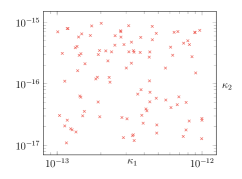
Figure 4.1: Permeabilities’ distribution used for the offline stage

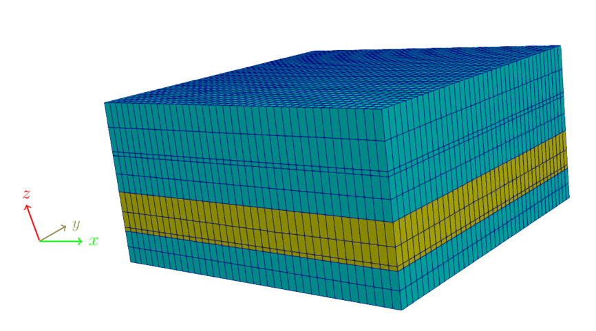
(a) 3D domain

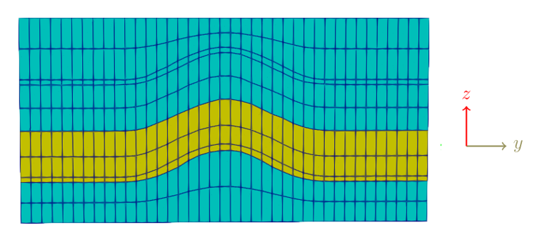
(b) 2D slice

Figure 4.2: Spatial repartition of the permeabilities within $\Omega$: the yellow zone includes cells having the high permeability value $\kappa_{1}$ and the low permeability value $\kappa_{2}$ is used in the blue zone.

4.1 Affine decomposition of the scheme coefficients

To construct the reduced model, we start by applying the EIM as discussed in Section 3.5. We plot in Figure 4.3 the evolution of the interpolation error defined as

$$e_{\rm M,\max}^{\infty}=\max_{\xi\in\Xi_{\rm training}}\frac{\left\|\hat{\boldsymbol{v}}(\xi)-\mathcal{I}_{\rm M}[\hat{\boldsymbol{v}}(\xi)]\right\|_{L^{\infty}}}{\|\hat{\boldsymbol{v}}(\xi)\|_{L^{\infty}}},$$ (4.1)

with respect to the number of parameters $\rm M$. The final number of selected parameters is $\rm M_{EIM}=10$.

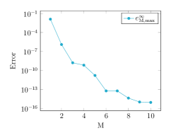
Figure 4.3: Evolution of the EIM interpolation error (4.1) with respect to the number of selected parameters $\rm M$.

To evaluate the accuracy of the linearization with $\rm M_{EIM}=10$, we compute the maximum relative error for new values of $\xi\in\Xi_{\rm test}$. On this sampling, we obtained

$$\max_{\xi\in\Xi_{\rm test}}\frac{\left\|\hat{\boldsymbol{v}}(\xi)-\mathcal{I}_{\rm M_{EIM}}[\hat{\boldsymbol{v}}(\xi)]\right\|_{L^{\infty}}}{\|\hat{\boldsymbol{v}}(\xi)\|_{L^{\infty}}}=4.25\cdot 10^{-16}.$$

4.2 Bounds on the coercivity constants

We consider the successive constraint method to compute a lower bound for the coercivity constant $\alpha_{\boldsymbol{A}_{\rm sym}}$ defined in (3.7). We use the same training set $\Xi_{\rm training}$ and the affine decomposition obtained with the EIM. For this test, we have used $\rm M_{1}=M_{2}=5$ and $\rm tol=1e-04$ (see Appendix B). Since $\rm{M_{EIM}}=10$, we have to solve 10 eigenvalue problems to define $\boldsymbol{\mathcal{B}}$. The offline greedy algorithm 9 generates a parameter set $\Xi_{\rm M}$ of dimension $\rm M=20$. Again to check the quality of the SCM result in the online stage, we compute lower and upper bounds for $\alpha_{\boldsymbol{A}_{\rm sym}}$ for both samplings. More precisely, we compute the values of the ratio

$$r_{\boldsymbol{A}_{\rm sym}}(\xi)=\frac{\alpha_{\boldsymbol{A}_{\rm sym}}(\xi)-\alpha_{\boldsymbol{A}_{\rm sym},\rm LB}(\xi)}{\alpha_{\boldsymbol{A}_{\rm sym},\rm UB}(\xi)-\alpha_{\boldsymbol{A}_{\rm sym},\rm LB}(\xi)},$$

and observe that $r_{\boldsymbol{A}_{\rm sym}}$ is in the range $[0.999,1.00479]$ for all $\xi$ belonging to $\Xi_{\rm training}$ and $\Xi_{\rm test}$.

4.3 POD-Greedy algorithm

As a first test, we construct the reduced model obtained with a POD-Greedy algorithm and the a posteriori estimator $\Delta_{\rm{pr}}^{N}$. We define the following errors

$$\boldsymbol{e}_{\rm{pr,\max}}^{N}=\max_{\xi\in\Xi}{\left|\kern-1.07639pt\left|\kern-1.07639pt\left|\boldsymbol{e}^{N}\right|\kern-1.07639pt\right|\kern-1.07639pt\right|}_{\rm pr},\qquad\Delta_{\rm{pr,\max}}^{N}=\max_{\xi\in\Xi}\;\Delta_{\rm{pr}}^{N},\qquad\eta_{\rm{pr,max}}^{N}=\max_{\xi\in\Xi}\;\frac{\Delta_{\rm{pr}}^{N}}{{\left|\kern-1.07639pt\left|\kern-1.07639pt\left|\boldsymbol{e}^{N}\right|\kern-1.07639pt\right|\kern-1.07639pt\right|}_{\rm pr}},$$

where $\boldsymbol{e}^{N}$ and $\Delta_{\rm{pr}}^{N}$ are given by (3.4) and (3.10) respectively. Figure 4.4 shows the evolution of the a posteriori error estimator $\Delta_{\rm{pr,\max}}^{N}$ along with the true error $\boldsymbol{e}_{\rm{pr,\max}}^{N}$ with respect to the basis dimension $\mathsf{N}_{\rm pr}$. In Figure 4(a), the training parameter set $\Xi_{\rm training}$ is used to evaluate these error indicators, while $\Xi_{\rm test}$ is used in Figure 4(b) following the same sequence of introduction of basis vectors as in POD-Greedy process. The results confirm that the proposed estimator is reliable as it forms an upper bound of the true error in both cases. In the offline phase, the POD-Greedy algorithm generates a basis of dimension $N_{\rm pr}=92$, for which the maximum relative error defined as

$$E_{\rm{pr,\max}}^{N}=\max_{\xi\in\Xi}\;\frac{{\left|\kern-1.07639pt\left|\kern-1.07639pt\left|\boldsymbol{e}^{N}\right|\kern-1.07639pt\right|\kern-1.07639pt\right|}_{\rm pr}}{{\left|\kern-1.07639pt\left|\kern-1.07639pt\left|\boldsymbol{p}_{\mathcal{M}}^{N}\right|\kern-1.07639pt\right|\kern-1.07639pt\right|}_{\rm pr}},$$

reaches $4\cdot 10^{-10}$. To analyse the efficiency of the estimator, we detail in Table 1 the value of the effectivities $\eta_{\rm{pr,max}}^{N}$ in the offline stage for different basis dimensions. We can see that the effectivities are quite good $\mathcal{O}(3)$ and the estimator can be safely used to replace the true error.

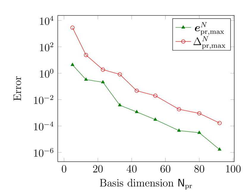
(a) Offline phase

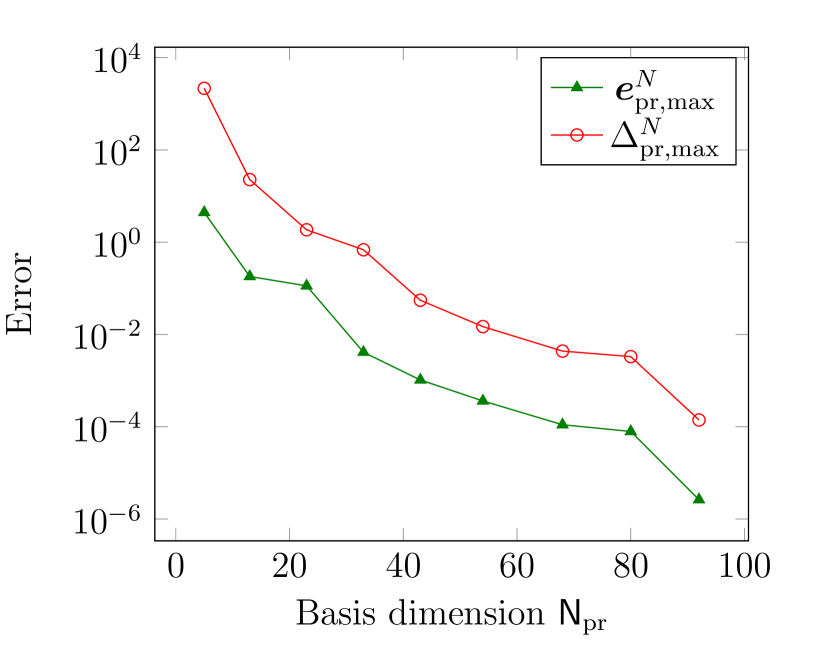
(b) Online phase

Figure 4.4: Maximum true and estimated errors as functions of the basis dimension for the primal problem using the parameter samplings $\Xi_{\rm training}$ on the left and $\Xi_{\rm test}$ on the right.

$\mathsf{N}_{\rm pr}$	$E_{\rm{pr,\max}}^{N}$	$\eta_{\rm{pr,max}}^{N}$
5	1.04e-03	658.1
13	7.94e-05	1061.3
23	5.05e-05	2327.8
33	9.12e-07	1549.5
43	2.81e-07	1400.9
54	7.39e-08	1376.7
68	1.08e-08	677.4
80	7.46e-09	447.1
92	4e-10	392

Table 1: Effectivities of the primal a posteriori error estimate with respect to the basis dimension $\mathsf{N}_{\rm pr}$ in the offline stage.

In addition, we compare in Figure 4.5, the evolution of $\boldsymbol{e}_{\rm{pr,\max}}^{N}$ with respect to the basis dimension $\mathsf{N}_{\rm pr}$ using a POD-Greedy algorithm driven by different choices of the a posteriori error estimator, which are the ones presented in [21] and defined as

$$\bar{\Delta}_{\rm pr,1,max}=\Big{(}\sum_{n=1}^{N}\frac{\Delta t}{\alpha_{\boldsymbol{A}_{\rm sym}}}\|\boldsymbol{r}^{n}\|_{-1}^{2}\Big{)}^{1/2},\quad\text{for}\;\;\boldsymbol{G}^{*}=\boldsymbol{A}^{*},$$ (4.2)

and

$$\bar{\Delta}_{\rm pr,2,max}=\Big{(}\sum_{n=1}^{N}\frac{\Delta t}{\alpha_{\boldsymbol{A}_{\rm sym}}}\|\boldsymbol{r}^{n}\|_{-1}^{2}\Big{)}^{1/2},\quad\text{for}\;\;\boldsymbol{G}^{*}=\boldsymbol{M}+\Delta t\boldsymbol{A}^{*}.$$ (4.3)

For $\mathsf{N}_{\rm pr}<60$, $\boldsymbol{e}_{\rm{pr,\max}}^{N}$ behaves in the same way as for the three choices. For $\mathsf{N}_{\rm pr}>60$, a slight difference appears between the three curves. This trend occurs for both $\Xi_{\rm training}$ and $\Xi_{\rm test}$.

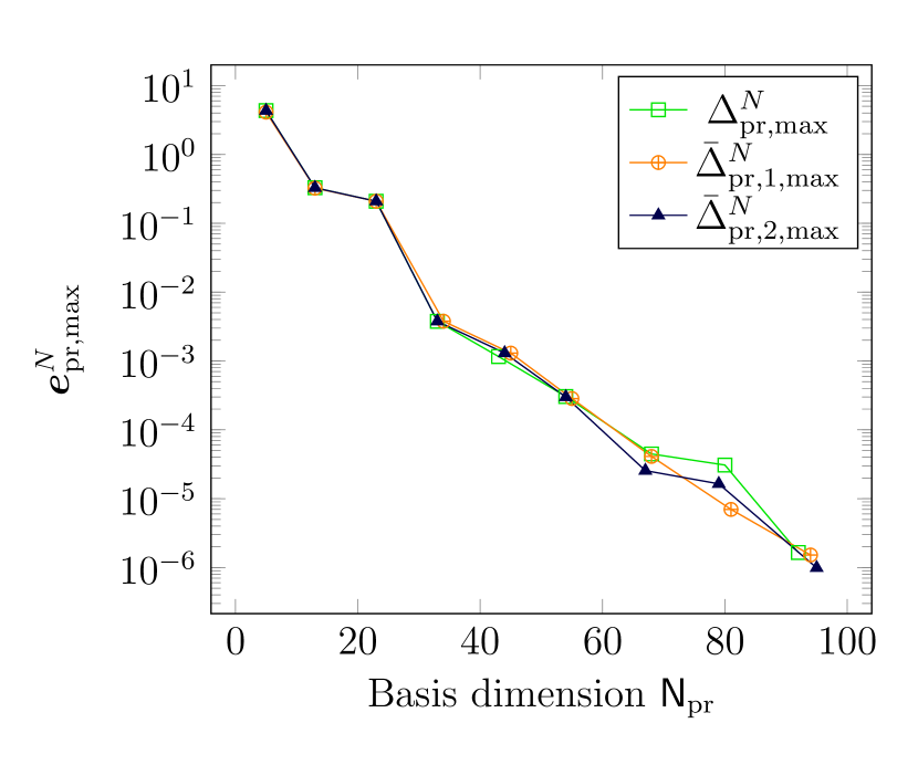
(a) Offline phase

(b) Online phase

Figure 4.5: Maximum true error as a function of the primal basis dimension using $\Xi_{\rm training}$ on the left and $\Xi_{\rm test}$ on the right for a POD-Greedy algorithm driven by (3.10), (4.2) and (4.3).

Next, we build a reduced output by first considering the choice (3.21). We use a POD-Greedy algorithm detailed in Algorithm 21 along with the a posteriori error estimator (3.22). We compare, in that case, the evolution of $\boldsymbol{e}_{\rm{s,\max}}^{N}$ and $\Delta_{\rm{s,\max}}^{N}$ defined as

$$\boldsymbol{e}_{\rm{s}}^{N}=|s^{N}-s^{\mathsf{N}_{\rm s},N}|,\qquad\boldsymbol{e}_{\rm{s,\max}}^{N}=\max_{\xi\in\Xi}|s^{N}-s^{\mathsf{N}_{\rm s},N}|,\qquad\Delta_{\rm{s,\max}}^{N}=\max_{\xi\in\Xi}\;\Delta_{\rm{s}}^{N},$$

with respect to the primal basis dimension $\mathsf{N}_{\rm pr}$ using $\Xi_{\rm training}$ and $\Xi_{\rm test}$. The results are given in Figure 4.6. We notice that, although the reliability of the estimator is verified, $\Delta_{\rm{s}}^{N}$ is not efficient and the effectivities

$$\eta_{\rm{s,max}}^{N}=\max_{\xi\in\Xi}\;\frac{\Delta_{\rm{s}}^{N}}{{\boldsymbol{e}}_{\rm s}^{N}}$$

are quite large as shown in Table 2.

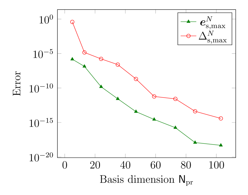
(a) Offline phase

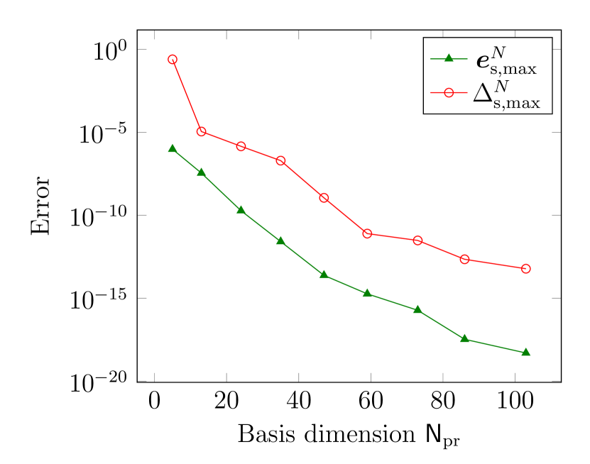
(b) Online phase

Figure 4.6: Maximum true and estimated errors for the first choice of the reduced output as functions of the primal basis dimension using the parameter samplings $\Xi_{\rm training}$ on the left and $\Xi_{\rm test}$ on the right.

$\mathsf{N}_{\rm pr}$	$\mathsf{N}_{\rm du}$	$\eta_{\rm{s,max}}^{N}$
5	10	2.11e+06
13	19	8.08e+06
24	32	9.83e+06
35	44	1.27e+08
47	56	7.21e+06
59	69	4.95e+06
73	84	1.47e+08
86	98	2.72e+08
103	114	1.08e+08

Table 2: Effectivities obtained with the posteriori error estimator (3.22) with respect to the primal and dual basis dimensions $\mathsf{N_{\rm pr}}$ and $\mathsf{N_{\rm du}}$ in the offline stage.

We also observe that $\eta_{\rm{s,max}}^{N}$ becomes less efficient as the final simulation time is increased from $T=10$ days to $T=100$ days (see Figure 4.7).

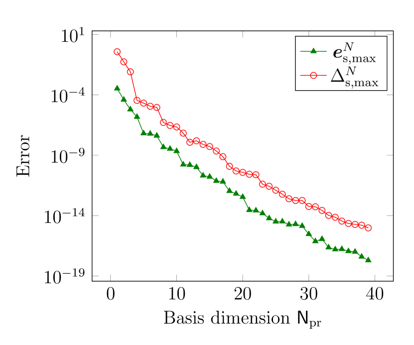
(a) $T=10$ days

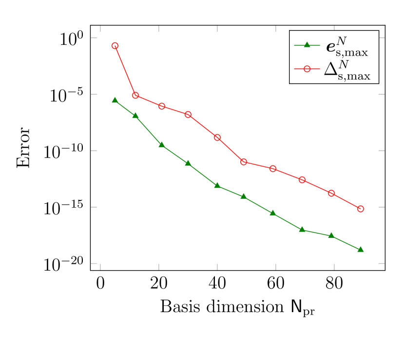
(b) $T=100$ days

Figure 4.7: Maximum true and estimated errors for the first choice of the reduced output as functions of the primal basis dimension with $T=10$ days (on the left) and $T=100$ days (on the right).

We also consider the output estimator presented in [18] as

$$\bar{\Delta}_{\rm s,1,max}=\Big{(}\sum_{n=1}^{N}\frac{\Delta t}{\alpha_{\boldsymbol{A}_{\rm sym}}}\|\boldsymbol{r}^{n}\|_{-1}^{2}\sum_{n=1}^{N}\frac{\Delta t}{\alpha_{\boldsymbol{A}_{\rm sym}}}\|\boldsymbol{\varrho}^{n}\|_{-1}^{2}\Big{)}^{1/2},\quad\text{for}\;\;\boldsymbol{G}^{*}=\boldsymbol{A}^{*},$$ (4.4)

and

$$\bar{\Delta}_{\rm s,2,max}=\Big{(}\sum_{n=1}^{N}\frac{\Delta t}{\alpha_{\boldsymbol{A}_{\rm sym}}}\|\boldsymbol{r}^{n}\|_{-1}^{2}\sum_{n=1}^{N}\frac{\Delta t}{\alpha_{\boldsymbol{A}_{\rm sym}}}\|\boldsymbol{\varrho}^{n}\|_{-1}^{2}\Big{)}^{1/2},\quad\text{for}\;\;\boldsymbol{G}^{*}=\boldsymbol{M}+\Delta t\boldsymbol{A}^{*},$$ (4.5)

and compare in Figure 4.8 the evolution of ${\boldsymbol{e}}_{\rm s,\max}^{N}$ as a function of primal basis dimension $\mathsf{N}_{\rm pr}$ using a POD-Greedy algorithm controlled by (3.22), (4.4) and (4.5). We observe that the true error is exactly the same using (3.22) and (4.5).

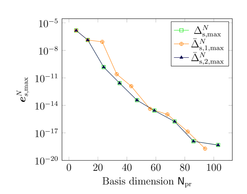
(a) Offline phase

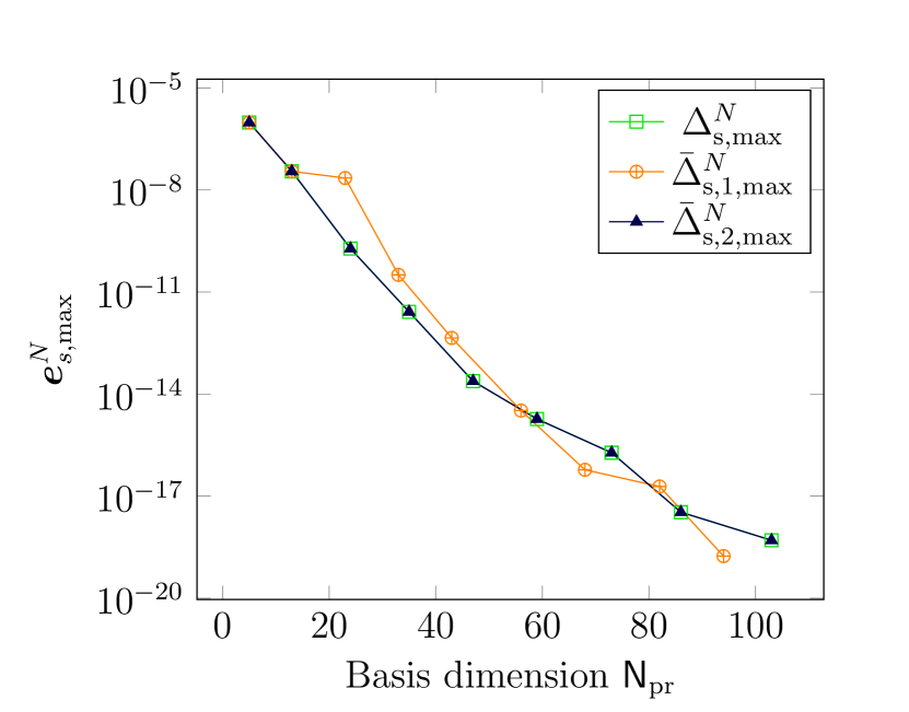
(b) Online phase

Figure 4.8: Estimated errors for the first choice of the reduced output as a function of the primal basis dimension for a POD-Greedy algorithm driven by (3.22), (4.4) and (4.5) using $\Xi_{\rm training}$ on the left and $\Xi_{\rm test}$ on the right.

We now employ the second definition of the output error (3.23) and estimator (3.24) and analyze the evolution of the POD-Greedy algorithm in the offline and online stages. The results are shown in Figure 4.9. We define the following errors

$$\widetilde{\boldsymbol{e}}_{\rm{s}}^{N}=|s^{N}-\widetilde{s}^{\mathsf{N}_{\rm s},N}|,\qquad\widetilde{\boldsymbol{e}}_{\rm{s,\max}}^{N}=\max_{\xi\in\Xi}|s^{N}-\widetilde{s}^{\mathsf{N}_{\rm s},N}|,\qquad\widetilde{\Delta}_{\rm{s,\max}}^{N}=\max_{\xi\in\Xi}\;\widetilde{\Delta}_{\rm{s}}^{N},\qquad\widetilde{\eta}_{\rm{s,max}}^{N}=\max_{\xi\in\Xi}\;\frac{\widetilde{\Delta}_{\rm{s}}^{N}}{\widetilde{\boldsymbol{e}}_{\rm s}^{N}}.$$

Table 3 shows that the proposed estimator is very close to the true error and behaves better in terms of effectivity compared to ${\eta}_{\rm{s,max}}^{N}$: indeed, from $\mathsf{N}_{\rm pr}=59$, $\widetilde{\eta}_{\rm{s,max}}^{N}$ behaves as $\mathcal{O}(1)$. However, we observe that the first choice of the reduced output (3.21) and the corresponding a posteriori error estimate (3.22) provide better results in terms of accuracy and size of the basis dimensions: to obtain a precision of $1e-10$, we need a primal basis of dimension $\mathsf{N}_{\rm pr}=24$ and a dual basis of dimension $\mathsf{N}_{\rm du}=32$ with the first choice while the second choice requires bases whoses sizes are $\mathsf{N}_{\rm pr}=72$ and $\mathsf{N}_{\rm du}=84$. Finally, we introduce the output estimator presented in [18] as

$$\bar{\bar{\Delta}}_{\rm s,1,max}=\Big{(}\sum_{n=1}^{N}\frac{\Delta t}{\alpha_{\boldsymbol{A}_{\rm sym}}}\|\boldsymbol{r}^{n}\|_{-1}^{2}\sum_{n=1}^{N}\frac{\Delta t}{\alpha_{\boldsymbol{A}_{\rm sym}}}\|\boldsymbol{\varrho}^{n}\|_{-1}^{2}\Big{)}^{1/2}+\Delta t\;\sum_{n=0}^{N-1}\big{|}\big{\langle}{\boldsymbol{r}}^{n+1},\boldsymbol{\Psi}^{\mathsf{N}_{\rm du},n}\big{\rangle}\big{|},\quad\text{for}\;\;\boldsymbol{G}^{*}=\boldsymbol{A}^{*},$$ (4.6)

and

$$\bar{\bar{\Delta}}_{\rm s,2,max}=\Big{(}\sum_{n=1}^{N}\frac{\Delta t}{\alpha_{\boldsymbol{A}_{\rm sym}}}\|\boldsymbol{r}^{n}\|_{-1}^{2}\sum_{n=1}^{N}\frac{\Delta t}{\alpha_{\boldsymbol{A}_{\rm sym}}}\|\boldsymbol{\varrho}^{n}\|_{-1}^{2}\Big{)}^{1/2}+\Delta t\;\sum_{n=0}^{N-1}\big{|}\big{\langle}{\boldsymbol{r}}^{n+1},\boldsymbol{\Psi}^{\mathsf{N}_{\rm du},n}\big{\rangle}\big{|},\quad\text{for}\;\;\boldsymbol{G}^{*}=\boldsymbol{M}+\Delta t\boldsymbol{A}^{*},$$ (4.7)

and compare, in Figure 4.10, the evolution of $\widetilde{\boldsymbol{e}}_{\rm{s,\max}}^{N}$ using a POD-Greedy algorithm controlled by (3.24), (4.6) and (4.7). We observe that the accuracy is the same when employing the estimators (3.24) and (4.7) and that the curve related to (4.6) lies above the other curves for $\mathsf{N}_{\rm pr}<70$ and below them for $\mathsf{N}_{\rm pr}>70$.

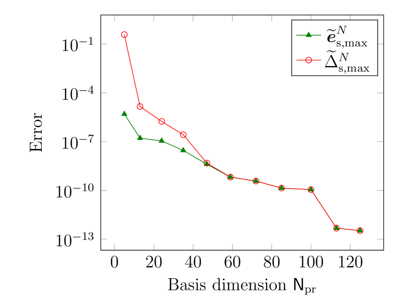
(a) Offline phase

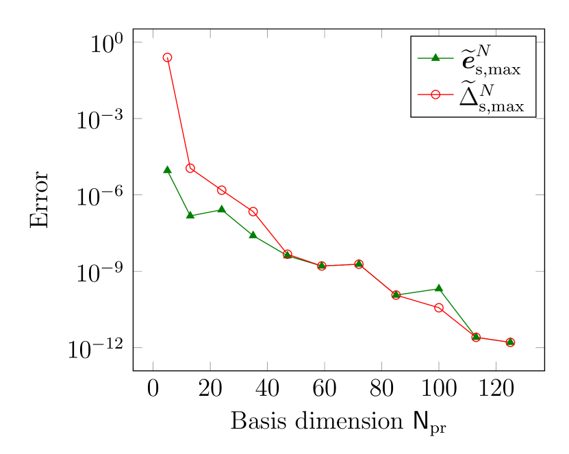
(b) Online phase

Figure 4.9: Maximum true and estimated errors for the second choice of the reduced output as functions of the primal basis dimension using $\Xi_{\rm training}$ on the left and $\Xi_{\rm test}$ on the right.

$\mathsf{N}_{\rm pr}$	$\mathsf{N}_{\rm du}$	$\widetilde{\eta}_{\rm{s,max}}^{N}$
5	10	103103
13	19	222673
24	32	2066.3
35	44	23.6
47	56	1266.5
59	69	1.26
72	84	1.06
85	99	1.34
100	115	1.18
113	129	1.0
125	143	1.01

Table 3: Effectivities for the a posteriori error estimator (3.24) with respect to the primal and dual basis dimensions $\mathsf{N_{\rm pr}}$ and $\mathsf{N_{\rm du}}$ in the offline stage.

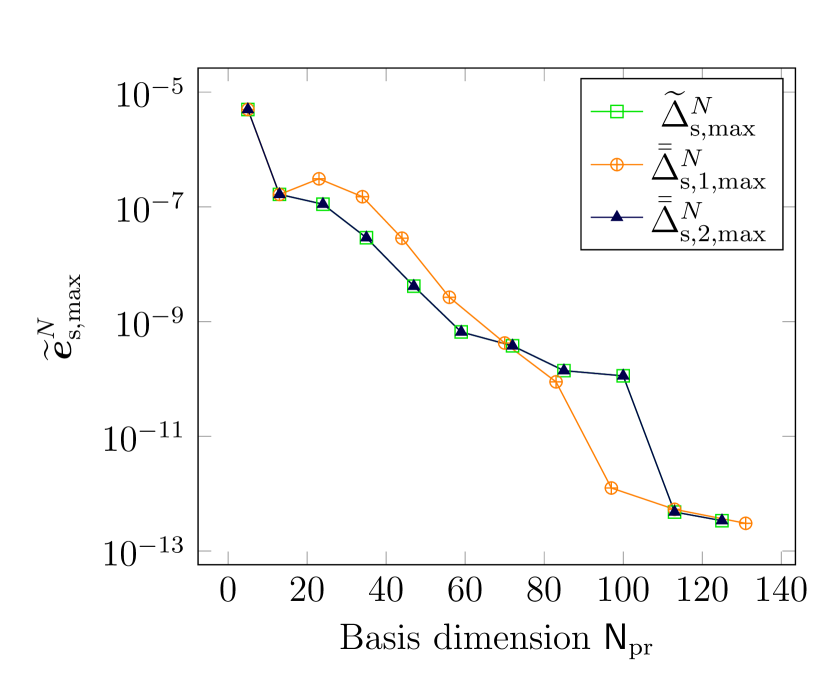
(a) Offline phase

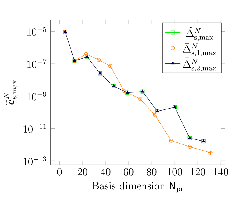
(b) Online phase

Figure 4.10: Estimated errors for the second choice of the reduced output as a function of the primal basis dimension for a POD-Greedy algorithm driven by (3.24), (4.6) and (4.7) using $\Xi_{\rm training}$ on the left and $\Xi_{\rm test}$ on the right.

4.4 Computational time effort

Here we give an indication of the time spent at each stage of the construction and evaluation of the reduced model.

Offline stage.

We plot in Figure 4.11 the evolution of the computation times related to the different stages of the reduced-basis construction as functions of the primal basis dimension $\mathsf{N}_{\rm pr}$. The time is calculated as a factor of the time $u$ required to run one single high-fidelity simulation. Concerning the EIM and SCM algorithms, these two procedures are applied once at the beginning of the offline stage before starting the POD-Greedy process. This explains why their cumulated times appear as constant in the plot. These times amount to $100\times u$ seconds and $39\times u$ seconds respectively. The cumulated time spent in the Greedy process is represented in blue up to $\mathsf{N}_{\rm pr}=103$. For each greedy iteration, the given values include the times required to assemble and compute the reduced solutions (3.2) and (3.16) and the residuals (3.27)–(3.30) for all parameters of the sampling. These operations depend on the sizes $\mathsf{N}_{\rm pr}$ and $\mathsf{N}_{\rm du}$ and therefore increase as the Greedy process evolves. The "Greedy" time therefore includes the time spent in assembling the reduced primal and dual systems (3.3) and (3.17) for all parameters of the sampling. This time is represented under the label "LF assembly" too. It is quite significant in the offline stage since all products involving the terms of the affine decompositions with the new bases matrices should be updated. This cost is of course substantially reduced in the online stage once the bases are fixed. The cumulated calculation time of the POD method is represented in Figure 4.11. It is linear with respect to $\mathsf{N}_{\rm pr}$. It includes the times required to run the high-fidelity simulations and the extractions of the POD modes. In both cases, for each selected parameter, these times are roughly constant.

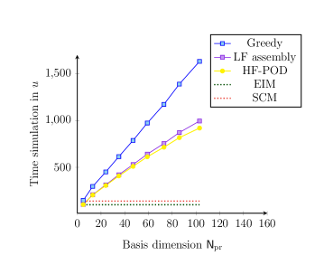
Figure 4.11: Offline time computation effort.

Online stage.

Given a new parameter value $\xi\in\Xi_{\rm test}$, with our implementation, the time used in the online stage to compute $\boldsymbol{p}^{\mathsf{N}_{\rm pr},N}$ and its corresponding reduced output at $T=200$ days and with $\mathsf{N}_{\rm pr}=92$ is divided by a factor of $10$ compared to one HF run needed to obtain $\boldsymbol{p}_{\mathcal{M}}^{N}$. The high-fidelity model (2.1) is solved using a stabilized bi-conjugate gradient method with an incomplete LU preconditioner, where the tolerance is set to $10^{-14}$. The reduced model (3.3) is directly solved using an LU-Decomposition.

5 Conclusion

In this work, we have discussed a reduced basis method for (finite volume approximations of) parabolic PDEs. We have introduced a new rigorous a posteriori estimator to evaluate the reduction error in a new discrete space-time energy norm independently of the parameter. We have performed numerical simulations in the context of porous media flows (single-phase flows of slightly compressible fluid parametrized by the permeability) to assess the reliability of the a posteriori error bound and its efficiency at selecting a reduced basis within a POD-Greedy algorithm.

Our numerical results show that our new approach can efficiently reduce the computational cost of engineering studies with many parameter values in the context of porous media flows, especially on choosing well the reduced output in goal-oriented cases with linear QOIs. The discussed methodology can be also considered to estimate different types of linear quantity of interests such as the pressure variation along faults far from the well injection area. Indeed, understanding how injection activities affect pressure distribution in fault networks helps in mitigating risks associated with CO2 migration, fault activation, and potential leakage into overlying aquifers.

Appendix A Proofs of various propositions

A.1 Proof of Proposition 3.1

Proof.

For each $\boldsymbol{v}\in\mathbb{R}^{\mathcal{N}}$, we have

$$\begin{split}\left\langle(\boldsymbol{M}+\Delta t\boldsymbol{A})\boldsymbol{e}^{n},\boldsymbol{v}\right\rangle&=\left\langle\boldsymbol{M}\boldsymbol{e}^{n-1},\boldsymbol{v}\right\rangle-\Delta t\,\langle\boldsymbol{r}^{n},\boldsymbol{v}\rangle.\end{split}$$ (A.1)

We apply $\boldsymbol{e}^{n}$ to (A.1). We apply Cauchy-Schwarz inequality and use (3.6). This leads to

$$\left\langle(\boldsymbol{M}+\Delta t\boldsymbol{A})\boldsymbol{e}^{n},\boldsymbol{e}^{n}\right\rangle\leq\|\boldsymbol{M}^{1/2}\boldsymbol{e}^{n-1}\|\|\boldsymbol{M}^{1/2}\boldsymbol{e}^{n}\|+\Delta t\;\|\boldsymbol{r}^{n}\|_{-1}\|\boldsymbol{e}^{n}\|_{\boldsymbol{G}^{*}}.$$ (A.2)

Now, recalling Young’s inequality (for $c\in\mathbb{R}$, $d\in\mathbb{R}$, $\rho\in\mathbb{R}_{+}$):

$$2|c|\,|d|\leq\frac{1}{\rho^{2}}c^{2}+\rho^{2}d^{2},$$ (A.3)

and apply it twice: once for $c=\|\boldsymbol{M}^{1/2}\boldsymbol{e}^{n-1}\|$, $d=\|\boldsymbol{M}^{1/2}\boldsymbol{e}^{n}\|$ and $\rho=1$ to get

$$2\|\boldsymbol{M}^{1/2}\boldsymbol{e}^{n-1}\|\,\|\boldsymbol{M}^{1/2}\boldsymbol{e}^{n}\|\leq\langle\boldsymbol{M}\boldsymbol{e}^{n-1},\boldsymbol{e}^{n-1}\rangle+\langle\boldsymbol{M}\boldsymbol{e}^{n},\boldsymbol{e}^{n}\rangle$$ (A.4)

and another time for $c=\|\boldsymbol{r}^{n}\|_{-1}$, $d=\|\boldsymbol{e}^{n}\|_{\boldsymbol{G}^{*}}$ and $\rho=\sqrt{\alpha_{\boldsymbol{A}_{\rm sym}}}$ to obtain

$$2\|\boldsymbol{r}^{n}\|_{-1}\|\boldsymbol{e}^{n}\|_{\boldsymbol{G}^{*}}\leq\frac{1}{\alpha_{\boldsymbol{A}_{\rm sym}}}\;\|\boldsymbol{r}^{n}\|_{-1}^{2}+\alpha_{\boldsymbol{A}_{\rm sym}}\;\|\boldsymbol{e}^{n}\|_{\boldsymbol{G}^{*}}^{2}.$$ (A.5)

Now the definition of the coercivity constant (3.7) leads to

$$2\|\boldsymbol{r}^{n}\|_{-1}\;\|\boldsymbol{e}^{n}\|_{\boldsymbol{G}^{*}}\leq\frac{1}{\alpha_{\boldsymbol{A}_{\rm sym}}}\;\|\boldsymbol{r}^{n}\|_{-1}^{2}+\langle\boldsymbol{A}_{\rm sym}\;\boldsymbol{e}^{n},\boldsymbol{e}^{n}\rangle.$$ (A.6)

Combining (A.2), (A.4) and (A.6) yields

$$\begin{split}\langle\boldsymbol{M}\boldsymbol{e}^{n},\boldsymbol{e}^{n}\rangle+\Delta t\;\langle\boldsymbol{A}\boldsymbol{e}^{n},\boldsymbol{e}^{n}\rangle&\leq\frac{1}{2}\langle\boldsymbol{M}\boldsymbol{e}^{n-1},\boldsymbol{e}^{n-1}\rangle+\frac{1}{2}\langle\boldsymbol{M}\boldsymbol{e}^{n},\boldsymbol{e}^{n}\rangle\\ &+\frac{\Delta t}{2}\langle\boldsymbol{A}_{\rm sym}\;\boldsymbol{e}^{n},\boldsymbol{e}^{n}\rangle+\frac{\Delta t}{2\alpha_{\boldsymbol{A}_{\rm sym}}}\;\|\boldsymbol{r}^{n}\|_{-1}^{2}.\end{split}$$ (A.7)

Since $\langle\boldsymbol{A}_{\rm skew}\;\boldsymbol{e}^{n},\boldsymbol{e}^{n}\rangle=0$ and $\langle\boldsymbol{A}_{\rm sym}\;\boldsymbol{e}^{n},\boldsymbol{e}^{n}\rangle=\langle\boldsymbol{A}\boldsymbol{e}^{n},\boldsymbol{e}^{n}\rangle$, we obtain

$$\langle\boldsymbol{M}\boldsymbol{e}^{n},\boldsymbol{e}^{n}\rangle-\langle\boldsymbol{M}\boldsymbol{e}^{n-1},\boldsymbol{e}^{n-1}\rangle+\Delta t\;\langle\boldsymbol{A}_{\rm sym}\;\boldsymbol{e}^{n},\boldsymbol{e}^{n}\rangle\leq\frac{\Delta t}{\alpha_{\boldsymbol{A}_{\rm sym}}}\|\boldsymbol{r}^{n}\|_{-1}^{2}.$$ (A.8)

Finally, we sum (A.8) over $\{1,\ldots,n\}$ and consider that $\boldsymbol{e}^{0}=0$ to get

$$\langle\boldsymbol{M}\boldsymbol{e}^{n},\boldsymbol{e}^{n}\rangle+\sum_{m=1}^{n}\Delta t\;\langle\boldsymbol{A}_{\rm sym}\;\boldsymbol{e}^{m},\boldsymbol{e}^{m}\rangle\leq\sum_{m=1}^{n}\frac{\Delta t}{\alpha_{\boldsymbol{A}_{\rm sym}}}\|\boldsymbol{r}^{m}\|_{-1}^{2}.$$ (A.9)

From (A.9), we have

$$\begin{split}\sum_{n=1}^{N}\langle\boldsymbol{M}\boldsymbol{e}^{n},\boldsymbol{e}^{n}\rangle\leq\frac{\Delta t}{\alpha_{\boldsymbol{A}_{\rm sym}}}\sum_{n=1}^{N}(N+1-n)\|\boldsymbol{r}^{n}\|_{-1}^{2}\leq\frac{T}{\alpha_{\boldsymbol{A}_{\rm sym}}}\sum_{n=1}^{N}\|\boldsymbol{r}^{n}\|_{-1}^{2}.\end{split}$$ (A.10)

As a consequence,

$$\sum_{n=1}^{N}\langle\boldsymbol{M}\boldsymbol{e}^{n},\boldsymbol{e}^{n}\rangle\leq\frac{T}{\alpha_{\boldsymbol{A}_{\rm sym}}}\sum_{n=1}^{N}\|\boldsymbol{r}^{n}\|_{-1}^{2}.$$ (A.11)

On the other hand, using (A.9), we can write

$$\sum_{m=1}^{n}\langle\boldsymbol{A}_{\rm sym}\boldsymbol{e}^{m},\boldsymbol{e}^{m}\rangle\leq\frac{1}{\alpha_{\boldsymbol{A}_{\rm sym}}}\sum_{m=1}^{n}\|\boldsymbol{r}^{m}\|_{-1}^{2},\quad\forall n\in\{1,\ldots,N\}.$$ (A.12)

Now (A.11) with (A.12) for $n=N$ enable the following inequality

$$\sum_{m=1}^{N}\big{[}\langle\boldsymbol{M}\boldsymbol{e}^{m},\boldsymbol{e}^{m}\rangle+\Delta t\;\langle\boldsymbol{A}_{\rm sym}\;\boldsymbol{e}^{m},\boldsymbol{e}^{m}\rangle\big{]}\leq\frac{T+\Delta t}{\alpha_{\boldsymbol{A}_{\rm sym}}}\sum_{m=1}^{N}\|\boldsymbol{r}^{m}\|_{-1}^{2}$$ (A.13)

where it is possible to use (3.8) and write

$$\begin{split}\alpha_{\boldsymbol{G},\rm LB}\;\sum_{m=1}^{N}\big{[}\langle\boldsymbol{M}\boldsymbol{e}^{m},\boldsymbol{e}^{m}\rangle+\Delta t\;\langle\boldsymbol{A}_{\rm sym}^{*}\;\boldsymbol{e}^{m},\boldsymbol{e}^{m}\rangle\big{]}&\leq\sum_{m=1}^{N}[\langle\boldsymbol{M}\boldsymbol{e}^{m},\boldsymbol{e}^{m}\rangle+\Delta t\;\langle\boldsymbol{A}_{\rm sym}\;\boldsymbol{e}^{m},\boldsymbol{e}^{m}\rangle]\\ &\leq\frac{T+\Delta t}{\alpha_{\boldsymbol{A}_{\rm sym}}}\sum_{m=1}^{N}\|\boldsymbol{r}^{m}\|_{-1}^{2}\\ &\leq\frac{T+\Delta t}{\alpha_{\boldsymbol{A}_{\rm sym,\rm LB}}}\sum_{m=1}^{N}\|\boldsymbol{r}^{m}\|_{-1}^{2}\end{split}$$ (A.14)

i.e. an upper bound of the error that is independent of the parameter $\xi$ as opposed to [21, Prop. 4.3]. ∎

A.2 Proof of Proposition 3.2

Proof.

We start by writing

$$\big{\langle}(\boldsymbol{M}+\Delta t\boldsymbol{A}^{T})\boldsymbol{\varepsilon}^{m},\boldsymbol{v}\big{\rangle}=\left\langle\boldsymbol{M}\boldsymbol{\varepsilon}^{m+1},\boldsymbol{v}\right\rangle-\Delta t\,\big{\langle}\boldsymbol{\varrho}^{m},\boldsymbol{v}\big{\rangle},\quad\forall\boldsymbol{v}\in\mathbb{R}^{\mathcal{N}},$$

and then take $\boldsymbol{v}=\boldsymbol{\varepsilon}^{m}$ to obtain

$$\big{\langle}(\boldsymbol{M}+\Delta t\boldsymbol{A}^{T})\boldsymbol{\varepsilon}^{m},\boldsymbol{\varepsilon}^{m}\big{\rangle}=\langle\boldsymbol{M}\boldsymbol{\varepsilon}^{m+1},\boldsymbol{\varepsilon}^{m}\rangle-\Delta t\,\big{\langle}\boldsymbol{\varrho}^{m},\boldsymbol{\varepsilon}^{m}\big{\rangle}.$$

We apply Cauchy-Schwarz inequality and use (3.19)

$$\big{\langle}(\boldsymbol{M}+\Delta t\boldsymbol{A}^{T})\boldsymbol{\varepsilon}^{m},\boldsymbol{\varepsilon}^{m}\big{\rangle}\leq\|\boldsymbol{M}^{1/2}\boldsymbol{\varepsilon}^{m+1}\|\|\boldsymbol{M}^{1/2}\boldsymbol{\varepsilon}^{m}\|+\Delta t\,\|\boldsymbol{\varrho}^{m}\|_{-1}\;\|\boldsymbol{\varepsilon}^{m}\|_{\boldsymbol{G}^{*}}.$$ (A.15)

Similarly to the primal problem, we apply inequality (A.3) twice and get

$$2\|\boldsymbol{M}^{1/2}\boldsymbol{\varepsilon}^{m+1}\|\|\boldsymbol{M}^{1/2}\boldsymbol{\varepsilon}^{m}\| \leq\left\langle\boldsymbol{M}\boldsymbol{\varepsilon}^{m+1},\boldsymbol{\varepsilon}^{m+1}\right\rangle+\left\langle\boldsymbol{M}\boldsymbol{\varepsilon}^{m},\boldsymbol{\varepsilon}^{m}\right\rangle,$$ (A.16)

$$2\|\boldsymbol{\varrho}^{m}\|_{-1}\|\boldsymbol{\varepsilon}^{m}\|_{\boldsymbol{G}^{*}} \leq\frac{1}{\alpha_{\boldsymbol{A}_{\rm sym}}}\|\boldsymbol{\varrho}^{m}\|_{-1}^{2}+\alpha_{\boldsymbol{A}_{\rm sym}}\|\boldsymbol{\varepsilon}^{m}\|_{\boldsymbol{G}^{*}}^{2}.$$ (A.17)

Based on the definition of $\alpha_{\boldsymbol{A}_{\rm sym}}$, (A.17) becomes

$$\begin{split}2\|\boldsymbol{\varrho}^{m}\|_{-1}\|\boldsymbol{\varepsilon}^{m}\|_{\boldsymbol{G}^{*}}&\leq\frac{1}{\alpha_{\boldsymbol{A}_{\rm sym}}}\|\boldsymbol{\varrho}^{m}\|_{-1}^{2}+\big{\langle}\boldsymbol{A}_{\rm sym}\;\boldsymbol{\varepsilon}^{m},\boldsymbol{\varepsilon}^{m}\big{\rangle}\\ &=\frac{1}{\alpha_{\boldsymbol{A}_{\rm sym}}}\|\boldsymbol{\varrho}^{m}\|_{-1}^{2}+\big{\langle}\boldsymbol{A}\boldsymbol{\varepsilon}^{m},\boldsymbol{\varepsilon}^{m}\big{\rangle},\quad\text{since}\;\big{\langle}\boldsymbol{A}_{\rm skew}\;\boldsymbol{\varepsilon}^{m},\boldsymbol{\varepsilon}^{m}\big{\rangle}=0\\ &=\frac{1}{\alpha_{\boldsymbol{A}_{\rm sym}}}\|\boldsymbol{\varrho}^{m}\|_{-1}^{2}+\big{\langle}\boldsymbol{\varepsilon}^{m},\boldsymbol{A}^{T}\boldsymbol{\varepsilon}^{m}\big{\rangle}\\ &=\frac{1}{\alpha_{\boldsymbol{A}_{\rm sym}}}\|\boldsymbol{\varrho}^{m}\|_{-1}^{2}+\big{\langle}\boldsymbol{A}^{T}\boldsymbol{\varepsilon}^{m},\boldsymbol{\varepsilon}^{m}\big{\rangle}.\end{split}$$ (A.18)

Now, inequalities (A.15)–(A.18) lead to

$$\big{\langle}\boldsymbol{M}\boldsymbol{\varepsilon}^{m},\boldsymbol{\varepsilon}^{m}\big{\rangle}-\big{\langle}\boldsymbol{M}\boldsymbol{\varepsilon}^{m+1},\boldsymbol{\varepsilon}^{m+1}\big{\rangle}+\Delta t\,\big{\langle}\boldsymbol{A}^{T}\boldsymbol{\varepsilon}^{m},\boldsymbol{\varepsilon}^{m}\big{\rangle}\leq\frac{\Delta t}{\alpha_{\boldsymbol{A}_{\rm sym}}}\|\boldsymbol{\varrho}^{m}\|_{-1}^{2}.$$ (A.19)

We finally sum (A.19) over $\{n,\ldots,N-1\}$ and suppose that $\boldsymbol{\varepsilon}^{N}=0$. We get

$$\big{\langle}{\boldsymbol{\varepsilon}^{n}},\boldsymbol{M}{\boldsymbol{\varepsilon}}^{n}\big{\rangle}+\Delta t\sum_{m=n}^{N-1}\big{\langle}{\boldsymbol{\varepsilon}}^{m},\boldsymbol{A}^{T}{\boldsymbol{\varepsilon}}^{m}\big{\rangle}\leq\frac{\Delta t}{\alpha_{\boldsymbol{A}_{\rm sym}}}\sum_{m=n}^{N-1}\|\boldsymbol{\varrho}^{m}\|_{-1}^{2}.$$ (A.20)

Inequality (A.20) holds true for all $n\in\{0,\ldots,N-1\}$. So we can write

$$\begin{split}\sum_{n=0}^{N-1}\left\langle{\boldsymbol{\varepsilon}^{n}},\boldsymbol{M}{\boldsymbol{\varepsilon}}^{n}\right\rangle&\leq\frac{\Delta t}{\alpha_{\boldsymbol{A}_{\rm sym}}}\sum_{n=0}^{N-1}\sum_{m=n}^{N-1}\|\boldsymbol{\varrho}^{m}\|_{-1}^{2}\\ &\leq\frac{\Delta t}{\alpha_{\boldsymbol{A}_{\rm sym}}}\sum_{n=0}^{N-1}(n+1)\|\boldsymbol{\varrho}^{n}\|_{-1}^{2}\\ &\leq\frac{N\Delta t}{\alpha_{\boldsymbol{A}_{\rm sym}}}\sum_{n=0}^{N-1}\|\boldsymbol{\varrho}^{n}\|_{-1}^{2}\\ &=\frac{T}{\alpha_{\boldsymbol{A}_{\rm sym}}}\sum_{n=0}^{N-1}\|\boldsymbol{\varrho}^{n}\|_{-1}^{2}.\end{split}$$ (A.21)

Then,

$$\sum_{n=0}^{N-1}\big{\langle}{\boldsymbol{\varepsilon}^{n}},\boldsymbol{M}{\boldsymbol{\varepsilon}}^{n}\big{\rangle}\leq\frac{T}{\alpha_{\boldsymbol{A}_{\rm sym}}}\sum_{n=0}^{N-1}\|\boldsymbol{\varrho}^{n}\|_{-1}^{2}.$$ (A.22)

On the other side, again using (A.20), we have in particular for $n=0$

$$\Delta t\;\sum_{m=0}^{N-1}\big{\langle}{\boldsymbol{\varepsilon}}^{m},\boldsymbol{A}^{T}{\boldsymbol{\varepsilon}}^{m}\big{\rangle}\leq\frac{\Delta t}{\alpha_{\boldsymbol{A}_{\rm sym}}}\sum_{m=0}^{N-1}\|\boldsymbol{\varrho}^{m}\|_{-1}^{2}.$$ (A.23)

Combining (A.22) and (A.23), leads to

$$\sum_{m=0}^{N-1}\big{[}\left\langle{\boldsymbol{\varepsilon}^{m}},\boldsymbol{M}{\boldsymbol{\varepsilon}}^{m}\right\rangle+\Delta t\,\big{\langle}{\boldsymbol{\varepsilon}}^{m},\boldsymbol{A}^{T}{\boldsymbol{\varepsilon}}^{m}\big{\rangle}\big{]}\leq\frac{T+\Delta t}{\alpha_{\boldsymbol{A}_{\rm sym}}}\sum_{m=0}^{N-1}\|\boldsymbol{\varrho}^{m}\|_{-1}^{2}.$$ (A.24)

Now, since

$$\big{\langle}{\boldsymbol{\varepsilon}}^{m},\boldsymbol{A}^{T}{\boldsymbol{\varepsilon}}^{m}\big{\rangle}=\big{\langle}\boldsymbol{A}{\boldsymbol{\varepsilon}}^{m},{\boldsymbol{\varepsilon}}^{m}\big{\rangle}=\big{\langle}\boldsymbol{A}_{\rm sym}\;{\boldsymbol{\varepsilon}}^{m},{\boldsymbol{\varepsilon}}^{m}\big{\rangle},$$

we get

$$\sum_{m=0}^{N-1}\big{[}\big{\langle}{\boldsymbol{\varepsilon}^{m}},\boldsymbol{M}{\boldsymbol{\varepsilon}}^{m}\big{\rangle}+\Delta t\,\big{\langle}{\boldsymbol{\varepsilon}}^{m},\boldsymbol{A}_{\rm sym}\;{\boldsymbol{\varepsilon}}^{m}\big{\rangle}\big{]}\leq\frac{T+\Delta t}{\alpha_{\boldsymbol{A}_{\rm sym}}}\sum_{m=0}^{N-1}\|\boldsymbol{\varrho}^{m}\|_{-1}^{2}.$$ (A.25)

Finally, we recall the definition of $\alpha_{\boldsymbol{G}}$, which results in

$$\sum_{m=0}^{N-1}\big{[}\big{\langle}{\boldsymbol{\varepsilon}^{m}},\boldsymbol{M}{\boldsymbol{\varepsilon}}^{m}\big{\rangle}+\Delta t\,\big{\langle}{\boldsymbol{\varepsilon}}^{m},\boldsymbol{A}_{\rm sym}^{*}\;{\boldsymbol{\varepsilon}}^{m}\big{\rangle}\big{]}\leq\frac{T+\Delta t}{\alpha_{\boldsymbol{G},\rm LB}\alpha_{\boldsymbol{A}_{\rm sym,\rm LB}}}\sum_{m=0}^{N-1}\|\boldsymbol{\varrho}^{m}\|_{-1}^{2}.$$ (A.26)

∎

A.3 Proof of Proposition 3.3

Proof.

From (3.13), we have

$$\big{\langle}\boldsymbol{M}(\boldsymbol{\boldsymbol{\psi}}_{\mathcal{M},n}^{k}-\boldsymbol{\psi}_{\mathcal{M},n}^{k+1})+\Delta t\;\boldsymbol{A}^{T}\boldsymbol{\psi}_{\mathcal{M},n}^{k},\boldsymbol{e}^{k+1}\big{\rangle}=0.$$

We then sum over $k=0,\ldots,n-1$, to obtain

$$\langle\boldsymbol{M}(\boldsymbol{\psi}_{\mathcal{M},n}^{0}-\boldsymbol{\psi}_{\mathcal{M},n}^{1}),\boldsymbol{e}^{1}\rangle+\langle\boldsymbol{M}(\boldsymbol{\psi}_{\mathcal{M},n}^{1}-\boldsymbol{\psi}_{\mathcal{M},n}^{2}),\boldsymbol{e}^{2}\rangle+\ldots+\langle\boldsymbol{M}(\boldsymbol{\psi}_{\mathcal{M},n}^{n-1}-\boldsymbol{\psi}_{\mathcal{M},n}^{n}),\boldsymbol{e}^{n}\rangle+\Delta t\sum_{k=0}^{n-1}\langle\boldsymbol{A}^{T}\boldsymbol{\psi}_{\mathcal{M},n}^{k},\boldsymbol{e}^{k+1}\rangle=0,$$

which gives us

$$\begin{split}\langle\boldsymbol{M}\boldsymbol{\psi}_{\mathcal{M},n}^{0},\boldsymbol{e}^{1}\rangle-&\langle\boldsymbol{M}\boldsymbol{\psi}_{\mathcal{M},n}^{1},\boldsymbol{e}^{1}\rangle+\langle\boldsymbol{M}\boldsymbol{\psi}_{\mathcal{M},n}^{1},\boldsymbol{e}^{2}\rangle-\langle\boldsymbol{M}\boldsymbol{\psi}_{\mathcal{M},n}^{2},\boldsymbol{e}^{2}\rangle+\ldots\\ &+\langle\boldsymbol{M}\boldsymbol{\psi}_{\mathcal{M},n}^{n-1},\boldsymbol{e}^{n}\rangle-\langle\boldsymbol{M}\boldsymbol{\psi}_{\mathcal{M},n}^{n},\boldsymbol{e}_{n}^{n}\rangle+\Delta t\sum_{k=0}^{n-1}\langle\boldsymbol{A}^{T}\boldsymbol{\psi}_{\mathcal{M},n}^{k},\boldsymbol{e}^{k+1}\rangle=0,\end{split}$$

leading to

$$\sum_{k=0}^{n-1}\langle\boldsymbol{M}\boldsymbol{\psi}_{\mathcal{M},n}^{k},\boldsymbol{e}^{k+1}\rangle-\sum_{k=1}^{n-1}\langle\boldsymbol{M}\boldsymbol{\psi}_{\mathcal{M},n}^{k},\boldsymbol{e}^{k}\rangle+\Delta t\sum_{k=0}^{n-1}\langle\boldsymbol{A}^{T}\boldsymbol{\psi}_{\mathcal{M},n}^{k},\boldsymbol{e}^{k+1}\rangle=\langle\boldsymbol{M}\boldsymbol{\psi}_{\mathcal{M},n}^{n},\boldsymbol{e}^{n}\rangle.$$

Since $\langle\boldsymbol{M}\boldsymbol{\psi}_{\mathcal{M},n}^{0},\boldsymbol{e}^{0}\rangle=0$, the above equation becomes

$$\sum_{k=0}^{n-1}\langle\boldsymbol{M}\boldsymbol{\psi}_{\mathcal{M},n}^{k},\boldsymbol{e}^{k+1}-\boldsymbol{e}^{k}\rangle+\Delta t\sum_{k=0}^{n-1}\langle\boldsymbol{A}^{T}\boldsymbol{\psi}_{\mathcal{M},n}^{k},\boldsymbol{e}^{k+1}\rangle=\langle\boldsymbol{M}\boldsymbol{\psi}_{\mathcal{M},n}^{n},\boldsymbol{e}^{n}\rangle.$$

Using the final condition of the dual problem (3.13), we can write

$$\langle\boldsymbol{M}\boldsymbol{\psi}_{\mathcal{M},n}^{n},\boldsymbol{e}^{n}\rangle=-\langle\boldsymbol{l},\boldsymbol{p}_{\mathcal{M}}^{n}-\boldsymbol{p}^{\mathsf{N}_{\rm pr},n}\rangle=\sum_{k=0}^{n-1}[\langle\boldsymbol{M}\boldsymbol{\psi}_{\mathcal{M},n}^{k},\boldsymbol{e}^{k+1}-\boldsymbol{e}^{k}\rangle+\Delta t\;\langle\boldsymbol{A}^{T}\boldsymbol{\psi}_{\mathcal{M},n}^{k},\boldsymbol{e}^{k+1}\rangle].$$ (A.27)

Equation (A.27) can be rewritten as

$$\begin{split}\langle\boldsymbol{l},\boldsymbol{p}_{\mathcal{M}}^{n}-\boldsymbol{p}^{\mathsf{N}_{\rm pr},n}\rangle&=-\sum_{k=0}^{n-1}\langle\left(\boldsymbol{M}+\Delta t\boldsymbol{A}\right)\boldsymbol{p}_{\mathcal{M}}^{k+1},\boldsymbol{\psi}_{\mathcal{M},n}^{k}\rangle+\sum_{k=0}^{n-1}\langle\left(\boldsymbol{M}+\Delta t\boldsymbol{A}\right)\boldsymbol{p}^{\mathsf{N}_{\rm pr},k+1},\boldsymbol{\psi}_{\mathcal{M},n}^{k}\rangle\\ &\quad+\sum_{k=0}^{n-1}\langle\boldsymbol{M}\boldsymbol{p}_{\mathcal{M}}^{k},\boldsymbol{\psi}_{\mathcal{M},n}^{k}\rangle-\sum_{k=0}^{n-1}\langle\boldsymbol{M}\boldsymbol{p}^{\mathsf{N}_{\rm pr},k},\boldsymbol{\psi}_{\mathcal{M},n}^{k}\rangle\\ &=-\Delta t\;\sum_{k=0}^{n-1}\langle\boldsymbol{b},\boldsymbol{\psi}_{\mathcal{M},n}^{k}\rangle-\sum_{k=0}^{n-1}\langle\boldsymbol{M}\boldsymbol{p}^{\mathsf{N}_{\rm pr},k},\boldsymbol{\psi}_{\mathcal{M},n}^{k}\rangle+\sum_{k=0}^{n-1}\langle\left(\boldsymbol{M}+\Delta t\boldsymbol{A}\right)\boldsymbol{p}^{\mathsf{N}_{\rm pr},k+1},\boldsymbol{\psi}_{\mathcal{M},n}^{k}\rangle\\ &\quad+\,\sum_{k=0}^{n-1}\langle\left(\boldsymbol{M}+\Delta t\boldsymbol{A}\right)\boldsymbol{p}^{\mathsf{N}_{\rm pr},k+1},\boldsymbol{\psi}_{n}^{\mathsf{N}_{\rm du},k}\rangle-\sum_{k=0}^{n-1}\langle\left(\boldsymbol{M}+\Delta t\boldsymbol{A}\right)\boldsymbol{p}^{\mathsf{N}_{\rm pr},k+1},\boldsymbol{\psi}_{n}^{\mathsf{N}_{\rm du},k}\rangle\\ &\quad+\,\sum_{k=0}^{n-1}\langle\boldsymbol{M}\boldsymbol{p}^{\mathsf{N}_{\rm pr},k},\boldsymbol{\psi}_{n}^{\mathsf{N}_{\rm du},k}\rangle-\sum_{k=0}^{n-1}\langle\boldsymbol{M}\boldsymbol{p}^{\mathsf{N}_{\rm pr},k},\boldsymbol{\psi}_{n}^{\mathsf{N}_{\rm du},k}\rangle+\Delta t\;\sum_{k=0}^{n-1}\langle\boldsymbol{b},\boldsymbol{\psi}_{n}^{\mathsf{N}_{\rm du},k}\rangle-\Delta t\;\sum_{k=0}^{n-1}\langle\boldsymbol{b},\boldsymbol{\psi}_{n}^{\mathsf{N}_{\rm du},k}\rangle\\ &=\Delta t\;\sum_{k=0}^{n-1}\langle\boldsymbol{r}^{k+1},\boldsymbol{\psi}_{\mathcal{M},n}^{k}-\boldsymbol{\psi}_{n}^{\mathsf{N}_{\rm du},k}\rangle+\Delta t\;\sum_{k=0}^{n-1}\langle\boldsymbol{r}^{k+1},\boldsymbol{\psi}_{n}^{\mathsf{N}_{\rm du},k}\rangle\\ &=\Delta t\;\sum_{k=0}^{n-1}\langle\boldsymbol{r}^{k+1},\boldsymbol{\Psi}_{\mathcal{M}}^{N-n+k}-\boldsymbol{\Psi}^{\mathsf{N}_{\rm du},N-n+k}\rangle+\Delta t\;\sum_{k=0}^{n-1}\langle\boldsymbol{r}^{k+1},\boldsymbol{\Psi}^{\mathsf{N}_{\rm du},N-n+k}\rangle\\ &=\Delta t\;\sum_{k=0}^{n-1}\langle\boldsymbol{r}^{k+1},\boldsymbol{\varepsilon}^{N-n+k}\rangle+\Delta t\;\sum_{k=0}^{n-1}\langle\boldsymbol{r}^{k+1},\boldsymbol{\Psi}^{\mathsf{N}_{\rm du},N-n+k}\rangle.\end{split}$$ (A.28)

• First choice. The error bound is evaluated according to

  $$|{s}^{n}-{s}^{\mathsf{N}_{\rm s},n}|=\sum_{k=0}^{n-1}\Delta t\,|\langle\boldsymbol{r}^{k+1},\boldsymbol{\varepsilon}^{N-n+k}\rangle|.$$ (A.29)

  We use (3.6) and Cauchy Schwarz inequality to obtain

  $$\begin{split}|{s}^{n}-{s}^{\mathsf{N}_{\rm s},n}|&\leq\Big{(}\sum_{k=0}^{n-1}\Delta t\,\|\boldsymbol{r}^{k+1}\|_{-1}^{2}\Big{)}^{1/2}\Big{(}\sum_{k=0}^{n-1}\Delta t\,\|\boldsymbol{\varepsilon}^{N-n+k}\|_{\boldsymbol{G}^{*}}^{2}\Big{)}^{1/2}.\end{split}$$ (A.30)

  Inequality (A.30) is valid for $n=N$. Hence, we can write

  $$|{s}^{N}-{s}^{\mathsf{N}_{\rm s},N}|\leq\Big{(}\sum_{k=0}^{N-1}\Delta t\,\|\boldsymbol{r}^{k+1}\|_{-1}^{2}\Big{)}^{\!1/2}\Big{(}\sum_{k=0}^{N-1}\Delta t\,\|\boldsymbol{\varepsilon}^{k}\|_{\boldsymbol{G}^{*}}^{2}\Big{)}^{\!1/2}.$$ (A.31)

  We have from the definition of $\alpha_{\boldsymbol{G}}$ that

  $$\alpha_{\boldsymbol{G}}\;\|\boldsymbol{\varepsilon}^{k}\|_{\boldsymbol{G}^{*}}^{2}\leq\left\langle(\boldsymbol{M}+\Delta t\boldsymbol{A}_{\rm sym})\boldsymbol{\varepsilon}^{k},\boldsymbol{\varepsilon}^{k}\right\rangle.$$ (A.32)

  We then sum over $\{0,\ldots,N-1\}$ and use (A.24) to obtain

  $$\alpha_{\boldsymbol{G}}\sum_{k=0}^{N-1}\|\boldsymbol{\varepsilon}^{k}\|^{2}_{\boldsymbol{G}^{*}}\leq\sum_{k=0}^{N-1}\left\langle(\boldsymbol{M}+\Delta t\boldsymbol{A}_{\rm sym})\boldsymbol{\varepsilon}^{k},\boldsymbol{\varepsilon}^{k}\right\rangle\leq\frac{T+\Delta t}{\alpha_{\boldsymbol{A}_{\rm sym}}}\sum_{k=0}^{N-1}\|\boldsymbol{\varrho}^{k}\|_{-1}^{2}.$$ (A.33)

  Therefore,

  $$|{s}^{N}-{s}^{\mathsf{N}_{\rm s},N}|\leq\Delta t\Big{(}\sum_{n=1}^{N}\|\boldsymbol{r}^{n}\|_{-1}^{2}\Big{)}^{\!1/2}\Delta_{\rm du}^{N}=:\Delta_{s}^{N}.$$ (A.34)

• Second choice. The error bound at $n=N$ is evaluated according to

  $$\begin{split}|{s}^{N}-\widetilde{s}^{\mathsf{N}_{\rm s},N}|&\leq\Delta t\sum_{n=0}^{N-1}|\langle\boldsymbol{r}^{n+1},\boldsymbol{\varepsilon}^{N-N+n}\rangle|+\Delta t\sum_{n=0}^{N-1}|\langle\boldsymbol{r}^{n+1},\boldsymbol{\Psi}^{\mathsf{N}_{\rm du},N-N+n}\rangle|\\ &\leq\Delta t\Big{(}\sum_{n=1}^{N}\|\boldsymbol{r}^{n}\|_{-1}^{2}\Big{)}^{\!1/2}\Delta_{\rm du}^{N}+\Delta t\sum_{n=0}^{N-1}|\langle\boldsymbol{r}^{n+1},\boldsymbol{\Psi}^{\mathsf{N}_{\rm du},n}\rangle|=:\widetilde{\Delta}_{s}^{N}.\end{split}$$ (A.35)

∎

Appendix B Successive constraint method

Let $\Xi$ be a set of parameter values. For each $\xi\in\Xi$, the successive constraint method (SCM) consists in finding an upper bound $\alpha_{\rm{UB}}(\xi)$ and a lower bound $\alpha_{\rm{LB}}(\xi)$ of the coercivity constant $\alpha(\xi)$ through an offline-online strategy. The SCM relies on the affine decomposition assumption (3.25), which enables us to express $\alpha(\xi)$ as

$$\alpha(\xi)=\inf_{\boldsymbol{v}\in\mathbb{R}^{\mathcal{N}}}\sum_{d=1}^{D_{a}}\Theta_{d}^{a}(\xi)\frac{\boldsymbol{v}^{T}\boldsymbol{A}_{d}\boldsymbol{v}}{\|\boldsymbol{v}\|_{\boldsymbol{G}^{*}}^{2}}=\inf_{\boldsymbol{v}\in\mathbb{R}^{\mathcal{N}}}\sum_{d=1}^{D_{a}}\Theta_{d}^{a}(\xi)w_{d}.$$ (B.1)

To define the lower bound $\alpha_{\rm{LB}}(\xi)$, we express (B.1) as a minimization problem

$$\alpha(\xi)=\inf_{\boldsymbol{w}\in\boldsymbol{\mathcal{W}}}\mathcal{J}(\xi,w),$$ (B.2)

where the set $\boldsymbol{\mathcal{W}}$ is defined as

$$\boldsymbol{\mathcal{W}}:=\Big{\{}\boldsymbol{w}=\left(w_{1},\ldots,w_{D_{a}}\right)\in\mathbb{R}^{D_{a}}\mid\exists\;\boldsymbol{v}\in\mathbb{R}^{\mathcal{N}}\;\text{s.t.}\;\;w_{d}=\frac{\boldsymbol{v}^{T}\boldsymbol{A}_{d}\boldsymbol{v}}{\|\boldsymbol{v}\|_{\boldsymbol{G}^{*}}^{2}},\;1\leq d\leq D_{a}\Big{\}},$$

and the objective function is given by

$$\boldsymbol{\mathcal{J}}\colon\Xi\times\mathbb{R}^{D_{a}} \to\mathbb{R}$$

$$(\xi,\boldsymbol{w}) \mapsto\mathcal{J}(\xi,\boldsymbol{w})=\sum_{d=1}^{D_{a}}\Theta_{d}^{a}(\xi)w_{d}.$$

The idea of the SCM is based on creating two sets $\boldsymbol{\mathcal{W}}_{\rm LB}$ and $\boldsymbol{\mathcal{W}}_{\rm UB}$, such that $\boldsymbol{\mathcal{W}}_{\rm UB}\subset\boldsymbol{\mathcal{W}}\subset\boldsymbol{\mathcal{W}}_{\rm LB}$, where we perform the minimization over these two sets and define

$$\alpha_{\rm LB}(\xi)=\min_{\boldsymbol{w}\in\boldsymbol{\mathcal{W}}_{\rm LB}}\mathcal{J}(\xi,\boldsymbol{w})\qquad\text{and}\qquad\alpha_{\rm UB}(\xi)=\min_{\boldsymbol{w}\in\boldsymbol{\mathcal{W}}_{\rm UB}}\mathcal{J}(\xi,\boldsymbol{w}).$$

Definition of $\boldsymbol{\mathcal{W}}_{\rm UB}$.

We introduce the subset of parameter values $\Xi_{\rm M}\subset\Xi$ obtained using a greedy algorithm (see Algorithm 9). The construction of $\Xi_{\rm M}$ requires a training set $\Xi_{\rm training}$ and a fixed tolerance $0\leq\rm{tol}\leq 1$ that controls the relative gap between the lower and upper bounds.

Input: $\rm{tol},\Xi.$

1:Choose arbitrary $\xi_{1}\in\Xi$.

2:Set $j=1$ and $\Xi_{j}=\{\xi_{1}\}$.

3:Compute $\eta_{j}(\xi)=\frac{\alpha_{\rm{UB}}(\xi)-\alpha_{\rm{LB}}(\xi)}{\alpha_{\rm{UB}}(\xi)}$.

4:while $\underset{\xi\in\Xi}{\max}\;\eta_{j}(\xi)>\rm{tol}$ do

5:     Compute $\xi_{j+1}=\arg{\underset{\xi\in\Xi}{\max}}\;\eta_{j}(\xi)$.

6:     Set $\Xi_{j+1}=\Xi_{j}\cup\{\xi_{j+1}\}$.

7:     ${j}\leftarrow{j+1}.$

8:     $\eta_{j}(\xi)=\frac{\alpha_{\rm{UB}}(\xi)-\alpha_{\rm{LB}}(\xi)}{\alpha_{\rm{UB}}(\xi)}$.

9:end while

Algorithm 5 Construction of $\Xi_{\rm M}$

For all $1\leq j\leq\rm M$ and for each $\xi_{j}\in\Xi_{\rm M}$,

1. we assemble $\boldsymbol{A}(\xi_{j})=\sum_{d=1}^{D_{a}}\Theta_{d}^{a}(\xi_{j})\boldsymbol{A}_{d}$,

2. we solve the generalized eigenvalue problem

   $$\boldsymbol{A}(\xi_{j})\boldsymbol{y}=\lambda\boldsymbol{G}^{*}(\xi^{*})\boldsymbol{y},$$ (B.3)

   and extract the smallest eigenvalue $\alpha^{j}$ and its corresponding eigenvector $\boldsymbol{v}^{j}$,

3. we compute the vector $\boldsymbol{w}^{j}\in\mathbb{R}^{D_{a}}$ such that

   $$(\boldsymbol{w}^{j})_{d}=\frac{(\boldsymbol{v}^{j})^{T}\boldsymbol{A}_{d}\boldsymbol{v}^{j}}{\|\boldsymbol{v}^{j}\|_{\boldsymbol{G}^{*}}^{2}}$$

   ,

4. we define the set

   $$\boldsymbol{\mathcal{W}}_{\rm UB}=\left\{\boldsymbol{w}^{j}\mid 1\leq j\leq\rm M\right\},$$

   and compute the upper bound

   $$\alpha_{\rm UB}(\xi)=\underset{\boldsymbol{w}\in\boldsymbol{\mathcal{W}}_{\rm UB}}{\mathrm{arg\;min}}\mathcal{J}(\xi,\boldsymbol{w}).$$

Definition of $\boldsymbol{\mathcal{W}}_{\rm LB}$.

First, we need to introduce the constraint interval

$$\boldsymbol{\mathcal{B}}=\prod_{d=1}^{D_{a}}\left[\inf_{\boldsymbol{v}\in\mathbb{R}^{\mathcal{N}}}\frac{\boldsymbol{v}^{T}\boldsymbol{A}_{d}\boldsymbol{v}}{\|\boldsymbol{v}\|_{\boldsymbol{G}^{*}}^{2}},\sup_{\boldsymbol{v}\in\mathbb{R}^{\mathcal{N}}}\frac{\boldsymbol{v}^{T}\boldsymbol{A}_{d}\boldsymbol{v}}{\|\boldsymbol{v}\|_{\boldsymbol{G}^{*}}^{2}}\right],$$

obtained by computing, once at the beginning of the SCM, the smallest and largest eigenvalues of a problem similar to (B.3) and obtained by replacing $\boldsymbol{A}(\xi_{j})$ by $\boldsymbol{A}_{d}$. We define the set

$$\boldsymbol{\mathcal{W}}_{\rm LB}^{j}(\xi)=\left\{\boldsymbol{w}\in\boldsymbol{\mathcal{B}}\mid\boldsymbol{\mathcal{J}}(\xi^{{}^{\prime}};\boldsymbol{w})\geq\alpha(\xi^{{}^{\prime}}),\quad\forall\xi^{{}^{\prime}}\in P_{\rm M_{1}}(\xi;\Xi_{j});\right.$$

$$\left.\boldsymbol{\mathcal{J}}(\xi^{{}^{\prime}};\boldsymbol{w})\geq\alpha_{\rm LB}^{j-1}(\xi^{{}^{\prime}}),\quad\forall\xi^{{}^{\prime}}\in P_{\rm M_{2}}(\xi;\Xi\backslash\Xi_{j})\right\},$$

where $P_{\rm M}(\xi;\mathbb{D}):=\left\{\rm M\text{ closest points to }\xi\text{ in }\mathbb{D}\right\}$.

Appendix C Empirical interpolation method

The efficiency of the RB method relies on the affine decomposition (3.25) proposed in Section 3.5. However, this decomposition is not always available. But the empirical interpolation method (EIM) can provide one to approximate, in our case, $\hat{\boldsymbol{v}}(\xi)$ with an affine sum. Given a family of parameter-dependent vectors $\mathscr{T}=\{\hat{\boldsymbol{v}}(\xi)\in\mathbb{R}^{F};\xi\in\Xi_{\rm training}\}$, the EIM aims at finding an approximation to the elements of $\mathscr{T}$ through an operator $\mathcal{I}_{\rm M_{EIM}}$ that interpolates the vector $\hat{\boldsymbol{v}}(\xi)$ at some selected points. Using a greedy process, we construct the set of vectors $\{\tilde{\boldsymbol{v}}^{1},\ldots,\tilde{\boldsymbol{v}}^{\rm M_{EIM}}\}$ and the interpolation points $\{x_{1},\ldots,x_{\rm M_{EIM}}\}$ such that

$$\mathcal{I}_{\rm M_{EIM}}[\hat{\boldsymbol{v}}(\xi)]\approx\sum_{i=1}^{\rm M_{EIM}}\Theta_{i}(\xi)\tilde{\boldsymbol{v}}^{i},$$ (C.1a)

where $\Theta_{d}(\xi)\in\mathbb{R}$ and $\tilde{\boldsymbol{v}}^{i}\in\mathbb{R}^{F}$, $1\leq i\leq\rm M_{EIM}$, do not depend on $\xi$.

To begin the procedure, we randomly choose $\xi_{1}$ from $\Xi_{\rm training}$ and set $\hat{\boldsymbol{v}}^{1}=\hat{\boldsymbol{v}}(\xi_{1})$. The first interpolation point is chosen such that

$$x_{1}=\arg\max_{1\leq j\leq F}|\hat{\boldsymbol{v}}_{j}^{1}|,$$

where $\hat{\boldsymbol{v}}_{j}^{1}$ is the $j$-th element of $\hat{\boldsymbol{v}}^{1}$. We then initialize the first basis function as

$$\tilde{\boldsymbol{v}}^{1}=\hat{\boldsymbol{v}}^{1}/\hat{\boldsymbol{v}}_{j_{1}}^{1},$$

with $1\leq j_{1}\leq F$, the index corresponding to the selected point $x_{1}$. At the $m$-th step, $m=2,\ldots,\rm{M_{EIM}}-1$, given the set of interpolations points $\{x_{1},\ldots,x_{\rm M_{EIM}-1}\}$ and the set of basis elements $\{\tilde{\boldsymbol{v}}^{1},\ldots,\tilde{\boldsymbol{v}}^{\rm M_{EIM}-1}\}$, we select the next snapshot as the worst approximated one by the current interpolant. To do so, we first write the $m$ equations stating the equality between the current EIM approximation and a vector $\hat{\boldsymbol{v}}(\xi)$ at the current $m$ interpolation points. This leads to the following lower triangular linear system:

$$\begin{bmatrix}1&0&\cdots&0&0\\ \tilde{\boldsymbol{v}}_{j_{2}}^{1}&1&\cdots&0&0\\ \vdots&\vdots&&\vdots&\vdots\\ \tilde{\boldsymbol{v}}_{j_{\rm M_{EIM-1}}}^{1}&\tilde{\boldsymbol{v}}_{j_{\rm M_{EIM-1}}}^{2}&\cdots&1&0\\ \tilde{\boldsymbol{v}}_{j_{\rm M_{EIM}}}^{1}&\tilde{\boldsymbol{v}}_{j_{\rm M_{EIM}}}^{2}&\cdots&\tilde{\boldsymbol{v}}_{j_{\rm M_{EIM}}}^{\rm M_{EIM}}&1\end{bmatrix}\begin{bmatrix}\Theta_{1}\\ \Theta_{2}\\ \vdots\\ \Theta_{\rm{M_{EIM}-1}}\\ \Theta_{\rm{M_{EIM}}}\end{bmatrix}(\xi)=\begin{bmatrix}\hat{\boldsymbol{v}}_{j_{1}}\\ \hat{\boldsymbol{v}}_{j_{2}}\\ \vdots\\ \hat{\boldsymbol{v}}_{j_{\rm M_{EIM}-1}}\\ \hat{\boldsymbol{v}}_{j_{\rm M_{EIM}}}\end{bmatrix}(\xi).$$

We choose

$$\xi_{m+1}=\arg\max_{\xi\in\Xi_{\rm training}}\|\hat{\boldsymbol{v}}(\xi)-\mathcal{I}_{m}[\hat{\boldsymbol{v}}(\xi)]\|_{L^{\infty}}.$$ (C.2a)

The $(m+1)$-th interpolation point is then defined as

$$x_{m+1}=\arg\max_{1\leq j\leq F}|r_{j}^{m+1}|$$

with $\boldsymbol{r}^{m+1}=\hat{\boldsymbol{v}}(\xi_{m+1})-\mathcal{I}_{m}[\hat{\boldsymbol{v}}(\xi_{m+1})]$ and the corresponding basis vector is taken as

$$\tilde{\boldsymbol{v}}^{m+1}=\boldsymbol{r}^{m+1}/r_{j_{m+1}}^{m+1}.$$

We repeat this procedure until a given tolerance $\epsilon_{\rm{EIM}}>0$ is reached, i.e.

$$\max_{\xi\in\Xi_{\rm training}}\|\hat{\boldsymbol{v}}(\xi)-\mathcal{I}_{m}[\hat{\boldsymbol{v}}(\xi)]\|_{L^{\infty}}<\epsilon_{\rm{EIM}}.$$

\babel@auxenglish

References

- [1] I. Aavatsmark, T. Barkve, Ø. Bøe, and T. Mannseth, Discretization on non-orthogonal, curvilinear grids for multi-phase flow, ECMOR IV - 4th European Conference on the Mathematics of Oil Recovery, (1994), https://doi.org/https://doi.org/10.3997/2214-4609.201411179.
- [2] L. Agélas, R. Eymard, and R. Herbin, A nine-point finite volume scheme for the simulation of diffusion in heterogeneous media, Comptes Rendus Mathématique, 347 (2009), pp. 673–676, https://doi.org/10.1016/j.crma.2009.03.013.
- [3] L. Beirão Da Veiga, F. Brezzi, A. Cangiani, G. Manzini, L. D. Marini, and A. Russo, Basic principles of virtual element methods, Mathematical Models and Methods in Applied Sciences, 23 (2013), pp. 199–214, https://doi.org/10.1142/S0218202512500492.
- [4] M. J. Berger and J. Oliger, Adaptive mesh refinement for hyperbolic partial differential equations, J. Comput. Phys., 53 (1984), pp. 484–512, https://doi.org/10.1016/0021-9991(84)90073-1.
- [5] Y. Brenier and J. Jaffré, Upstream differencing for multiphase flow in reservoir simulation, SIAM Journal on Numerical Analysis, 28 (1991), pp. 685–696, https://doi.org/10.1137/0728036.
- [6] F. Brezzi, K. Lipnikov, and V. Simoncini, A family of mimetic finite difference methods on polygonal and polyhedral meshes, Mathematical Models and Methods in Applied Sciences, 15 (2005), pp. 1533–1551, https://doi.org/10.1142/S0218202505000832.
- [7] A. Buhr, C. Engwer, M. Ohlberger, and S. Rave, A numerically stable a posteriori error estimator for reduced basis approximations of elliptic equations, 2014, https://arxiv.org/abs/1407.8005.
- [8] C. Canuto, T. Tonn, and K. Urban, A posteriori error analysis of the reduced basis method for nonaffine parametrized nonlinear pdes, SIAM Journal on Numerical Analysis, 47 (2009), pp. 2001–2022, https://doi.org/10.1137/080724812.
- [9] F. Casenave, Accurate a posteriori error evaluation in the reduced basis method, Comptes Rendus Mathématique, 350 (2012), pp. 539–542, https://doi.org/10.1016/j.crma.2012.05.012.
- [10] S. Chaturantabut and D. C. Sorensen, Nonlinear model reduction via discrete empirical interpolation, SIAM Journal of Scientific Computing, 32 (2010), pp. 2737–2764, https://doi.org/10.1137/090766498.
- [11] G. Chavent and J. Jaffré, Mathematical models and finite elements for reservoir simulation: single phase, multiphase and multicomponent flows through porous media, vol. 17, Elsevier, 1986.
- [12] Y. Chen, J. S. Hesthaven, Y. Maday, and J. Rodríguez, A monotonic evaluation of lower bounds for inf-sup stability constants in the frame of reduced basis approximations, Comptes Rendus Mathématique, 346 (2008), pp. 1295–1300, https://doi.org/10.1016/j.crma.2008.10.012.
- [13] Z. Chen, Reservoir simulation: mathematical techniques in oil recovery, vol. 77 of CBMS-NSF Regional Conference Series in Applied Mathematics, SIAM, Philadelphia, 2007.
- [14] Z. Chen and R. E. Ewing, Degenerate two-phase incompressible flow iii, Numerische Mathematik, 90 (2001), pp. 215–240, https://doi.org/https://doi.org/10.1007/s002110100291.
- [15] R. Eymard, T. Gallouët, and R. Herbin, Finite volume methods, Handbook of numerical analysis, 7 (2000), pp. 713–1018, https://doi.org/10.1016/S1570-8659(00)07005-8.
- [16] R. Eymard, T. Gallouët, and R. Herbin, Discretisation of heterogeneous and anisotropic diffusion problems on general nonconforming meshes sushi: a scheme using stabilisation and hybrid interfaces, IMA Journal of Numerical Analysis, 30 (2009), pp. 1009–1043, https://doi.org/10.1093/imanum/drn084.
- [17] R. Eymard, C. Guichard, R. Herbin, and R. Masson, Vertex-centred discretization of multiphase compositional darcy flows on general meshes, Computational Geosciences, 16 (2012), pp. 987–1005, https://doi.org/10.1007/s10596-012-9299-x.
- [18] M. A. Grepl, Reduced basis approximation and a posteriori error estimation for parabolic partial differential equations, PhD thesis, MIT, 2005, http://hdl.handle.net/1721.1/32387.
- [19] M. A. Grepl, Y. Maday, N. C. Nguyen, and A. T. Patera, Efficient reduced-basis treatment of nonaffine and nonlinear partial differential equations, ESAIM: Mathematical Modelling and Numerical Analysis, 41 (2007), pp. 575–605, https://doi.org/DOI:10.1051/m2an:2007031.
- [20] M. A. Grepl and A. T. Patera, A posteriori error bounds for reduced-basis approximations of parametrized parabolic partial differential equations, ESAIM: Mathematical Modelling and Numerical Analysis, 39 (2005), pp. 157–181, https://doi.org/10.1051/m2an:2005006.
- [21] B. Haasdonk and M. Ohlberger, Reduced basis method for finite volume approximations of parametrized linear evolution equations, ESAIM: Mathematical Modelling and Numerical Analysis, 42 (2008), pp. 277–302, https://doi.org/10.1051/m2an:2008001.
- [22] D. B. P. Huynh, G. Rozza, S. Sen, and A. T. Patera, A successive constraint linear optimization method for lower bounds of parametric coercivity and inf–sup stability constants, Comptes Rendus Mathématique, 345 (2007), pp. 473–478, https://doi.org/10.1016/j.crma.2007.09.019.
- [23] C. Le Potier, Schéma volumes finis monotone pour des opérateurs de diffusion fortement anisotropes sur des maillages de triangles non structurés, Comptes Rendus Mathématique, 341 (2005), pp. 787–792, https://doi.org/10.1016/j.crma.2005.10.010.
- [24] K. Lipnikov, D. Svyatskiy, and Y. Vassilevski, Interpolation-free monotone finite volume method for diffusion equations on polygonal meshes, Journal of Computational Physics, 228 (2009), pp. 703–716, https://doi.org/10.1016/j.jcp.2008.09.031.
- [25] Y. Maday, O. Mula, and G. Turinici, Convergence analysis of the Generalized Empirical Interpolation Method, SIAM Journal of Numerical Analysis, 54 (2016), pp. 1713–1731, https://doi.org/10.1137/140978843.
- [26] P. H. Sammon, An Analysis of Upstream Differencing, SPE Reservoir Engineering, 3 (1988), pp. 1053–1056, https://doi.org/10.2118/14045-PA.
- [27] M. Schneider, L. Agélas, G. Enchéry, and B. Flemisch, Convergence of nonlinear finite volume schemes for heterogeneous anisotropic diffusion on general meshes, Journal of Computational Physics, 351 (2017), pp. 80–107, https://doi.org/10.1016/j.jcp.2017.09.003.
- [28] M. Schneider, B. Flemisch, R. Helmig, K. Terekhov, and H. Tchelepi, Monotone nonlinear finite-volume method for challenging grids, Computational Geosciences, 22 (2018), pp. 565–586, https://doi.org/10.1007/s10596-017-9710-8.
- [29] R. Verfürth, A posteriori error estimation and adaptive mesh-refinement techniques, J. Comput. Appl. Math., 50 (1994), pp. 67–83, https://doi.org/10.1016/0377-0427(94)90290-9.