Hierarchical Reinforcement Learning for Swarm Confrontation with High Uncertainty
Abstract
In swarm robotics, confrontation including the pursuit–evasion game is a key scenario. High uncertainty caused by unknown opponents’ strategies and dynamic obstacles complicates the action space into a hybrid decision process. Although the deep reinforcement learning method is significant for swarm confrontation since it can handle various sizes, as an end–to–end implementation, it cannot deal with the hybrid process. Here, we propose a novel hierarchical reinforcement learning approach consisting of a target allocation layer, a path planning layer, and the underlying dynamic interaction mechanism between the two layers, which indicates the quantified uncertainty. It decouples the hybrid process into discrete allocation and continuous planning layers, with a probabilistic ensemble model to quantify the uncertainty and regulate the interaction frequency adaptively. Furthermore, to overcome the unstable training process introduced by the two layers, we design an integration training method including pre–training and cross–training, which enhances the training efficiency and stability. Experiment results in both comparison and ablation studies validate the effectiveness and generalization performance of our proposed approach.
Note to Practitioners
With artificial intelligence rapidly developing, robots will play a significant role in the future. Especially, the swarm formed by many robots holds promising potential in civil and military applications. Promoting the swarm into games or battles is rather riveting. The reinforcement learning method provides a plausible solution to realize the battle of robotic swarms. There are still some issues that need to be addressed. On one hand, we focus on the uncertainty caused by the battlefield nature and the environment which limits our ability for the implementation of swarms. On the other hand, we solve the problem that the decision process combined with commands and actions is a hybrid system, which cannot be directly reflected in the confrontation of swarms. Overall, our approaches throw light on artificial general intelligence and also reveal a solution to interpretable intelligence.
Index Terms:
Swarm, robotic confrontation, deep reinforcement learning, decision uncertainty, artificial intelligence.I Introduction
With the emergence of artificial intelligence, robotics [1, 2] is gaining more attention. Confrontation [3, 4] is a crucial application of robotic swarm, where robots are expected to win through artificial intelligent decision–making. Typical scenarios include pursuit–evasion [5] and defense–attack [6] games. However, its intrinsic mechanism is an –hard complex problem due to vast involving agents and strong conflict uncertainties [7, 8, 9]. Traditional algorithms [10, 11, 3] are struggling with computation complexities and resource costs as the increasing number of robots and actions.
Deep reinforcement learning (DRL) [12] is a plausible solution to this problem. It adopts an end–to–end framework to approach the optimal decision instead of enormous iterations, leading to many accomplishments in racing [13] and competition [14]. Driven by maximizing cumulative values in reward functions, DRL optimizes the decision network to produce a desirable strategy. In practice, however, complex problem solving [15] brings a new challenge for DRL. Focusing on global goals instead of reasoning the problem results in a sparse reward issue [16, 17] that limits the application of DRL.
To avoid constructing intrinsic rewards directly, many researchers employ hierarchical reinforcement learning (HRL)[18], which decouples the complex problem through a divide–and–conquer framework[19]. The upper layer in HRL divides the timeline into several non–uniform sections each of which it designs a unique reward for the lower layer to train, and, by doing this, the global reward for the upper layer is maximized. Sectional rewards fill the timeline leading to the sparse reward problem being solved. Therefore, designing the unique rewards, also addressed as interaction mechanisms, is a significant trick to HRL. As a pioneer work, [20] generates unique rewards from the upper layer in the form of differentiable functions. It soon shows great potential in dynamic multiple object traveling salesman problem when [21] investigates the distributed system Ray belonged to UC Berkeley RISELab. Nevertheless, its framework is totally direct from the upper to the lower. This open–loop feature is inapplicable in many cases, where the performance of the lower layer is not considered once the unique rewards are designed. For the purpose of the close–loop feature, [22] introduces bi–direct layers adjusting the strategy of the upper according to the performance of the lower. In addition, it limits our ability to promote HRL only by manipulating the lower layer under the command of the upper layer. Hence, [23] facilitates an additional reward into the lower to achieve more goals besides unique rewards from the upper. It throws light on a more flexible solution for HRL in other practical problems.
Swarm confrontation, being a typical complex problem solving, naturally consists of discrete and continuous spaces under an uncertain environment. Illustratively, commands on the battlefield always exist in the form of discrete decisions, while actions usually take place in continuous time. Recent works [24, 25] combine commands and actions into multiple high–level spaces. This method blurs the interpretability of the spaces inevitably resulting in slowly converging algorithms for large–scale swarms. Alternatively, it is not hard to reflect the swarm confrontation to divide–and–conquer framework, where the commands are translated into target allocation and the actions are addressed as path planning, from the artificial intelligence perspective[10]. Wang et al. [26] make an interesting attempt for the first time to introduce HRL into swarm confrontation. Inspired by the method, [27] decomposes multi–aircraft formation air combat into high–level strategy and sub–strategy, achieving favorable effects in confrontation among a few robots. However, the fact that we cannot guarantee the stability of the algorithms prevents us from building a bridge between HRL and swarm confrontation. Others [28, 19] have already improved the stability of the algorithm for HRL in a different scenario. They design an interactive training strategy, including pre–training, intensive training, and alternate training, to ensure the stability guaranteed. A prerequisite for this strategy is only the lower layer pre–trained, while the training of the upper is limited by the cumulative feedback from the lower. Thus we cannot directly implement it to swarm confrontation for the environment uncertainty will make the global optimization impossible.
Here, we propose a guaranteed stable HRL method, which induces quantified uncertainty into an interaction mechanism linking the allocation and planning layers, to solve the hybrid problem of swarm confrontation in various sizes and environments. Firstly, we construct two–layer DRL networks to reflect commands and actions into target allocation and path planning, respectively, since the high uncertainty caused by the nature of the confrontation, including variant opponents’ strategies and transient battlefield environment, demands a hybrid, flexible, and robust intelligent algorithm. Secondly, the mechanism, which is embedded with a probabilistic ensemble model [29] quantifying the uncertainty, regulates the interaction frequency between the two layers. The essence is the frequency is increased as the circumstance becomes uncertain and dire. Thirdly, a novel integration training method (ITM), consisting of pre–training and cross–training, ensures the stability of HRL, in which, notably, we combine pre–trained and an improved model–based value estimation (IMVE) [30] method together to fasten the convergent speed of the upper in case of few samples given by the lower. Finally, extensive experiments on different–size swarms verify that our approach outperforms the baselines including non–learning approach and traditional DRL, and they also demonstrate the necessity of adaptive frequency approach and ITM through ablation studies. Plus, our method shows that a trained model under a small scale holds favorable generalization in various scales of swarm confrontation. The main contributions of this paper are summarized as follows.
-
•
We propose a novel HRL framework that enables multiple agents to intelligently interact with the environment under high uncertainty, overcoming the obstacle that traditional DRL cannot handle disturbing hybrid spaces fluently.
-
•
The adaptive interaction mechanism proposed in HRL eliminates the high uncertainty caused by some special scenarios like intelligent confrontation and the integration training method guarantees the whole system stable.
-
•
Our method solves the realization problem of swarm confrontation, demonstrating a new way for artificial intelligence to be applied in both civil and military scenes.
We organize the rest of the paper as follows. Section II introduces the research related to our study. Section III presents the problem formulation of our problem. Section IV presents our two–layer networks and guaranteed stable HRL method. Section V describes the experiments of our method. Section VI presents our conclusions.
II Related Works
As a key scenario of robotics, swarm confrontation is a combinatorial optimization problem with a hybrid decision process and transient environment. This section reviews the related works for swarm confrontation in terms of various methods. We first introduce and analyze the traditionally relevant expert system, game theory, and heuristic approaches, followed by a review of DRL solving swarm confrontation. Moreover, we summarize the characteristics of the existing solutions and further induce the hierarchical learning method for the swarm confrontation problem.
The expert system method [10] approaches the system with a prior knowledge of human experts and selects the strategies in the knowledge base by fuzzy matching method. Wang et al.[31] develop an effective self–organized swarm confrontation decision–making method consisting of task allocation and swarm motion. The method relies on rules developed by an enormous number of human experts and is unable to ensure the optimality of decisions in a complex swarm confrontation environment. In game theory[11], the swarm confrontation problem is frequently modeled as a differential game. Liu et al.[32] adopt the Nash equilibrium seeking strategy to respond to agents in a dual–coalition non–cooperative game. Game theory suffers from problems such as too many state variables and complex differential equations, making it difficult to apply to complex multi–agent environments. The heuristic approach [3] considers modeling the swarm as biologically inspired networks to simulate the dynamics of swarm confrontation. Liu et al.[33] propose a novel evolutionary algorithm–based attack strategy with swarm robots, which has more potential to solve large–scale confrontational problems. However, the simulation and test require a lot of computing resources and time.
Without relying on a prior knowledge, DRL learns strategies by interacting with the environment. As a result, it gains more attention in fields such as game playing[34], natural language processing[35], and robotics[12]. Recently, DRL is applied to swarm confrontation, where it learns rules from huge numbers of problem instances rather than designing them manually. De et al.[36] combine DRL with curriculum learning for pursuing an omnidirectional target with multi–agent. To improve training efficiency and learning stability, Zhang et al.[7] propose several knowledge enhancement mechanisms in a confined–space confrontation mission. However, taking the single–agent DRL approach becomes difficult faced with large–scale swarm confrontation scenarios. Therefore, Xia et al.[8] propose an end–to–end multi–agent reinforcement learning to enable agents to make decisions for cooperative target tracking. Qu et al.[37] further provide an adversarial–evolutionary game training method and designed obstacle avoidance scenarios in swarm confrontation.
Among the existing methods for solving the swarm confrontation problem, expert system, game theory, and heuristic methods cannot be well applied to large–scale problems. Expert system and game theory methods are limited by prior knowledge and differential equations, respectively, and heuristic algorithms are expensive in computational resources. As a result, the performance of all three methods degrades significantly when the problem size increases. DRL is a desirable alternative due to the ability to learn strategies just by interacting with the environment. However, the direct use of an end–to–end approach in swarm confrontation [24, 25], results in the non–interpretability of the hybrid decision space, hindering the training of DRL on large–scale swarms.
To deal with the above issues, the hierarchical learning method reflects the swarm confrontation to divide-–and–-conquer framework, where the commands and the actions are addressed as discrete and continue decision spaces, respectively. Hou et al.[10] integrate the finite state machine and event–condition–action frameworks to give a more interpretable solution. Wang et al.[26] decompose the swarm confrontation problem into multiple tasks to reduce the challenges of sparse reward learning. Kong et al.[38] employ the goal–conditioned HRL framework with feedback and construct a dual–aircraft formation air combat scenario. Next, Kong. [27] further extend the scenario to multiple aircraft and propose to train the lower layer through a competitive self–play approach. They make interesting attempts to introduce HRL into swarm confrontation. Inspired by them, we design a guaranteed stable HRL method for quantifying the uncertainty caused by unknown opponents’ strategies and moving obstacles. It establishes a dynamic interaction mechanism between the upper and lower layers, which has favorable potential for solving the realization problem of swarm confrontation.
III Problem Formulation and Preliminaries
III-A Definition of Swarm Confrontation
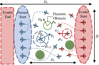
This study considers the swarm confrontation as a pursuit–evasion game where exists dynamic obstacles. There are multiple heterogeneous pursuers to jointly guard the preset target point. They need to work together to capture the same number of evaders as soon as possible while avoiding collisions with obstacles and neighbors. Evaders need to get to the preset target point as quickly as possible without being caught by pursuers, as shown in Fig.1. We use blue and red agents to denote pursuers and evaders, respectively. , , and denote the length and width of the battlefield area and the straight–line distance between the starting areas of both sides, respectively. Let position and velocity vectors in two dimensions be denoted by and , respectively. Pursuers and evaders cannot exceed the boundaries of the scenario and the maximum dynamic constraints, which can be bounded as
| (1) |
where denotes the Euclidean norm. and denote the position of the horizontal and vertical coordinates, respectively. denotes the maximum velocity. Let and denote a swarm of pursuers and evaders, respectively. Both pursuers and evaders should avoid dynamic obstacles . For any pursuer , denotes the capture radius. For any evader , its maximum velocity is greater than the pursuers. We consider and as the radius of agents and obstacles, respectively. In this paper, we design the HRL method for pursuers, while evaders use the expert system approach [10]. The HRL method reflects the commands and actions of the pursuit–evasion game into target allocation and path planning, respectively, through the divide–and–conquer framework approach. We can use to denote the allocation variable which represents whether to allocate to . It yields that
| (2) |
where denotes the allocation matrix for all pursuers. Subsequently, pursuers chase the assigned target through real–time path planning. Throughout the process, target allocation and path planning are dynamically alternated. For pursuers and evaders, we design the rules as follows:
-
1)
Each pursuer is allowed to select only one evader, and one evader can be assigned to several pursuers.
-
2)
If an evader enters the capture radius of one of the pursuers, it is being captured.
-
3)
Both evaders and pursuers that satisfy condition 2) cannot continue moving.
-
4)
The successful condition of pursuers: evaders do not reach the preset target point within the specified time or more than half of evaders are captured.
-
5)
The successful condition of evaders: more than half of evaders can reach the predetermined target point within the time limit without being captured by pursuers.
III-B Markov Decision Process
Let denote the set of real numbers. denotes the mathematical expectation. We can model reinforcement learning by a Markov decision process (MDP). We represent the MDP as a five–tuple . and denote the state of the environment and action of the agent, respectively. denotes the state transition function, denotes the reward function, and denotes the discount factor.
MDP is the case when there is only a single agent or when the system is considered a centralized agent. We can describe a fully cooperative multi–agent reinforcement learning task as a decentralized partially observable Markov decision process (Dec–POMDP). We represent Dec–POMDP as a six–tuple , where the state space , state transition function , reward function and the discount factor have the same denotation as the MDP. For each agent , and denote the action of each agent and the set of the joint actions of all agents, respectively. and denote the observation of each agent and the set of the joint observations of all agents, respectively. is the trajectory of each agent interacting with the environment under the strategy, where and denote the selected action and reaching observation at each decision step , respectively. The purpose of each agent is to optimize the policy network such that the cumulative rewards is maximized under the policy.
IV Main Results
In this section, we introduce the guaranteed stable HRL method for solving the swarm confrontation problem in the dynamic obstacles environment. In the upper layer, it constructs an MDP model and designs a centralized deep Q–learning (DQN) algorithm for the target allocation. In the lower layer, it establishes a Dec–POMDP model and proposes a multi–agent deep deterministic policy gradient (MADDPG) algorithm for path planning. Then, the method feeds the cumulative rewards from the lower to the upper, and adopts a probabilistic ensemble network to quantify the uncertainty caused by unknown evaders’ strategies and moving obstacles. Based on the uncertainty quantification, we use an adaptive truncation method to optimize the interaction frequency between the two layers. In addition, we employ an improved model–based value estimation method to enhance the sample utilization in the upper layer which has fewer samples. Afterward, we design an integration training method including pre–training and cross–training to enhance the training efficiency and stability of our approach.
IV-A Upper Layer for Target Allocation
-
1)
Markov Decision Process. The procedure of the target allocation in the upper layer can be deemed as a sequential decision–making process, where a pursuer will be assigned for each evader. We cast such a process as an MDP which includes state space , action space , reward , and state transition . The detailed definition of our MDP is stated as follows.
-
State. The state mainly consists of the current allocation of all pursuers as well as the information of pursuer that currently needs to be allocated. It can be given as
(3) -
Action. The action consists of the information of the selected evader, which is
(4) -
Reward. Based on the critical model of the target allocation proposed in [10], we get the one–step reward
(5) where denotes the critical model with allocating to .
-
State transition. After pursuer selects evader , becomes one, and it is the turn of pursuer for target allocation.
-
2)
Training method. Combining the above MDP settings, we adopt double DQN for training on target allocation. The method estimates the optimal state–action value function through a parameterized neural network . The subscript is the weighting factor of the neural network. For , estimates the discounted returns of the optimal strategy over an infinite range. The method approximates by and the loss function is set in the following form:
(6) where is the –target. The subscript is a slow–moving online average that avoids overestimation of . At each iteration, it is updated with the following rule:
(7) where is a constant factor. is a replay buffer that iteratively grows as data are updated. We use the same DQN network with a forward inference structure as [39], thus decoupling the network from the size of the problem, which is similar to the critic network in deep deterministic policy gradient (DDPG). Based on centralized DQN, the pursuers maximize the cumulative rewards in (5) with a cooperative approach for optimal target allocation.
IV-B Lower Layer for Path Planning
-
1)
Decentralized Partially Observable Markov Decision Process. Based on the allocation results of the upper layer, each pursuer needs to plan a route to chase the assigned evader and avoid collisions. We model this process as a Dec–POMDP, including the state space , observation space , action space , reward , and state transition :
-
State. The global state space includes information about all pursuers and evaders. It can be described as
(8) -
Observation. The local observation of a pursuer contains the information of the allocated evader, its nearest neighbor and obstacle. It yields that
(9) where and are the position and velocity of the nearest neighbor of pursuer .
-
Action. The action consists of the velocity increment and yaw of each UAV, which is denoted as
(10) -
Reward. To intercept the allocated evader, pursuer receives an intrinsic reward from the upper layer during path planning. The intrinsic reward can be described as
(11) In path planning, pursuers need to avoid collisions with their neighbors and obstacles while chasing their allocated targets. The avoidance reward is set in the following form:
(12) If pursuer enters the threat zone of its nearest obstacle (), there is
(13) otherwise, . And if pursuer enters the threat zone of its nearest neighbor (), there is
(14) otherwise, . are constant rewards. We set a threat distance to avoid collisions between pursuer with its neighbors and obstacles. The total reward for path planning is a linear operation consisting of the intrinsic and avoidance rewards, which is calculated as
(15) -
State transition. Based on the current state and decisions, we can calculate the position at the next moment through the first–order dynamics model
(16) -
2)
Training method. To enable pursuers to make decisions based on local observations while realizing collaboration with each other to accomplish interception, we use the MADDPG algorithm, which is a centralized training with decentralized execution method. It designs a separate critic network for each agent, which is updated similarly to (6) for double DQN as follows:
(17) where . In addition, each agent holds a policy network which has the following loss function:
(18) Based on MADDPG, the pursuers maximize the cumulative rewards in (15) by collaborating while autonomous path planning.
IV-C Hierarchical Network Interaction Method
This study decouples target allocation and path planning into a two–layer networks, and unifies them into a dynamic cyclic process. After time steps in path planning, we need to redo the target allocation based on the current state, where interaction step is a variable related to the current state and allocation . In this dynamic process, the upper layer allocates targets and provides an intrinsic reward to the lower layer, which chases the assigned targets while avoiding obstacles through real–time path planning. To quantify the uncertainty including variant opponents’ strategies and transient battlefield environment, we construct a virtual environment model that incorporates both state transition and reward function, which is expressed as
| (19) |
where denote the predicted value of and with the environment model, respectively. We use an ensemble neural network proposed in [29], which can be used to quantify the epistemic uncertainty and aleatoric uncertainty in the environment. Epistemic uncertainty results from the lack of sufficient training data and aleatoric uncertainty refers to the unknown enemies’ strategies and moving obstacles in this study. It takes the state–action pair as input and outputs Gaussian distribution of the next state and reward. The model can be expressed in the following form:
| (20) |
where and represent the mean and variance of the Gaussian distribution, respectively. This transition dynamics model is trained to maximize the expected likelihood
| (21) |
where represents the model outputs. We omit the inputs of and for brevity. Then, we employ the outputs of sub–models to denote the mean and variance of the ensemble model , which are calculated as
| (22) |
The uncertainty of can be set to the variance of the ensemble model. It is denoted as
| (23) |
Instead of the conventional fixed–step or infinity iteration method, we adopt an adaptive truncation approach, which calculates the prospective value of by the following linear operation:
| (24) |
where is the weighting factor and is an integer limited in . Subscripts , , and are the settled based, minimum, and maximum values, respectively. , where and denotes the set of integers. In [40], it is mentioned that aleatoric uncertainty cannot be reduced with training, but we quantify the uncertainty to adjust the interaction frequency adaptively. When uncertainty is higher, is smaller, indicating the need for more frequent target allocation by the upper layer. As the model fits the environment, the epistemic uncertainty decreases, as well as the frequency of target allocation.
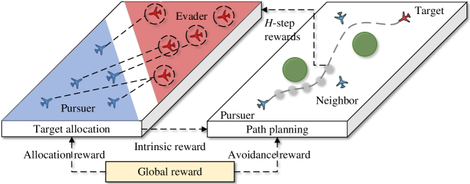
In addition, we feed the cumulative rewards to the upper after the lower executes time steps, as shown in Fig. 2. The upper layer linearly weights the cumulative rewards in (15) and the static allocation reward in (5) as the final reward, which can be denoted as
| (25) |
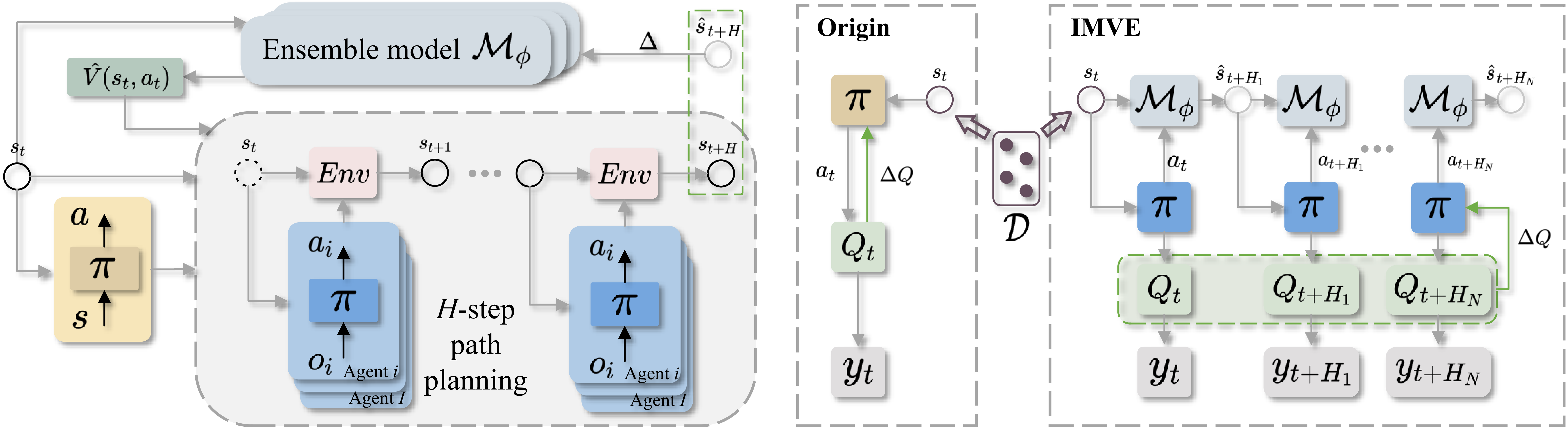
However, samples are greatly reduced since the effect of a single allocation in the upper layer can only be obtained from the feedback of the lower layer planning after steps. Here, we employ an improved model–based value expansion (IMVE) method to improve the sample utilization of the upper layer. The method performs –step value estimation based on the real environment state and allows of steps to converge to . Similar to , is affect by the uncertainty quantified by the model . We can calculate the prospective length of in the following form:
| (26) |
where is an integer limited in . The goal of policy in double DQN is to
maximize the long–term cumulative rewards for all future moments, which can be expressed as
| (27) |
We reduce the prediction interval from infinity to a visual step , and replace the reward with the cumulative rewards in (27). The strategy of IMVE can be described in the following form:
| (28) |
It produces a local optimal solution by performing predictive control based on the single moment . Through rolling iterations at different times, it generates multiple local optimal solutions and calculates the optimal value. The use of cumulative rewards compensates for the lack of the terminal reward. IMVE improves the sample utilization and training efficiency by performing –step value estimation and convergence, the loss function in (6) is improved as follows:
| (29) |
where is defined in the following recursive form:
| (30) |
where . The –target is modified as follows:
| (31) |
In (29), it introduces a discount weight , which is related to the uncertainty of the model with respect to the sample produced. is assigned as follows:
| (32) |
where is limited in . By constructing the environment model , we can quantify the epistemic uncertainty and aleatoric uncertainty, thus allowing , , and to adjust adaptively. Moreover, it allows us to improve the sample utilization of the upper layer based on IMVE. The framework of our method is shown in Fig. 3.
IV-D Integration Training Method
Within the HRL, we design the upper layer and lower layer for target allocation and path planning, respectively. The upper layer assigns targets and intrinsic rewards to the lower layer, and the cumulative rewards of the lower are fed to the upper after time steps. To deal with the strong correlation between the two layers, we propose the integration training method (ITM) consisting of pre–training and cross–training. The training framework is shown in Algorithm 1.
At the beginning of the ITM, we construct the pre–training phase for the upper layer and lower layer for and episodes, respectively. This phase allows the upper layer to learn a static allocation strategy and the lower layer to train an initial path planning policy, which supports the subsequent training phase. After the pre–training phase, we cross–train the two–layer networks for episodes. Since the value of keeps changing according to the state and allocation results , we have to keep it refreshed. Also, the model is keeping updating at the same time in this phase.
Based on this method, we can effectively utilize a large amount of data to learn the initial network in pre–training, thus speeding up the learning process. In addition, it can avoid training instability due to the interactions between the two layers in cross–training.
V Experiments
In this section, extensive experiments are conducted to evaluate the performance of our HRL method for solving the swarm confrontation problem in different sizes. In comparison experiments, we adopt various baselines including the expert system, game theory, heuristic, and traditional DRL algorithms. We verify the influence of adaptive frequency approach and ITM in ablation studies. Moreover, we apply the model trained under a small size to solve larger ones to investigate the generalization of our method.
| Parameter | Upper layer | Lower layer |
| Learning rate | ||
| Discount factor | 0.95 | 0.99 |
| Refresh factor | ||
| Batch size | 120 | 1256 |
| Optimizer | Adam | Adam |
V-A Setting Up
| Method | V10 | V15 | V20 | ||||||
| Re. | Ti.(s) | W.R.(%) | Re. | Ti.(s) | W.R.(%) | Re. | Ti.(s) | W.R.(%) | |
| Expert system | -1521 | 8.26 | 86 | -2603 | 8.89 | 79 | -3610 | 9.67 | 72 |
| Game theory | -1816 | 4.39 | 69 | -2809 | 7.71 | 72 | -3804 | 10.43 | 68 |
| Heuristic | -1564 | 6.45 | 85 | -2435 | 13.58 | 83 | -3302 | 25.30 | 80 |
| DRL | -1703 | 0.49 | 77 | -2847 | 0.73 | 70 | -3786 | 1.06 | 69 |
| UQ-HRL/IMVE | -1182 | 0.86 | 93 | -2091 | 1.20 | 90 | -3078 | 1.87 | 86 |
| UQ-HRL | -1177 | 0.87 | 94 | -2093 | 1.22 | 90 | -3071 | 1.87 | 87 |
Before analyzing the comparative results, we first introduce the detailed settings of simulations. Following the convention in [10, 25, 37], we generate the starting locations of pursuers and evaders in the rectangular area (). The target point of evaders is behind the pursuers. Three scenarios including ten pursuers versus ten evaders (termed as V), fifteen pursuers versus fifteen evaders (termed as V), and twenty pursuers versus twenty evaders (termed as V) are considered in our experiment, all in the presence of four moving obstacles. In each scenario, we set up five different abilities of pursuers and evaders. The capture radius of pursuers is equalized from to . The maximum velocities of pursuers are all set to . The maximum velocities of evaders are equalized from to . The radius of the agents and obstacles are and , respectively.
For algorithm training, we pre–train the upper layer and lower layer for and episodes in randomly generated instances, respectively. The training steps of upper layer are equal to the number of pursuers, and the training steps of lower layer . Then, the cross–training is adopted for episodes in the generated instances above. In this way, we can enhance the training efficiency and stability of the proposed method. We list all the hyperparameters in Table I to demonstrate the details of our algorithm.
V-B Learning Performance in Pre–training
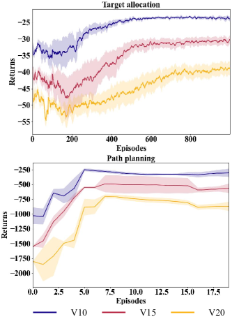
We conduct these simulations on a server with a Windows 10 operating system, Intel Core i7–11700 CPU, 16–GB memory, and Radeon 520 GPU. All simulation programs are developed based on Python 3.7 and PyCharm 2022.2.3 compiler. The learning curves for each scenario of the upper layer and lower layer during the pre–training process are shown in Fig. 4. The horizontal axis refers to the number of episodes. The vertical axis of target allocation and path planning refers to the episode returns calculated by (5) and (15), respectively. To plot experimental curves, we adopt solid curves to depict the mean of all instances and shaded regions corresponding to standard deviation among instances. We can observe that the completely randomized experience replay can lead to performance fluctuations in the initial stage due to the use of the centralized algorithm in the upper layer. Since the rewards of target allocation and path planning are related to the number of agents, the episode returns gradually decrease as the problem size of swarm confrontation increases. The curves for both upper and lower converge stably in different sizes, suggesting that they have learned valid policies. Based on the pre–trained upper layer and lower layer, we can cross–train the two layers and compare our method with other baselines.
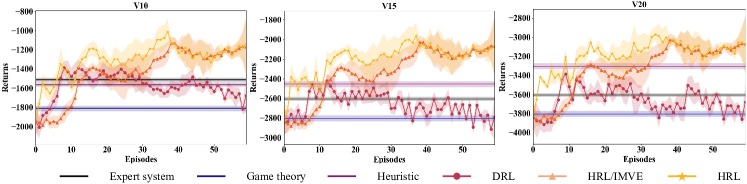
V-C Comparison Analysis in Cross–Training
In the cross–training process, we employ the proposed method to improve the performance of the two layers. We compare the method with the baselines including the expert system, game theory, heuristic approach, and traditional DRL. IMVE adopts a rolling optimization approach to enhance the sample utilization of the upper layer. To investigate the influence of IMVE, we further conduct an ablation study with HRL absent on the IMVE method. The baselines are briefly introduced as follows.
-
1)
Expert system: Based on the rules of the target allocation and path planning in [10], the algorithm can match the optimal action to the current state. Therefore, it is also a rule–based swarm confrontation approach.
-
2)
Game theory: The algorithm models the scenario as a differential game and seeks strategies using Nash equilibrium in a two–coalition non–cooperative game [32], which ultimately obtains the pursuers’ strategies.
-
3)
Heuristic algorithm: The algorithm constructs biologically inspired mobile adaptive networks to imitate the dynamics confrontation of swarms [3]. By building a distributed modular framework that includes target allocation and path planning, pursuers make successive and prompt decisions.
-
4)
DRL: The algorithm considers swarm confrontation as an MDP process and directly employs multi–agent reinforcement learning to output the pursuers’ strategies end–to–end [37].
-
5)
HRL/IMVE: An approach adopts the uncertainty quantification as our HRL method, while it updates the upper layer without IMVE.
The learning curves of HRL and baselines in different–size swarms are presented in Fig. 5. Expert system, game theory, and heuristic algorithms can develop strategies for pursuers in different instances. Among these three non–learning algorithms, game theory performs the worst in uncertainty scenarios. The heuristic algorithm outperforms the expert system algorithm in large–scale swarms. Learning–based algorithms do not perform as well as non–learning algorithms at first due to the randomness of the initial strategy. However, with continuous exploration and training, their performance gradually surpasses the latter. Due to the hybrid decision space in swarm confrontation, the performance of DRL decreases continuously in the later training. In contrast, HRL can find better strategies than non–learning algorithms in different sizes. In addition, with the IMVE method, the performance curve converges in fewer episodes, effectively improving the learning efficiency of HRL.
We further deploy the policy networks trained by the learning–based methods in different instances and compare them with the non–learning algorithms. We propose two additional evaluation metrics: decision time and confrontation win rate. Decision time refers to the total time taken by all pursuers for task allocation and path planning based on their observations. We take the average value after running different instances. The confrontation win rate refers to the ratio of the number of pursuers’ successes to the number of all instances. The experiment results of instances in different sizes are shown in Table II. The table gathers the episode returns (Re.), decision time (Ti.), and confrontation win rate (W.R.) of all methods. We can observe that there is a relationship between the win rate and episode returns, which is calculated by the reward function in this study. The higher the returns achieved by pursuers, then the greater the win rate will be. Among these three non–learning algorithms, the heuristic algorithm has a longer decision time, although its returns and win rate are higher as the problem size increases. Due to the end–to–end approach, DRL has the shortest decision time, but its returns and win rate are much less than HRL. IMVE enhances the training efficiency of the method, but there is no additional improvement in its decision–making performance in the case of policy convergence. As a result, all three metrics for HRL and HRL/IMVE are similar in different scales. The results show that our method achieves better episode returns, decision time, and confrontation win rate than the baselines, especially on large–scale instances. The reason for this is that swarm confrontation in a dynamic obstacle environment has a high degree of uncertainty, and the baselines lack the ability to handle it. Our method optimizes the dynamic mechanism between the two layers based on the probabilistic ensemble model, which quantifies the uncertainty in the scenario.
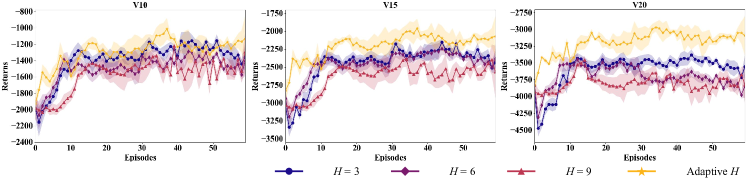
V-D Ablation Study for Adaptive Interaction Frequency
In our method, we construct a probabilistic ensemble model between the upper and lower to quantify the uncertainty. The method optimizes the interaction frequency between the two layers based on the adaptive truncation approach. With adaptive interaction frequency, we construct a dynamic mechanism between target allocation and path planning that enables pursuers to overcome uncertainty while chasing the evaders. To illustrate the effectiveness of the adaptive frequency approach in our method, we conduct an ablation study by fixing interaction step to three sets of constants (). We compare our adaptive method with them in the cross–training process in different scenarios. The learning curves are shown in Fig. 6. When is a constant, the curves first decline for a while, and the decline is greater as is smaller, which means the target is assigned more frequently. This is due to the fact that the upper layer, which is only pre–trained, is less capable of handling uncertainty, and frequent use leads to a drop in performance. When the upper layer has gone through several episodes of cross–training, the curves will eventually converge to sub–optimal values, although they will rise rapidly. Furthermore, the error of sub–optimal values will become larger as the problem size increases.
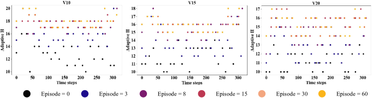
Moreover, we plot the value of for the adaptive method in different sizes and for different episodes (–) of cross–training in Fig. 7. The horizontal coordinate refers to the time steps in each episode, and the vertical coordinate refers to the value of . In the early stage of training, the method decreases the interaction step to augment the training samples in the upper layer. Through constant training, the epistemic uncertainty of the environment model decreases, so the interaction frequency becomes progressively lower. However, since aleatoric uncertainty cannot be eliminated, the increment in stabilizes after episode . In addition, during time steps –, the interaction frequency will be higher than the other time steps because the pursuers will meet with evaders and obstacles, and the aleatoric uncertainty will be higher at this time. Based on the adaptive frequency method, we can overcome the negative effects of uncertainty on cross–training, and finally achieve a favorable training effect.
| Number of | Method | V25 | V30 | V35 | ||||||
| obstacles | Re. | Ti.(s) | W.R.(%) | Re. | Ti.(s) | W.R.(%) | Re. | Ti.(s) | W.R.(%) | |
| 4 | Expert system | -4738 | 10.25 | 69 | -5763 | 11.03 | 66 | -6984 | 12.12 | 62 |
| Game theory | -4799 | 14.17 | 67 | -5905 | 18.89 | 63 | -7149 | 24.32 | 60 | |
| Heuristic | -4186 | 40.82 | 78 | -5094 | 61.34 | 76 | -6027 | 88.73 | 75 | |
| DRL | -4832 | 1.58 | 66 | -5871 | 2.10 | 63 | -6758 | 2.86 | 65 | |
| UQ-HRL | -3911 | 2.41 | 86 | -4862 | 3.05 | 84 | -5703 | 4.20 | 83 | |
| 8 | Expert system | -5392 | 10.89 | 67 | -6499 | 11.94 | 65 | -7841 | 13.17 | 60 |
| Game theory | -5521 | 15.87 | 66 | -6737 | 20.69 | 62 | -8120 | 26.85 | 57 | |
| Heuristic | -4849 | 48.95 | 80 | -5855 | 70.47 | 75 | -6834 | 99.51 | 73 | |
| DRL | -5296 | 1.74 | 68 | -6344 | 2.59 | 66 | -7295 | 3.37 | 65 | |
| UQ-HRL | -4194 | 2.88 | 84 | -5213 | 3.61 | 83 | -6159 | 4.93 | 80 | |
V-E Ablation Study on ITM
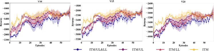
In ITM, we pre–train the upper layer and lower layer based on the rewards referred to (5) and (15), respectively. The pre–training phase allows the upper layer to learn a static allocation strategy and the lower layer to train an initial path planning policy. We conduct an ablation study in the cross–training to investigate the efficiency of pre–training for the upper and lower. The learning curves are shown in Fig. 8, where "ITM/X" refers to adopting ITM but without the pre–training in the "X". For example, ITM/UL denotes the training process only includes the pre–training in the lower layer and cross–training. Due to the lack of pre–training in the upper layer, the training efficiency of ITM/UL is significantly reduced. The curves of ITM/LL first decline for a while, which is attributed to the poor ability of the lower layer that lacks pre–training to deal with uncertainty. The absence of pre–training on two layers leads ITM/UL&LL to perform the worst in cross-training, although it does not affect the final convergence value. Moreover, the effect of pre–training becomes more obvious as the problem size increases. The results verify that ITM can effectively speed up the learning process and avoid training instability.
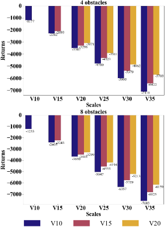
V-F Generalization to Larger–Size Swarms
In larger–scale swarm confrontation scenarios including V25, V30, and V35, we will lose a lot of computational resources by retraining the model. Therefore, we expect the trained model to have favorable generalization performance. We employ the trained two–layer networks to solve the instances with more agents and obstacles to verify the generalization performance of HRL. The models we trained in V10, V15, and V20 are generalized to solve the problem of larger sizes. The generalization results are shown in Fig. 9, where the horizontal axis refers to the scenario sizes, and the vertical axis refers to the episode returns. The legend refers to the model we trained in different sizes. Among scenarios V10–V20, the model trained for a certain size performs best on the corresponding scenario compared to those trained for other sizes. Although models trained on a smaller size have lower returns, they still outperform expert system, game theory, heuristic approach, and DRL. Due to the uncertainty associated with the increase in the number of obstacles, the path planning of the agents becomes more complex and the path reward is reduced. We observe that the model trained in V20 performs best on scenarios V25–V35, since it has a higher capability to handle uncertainty than the other models.
We compare the model trained in V20 with the baselines in scenarios V25–V35 similar to Table II. The experiment results are shown in Table III, which displays the episode returns (Re.), decision time (Ti.), and confrontation win rate (W.R.) testing in different problem sizes. As can be seen, HRL outperforms other baselines in all instances. To further investigate the generalization ability of our method, we utilize the trained model to solve instances with eight obstacles in Table III. An increase in the number of obstacles leads to a decrease in path rewards, but has a very small effect on confrontation win rate. The results demonstrate that the trained policies under small–size swarms are able to deal with the uncertainty in various scale scenarios. Therefore, our method has a strong generalization ability on the swarm confrontation problem.
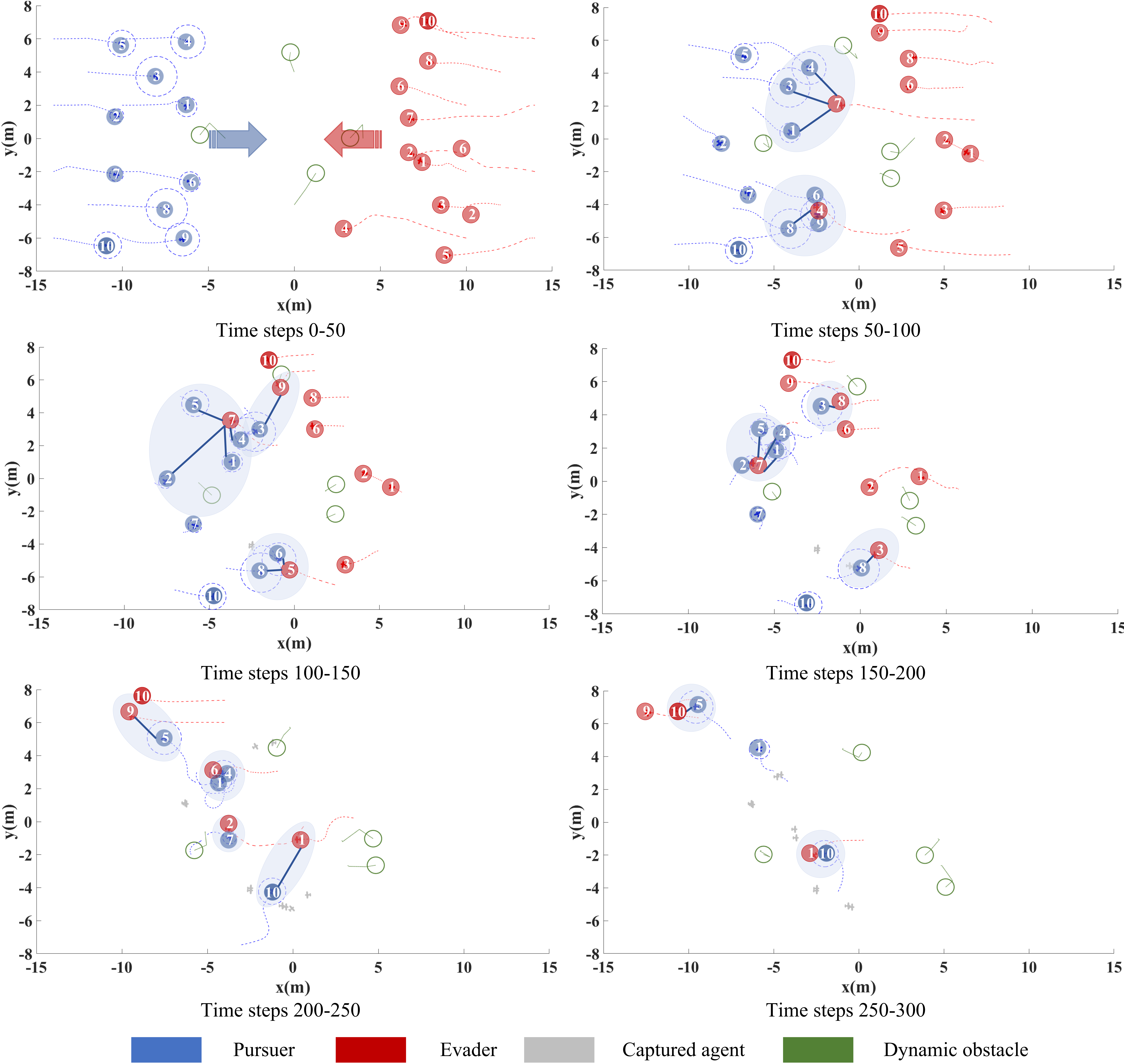
V-G Emerged Coordinated Confrontation Behaviors
With sufficient training from scratch, the proposed HRL method can emerge effective target allocation and path planning strategies. In this section, we visualize the results of trained networks with our method on one of the V10 instances in Fig. 10, and analyze the coordinated behaviors in each stage. Pursuers and evaders are labeled with "" indicating their identification numbers. The figure illustrates the process of target allocation and path planning by pursuers through policy networks at different time steps. In the figure, the upper layer assigns targets based on pursuers’ and evaders’ attributes to maximize the total reward in (25). The lower layer further plans the safe paths to chase evaders while avoiding collisions with obstacles and neighbors.
Time steps –: The upper layer allows for an even target allocation of pursuers to ensure the best possible coverage of the defended area.
Time steps –: After time step , the pursuers begin to encounter evaders and obstacles, introducing more environment uncertainty into decision making. Since pursuers with a large radius have a wider capture range, the upper layer will prioritize mobilizing them to chase evaders with faster escape velocities, such as evader and evader .
Time steps –: In the round–up of evader , the pursuers with a large capture radius surround evader by path planning, and then allow the pursuer with a smaller radius to conduct the final capture. This strategy preserves the pursuers with large radius by sacrificing the ones with smaller radius, which is beneficial to subsequent capture.
Time steps –: After the evaders have escaped the initial round–up by the pursuers, the latter will choose to turn around and chase. The upper layer will assign the pursuers priority to evaders who are closer because they have a higher probability of being captured. Evaders may be hindered by an obstacle or a neighbor ahead, resulting in a loss of velocities, and the pursuers eventually catch up with them.
Time steps –: Even though evader is approaching the target area, the others have been captured by pursuers. According to the rules in Section III, pursuers capture more than half of the evaders, which win the confrontation. Therefore, our trained models could deliver reasonably good solutions in the swarm confrontation.
VI Conclusion
This paper has presented a guaranteed stable HRL method for hybrid decision spaces and high uncertainty in swarm confrontation. It has designed two–layer DRL networks to reflect commands and actions with target allocation and path planning, and quantifies the uncertainty by constructing a probabilistic ensemble model. Furthermore, the method has optimized the interaction mechanism and enhances the sample utilization based on the uncertainty quantification. We have also proposed an integration training method including pre–training and cross–training to enhance the training efficiency and stability. The experiment results have shown that our method achieves better episode returns, decision time, and confrontation win rate than the baselines, especially on large–size swarms. The influence of the adaptive frequency approach and ITM has been verified via ablation studies. Moreover, we have demonstrates the generalization of our method by applying a model trained under small–size swarms to the larger ones. After sufficient training, our method could emerge effective swarm confrontation strategies for agents.
References
- [1] X. Guo, W. Tang, K. Qin, Y. Zhong, H. Xu, Y. Qu, Z. Li, Q. Sheng, Y. Gao, H. Yang et al., “Powerful uav manipulation via bioinspired self-adaptive soft self-contained gripper,” Sci. Adv., vol. 10, no. 19, p. eadn6642, May 2024.
- [2] A. Zhu, T. Dai, G. Xu, P. Pauwels, B. De Vries, and M. Fang, “Deep reinforcement learning for real-time assembly planning in robot-based prefabricated construction,” IEEE Trans. Autom. Sci. Eng., vol. 20, no. 3, pp. 1515–1526, Jul. 2023.
- [3] W. Xia, Z. Zhou, W. Jiang, and Y. Zhang, “Dynamic uav swarm confrontation: An imitation based on mobile adaptive networks,” IEEE Trans. Aerosp. Electron. Syst., vol. 59, no. 5, pp. 7183–7202, Oct. 2023.
- [4] H. Piao, Y. Han, S. He, C. Yu, S. Fan, Y. Hou, C. Bai, and L. Mo, “Spatio-temporal relationship cognitive learning for multi-robot air combat,” IEEE Trans. Cognit. Dev. Syst., vol. 15, no. 4, pp. 2254–2268, Dec. 2023.
- [5] S. Li, C. Wang, and G. Xie, “Optimal strategies for pursuit-evasion differential games of players with damped double integrator dynamics,” IEEE Trans. Autom. Control, early access, Dec., 2023.
- [6] D. Liu, Q. Zong, X. Zhang, R. Zhang, L. Dou, and B. Tian, “Game of drones: Intelligent online decision making of multi-uav confrontation,” IEEE Trans. Emerging Top. Comput. Intell., vol. 8, no. 2, pp. 2086–2100, Dec. 2024.
- [7] T. Zhang, L. Chai, S. Wang, J. Jin, X. Liu, A. Song, and Y. Lan, “Improving autonomous behavior strategy learning in an unmanned swarm system through knowledge enhancement,” IEEE Trans. Reliab., vol. 71, no. 2, pp. 763–774, Jun. 2022.
- [8] Z. Xia, J. Du, J. Wang, C. Jiang, Y. Ren, G. Li, and Z. Han, “Multi-agent reinforcement learning aided intelligent uav swarm for target tracking,” IEEE Trans. Veh. Technol., vol. 71, no. 1, pp. 931–945, Jan. 2021.
- [9] B. Wang, S. Li, X. Gao, and T. Xie, “Weighted mean field reinforcement learning for large-scale uav swarm confrontation,” Appl. Intell., vol. 53, no. 5, pp. 5274–5289, Mar. 2023.
- [10] Y. Hou, X. Liang, J. Zhang, M. Lv, and A. Yang, “Hierarchical decision-making framework for multiple ucavs autonomous confrontation,” IEEE Trans. Veh. Technol., vol. 72, no. 11, pp. 13 953–13 968, Nov. 2023.
- [11] K. G. Vamvoudakis, F. Fotiadis, A. Kanellopoulos, and N.-M. T. Kokolakis, “Nonequilibrium dynamical games: A control systems perspective,” Annu. Rev. Control, vol. 53, pp. 6–18, May 2022.
- [12] J. Kober, J. A. Bagnell, and J. Peters, “Reinforcement learning in robotics: A survey,” Int. J. Robot. Res., vol. 32, no. 11, pp. 1238–1274, 2013.
- [13] E. Kaufmann, L. Bauersfeld, A. Loquercio, M. Müller, V. Koltun, and D. Scaramuzza, “Champion-level drone racing using deep reinforcement learning,” Nature, vol. 620, no. 7976, pp. 982–987, Aug. 2023.
- [14] T. Haarnoja, B. Moran, G. Lever, S. H. Huang, D. Tirumala, J. Humplik, M. Wulfmeier, S. Tunyasuvunakool, N. Y. Siegel, R. Hafner et al., “Learning agile soccer skills for a bipedal robot with deep reinforcement learning,” Sci. Rob., vol. 9, no. 89, p. eadi8022, Apr. 2024.
- [15] B. Eichmann, S. Greiff, J. Naumann, L. Brandhuber, and F. Goldhammer, “Exploring behavioural patterns during complex problem-solving,” J. Comput. Assisted Learn., vol. 36, no. 6, pp. 933–956, Jun. 2020.
- [16] X. Wang, Y. Laili, L. Zhang, and Y. Liu, “Hybrid task scheduling in cloud manufacturing with sparse-reward deep reinforcement learning,” EEE Trans. Autom. Sci. Eng., early access, Mar., 2024.
- [17] X. He and C. Lv, “Robotic control in adversarial and sparse reward environments: A robust goal-conditioned reinforcement learning approach,” IEEE Trans. Artif. Intell., vol. 5, no. 1, pp. 244–253, Jan. 2023.
- [18] M. Eppe, C. Gumbsch, M. Kerzel, P. D. Nguyen, M. V. Butz, and S. Wermter, “Intelligent problem-solving as integrated hierarchical reinforcement learning,” Nat. Mach. Intell., vol. 4, no. 1, pp. 11–20, Jan. 2022.
- [19] X. Mao, G. Wu, M. Fan, Z. Cao, and W. Pedrycz, “Dl-drl: A double-level deep reinforcement learning approach for large-scale task scheduling of multi-uav,” IEEE Trans. Autom. Sci. Eng., early access, Feb., 2024.
- [20] A. S. Vezhnevets, S. Osindero, T. Schaul, N. Heess, M. Jaderberg, D. Silver, and K. Kavukcuoglu, “Feudal networks for hierarchical reinforcement learning,” in Proc. 34th Int. Conf. Mach. Learn. (ICML), vol. 70, Aug. 2017, pp. 3540–3549.
- [21] Y. Guan, Y. Liu, Y. Li, and X. Xu, “Hierrl: Hierarchical reinforcement learning for task scheduling in distributed systems,” in Proceeding of IEEE International Joint Conference on Neural Networks (IJCNN), Sep. 2022, pp. 1–8.
- [22] Y. Ma, X. Hao, J. Hao, J. Lu, X. Liu, T. Xialiang, M. Yuan, Z. Li, J. Tang, and Z. Meng, “A hierarchical reinforcement learning based optimization framework for large-scale dynamic pickup and delivery problems,” in Proc. 33rd Adv. Neural Inf. Process. Syst., vol. 34, 2021, pp. 23 609–23 620.
- [23] Y. Geng, E. Liu, R. Wang, and Y. Liu, “Hierarchical reinforcement learning for relay selection and power optimization in two-hop cooperative relay network,” IEEE Trans. Commun., vol. 70, no. 1, pp. 171–184, Jan. 2021.
- [24] A. Asgharnia, H. M. Schwartz, and M. Atia, “Deception in the game of guarding multiple territories: A machine learning approach,” in Proc. IEEE Int. Conf. Syst. Man Cybern. (SMC), Oct. 2020, pp. 381–388.
- [25] X. Nian, M. Li, H. Wang, Y. Gong, and H. Xiong, “Large-scale uav swarm confrontation based on hierarchical attention actor-critic algorithm,” Appl. Intell., vol. 54, pp. 3279–3294, Feb. 2024.
- [26] B. Wang, S. Li, X. Gao, and T. Xie, “Uav swarm confrontation using hierarchical multiagent reinforcement learning,” Int. J. Aerosp. Eng., vol. 2021, pp. 1–12, Dec. 2021.
- [27] W. Kong, D. Zhou, Y. Du, Y. Zhou, and Y. Zhao, “Hierarchical multi-agent reinforcement learning for multi-aircraft close-range air combat,” IET Control Theory & Appl., vol. 17, no. 13, pp. 1840–1862, Dec. 2023.
- [28] T. Ren, J. Niu, B. Dai, X. Liu, Z. Hu, M. Xu, and M. Guizani, “Enabling efficient scheduling in large-scale uav-assisted mobile-edge computing via hierarchical reinforcement learning,” IEEE Internet Things J., vol. 9, no. 10, pp. 7095–7109, May 2021.
- [29] M. Janner, J. Fu, M. Zhang, and S. Levine, “When to trust your model: Model-based policy optimization,” in Proc.33rd Adv. Neural Inf. Process. Syst., vol. 32, no. 1122, Dec. 2019, pp. 12 519–12 530.
- [30] J. Buckman, D. Hafner, G. Tucker, E. Brevdo, and H. Lee, “Sample-efficient reinforcement learning with stochastic ensemble value expansion,” in Proc.32nd Adv. Neural Inf. Process. Syst., vol. 31, Dec. 2018, pp. 8234–8244.
- [31] L. Wang, T. Qiu, Z. Pu, J. Yi, J. Zhu, and Y. Zhao, “A decision-making method for swarm agents in attack-defense confrontation,” 22nd IFAC World Congress, vol. 56, no. 2, pp. 7858–7864, Nov. 2023.
- [32] F. Liu, X. Dong, J. Yu, Y. Hua, Q. Li, and Z. Ren, “Distributed nash equilibrium seeking of -coalition noncooperative games with application to uav swarms,” IEEE Trans. Network Sci. Eng., vol. 9, no. 4, pp. 2392–2405, Jul.–Aug. 2022.
- [33] H. Liu, J. Zhang, P. Zu, and M. Zhou, “Evolutionary algorithm-based attack strategy with swarm robots in denied environments,” IEEE Trans. Evol. Comput., vol. 27, no. 6, pp. 1562–1574, Dec. 2023.
- [34] P. R. Wurman, P. Stone, and M. Spranger, “Challenges and opportunities of applying reinforcement learning to autonomous racing,” IEEE Intelligent Systems, vol. 37, no. 3, pp. 20–23, May–Jun. 2022.
- [35] L. Gao, J. Schulman, and J. Hilton, “Scaling laws for reward model overoptimization,” in Proc. 40th Int. Conf. Mach. Learn. (ICML), no. 437, Jul. 2023, pp. 10 835–10 866.
- [36] C. De Souza, R. Newbury, A. Cosgun, P. Castillo, B. Vidolov, and D. Kulić, “Decentralized multi-agent pursuit using deep reinforcement learning,” IEEE Rob. Autom. Lett., vol. 6, no. 3, pp. 4552–4559, Jul. 2021.
- [37] X. Qu, W. Gan, D. Song, and L. Zhou, “Pursuit-evasion game strategy of usv based on deep reinforcement learning in complex multi-obstacle environment,” Ocean Eng., vol. 273, p. 114016, Feb. 2023.
- [38] W. Kong, D. Zhou, Y. Zhou, and Y. Zhao, “Hierarchical reinforcement learning from competitive self-play for dual-aircraft formation air combat,” J. Comput. Des. Eng., vol. 10, no. 2, pp. 830–859, Apr. 2022.
- [39] W. Luo, J. Lü, K. Liu, and L. Chen, “Learning-based policy optimization for adversarial missile-target assignment,” IEEE Trans. Syst. Man Cybern.: Syst., vol. 52, no. 7, pp. 4426–4437, Jul. 2021.
- [40] K. Chua, R. Calandra, R. McAllister, and S. Levine, “Deep reinforcement learning in a handful of trials using probabilistic dynamics models,” in Proc. 32nd Adv. Neural Inf. Process. Syst., vol. 31, 2018, p. 4759–4770.
| Qizhen Wu received the B.S. degree in aeronautical and astronautical engineering from Sun Yat–sen University, Guangzhou, China, in 2022. He is currently pursuing the master degree with the School of Automation Science and Electrical Engineering, Beihang University, Beijing, China. His current research interests include reinforcement learning, robotic control, and swarm confrontation. |
| Kexin Liu received the M.Sc. degree in control science and engineering from Shandong University, Jinan, China, in 2013, and the Ph.D. degree in system theory from the Academy of Mathematics and Systems Science, Chinese Academy of Sciences, Beijing, China, in 2016. From 2016 to 2018, he was a Postdoctoral Fellow with Peking University, Beijing. He is currently an Associated Professor with the School of Automation Science and Electrical Engineering, Beihang University, Beijing. His current research interests include multiagent systems and complex networks |
| Lei Chen received the Ph.D. degree in control theory and engineering from Southeast University, Nanjing, China, in 2018. He was a visiting Ph.D. student with the Royal Melbourne Institute of Technology University, Melbourne, VIC, Australia, and Okayama Prefectural University, Soja, Japan. From 2018 to 2020, he was a Postdoctoral Fellow with the School of Automation Science and Electrical Engineering, Beihang University, Beijing, China. He is currently with the Advanced Research Institute of Multidisciplinary Science, Beijing Institute of Technology, Beijing, as an Associate Research Fellow. His current research interests include complex networks, characteristic model, spacecraft control, and network control. |
| Jinhu Lü (Fellow, IEEE) received the Ph.D. degree in applied mathematics from the Academy of Mathematics and Systems Science, Chinese Academy of Sciences, Beijing, China, in 2002. He was a Professor with RMIT University, Melbourne, VIC, Australia, and a Visiting Fellow with Princeton University, Princeton, NJ, USA. He is currently the Dean of the School of Automation Science and Electrical Engineering, Beihang University, Beijing. He is also a Professor with the Academy of Mathematics and Systems Science, Chinese Academy of Sciences. He is a Chief Scientist of the National Key Research and Development Program of China and a Leading Scientist of Innovative Research Groups of the National Natural Science Foundation of China. His current research interests include complex networks, industrial Internet, network dynamics, and cooperation control. Prof. Lü was a recipient of the Prestigious Ho Leung Ho Lee Foundation Award in 2015, the National Innovation Competition Award in 2020, the State Natural Science Award three times from the Chinese Government in 2008, 2012, and 2016, respectively, the Australian Research Council Future Fellowships Award in 2009, the National Natural Science Fund for Distinguished Young Scholars Award, and the Highly Cited Researcher Award in engineering from 2014 to 2020. He is/was an Editor in various ranks for 15 SCI journals, including the Co-Editor-in-Chief of IEEE TRANSACTIONS ON INDUSTRIAL INFORMATICS. He served as a member in the Fellows Evaluating Committee of the IEEE CASS, the IEEE CIS, and the IEEE IES. He was the General Co-Chair of IECON 2017. He is a Fellow of CAA |