Bridging multiple worlds: multi-marginal optimal transport for causal partial-identification problem

Abstract

Under the prevalent potential outcome model in causal inference, each unit is associated with multiple potential outcomes but at most one of which is observed, leading to many causal quantities being only partially identified. The inherent missing data issue echoes the multi-marginal optimal transport (MOT) problem, where marginal distributions are known, but how the marginals couple to form the joint distribution is unavailable. In this paper, we cast the causal partial identification problem in the framework of MOT with $K$ margins and $d$-dimensional outcomes and obtain the exact partial identified set. In order to estimate the partial identified set via MOT, statistically, we establish a convergence rate of the plug-in MOT estimator for general quadratic objective functions and prove it is minimax optimal for a quadratic objective function stemming from the variance minimization problem with arbitrary $K$ and $d\leq 4$. Numerically, we demonstrate the efficacy of our method over several real-world datasets where our proposal consistently outperforms the baseline by a significant margin (over 70%). In addition, we provide efficient off-the-shelf implementations of MOT with general objective functions.

1 Introduction

The potential outcome model [35] has been extensively used to perform causal inference. Suppose there are $K$ possible treatment levels, and each unit $i$ is associated with $K$ potential outcomes $\mathbf{Y}_{i}(\cdot)=(Y_{i}(1),\ldots,Y_{i}(K))$ with $Y_{i}(k)=(Y_{i}^{1}(k),\ldots,Y_{i}^{d}(k))$, drawn independently from an unknown joint distribution $\mu_{\star}$. The interest lies in assessing the impact of a treatment $W$ on the outcomes.

The fundamental challenge of causal inference is that we can only observe the potential outcome $Y_{i}=Y_{i}(W_{i})$ at the realized treatment level $W_{i}$, and it is impossible to observe the entire set of $K$ potential outcomes. As a consequence, the marginal distribution $\mu_{\star}(k)$ of $Y_{i}(k)$, $1\leq k\leq K$ can be identified but how the marginals $\mu_{\star}(k)$ couple to form the full joint distribution $\mu_{\star}$ is not identified. This renders a large class of causal estimands relying on the joint distribution $\mu_{\star}$ to be only partially identifiable, and examples include $\mathsf{Var}_{\mu_{\star}}(Y_{i}(2)-Y_{i}(1))$ for assessing the treatment effect heterogeneity [7], $\mathbb{P}_{\mu_{\star}}(Y_{i}(2)-Y_{i}(1)\leq y)$ describing the distribution of the individual treatment effect $Y_{i}(2)-Y_{i}(1)$ [14], and $\mathsf{Cov}_{\mu_{\star}}\left(Y_{i}^{1}(2)-Y_{i}^{1}(1),Y_{i}^{2}(2)-Y_{i}^{2}(1)\right)$ representing the covariance between individual treatment effects across different dimensions of the outcome. For partially-identified causal estimands, the statistical task is determining the identified set: the full set of values that are compatible with the observed data.

Optimal transport, particularly Multi-margin Optimal Transport (MOT) when there are more than two margins, is a fast-growing research area partly due to the emerging applications in machine learning including networks (GANs) [9], domain adaptation [18], and Wasserstein barycenters [1]. The MOT problem considers a cost (objective) function of random variables with known marginal distributions and seeks to find the coupling of the marginal distributions that minimizes the expected cost [32]. In addition to the optimal coupling, MOT outputs the exact lower bound of the expected cost among all joint distributions obeying the marginal distributions, even if the optimal coupling is not unique.

This paper addresses the partial identification problem under the potential outcome model using MOT. In a nutshell, the partially identified problem resembles the MOT in the sense that the marginal distribution of each potential outcome is identifiable but the joint distribution can not be uniquely determined. For a causal estimand, we can devise an MOT problem whose optimal objective value corresponds to the lower (upper) limit of the causal quantity that can be achieved by some joint distribution respecting the identifiable marginals.

1.1 Overview and contributions

In this paper, we investigate solving for partially identified sets of causal estimands using MOT. Let $\Gamma$ represent the collection of joint probabilities respecting the marginal distributions $\mu_{\star}(k)$, $1\leq k\leq K$. For a causal estimand of the form $\mathbb{E}_{\mu_{\star}}[\ell(\bm{Y}_{i}(\cdot))]$, where $\ell$ can depend on all potential outcomes, the identified set can be expressed as

$$\left\{\mathbb{E}_{\gamma}[\ell(\bm{Y}_{i}(\cdot))]:\gamma\in\Gamma\right\}.$$

Since $\Gamma$ is convex by definition and the estimand $\mathbb{E}_{\gamma}[\ell(\bm{Y}_{i}(\cdot))]$ is linear in $\gamma$, the identified set is always an interval

$$\left[\inf_{\gamma\in\Gamma}\mathbb{E}_{\gamma}[\ell(\bm{Y}_{i}(\cdot))],~{}\sup_{\gamma\in\Gamma}\mathbb{E}_{\gamma}[\ell(\bm{Y}_{i}(\cdot))]\right].$$ (1)

The task of determining the identified set reduces to calculating the lower and upper limits, which can be obtained by solving two MOT problems. See Figure 1 for visualization.

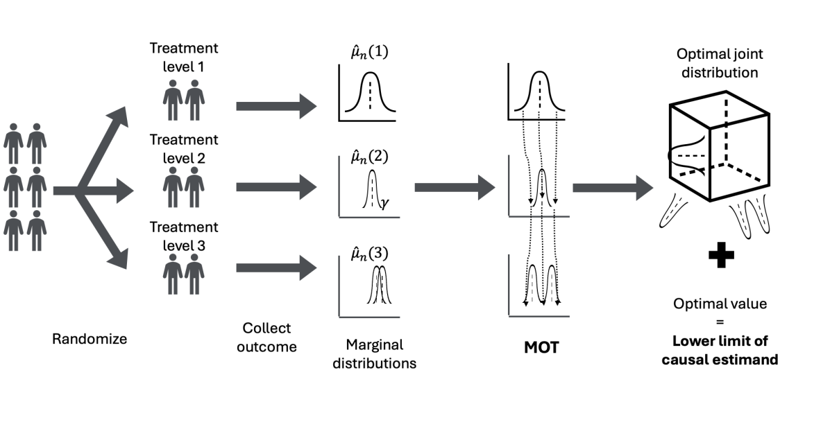
Figure 1: Diagram of solving partial identification problem via MOT. A treatment with multiple levels is applied to a group of individuals. The outcomes of each treatment group are collected to form the empirical marginal distribution denoted by $\hat{\mu}_{n}(k)$, $1\leq k\leq K$. An MOT problem with the causal estimand as the objective function and empirical marginal distributions as the constraints are solved to obtain the lower limit of the partially identified set. The upper limit can be obtained similarly by flipping the sign of the MOT objective function.

Our contributions are three-fold.

1. Our proposal recovers the exact partially identified set given the true marginal distributions. Our proposal can accommodate various scenarios including multiple treatment levels, multiple treatments, and multiple outcomes (see Section 2 for examples). Across various real datasets, we demonstrate that our method achieves an improvement of approximately $70\%$ or more compared to a baseline approach (Section 2). In addition, our method can be used to derive the sharp variance upper bound for design-based estimators, improving the conventional Neyman’s variance estimator [37].

2. In practice, we propose to use the plug-in estimator associated with the MOT problem with the true marginal distributions replaced by the empirical marginal distributions. We provide an upper bound on the estimation error of the plug-in estimator for arbitrary quadratic losses. In particular, for $d\leq 4$ and using the $\ell_{2}$ norm of the average potential outcomes as the objective, we show the plug-in estimator converges at the parametric rate $O(n^{-1/2})$ up to logarithmic terms. Surprisingly, the rate is independent of the number of margins $K$. In addition, we provide a matching lower bound, demonstrating that the plug-in estimator is minimax optimal for the aforementioned particular case. The proof techniques involved, as elaborated in Section 3, could be of independent interest.

3. For implementation, we provide several solvers of MOT, addressing the lack of efficient off-the-shelf MOT packages. In particular, we employ the celebrated log-sum-exp trick to increase numerical stability, which is exacerbated by the number of margins (since the number of cell probabilities scales exponentially with the number of margins). Additionally, our algorithm provides valid lower bounds of the optimal (minimal) objective value across iterations before convergence, thereby always providing valid, albeit conservative, partially identified sets.

1.2 Related works

1.2.1 Partial-identification

In the literature of causal inference, identifiability is typically the first issue addressed when a new causal estimand is proposed. Under the potential outcome model, causal estimands depending on cross-world potential outcomes are generally not identifiable due to the inherent missingness. In this case, the range of parameter values that are compatible with the data is of interest. A multitude of works have been dedicated to finding causal estimands that can be identified, where a set of assumptions is usually necessary. For instance, the identifiability of the average treatment effect requires the assumption of no unobserved confounders, and using instrumental variables to identify the local treatment effect requires the exogeneity [20]. However, verifying these assumptions can be challenging or even impossible based solely on the data, and the violation of the assumptions will render the parameter unidentified.

In the literature of econometrics, the partial identification problem has been a topic of heated discussion for decades (see [24] for a comprehensive review and references therein). The works generally begin with a model depending on the parameter of interest and possibly other nuisance parameters or functions. The partially identified sets are specified to be the values that comply with a set of moment inequalities, parameters that maximize a target function, or intervals with specifically defined endpoints. In causal inference, there is a tendency to avoid heavy model assumptions imposed on the potential outcomes to ensure the robustness and generalizability of causal conclusions. Methods therein often involve leveraging non-parametric or semi-parametric methods that make few structural assumptions about the data-generating process [6, 41, 25].

We detail two particularly relevant threads of works among the studies on partial identification problems. Copula models [31] are used to describe the dependency between multiple random variables with known marginal distributions, which also aligns with the potential outcome model with marginals accessible and the coupling unknown. The Fréchet–Hoeffding copula bounds can be used to characterize the joint distribution of the potential outcomes [17, 30, 12]. However, when dealing with more than two margins, one side of the Fréchet–Hoeffding theorem’s bound is only point-wise sharp; moreover, copula models are generally constrained to unidimensional random variables; in addition, the bounds on the joint distribution do not necessarily translate to those of causal estimands, such as the variance of the difference of two potential outcomes. The second thread of related works explicitly employs the optimal transport, specifically its dual form, to address the partial identification problem in econometrics [15]. This approach considers a model that includes observed variables and latent variables, and the parameter of interest regulates the distribution of the latent variables and the relationship between the observed and unobserved variables, which differ from our problem formulation.

1.2.2 MOT

MOT and minimax estimation

The convergence of the empirical optimal transport cost (with two margins) to its population value has been extensively and thoroughly researched (see [8, 38, 29] and the references therein). Moreover, the estimation error of the plug-in estimator (i.e., the empirical optimal transport cost) is known to be minimax optimal for Wasserstein $p$-cost. However, to the best of our knowledge, such minimax results have not been established for the MOT problem. In this paper, we generalize the approach by [8] to provide a convergence result for the plug-in estimator of the MOT problem for arbitrary quadratic objective functions (Eq. (2)). Furthermore, we refine the analysis for the average squared $\ell_{2}$ norm (Eq. (3)) and show that the plug-in estimator is minimax optimal when the dimension $d\leq 4$. Determining the minimax rates for cases where $d>4$, and for arbitrary quadratic functions remains an interesting direction for future research.

Computation for MOT

For computing Optimal Transport (OT) distance, the Sinkhorn algorithm [10] and its accelerated variants (see [2, 26, 47] and references therein) remain the state-of-the-art approach. Extensions of the Sinkhorn algorithm to the MOT problem have been proposed in the literature [33, 40, 27]. Notably, [40, 27] provide finite time convergence guarantees for the Multi-marginal Sinkhorn and Primal-Dual Accelerated Alternating Minimization (PD-AAM) algorithms, respectively. While the implementations of OT algorithms are quite advanced [13], those for MOT algorithms are still in the early stages. Specifically, [40] offers implementations that work with $K=4$, $n=60$ and accuracy $\epsilon=1/80$. Since our tasks require concrete lower bounds for the MOT problem at a considerably larger scale of sample size $n$ and higher accuracy $\epsilon$, we have implemented several algorithms (see Section 4.1 for details), used them to obtain our numerical results, and provided an efficient off-the-shelf MOT package.

Organization

The paper is organized as follows. In Section 2, we fix notations and frame various causal partially identified set problems as a MOT problem. In Section 3, we investigate the estimation accuracy of the plug-in estimator of the MOT problem. In Section 4, we discuss implementations and application results on real world datasets. In Section 5, we conclude the paper by discussing potential research directions stemming from the current work.

2 MOT formulation of partial identification problem

We recall briefly the relevant notations. We denote by $\bm{Y}_{i}(\cdot)$ the potential outcomes of unit $i$. At treatment level $k$, the potential outcome is denoted by $Y_{i}(k)=(Y_{i}^{1}(k),...,Y_{i}^{d}(k))\in\mathbb{R}^{d}$. Let $\mu_{\star}$ be the joint distribution that are only partially identifiable and $\mu_{\star}(k)$ be its $k$-th margin for $k\in[K]$. Without loss of generality, we suppose the marginals $\mu_{\star}(k)$ for any $k\in[K]$ are supported on $B_{1}^{d}(0)\subset\mathbb{R}^{d}$ which is the $d$-dimensional unit ball.

We explore three types of objectives in the increasing order of specificity (Table 1).

Table 1: Summary of results for different objective functions.

Objective function	Theoretical properties	Computation
Arbitrary quadratic function	Upper bound (Proposition 3.1)	Algorithm 2 with provable convergence
Average squared $\ell_{2}$ norm	Upper bound (Theorem 3.1), lower bound (Proposition 3.2)

2.1 Arbitrary function

In Section 1, we described the causal partial identification problem where the parameter of interest is the expectation of an arbitrary objective function $\ell$. For the two-margin optimal transport with general objective function, the convergence of the empirical optimal transport cost has been established for smooth objective functions with compact supports [19], objectives of the form $\ell(y(2)-y(1))$ [29], or under bounded moment assumptions [38]. To the authors’ knowledge, the convergence results for general MOT cost has not been explicitly stated. For the rest of the paper, we will focus on quadratic objective functions that possess favorable statistical properties and admit various applications.

2.2 Arbitrary quadratic function

Quadratic objective functions are practically useful (as demonstrated in the examples below) and the estimation error analysis can be helped by the quadratic structure. Let $A\in\mathbb{R}^{K\times K}$ be a symmetric matrix and recall that $\Gamma(\mu_{\star}(1),...,\mu_{\star}(K))$ denotes the set of all possible couplings of $\mu_{\star}(1),...,\mu_{\star}(K)$, i.e., distributions $\gamma$ where the $k$-th margin $\gamma(k)$ is equal to $\mu_{\star}(k)$ for all $k\in[K]$. We define the quadratic objective parametrized by $A$ as

$$\mathrm{QMW}(\mu_{\star};A)=\mathrm{QMW}(\mu_{\star}(1),\dots,\mu_{\star}(K);A):=\inf_{\gamma\in\Gamma(\mu_{\star}(1),\dots,\mu_{\star}(K))}\int y^{\top}Ay~{}\gamma(dy).$$ (2)

2.3 Average squared $\ell_{2}$ norm

Specifically, we focus on the following quadratic form which is flexible enough to encompass most of our examples of interest (Examples 2.3 and 2.1) as well as objectives in existing literature detailed below. Concretely, we define

$$\mathrm{MW}_{2}^{2}(\mu_{\star})=\mathrm{MW}_{2}^{2}(\mu_{\star}(1),\ldots,\mu_{\star}(K)):=\inf_{\gamma\in\Gamma(\mu_{\star}(1),\dots,\mu_{\star}(K))}\int\left\|\frac{\sum_{k=1}^{K}y(k)}{K}\right\|_{2}^{2}~{}\gamma(dy),$$ (3)

where the objective function in Eq. (3) corresponds to the integral of the squared $\ell_{2}$ norm of the average potential outcome $(\sum_{k=1}^{K}y(k))/K$. This objective is a special case of in (2) with $A=(a_{ij}=1/K^{2})_{1\leq i,j\leq K}$.

The quantity $\mathrm{MW}_{2}^{2}(\mu_{\star})$ has multiple connections to the existing literature. For instance, the expected sum of pairwise squared Wasserstein distance $\sum_{k\neq k^{\prime}}\mathbb{E}_{\mu_{\star}}[(Y_{i}(k)-Y_{i}(k^{\prime}))^{2}]$ is related to the repulsive harmonic cost arising from the weak interaction regime in Quantum Mechanics [11] and can be written as $K^{2}\mathrm{MW}_{2}^{2}(\mu_{\star})$ subtracted from the estimable quantity $2K\sum_{k=1}^{K}\mathbb{E}_{\mu_{\star}(k)}[(Y_{i}(k))^{2}]$. Another example is variance minimization problem [36], where the minimum variance can be written as $K^{2}\mathrm{MW}_{2}^{2}(\mu_{\star})$ subtracting the estimable quantity $(\sum_{k=1}^{K}\mathbb{E}_{\mu_{\star}(k)}[Y_{i}(k)])^{2}$. Lastly, one metric to quantify the heritability in genetic studies [21] is defined as $\mathbb{E}_{\mu_{\star}}[\mathsf{Var}(Y_{i}(W_{i})\mid\bm{Y}_{i}(\cdot))]$, or equivalently $\mathbb{E}_{\mu_{\star}}[Y_{i}^{2}(W_{i})]-\mathbb{E}_{\mu_{\star}}[(\sum_{k=1}^{K}Y_{i}(k)\mathbb{P}(W_{i}=k))^{2}]$. The upper bound of the metric can be obtained by solving a modified version of Eq. (3) incorporating the weights $\mathbb{P}(W_{i}=k)$.

We describe a non-tight lower bound of the objective Eq. (3), which serves as the baseline to compare with. The objective Eq. (3) admits the following decomposition (Lemma B.1),

$$\mathrm{MW}_{2}^{2}(\mu_{\star})=\left\|\frac{\sum_{k=1}^{K}\mathbb{E}_{\mu_{\star}(k)}[Y_{i}(k)]}{K}\right\|_{2}^{2}+\mathrm{MW}_{2}^{2}(\bar{\mu}_{\star}),$$ (4)

where $\bar{\mu}_{\star}$ denotes the centered counterpart of ${\mu}_{\star}$, that is, $\bar{\mu}_{\star}(k)$ is a translation of $\mu_{\star}(k)$ by $-\mathbb{E}_{\mu_{\star}(k)}\left[Y_{i}(k)\right]$. The first term on the right-hand side of Eq. (4) depends solely on the first moment of each margin, and the second term contains the information of higher-order moments. Since $\mathrm{MW}_{2}^{2}(\bar{\mu}_{\star})$ is non-negative, the first term is a straightforward lower bound of $\mathrm{MW}_{2}^{2}(\mu_{\star})$, which we refer to as the baseline lower bound. When $\mathrm{MW}_{2}^{2}(\bar{\mu}_{\star})$ is zero, i.e., $\mu_{\star}(k)$ satisfying the joint mixability property [45], the baseline lower bound is adequate. When the marginal distributions differ in second or higher-order moments, the baseline is not sufficient and our method offers a potentially significantly tighter lower bound (see Section 4.2 for real data demonstrations).

2.4 Examples

In this paper, we are interested in the following examples of causal partial-identification that can be formulated in terms of the objective in Eq. (3) or (2).

Example 2.1 (Detection of treatment effect).

Our proposal can be applied to detect the interaction effect of multiple treatments. Suppose there are two binary treatments. We use $Y_{i}(0,0)$ to denote the potential outcome under control of both treatments, and similarly for $Y_{i}(0,1)$, $Y_{i}(1,0)$, $Y_{i}(1,1)$, and the potential outcomes $Y_{i}(\cdot)=(Y_{i}(1,1),-Y_{i}(1,0),-Y_{i}(0,1),Y_{i}(0,0))$ possess four margins in total. Identifying a non-zero interaction treatment effect, i.e., $Y_{i}(1,1)-Y_{i}(1,0)-Y_{i}(0,1)+Y_{i}(0,0)\neq 0$, is crucial as it can facilitate the detection of drug synergy (whether different drugs’ combined effect is greater than the sum of their individual effects). The tight lower bound of $\mathbb{E}_{\mu_{\star}}[(Y_{i}(1,1)-Y_{i}(1,0)-Y_{i}(0,1)+Y_{i}(0,0))^{2}]$ can be solved for as in Eq. (3), and a significantly positive lower bound suggests the existence of interaction effect.

The above method can also be applied to detect the contrast effect of a treatment with multiple levels. Suppose there is a treatment with $K$ levels, and the corresponding potential outcomes are associated with $K$ margins. Unlike the case of a binary treatment, there are various ways to define an estimand for treatments of multiple levels, and a popular choice is considering a contrast vector $\bm{\beta}\in\mathbb{R}^{k}$, $\sum_{k=1}^{K}\beta_{k}=0$ and the associated contrast treatment effect $\sum_{k=1}^{K}\beta_{k}{Y}_{i}(k)$. Similar to the interaction effect, a significantly positive lower bound of $\mathbb{E}_{\mu_{\star}}[(\sum_{k=1}^{K}\beta_{k}{Y}_{i}(k))^{2}]$ is a sign to reject the null hypothesis of no contrast effect.

We remark that standard methods for testing the existence of treatment effects construct a confidence interval for the treatment effect estimator $\sum_{i=1}^{n}(n/K)^{-1}\sum_{k=1}^{K}\beta_{k}\mathbbm{1}_{\{W_{i}=k\}}Y_{i}$ [20]. The standard approach is related to testing whether the baseline lower bound in (4) is significantly greater than zero. In comparison, our method uses the sharp lower bound and is potentially more powerful.

Example 2.2 (Covariance between treatment effects).

The covariance between treatment effects of different dimensions of the outcomes $\mathsf{Cov}_{\mu_{\star}}(\tau^{1}_{i},\tau^{2}_{i})$ with $\tau_{i}^{j}=Y_{i}^{j}(2)-Y_{i}^{j}(1)$, $j=1$, $2$ takes the form of Eq. (2) and its upper and lower bounds can be obtained by solving the corresponding MOT problems.

By investigating the exact lower and upper bounds of the covariance, we provide a model-free way to detect positively or negatively associated treatment effects (Section 4.3). There are many relevant applications in economics, e.g., the effects of a promotion scheme on the sale of complementary goods shall be positively correlated, and social sciences, e.g., the effects of a subsidy program on the full-time employment and part-time employment rate, might be negatively correlated.

Example 2.3 (Neymanian confidence interval).

Another thread of causal inference research, known as design-based methods, focuses on finite samples rather than superpopulations. The potential outcomes are considered fixed and the randomness for inference comes from the treatment assignment or experiment design. Particularly, consider the average contrast effect estimand ${\tau}_{\bm{\beta}}:=\sum_{k=1}^{K}\beta_{k}\bar{Y}(k)$ following from Example 2.1, where $\bar{Y}(k)=\sum_{i=1}^{n}{Y}_{i}(k)/n$, and the difference-in-means type estimator $\hat{\tau}_{\bm{\beta}}:=\sum_{k=1}^{K}\beta_{k}(\sum_{W_{i}=k}Y_{i}(k)/n_{k})$ from a completely randomized experiment with $n_{k}$ units at treatment level $k$. The construction of Neymanian confidence interval [37] for ${\tau}_{\bm{\beta}}$ based on $\hat{\tau}_{\bm{\beta}}$ requires the variance of $\hat{\tau}_{\bm{\beta}}$ of the form [28]

$$,\begin{split}V_{\bm{\beta}}:=&\sum_{k=1}^{K}\frac{\beta_{k}^{2}S_{k}^{2}}{(n/K)}-\frac{S_{\tau}^{2}}{n},\\ S_{k}^{2}=\frac{\sum_{i=1}^{n}(Y_{i}(k)-\bar{Y}(k))^{2}}{n-1}&,~{}S_{\tau}^{2}=\frac{\sum_{i=1}^{n}(\sum_{k=1}^{K}\beta_{k}Y_{i}(k)-\tau_{\bm{\beta}})^{2}}{n-1}.\end{split}$$ (5)

The conventional variance estimator of $V_{\bm{\beta}}$ replaces $S_{k}^{2}$ by the empirical variance among units receiving $W_{i}=k$ and simply lower bounds $S_{\tau}^{2}$ by zero.

Note that $S_{\tau}^{2}$ is precisely the objective in Eq. (3) with the marginal distribution of $K\beta_{k}\cdot Y_{i}(k)$, $1\leq k\leq K$ minus the estimable contrast mean squared $\left\|{\sum_{k=1}^{K}\mathbb{E}_{\mu_{*}(k)}[\beta_{k}Y_{i}(k)]}\right\|_{2}^{2}$. The trivial lower bound zero is equivalent to the baseline lower bound in (4). Our proposal can be used to provide a tight lower bound of $S_{\tau}^{2}$ and asymptotically narrowest conservative confidence intervals for causal estimators, extending previous results of the sharp confidence interval for a binary treatment [5]. Here, a narrower confidence interval may imply that a smaller sample size is required in the corresponding clinical trial and reduces the associated costs.

3 Theoretical characterization of the estimation error

In this section, we consider the minimax estimation error of the value $\mathrm{MW}_{2}^{2}(\mu_{\star})$ and $\mathrm{QMW}(\mu_{\star};A)$ with $n$ empirical samples. Concretely, suppose we have $n$ i.i.d. samples from the distribution $\mu_{\star}$ and assigned $n/K$ samples to each treatment level $k$. For simplicity, we assume $n/K$ is an integer. Specifically, suppose we have samples $\{Y_{i}(k)\}_{i\in[n/K],k\in[K]}$. Let the empirical distribution be $\hat{\mu}_{n}=(\hat{\mu}_{n}(1),...,\hat{\mu}_{n}(K))$, where $\hat{\mu}_{n}(k)=\mathrm{Unif}(\{Y_{i}(k)\}_{i\in[n/K]})$. In Section 3.1, we establish the parametric rate of convergence for $\mathrm{MW}_{2}^{2}(\hat{\mu}_{n})$ to $\mathrm{MW}_{2}^{2}(\mu_{\star})$ for $d\leq 4$ and convergence result for $\mathrm{QMW}(\hat{\mu}_{n};A)$ to $\mathrm{QMW}(\mu_{\star};A)$, respectively. Then we present a matching minimax lower bound for the estimation error of $\mathrm{MW}_{2}^{2}(\mu_{\star})$ when $d\leq 4$ in Section 3.2.

3.1 Upper bound

In this section, we prove finite sample upper bounds for the convergence of $\mathrm{MW}_{2}^{2}(\hat{\mu}_{n})$ and $\mathrm{QMW}(\hat{\mu}_{n};A)$ to $\mathrm{MW}_{2}^{2}(\mu_{\star})$ and $\mathrm{QMW}(\mu_{\star};A)$, respectively. Similar convergence results have been shown for optimal transport [8]. Their approach first considers the dual formulation of the optimal transport. Then, by noticing the earth’s moving distance is quadratic, they proceed to formulate the dual as a Fenchel dual, which restricts the Lipschitzness of the dual function class. Then by the classical Radermacher theory, they obtain the convergence result. This approach can be generalized here with the caveat that the Lipschitz constant will scale with the number of margins $K$, resulting in a suboptimal convergence. To address this issue, we carefully characterize the Fenchel dual formulation for distributions with discrete support and then bridge discrete support to arbitrary distributions through a coupling argument.

Theorem 3.1.

For any $n,d,K$, we have

$$\begin{split}\hskip 144.54pt&\mathbb{E}\left[\left|\mathrm{MW}_{2}^{2}(\hat{\mu}_{n})-\mathrm{MW}_{2}^{2}(\mu_{\star})\right|\right]\lesssim n^{-1/2}+\left(1/K\right)\wedge\begin{cases}K^{-1/2}(n/K)^{-2/d},&\text{if }d>4,\\ n^{-1/2}\log(n/K),&\text{if }d=4,\\ n^{-1/2},&\text{if }d<4,\end{cases}\end{split}$$ (6)

where the notation $\lesssim$ hides constants that only depend on the dimension $d$. In particular, for $d\leq 4$, we have

$$\mathbb{E}\left[\left|\mathrm{MW}_{2}^{2}(\hat{\mu}_{n})-\mathrm{MW}_{2}^{2}(\mu_{\star})\right|\right]\lesssim\widetilde{O}(n^{-1/2}).$$

Proof sketch.  The full proof is deferred to section C.1. In light of Lemma B.1, we can separate the mean of the distributions out. For the divergence between $\left\|\sum_{k=1}^{K}\mathbb{E}_{\hat{\mu}_{n}(k)}[X]/K\right\|_{2}^{2}$ and $\left\|\sum_{k=1}^{K}\mathbb{E}_{\mu_{\star}(k)}[X]/K\right\|_{2}^{2}$, classical concentration obtains a $n^{-1/2}$ rate as an upper bound. Thus up to $n^{-1/2}$, we can assume the marginal distributions $\hat{\mu}_{n}(k)$ and $\mu_{\star}(k)$ are with zero mean for all $k\in[K]$. Meanwhile, for any $K$ zero mean distributions $\mu(1),\dots,\mu(K)$, observe that an independent coupling obtains an upper bound of $1/K$ on the MOT value by concentration. Thus the divergence is bounded by $1/K$. On the other hand, for any $K$ zero mean distributions $\mu(1),\dots,\mu(K)$, the dual formulation allows one to obtain optimal dual functions $f^{\star}_{1},\dots,f^{\star}_{K}$ such that for $\phi^{\star}_{1}(y)=f^{\star}_{k}(y)-y^{2},\dots,\phi^{\star}_{K}(y)=f^{\star}-y^{2}$ and any $k\in[K]$, we have

$$\phi^{\star}_{k}(y)=\inf_{\begin{subarray}{c}y(1),\dots,y(K)\\ \in\mathrm{supp}(\gamma^{\star}(\mu(1),\dots,\mu(K)))\end{subarray}}2\left\langle y,\sum\limits_{l\neq k}y(l)\right\rangle+\sum\limits_{\begin{subarray}{c}i,j:i\neq j,\\ i\neq k,j\neq k\end{subarray}}\langle y(i),y(j)\rangle-\sum_{l=1}^{k-1}\phi^{\star}_{l}(y(l))-\sum_{l=k+1}^{K}\phi^{\star}_{l}(y(l)),$$

where $\gamma^{\star}(\mu(1),\dots,\mu(K)))$ is defined as the optimal coupling for distribution $\mu(1),...,\mu(K)$ for objective in Eq. (3). This shows that the dual functions have bounded Lipschitz constant. This, together with the Radermacher complexity theory, will be able to obtain a rate of convergence. However, this convergence is suboptimal if one simply bound the Lipschitz constant by $K$. Indeed, we show that when the marginal distributions are supported on finite points, the Lipschitz constant is bounded by $O(\sqrt{K})$, which, together with the Radermacher complexity theory, gives the tight rate of convergence when $d\leq 4$. This is achieved through an adjustment argument (lemma C.2), which could be of independent interest for studying MOT maps. To bridge the gap between distributions with finite support and arbitrary distributions, we construct a two-stage sampling scheme for proof, where a large number of imaginary data is drawn, i.i.d. from the underlying true distribution. Then the real data is sampled from this large number of imaginary data without replacement. We show that this sampling scheme bridges sampling with replacement from the imaginary data (which obtains the tight rate of convergence for $d\leq 4$) with sampling from the true distribution through a coupling argument. ∎

General quadratic types

The convergence result can be obtained for arbitrary quadratic types by generalizing the approach from [8]. Concretely, we have the following theorem.

Proposition 3.1.

For any symmetric matrix $A\in\mathbb{R}^{K\times K}$, we have

$$\begin{split}&\mathbb{E}\left[\left|\mathrm{QMW}(\hat{\mu}_{n};A)-\mathrm{QMW}(\mu_{\star};A)\right|\right]\\ &\lesssim K\sqrt{\sum\limits_{k,l}a_{kl}^{2}}\cdot(n)^{-1/2}+\left(\sum\limits_{k=1}^{K}|a_{kk}|\right)\wedge\begin{cases}\|A\|_{1,\infty}K(n/K)^{-2/d},&\text{if }d>4,\\ \|A\|_{1,\infty}K^{3/2}n^{-1/2}\log(n/K),&\text{if }d=4,\\ \|A\|_{1,\infty}K^{3/2}n^{-1/2},&\text{if }d<4,\end{cases}\end{split}$$ (7)

where the notation $\lesssim$ hides constants that depend on the dimension $d$ and $\|A\|_{1,\infty}\vcentcolon=\sup_{k}\left(\sum_{l}|a_{kl}|\right)$.

3.2 Lower bound

In this section, we show that the minimax lower bound on the convergence for any estimator is $\Omega(n^{-1/2})$ for estimating the MOT problem (Eq. (3)). This, together with the upper bound shown in Theorem 3.1, asserts that when $d\leq 4$, the plug-in estimation is minimax optimal.

Proposition 3.2.

For any $K\geq 2$, any $d\geq 1$, and any estimator $F(\{Y_{i}(k)\}_{i\in[n/K],k\in[K]})$, we have

$$\sup_{\mu_{\star}}\mathbb{E}\left[\left|F(\{Y_{i}(k)\}_{i,k})-\mathrm{MW}_{2}^{2}(\mu_{\star})\right|\right]\gtrsim\begin{cases}n^{-1/2}&\text{if~{}}d\leq 4,\\ K^{-2}(n/K\log(n/K))^{-2/d}\wedge n^{-1/2}&\text{if~{}}d>4,\end{cases}$$

Proof sketch.  The full proof is deferred to Section C.2. This proof uses Le Cam’s two-point method (Lemma 1 of [48]), where we consider $\mu_{\star}(1)=\dots=\mu_{\star}(K)=Ber(1/2)$ or $\mu_{\star}(1)=\dots=\mu_{\star}(K)=Ber(1/2+\varepsilon)$. When $\varepsilon=\Theta(n^{-1/2})$ is small enough, then there is a constant probability any estimator would not be able to differentiate the two cases. Here $Ber(p)$ denotes the Bernoulli distribution with probability parameter $p$. Meanwhile, the divergence between the target values in these two cases scales with $\varepsilon$. Furthermore, by the lower bound of Wasserstein distance estimation from theorem 22 of [29], we obtain a lower bound of $K^{-2}(n/K)^{-2/d}$ when $d>4$. ∎

4 Numerical experiments

4.1 Implementation

There are several algorithms proposed to solve the MOT problem in the literature. For example, Sinkhorn’s algorithm [33, Section 10.1], Multi-marginal Sinkhorn ([27]), Primal-Dual Accelerated Alternating Minimization (PD-AAM) ([40]), etc. In addition, we also consider the Multi-marginal Greenkhorn algorithm which is extended from [3]. The detail of the Multi-marginal Greenkhorn algorithm and Multi-marginal Sinkhorn algorithm is deferred to Appendix D. We provide implementations for all four algorithms, while our numerical results are obtained from MOT Sinkhorn for the following three advantages: (1) This algorithm has a convergence guarantee, in which case we can use the dual objective as a lower bound. We obtained the lower bound for the Epitaxialgrowth dataset in Section 4.2 and Section 4.4 using this bound. (2) The algorithm is compatible with the celebrated log sum exponential trick in our implementation to avoid instability due to floating point errors caused by finite machine representation. (3) Even when the algorithm does not converge, during the iteration lower bounds for the target value can be obtained. In particular, the lower bounds in Section 4.2 and that in Section 4.3 are obtained using the lower bounds obtained during the iteration without convergence.

4.2 Detection of treatment effect

Continued from Example 2.1, we compute tight lower bounds for causal estimands taking the form $\mathbb{E}_{\mu_{\star}}[(\sum_{k\in[K]}\beta_{k}Y_{i}(k))^{2}]$ on three real datasets (results are summarized in Table 2). We explain the three experiments in detail below.

We first consider the estimand $\mathbb{E}_{\mu_{\star}}[(Y_{i}(1,1)-Y_{i}(1,0)-Y_{i}(0,1)+Y_{i}(0,0))^{2}]$ related to interaction effects. We use the Epitaxial Layer Growth data [46], which investigates the impact of experimental factors on the thickness of growing an epitaxial layer on polished silicon wafers. In particular, we focus on the interaction of two binary treatments: susceptor’s rotation and nozzle position, and there are 6 data points per treatment combination. Using the Multimarginal Sinkhorn algorithm with error margin $\epsilon=0.001$, the algorithm converges, and we get the lower bound to be $0.0460$. We remark that the lower bound we get is $102.8\%$ higher than the baseline lower bound.

Next, we consider the estimand $\mathbb{E}_{\mu_{\star}}[\|Y_{i}(1,0)/2+Y_{i}(0,1)/2-Y_{i}(0,0)\|_{2}^{2}]$ related to contrast effects. We use the Helpfulness data simulated from [22], which investigates factors influencing individuals’ empathy. In particular, we focus on two binary treatments: whether the individual has diverse experiences (i.e., has experienced both experimental conditions analogous to “wealth” and “poverty”) and whether the individual was provided with motivations for being empathetic. We consider the margin $(0,0)$ as the control level ($141$ units), $(0,1)$, $(1,0)$ as two treatment levels ($96$, $41$ units, respectively), and adopt the contrast effect $Y_{i}(1,0)/2+Y_{i}(0,1)/2-Y_{i}(0,0)$. Using the Multimarginal Sinkhorn algorithm with error margin $\epsilon=0.001$, the algorithm converges, and we get the lower bound of the variance to be $0.432$. We remark that the lower bound we get is also $79.5\%$ higher than the baseline lower bound.

Finally, we consider the estimand $\mathbb{E}_{\mu_{\star}}[||Y_{i}(1,0)/2+Y_{i}(0,1)/2-Y_{i}(0,0)||_{2}^{2}]$ for the Education data from the Student Achievement and Retention (STAR) Demonstration Project [4]. Here researchers investigate the impact of two scholarship incentive programs, the Student Support Program (SSP) and the Student Fellowship Program (SFP), to the academic performance. We consider the margin $(0,0)$ as the control level ($161$ units), $(0,1)$, $(1,0)$ as two treatment levels ($37$, $36$ units, respectively), and adopt the contrast effect $Y_{i}(1,0)/2+Y_{i}(0,1)/2-Y_{i}(0,0)$. Using the Multimarginal Sinkhorn algorithm with error margin $\epsilon=0.001$, the algorithm converges, and we get the lower bound of the variance to be $0.0654$. We remark that the lower bound we get is also $72.3\%$ higher than the baseline lower bound.

Table 2: Lower bounds for detection of treatment effect.

Dataset	Baseline lower bound	MOT lower bound	Percentage improvement
Epitaxial Layer Growth	0.0227	0.0460	102.8%
Helpfulness	0.241	0.432	79.5%
Education	0.0380	0.0654	72.3%

4.3 Covariance between treatment effects

Continued from Example 2.2, we investigate the correlation between treatment effects regarding different outcomes. In particular, we return to the Education dataset of the STAR project in Section 4.2. We consider the contrast effect in Section 4.2 for the responses $Y^{j}(\cdot)$, $j\in\{1,2\}$ representing the $j$-th year GPA at different treatment levels. We estimate the partially identified set for the covariance between the contrasts regarding the first-year GPA and the second-year GPA.

The lower bound of the covariance is $-0.322$, and the upper bound of the covariance is $2.256$. Even though we can not rule out the possibility that the treatment effects in the first-year GPA and the second-year GPA are negatively correlated, the asymmetry $|-0.322|\ll|2.256|$ seems to indicate that the treatment effects are positively correlated. To sharpen the bound of the covariance, one can further adjust for baseline covariates like initial GPA and age to remove the variation in the first, and second-year GPAs that are not attributed to the STAR project (discussed in Section 5).

There are five outcomes available in the dataset: the GPA at the end of year 1 (year 2), whether the student is in good standing at the end of year 1 (year 2), and the grade of the first semester in the first year. We also carried out the computation for covariances for other outcome pairs. The results of lower and upper bounds are displayed in Figure 2.

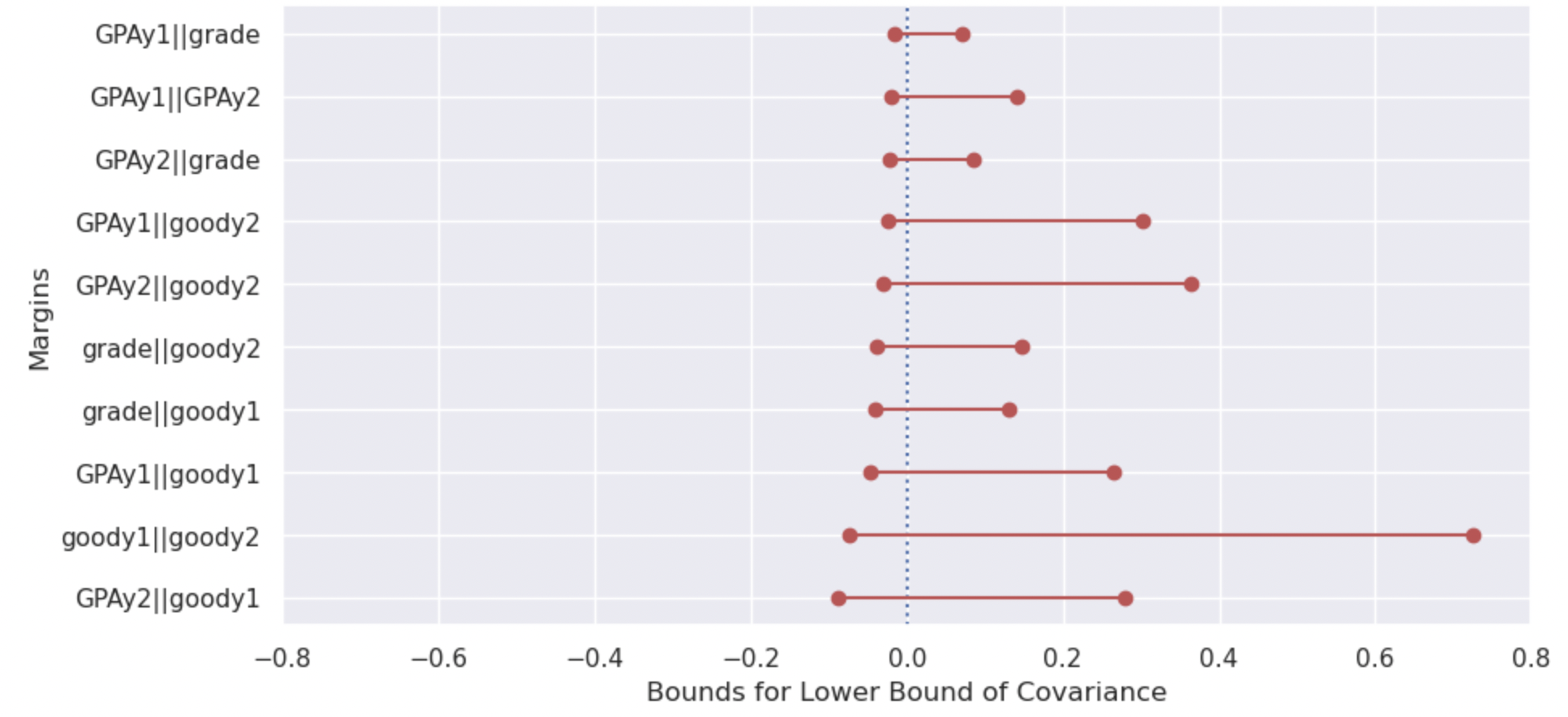
Figure 2: Lower and upper bounds for the covariance between different pairs of outcomes. Here GPAy1 means the GPA at the end of year 1, and similarly for GPAy2; goody1 means whether the student is in good standing at the end of year 1, and similarly for goody2; grade means the grade of the first semester in the first year.

4.4 Neymanian confidence interval

Continued from Example 2.3, we apply the proposed method to tighten the conventional estimator of the variance (5). We return to the Expitaxial layer growth dataset. In particular, we focus on the three treatment levels $(0,1)$, $(1,0)$, $(1,1)$ and consider the contrast $(Y_{i}(1,1)-Y_{i}(1,0)/2-Y_{i}(0,1)/2)$. Our lower bound of $S_{\tau}^{2}$ in (5) is noticeably greater than zero, indicating that bounding it by zero is overly conservative. As a result, our estimated variance has decreased the conventional counterpart by a significant $8.16$ percent. For sample size calculation, a reduction of $8.16$ percent in variance equates to a saving of $8.16$ percent in the number of units/repeats required. The results are shown in Table 3.

Table 3: Neymanina confidence intervals. The contrast effect estimate is $0.0533$.

Method	Variance estimate	95% Confidence interval for $\tau_{N}$
Convention	0.113	$(-0.609,0.711)$
Our proposal	0.104	$(-0.581,0.684)$

5 Discussion

In this work, we advocate for using MOT to obtain identified sets for causal estimands that are only partially identifiable. We perform theoretical analysis of the plug-in estimator of the identified sets, provide off-the-shelf implementation, and demonstrate the potentials of the approach for various causal tasks across multiple datasets.

We provide several future research directions.

• Covariate-assisted MOT. In the presence of covariates $X$, the conditional marginal distributions $Y(k)\mid X$ should be respected, a more stringent condition compared to preserving unconditional marginal distributions. We denote the set of joint couplings that adhere to these conditional marginals as $\Gamma_{X}$, then $\Gamma_{X}\subseteq\Gamma$ and yields larger population lower bounds of the objectives (3) and (2) with $\Gamma$ replaced by $\Gamma_{X}$. For empirical lower bound, conditioning on more covariates will decrease the estimation accuracy of the plug-in estimator. Striking a balance between the population’s lower bound and the empirical performance by selecting a subset of covariates and solving the associated MOT problem is of interest.

• Approximate joint mixability. For any $K$ centered distributions $\mu(1),...,\mu(K)$ on $\mathbb{R}^{d}$, they are jointly mixable if there exists a coupling such that for any $\bm{Y}(\cdot)$ on the support of the coupling, $\sum_{k=1}^{K}Y(k)/K=0$ [44]. The objective in Eq. (3) can be used to define a generalization of the joint mixability, where the level of joint mixability is evaluated by the 2-norm. One interesting phenomenon as an implication of Lemma C.2 is that the 2-norm approximate joint-mixability implies approximate joint-mixability in infinity norm for discretely supported distributions. Concretely, for any $\bm{Y}(\cdot)$ on the support of the optimal coupling in terms of objective in Eq.(3), we have $|\sum_{k=1}^{K}Y(k)/K|\lesssim 1/\sqrt{K}$ almost surely. This posits a promising research direction of approximate joint mixability. Many open problems can be considered, e.g., can we extend Lemma C.2 to arbitrary distributions? What are the relationships between the $p$-norm approximate joint mixability for $p\geq 1$?

• Implementation. There is a tradeoff between precision and the run time/resources. Especially when the accuracy tolerance $\varepsilon$ is small, the algorithm might become unstable due to floating point errors. Also, the run time will be much higher. Compared to OT, MOT requires a higher resolution, or equivalently a smaller tolerance parameter $\varepsilon$, due to a larger number (exponential to the number of margins) of cell probabilities, making the acceleration of even higher importance.

  Future work could explore potential ways to achieve higher precision in a more efficient way. One possibility is utilizing a low-rank tensor approximation to the quadratic objective function. In addition, in the current implementation, we use greedy Sinkhorn where the parameters are updated every $K$ iterations (after we calculate all $K$ margins). We have seen numerical success in simply updating one margin per iteration in a round-robin fashion, which is computationally economic. However, the convergence of this algorithm remains to be studied.

Appendix A Technical Lemma

Throughout the appendix, for any $L>0$, let $\mathcal{F}_{\mathrm{Lip},L}$ denote the $L$-Lipschitz function class supported on $B_{1}^{d}(0)$ such that all functions $\phi\in\mathcal{F}_{\mathrm{Lip},L}$ has $\phi(0)=0$. Denote by $\gamma^{\star}_{A}(\mu(1),\dots,\mu(K))$ the optimal coupling between $\mu(1),\dots,\mu(K)$ in terms of the objective Eq. (2). Denote by $\gamma^{\star}(\mu(1),\dots,\mu(K))$ the optimal coupling between $\mu(1),\dots,\mu(K)$ in terms of the objective Eq. (3).

Lemma A.1.

For any $\mu$ supported on $B_{1}^{d}(0)$, the Radermacher complexity of $\mathcal{F}_{L}$ under $\mu$ is bounded by

$$\mathcal{R}_{n}(\mathcal{F}_{L},\mu)\vcentcolon=\mathbb{E}_{\epsilon,X}\left[\sup_{\phi\in\mathcal{F}_{L}}\left\lvert\frac{1}{n}\sum_{i=1}^{n}\epsilon_{i}\phi(Y_{i})\right\rvert\right]\lesssim\begin{cases}Ln^{-2/d}&\text{if~{}}d>4,\\ Ln^{-1/2}\log n&\text{if~{}}d=4,\\ Ln^{-1/2}&\text{if~{}}d<4,\end{cases}$$

where $\epsilon=(\epsilon_{1},...\epsilon_{n})$, $\epsilon_{1},...,\epsilon_{n}$ are independent Radermacher variables and $Y_{1},...,Y_{n}$ are independent random variables sampled from the distribution $\mu$.

Proof of Lemma A.1.  We follow the derivation of [8, Lemma 4]. On $B_{1}^{d}(0)$, any function $\phi\in\mathcal{F}_{L}$ is bounded by $\|\phi\|_{\infty}\lesssim L$. Thus by [43, Theorem 5.22], we have

$$\mathcal{R}_{n}(\mathcal{F}_{L},\mu)\lesssim\inf_{\delta>0}\left(\delta+n^{-1/2}\int_{\delta}^{L}\sqrt{\log\mathcal{N}(\mathcal{F}_{L},\|\cdot\|_{\infty},u)du}\right),$$

where $\mathcal{N}(\mathcal{F}_{L},\|\cdot\|_{\infty},u)$ denotes the covering number of $\mathcal{F}_{L}$ in $\|\cdot\|_{\infty}$ at scale $u$. Then by [16, Theorem 1] which obtains $\log\mathcal{N}(\mathcal{F}_{L},\|\cdot\|_{\infty},u)\lesssim(u/L)^{-d/2}$, we have

$$\mathcal{R}_{n}(\mathcal{F}_{L},\mu) \lesssim\inf_{\delta>0}\left(\delta+n^{-1/2}\int_{\delta}^{L}(u/L)^{-d/4}du\right)$$

$$=\inf_{\delta>0}\left(\delta+Ln^{-1/2}\int_{\delta/L}^{1}u^{-d/4}du\right)$$

$$\lesssim\begin{cases}Ln^{-2/d}&\text{if~{}}d>4,\\ Ln^{-1/2}\log n&\text{if~{}}d=4,\\ Ln^{-1/2}&\text{if~{}}d<4,\end{cases}$$

where for $d<4$, we choose $\delta=0$ and $\delta=Ln^{-1/2}$ for $d=4$ and $\delta=Ln^{-2/d}$ for $d>4$. ∎

Lemma A.2.

For any $\mu$ supported on $B_{1}^{d}(0)$ and $\hat{\mu}_{n}$ an empirical distribution of $n$ independent samples, we have

$$\mathbb{E}\left[\sup_{\phi\in\mathcal{F}_{L}}\left\lvert\int\phi(y)d({\hat{\mu}}_{n}-\mu)\right\rvert\right]\lesssim 2\mathcal{R}_{n}(\mathcal{F}_{L},\mu)+Ln^{-1/2}.$$

Proof of Lemma A.2.  By [43, Theorem 4.10], we have for all $\delta>0$, with probability at least $1-\exp(-n\delta^{2}/(2L^{2}))$,

$$\sup_{\phi\in\mathcal{F}_{L}}\left\lvert\int\phi(y)d({\hat{\mu}}_{n}-\mu)\right\rvert\leq 2\mathcal{R}_{n}(\mathcal{F}_{L},\mu)+\delta.$$

Then since $\mathbb{E}[X]=\int_{0}^{\infty}\mathbb{P}(X\geq\delta)\textnormal{d}\delta$ for all positive random variable, we have

$$\mathbb{E}\left[\sup_{\phi\in\mathcal{F}_{L}}\left\lvert\int\phi(y)d({\hat{\mu}}_{n}-\mu)\right\rvert-2\mathcal{R}_{n}(\mathcal{F}_{L},\mu)\right]$$

$$\leq\mathbb{E}\left[\left(\sup_{\phi\in\mathcal{F}_{L}}\left\lvert\int\phi(y)d({\hat{\mu}}_{n}-\mu)\right\rvert-2\mathcal{R}_{n}(\mathcal{F}_{L},\mu)\right)_{+}\right]$$

$$=\int_{0}^{\infty}\mathbb{P}\left(\left(\sup_{\phi\in\mathcal{F}_{L}}\left\lvert\int\phi(y)d({\hat{\mu}}_{n}-\mu)\right\rvert-2\mathcal{R}_{n}(\mathcal{F}_{L},\mu)\right)_{+}\geq\delta\right)\textnormal{d}\delta$$

$$\leq\int_{0}^{\infty}\exp(-n\delta^{2}/(2L^{2}))\textnormal{d}\delta$$

$$\lesssim Ln^{-1/2}.$$

∎

Appendix B Omitted Proofs from Section 2

Lemma B.1.

For any $K$ distributions $\mu(1),\dots,\mu(K)$ on $\mathbb{R}^{d}$, let $\bar{\mu}(1),\dots,\bar{\mu}(K)$ be the centered counterpart, that is, $\bar{\mu}(k)$ is a translation of $\mu(k)$ by $-\mathbb{E}_{\mu(k)}\left[X\right]$ and $Y_{1}(k)\sim\mu(k)$ for $k\in[K]$. Then we have

$$\mathrm{MW}_{2}^{2}(\mu(1),\dots,\mu(K))=\mathrm{MW}_{2}^{2}(\bar{\mu}(1),\dots,\bar{\mu}(K))+\left\|\frac{\sum_{k=1}^{K}\mathbb{E}_{\mu(k)}[Y_{1}(k)]}{K}\right\|_{2}^{2}$$

Proof of Lemma B.1. 

Suppose $\gamma^{\star}=\gamma^{\star}(\mu(1),...,\mu(K))$ achieves $\mathrm{MW}_{2}^{2}(\mu(1),\dots,\mu(K))$, then we have

$$\mathrm{MW}_{2}^{2}(\mu(1),\dots,\mu(K))$$

$$=\int_{y}\left\|\frac{\sum_{k=1}^{K}y(k)}{K}\right\|^{2}\gamma^{\star}(dy)$$

$$=\int_{y}\left\|\frac{\sum_{k=1}^{K}\left(y(k)-\mathbb{E}_{\mu(k)}\left[Y_{1}(k)\right]\right)}{K}\right\|^{2}\gamma^{\star}(dy)+\left\|\frac{\sum_{k=1}^{K}\mathbb{E}_{\mu(k)}\left[Y_{1}(k)\right]}{K}\right\|_{2}^{2}$$

$$\leq\mathrm{MW}_{2}^{2}(\bar{\mu}(1),\dots,\bar{\mu}(K))+\left\|\frac{\sum_{k=1}^{K}\mathbb{E}_{\mu(k)}\left[Y_{1}(k)\right]}{K}\right\|_{2}^{2}.$$

The inequality can be reversed considering the optimal coupling $\bar{\gamma}^{\star}=\gamma^{\star}(\bar{\mu}(1),...,\bar{\mu}(K))$, which concludes our proof. ∎

Lemma B.2.

For any $K$ distributions $\mu(1),\dots,\mu(K)$ on $\mathbb{R}^{d}$, let $\bar{\mu}(1),\dots,\bar{\mu}(K)$ be the centered counterpart, that is, $\bar{\mu}(k)$ is a translation of $\mu(k)$ by $-\mathbb{E}_{\mu(k)}\left[X\right]$ and $Y_{1}(k)\sim\mu(k)$ for $k\in[K]$. Let $A$ be any symmetric matrix. Then we have

$$\mathrm{QMW}(\mu(1),\dots,\mu(K);A)=\mathrm{QMW}(\bar{\mu}(1),\dots,\bar{\mu}(K);A)+\sum_{k,l}a_{kl}\left\langle\mathbb{E}_{\mu(k)}[Y_{1}(k)],\mathbb{E}_{\mu(l)}[Y_{1}(l)]\right\rangle.$$

Proof of Lemma B.2.  Suppose $\gamma^{\star}=\gamma^{\star}(\mu(1),...,\mu(K);A)$ achieves $\mathrm{QMW}(\mu(1),...,\mu(K);A)$, then we have

$$\mathrm{QMW}(\mu(1),\dots,\mu(K);A)$$

$$=\int_{y}\sum_{k,l}a_{kl}\left\langle y(k),y(l)\right\rangle\gamma^{\star}(dy)$$

$$=\int_{y}\sum_{k,l}a_{kl}\left\langle y(k)-\mathbb{E}_{\mu(k)}[Y_{1}(k)],y(l)-\mathbb{E}_{\mu(l)}[Y_{1}(l)]\right\rangle\gamma^{\star}(dy)+\sum_{k,l}a_{kl}\left\langle\mathbb{E}_{\mu(k)}[Y_{1}(k)],\mathbb{E}_{\mu(l)}[Y_{1}(l)]\right\rangle$$

$$\leq\mathrm{QMW}(\bar{\mu}(1),\dots,\bar{\mu}(K);A)+\sum_{k,l}a_{kl}\left\langle\mathbb{E}_{\mu(k)}[Y_{1}(k)],\mathbb{E}_{\mu(l)}[Y_{1}(l)]\right\rangle.$$

The inequality can be reversed considering the optimal coupling $\bar{\gamma}^{\star}=\gamma^{\star}(\bar{\mu}(1),...,\bar{\mu}(K))$, which concludes our proof. ∎

Appendix C Omitted Proofs from Section 3

C.1 Upper bound

Lemma C.1.

For any matrix $A=(a_{ij})_{1\leq i,j\leq K}$, we have

$$\mathbb{E}\left[\left\lvert\sum_{k,l}a_{kl}\left\langle\mathbb{E}_{\mu_{\star}(k)}Y_{1}(k),\mathbb{E}_{\mu_{\star}(l)}Y_{1}(l)\right\rangle-\sum_{k,l}a_{kl}\left\langle\mathbb{E}_{\hat{\mu}_{n}(k)}Y_{1}(k),\mathbb{E}_{\hat{\mu}_{n}(l)}Y_{1}(l)\right\rangle\right\rvert\right]\lesssim K\sqrt{\sum_{k,l}a_{kl}^{2}}\cdot n^{-1/2}.$$

Proof of Lemma C.1.  We first separate the quantity

$$\sum_{k,l}a_{kl}\left\langle\mathbb{E}_{\mu_{\star}(k)}Y_{1}(k),\mathbb{E}_{\mu_{\star}(l)}Y_{1}(l)\right\rangle-\sum_{k,l}a_{kl}\left\langle\mathbb{E}_{\hat{\mu}_{n}(k)}Y_{1}(k),\mathbb{E}_{\hat{\mu}_{n}(l)}Y_{1}(l)\right\rangle$$

$$=\sum_{k=1}^{K}a_{kk}\left(\left\langle\mathbb{E}_{\mu_{\star}(k)}[Y_{1}(k)],\mathbb{E}_{\mu_{\star}(k)}[Y_{1}(k)]\right\rangle-\left\langle\mathbb{E}_{\hat{\mu}(k)}[Y_{1}(k)],\mathbb{E}_{\hat{\mu}(k)}[Y_{1}(k)]\right\rangle\right)$$

$$\quad+\sum_{k\neq l}a_{kl}\left\langle\mathbb{E}_{\mu_{\star}(k)}[Y_{1}(k)],\mathbb{E}_{\mu_{\star}(l)}[Y_{1}(l)]\right\rangle$$

$$\quad-\sum_{k\neq l}a_{kl}\left\langle\mathbb{E}_{\hat{\mu}_{n}(k)}[Y_{1}(k)],\mathbb{E}_{\hat{\mu}_{n}(l)}[Y_{1}(l)]\right\rangle$$

$$=\sum_{k=1}^{K}a_{kk}\left\langle\mathbb{E}_{\mu_{\star}(k)}Y_{1}(k)-\mathbb{E}_{\hat{\mu}_{n}(k)}Y_{1}(k),\mathbb{E}_{\mu_{\star}(k)}Y_{1}(k)+\mathbb{E}_{\hat{\mu}_{n}(k)}Y_{1}(k)\right\rangle$$

$$\quad+\sum_{k\neq l}a_{kl}\left\langle\mathbb{E}_{\mu_{\star}(k)}[Y_{1}(k)],\mathbb{E}_{\mu_{\star}(l)-\hat{\mu}_{n}(l)}[Y_{1}(l)]\right\rangle$$

$$\quad+\sum_{k\neq l}a_{kl}\left\langle\mathbb{E}_{\mu_{\star}(k)-\hat{\mu}_{n}(k)}[Y_{1}(k)],\mathbb{E}_{\hat{\mu}_{n}(l)}[Y_{1}(l)]\right\rangle.$$

Then, by triangle inequality together with Khintchine’s inequality (Exercise 2.6.7 of [42]), we have

$$\mathbb{E}\left[\left\lvert\sum_{k,l}a_{kl}\left\langle\mathbb{E}_{\mu_{\star}(k)}Y_{1}(k),\mathbb{E}_{\mu_{\star}(l)}Y_{1}(l)\right\rangle-\sum_{k,l}a_{kl}\left\langle\mathbb{E}_{\hat{\mu}_{n}(k)}Y_{1}(k),\mathbb{E}_{\hat{\mu}_{n}(l)}Y_{1}(l)\right\rangle\right\rvert\right]$$

$$\leq\mathbb{E}\left[\left\lvert\sum_{k=1}^{K}a_{kk}\left\langle\mathbb{E}_{\mu_{\star}(k)}Y_{1}(k)-\mathbb{E}_{\hat{\mu}_{n}(k)}Y_{1}(k),\mathbb{E}_{\mu_{\star}(k)}Y_{1}(k)+\mathbb{E}_{\hat{\mu}_{n}(k)}Y_{1}(k)\right\rangle\right\rvert\right]$$

$$\quad+\sum_{k=1}^{K}\mathbb{E}\left[\mathbb{E}_{\mu_{\star}(k)}\left\lvert\mathbb{E}_{(\mu_{\star}-\hat{\mu}_{n})(-k)}\left[\sum_{l\neq k}a_{kl}\left\langle Y_{1}(k),Y_{1}(l)\right\rangle\right]\right\rvert\right]$$

$$\quad+\sum_{k=1}^{K}\mathbb{E}\left[\mathbb{E}_{\hat{\mu}_{n}(k)}\left\lvert\mathbb{E}_{(\mu_{\star}-\hat{\mu}_{n})(-k)}\left[\sum_{l\neq k}a_{kl}\left\langle Y_{1}(k),Y_{1}(l)\right\rangle\right]\right\rvert\right]$$

$$\lesssim\left(\sqrt{\sum_{k=1}^{K}a_{kk}^{2}}+\sum_{k=1}^{K}\sqrt{\sum_{l\neq k}a_{kl}^{2}}\right)(n/K)^{-1/2}$$

$$\lesssim\sqrt{K\cdot\sum_{k,l}a_{kl}^{2}}\cdot(n/K)^{-1/2},$$

where the last inequality is by Cauchy-Shwartz. ∎

Proposition C.1.

For any symmetric matrix $A\in\mathbb{R}^{K\times K}$, we have

$$\begin{split}&\mathbb{E}\left[\left|\mathrm{QMW}(\hat{\mu}_{n}(1),\dots\hat{\mu}_{n}(K);A)-\mathrm{QMW}(\mu_{\star}(1),\dots,\mu_{\star}(K);A)\right|\right]\\ &\lesssim K\sqrt{\sum\limits_{k=1}^{K}a_{kk}^{2}}\cdot n^{-1/2}+\left(\sum\limits_{k=1}^{K}|a_{kk}|\right)\wedge\begin{cases}\eta_{K,d,A}\cdot K^{3/2}(n/K)^{-2/d},&\text{if }d>4,\\ \eta_{K,d,A}\cdot K^{2}n^{-1/2}\log(n/K),&\text{if }d=4,\\ \eta_{K,d,A}\cdot K^{2}n^{-1/2},&\text{if }d<4,\end{cases}\end{split}$$ (8)

where the notation $\lesssim$ hides constants that only depend on the dimension $d$. Moreover, the coefficient $\eta_{K,d,A}$ is defined as

$$\eta_{K,d,A}\vcentcolon=\sup_{\begin{subarray}{c}\mu(1),\dots,\mu(K)\\ \text{with zero mean}\end{subarray}}\hskip 3.0pt\sup_{\begin{subarray}{c}(y(1),\dots,y(K))\in\\ \mathrm{supp}\left(\gamma^{\star}_{A}(\mu(1),\dots,\mu(K))\right)\end{subarray}}\sup_{k\in[K]}\left\|\sum\limits_{l\neq k}\frac{a_{kl}y(l)}{\sqrt{K}}\right\|,$$

where $\mu(1),\dots,\mu(K)$ are $d$-dimensional distributions with zero mean and $(y(1),\dots,y(K))$ in the support of the coupling $\gamma^{\star}_{A}(\mu(1),\dots,\mu(K))$.

Proof of Proposition C.1.  By lemmas B.2 and C.1, we know that the objective can be separated and the mean of the coupling concentrates. Thus, without loss of generality, in this proof, we only consider the marginals $\mu_{\star}(1),\dots,\mu_{\star}(K),\hat{\mu}_{n}(1),\dots,\hat{\mu}_{n}(K)$ that have zero means. For any $K$ marginals $\mu(1),\dots,\mu(K)$ supported on $B_{1}^{d}(0)\subset\mathbb{R}^{d}$, we have

$$\mathrm{QMW}(\mu(1),\dots,\mu(K);A)$$

$$\vcentcolon=\inf_{\gamma\in\Gamma(\mu(1),\dots,\mu(K))}\int\sum\limits_{i,j}a_{ij}y(i)^{\top}y(j)~{}\gamma(dy)$$

$$\leq\sum\limits_{k=1}^{K}a_{kk}\int\|y(k)\|^{2}\mu(k,dy(k))+\sum\limits_{i\neq j}a_{ij}\int y(i)^{\top}y(j)~{}\mu(i,dy(i))\mu(j,dy(j))$$

$$=\sum\limits_{k=1}^{K}a_{kk}\int\|y(k)\|^{2}\mu(k,dy(k))\leq\sum\limits_{k=1}^{K}|a_{kk}|,$$

where the first inequality is by choosing the independent coupling $\gamma(dy)=\prod_{k=1}^{K}\mu(k,dy(k))$ and the last inequality is by the boundedness of $y$. This implies

$$\left\lvert\mathrm{QMW}(\mu_{\star}(1),\dots,\mu_{\star}(K);A)-\mathrm{QMW}(\hat{\mu}_{n}(1),\dots,\hat{\mu}_{n}(K);A)\right\rvert\leq\sum\limits_{k=1}^{K}|a_{kk}|.$$ (9)

Now by the classic duality of [23], we have

$$\mathrm{QMW}(\mu(1),\dots,\mu(K);A)=\sup_{\begin{subarray}{c}f_{1},\dots,f_{K}:\\ \sum\limits_{k=1}^{K}f_{k}(y(k))\leq y^{\top}Ay\end{subarray}}\sum\limits_{k=1}^{K}\int f_{k}(y(k))\mu(k,dy(k)),$$

where $\mu(k,dy(k))$ denote the marignal distribution of $\mu(k)$ on $y(k)$. We first separate the square terms out, since they only concern one marginal as

$$\sup_{\begin{subarray}{c}f_{1},\dots,f_{K}:\\ \sum\limits_{k=1}^{K}f_{k}(y(k))\leq y^{\top}Ay\end{subarray}}\sum\limits_{k=1}^{K}\int f_{k}(y(k))\mu(k,dy(k))$$

$$=\sum\limits_{k=1}^{K}\int a_{kk}\|y(k)\|^{2}\mu(k,dy(k))+\sup_{\begin{subarray}{c}f_{1},\dots,f_{K}:\\ \sum\limits_{k=1}^{K}f_{k}(y(k))\leq y^{\top}Ay\end{subarray}}\sum\limits_{k=1}^{K}\int f_{k}(y(k))-a_{kk}\|y(k)\|^{2}\mu(k,dy(k))$$

$$=\sum\limits_{k=1}^{K}\int a_{kk}\|y(k)\|^{2}\mu(k,dy(k))+\sup_{\begin{subarray}{c}\phi_{1},\dots,\phi_{K}:\\ \sum\limits_{k=1}^{K}\phi_{k}(y(k))\leq\sum\limits_{i\neq j}a_{ij}y^{\top}(i)y(j)\end{subarray}}\sum\limits_{k=1}^{K}\int\phi_{k}(y(k))\mu(k,dy(k)),$$ (10)

where the second equality is by setting $\phi_{k}(y(k))=f_{k}(y(k))-a_{kk}\|y(k)\|^{2}$. Now we are going to show that there exists a sequence of supremum achieving functions $\phi^{\star}_{1},\dots,\phi^{\star}_{K}$ that all lie in the space of $\mathcal{F}_{\mathrm{Lip},2K}$. To start with, we note again by the classical duality of [23] that there exists $\widetilde{\phi}_{1},\dots,\widetilde{\phi}_{K}$ that achieves the supremum in eq. 10. For $k=1,\dots,K$, we iteratively define the function $\phi^{\star}_{k}$ as

$$\phi^{\star}_{k}(y)\vcentcolon=\inf_{\begin{subarray}{c}y(1),\dots,y(K)\\ \in\mathrm{supp}(\gamma^{\star}_{A}(\mu(1),\dots,\mu(K)))\end{subarray}}2\left\langle y,\sum\limits_{l\neq k}a_{kl}y(l)\right\rangle+\sum\limits_{\begin{subarray}{c}i,j:i\neq j,\\ i\neq k,j\neq k\end{subarray}}a_{ij}\langle y(i),y(j)\rangle-\sum_{l=1}^{k-1}\phi^{\star}_{l}(y(l))-\sum_{l=k+1}^{K}\widetilde{\phi}_{l}(y(l)).$$

And prove by induction that $\phi^{\star}_{1},\dots,\phi^{\star}_{k},\widetilde{\phi}_{k+1},\dots,\widetilde{\phi}_{K}$ are admissible and achieve the supremum in eq. 10. When $k=0$, the claim is true by definition. Now suppose the claim is true up to $k-1$. For any $k$, by definition, we have for any $y(1),\dots,y(K)$

$$\sum_{l=1}^{k}\phi^{\star}_{l}(y(l))+\sum_{l=k+1}^{K}\widetilde{\phi}_{l}(y(l))\leq\sum\limits_{i\neq j}a_{ij}y(i)y(j).$$

Thus $\phi^{\star}_{1},\dots,\phi^{\star}_{k},\widetilde{\phi}_{k+1},\dots,\widetilde{\phi}_{K}$ are admissible function for the supremum in eq. 10. Furthermore, by the induction hypothesis, $\phi^{\star}_{1},\dots,\phi^{\star}_{k-1},\widetilde{\phi}_{k},\dots,\widetilde{\phi}_{K}$ are admissible function and achieves the supremum in eq. 10, we have for any $y(1),\dots,y(k)$

$$\sum_{l=1}^{k-1}\phi^{\star}_{l}(y(l))+\sum_{l=k}^{K}\widetilde{\phi}_{l}(y(l))\leq\sum\limits_{i\neq j}a_{ij}y(i)y(j).$$

This implies

$$2\left\langle y(k),\sum\limits_{l\neq k}a_{kl}y(l)\right\rangle+\sum\limits_{\begin{subarray}{c}i,j:i\neq j,\\ i\neq k,j\neq k\end{subarray}}a_{ij}\langle y(i),y(j)\rangle-\sum_{l=1}^{k-1}\phi^{\star}_{l}(y(l))-\sum_{l=k+1}^{K}\widetilde{\phi}_{l}(y(l))\geq\widetilde{\phi}_{k}(y(k)).$$

Then take infimum over $y(1),\dots,y(k-1),y(k+1),\dots,y(K)$, we have

$$\phi^{\star}_{k}(y(k))\geq\widetilde{\phi}_{k}(y(k)).$$

This implies that $\phi^{\star}_{1},\dots,\phi^{\star}_{k},\widetilde{\phi}_{k+1},\dots,\widetilde{\phi}_{K}$ achieves the supremum in eq. 10. Thus by induction, we have shown that $\phi^{\star}_{1},\dots,\phi^{\star}_{K}$ are admissible function and achieves the supremum in eq. 10. Furthermore, since for any $k$, $\phi_{k}$ are infimum of linear functions, the Lipschitz constant for $\phi_{k}$ is thus upper bounded by

$$\sup_{\begin{subarray}{c}y(1),\dots,y(k-1),\\ y(k+1),\dots,y(K)\\ \in\mathrm{supp}(\gamma^{\star}_{A}(\mu(1),\dots,\mu(K)))\end{subarray}}2\left\|\sum\limits_{l\neq k}a_{kl}y(l)\right\|\leq 2\eta_{K,d,A}\sqrt{K}.$$

Therefore,

$$\mathrm{QMW}(\hat{\mu}_{n}(1),\dots\hat{\mu}_{n}(1);A)-\mathrm{QMW}(\mu_{\star}(1),\dots,\mu_{\star}(K);A)$$

$$=\sum\limits_{k=1}^{K}\int a_{kk}\|y(k)\|^{2}\left(\hat{\mu}_{n}(k,dy(k))-\mu_{\star}(k,dy(k))\right)$$

$$\quad\quad+\sup_{\begin{subarray}{c}\phi_{1},\dots,\phi_{K}:\\ \sum\limits_{k=1}^{K}\phi_{k}(y(k))\leq\sum\limits_{i\neq j}a_{ij}y^{\top}(i)y(j)\\ \phi_{k}:2\sqrt{K}\eta_{K,d,A}\text{-Lip.}\end{subarray}}\sum\limits_{k=1}^{K}\int\phi_{k}(y(k))\hat{\mu}_{n}(k,dy(k))$$

$$\quad\quad-\sup_{\begin{subarray}{c}\phi_{1},\dots,\phi_{K}:\\ \sum\limits_{k=1}^{K}\phi_{k}(y(k))\leq\sum\limits_{i\neq j}a_{ij}y^{\top}(i)y(j)\\ \phi_{k}:2\sqrt{K}\eta_{K,d,A}\text{-Lip.}\end{subarray}}\sum\limits_{k=1}^{K}\int\phi_{k}(y(k))\mu_{\star}(k,dy(k))$$

$$\leq\sum\limits_{k=1}^{K}\int a_{kk}\|y(k)\|^{2}\left(\hat{\mu}_{n}(k,dy(k))-\mu_{\star}(k,dy(k))\right)$$

$$\quad\quad+\sup_{\begin{subarray}{c}\phi_{1},\dots,\phi_{K}:\\ \sum\limits_{k=1}^{K}\phi_{k}(y(k))\leq\sum\limits_{i\neq j}a_{ij}y^{\top}(i)y(j)\\ \phi_{k}:2\sqrt{K}\eta_{K,d,A}\text{-Lip.}\end{subarray}}\sum\limits_{k=1}^{K}\int\phi_{k}(y(k))(\hat{\mu}_{n}(k,dy(k))-\mu_{\star}(k,dy(k)))$$

$$\leq\left\lvert\sum\limits_{k=1}^{K}\int a_{kk}\|y(k)\|^{2}\left(\hat{\mu}_{n}(k,dy(k))-\mu_{\star}(k,dy(k))\right)\right\rvert$$

$$\quad\quad+\sum\limits_{k=1}^{K}\sup_{\phi_{k}\in\mathcal{F}_{\mathrm{Lip},2\sqrt{K}\eta_{K,d,A}}}\int\phi_{k}(y(k))\left(\hat{\mu}_{n}(k,dy(k))-\mu_{\star}(k,dy(k))\right).$$

Similarly we can show $-(\mathrm{QMW}(\hat{\mu}_{n}(1),\dots\hat{\mu}_{n}(1);A)-\mathrm{QMW}(\mu_{\star}(1),\dots,\mu_{\star}(K);A))$ satisfies the same upper bound. By Hoeffding’s inequality (Proposition 2.5 of [43]), we have

$$\mathbb{E}\left\lvert\sum\limits_{k=1}^{K}\int a_{kk}\|y(k)\|^{2}\left(\hat{\mu}_{n}(k,dy(k))-\mu_{\star}(k,dy(k))\right)\right\rvert\lesssim\left(\sum\limits_{k=1}^{K}|a_{kk}|\right)\cdot(n/K)^{-1/2}.$$ (11)

Finally, by Lemma A.2, we obtain

$$\begin{split}\hskip 144.54pt&\mathbb{E}\left[\sum\limits_{k=1}^{K}\sup_{\phi_{k}\in\mathcal{F}_{\mathrm{Lip},2\sqrt{K}\eta_{K,d,A}}}\int\phi_{k}(y(k))\left(\hat{\mu}_{n}(k,dy(k))-\mu_{\star}(k,dy(k))\right)\right]\\ &\lesssim K^{3/2}\eta_{K,d,A}\cdot\begin{cases}(n/K)^{-2/d},&\text{if }d>4,\\ (n/K)^{-1/2}\log(n/K),&\text{if }d=4,\\ (n/K)^{-1/2},&\text{if }d<4,\end{cases}.\end{split}$$ (12)

The bound from eq. 11 is lower order compared to the bound of the mean concentration from lemma C.1. In all, combine Lemma C.1, eq. 9, and eq. 12, we have

$$\begin{split}&\mathbb{E}\left[\left|\mathrm{QMW}(\hat{\mu}_{n}(1),\dots\hat{\mu}_{n}(K);A)-\mathrm{QMW}(\mu_{\star}(1),\dots,\mu_{\star}(K);A)\right|\right]\\ &\lesssim K\sqrt{\sum\limits_{k=1}^{K}a_{kk}^{2}}\cdot n^{-1/2}+\left(\sum\limits_{k=1}^{K}|a_{kk}|\right)\wedge\begin{cases}\eta_{K,d,A}\cdot K^{3/2}(n/K)^{-2/d},&\text{if }d>4,\\ \eta_{K,d,A}\cdot K^{2}n^{-1/2}\log(n/K),&\text{if }d=4,\\ \eta_{K,d,A}\cdot K^{2}n^{-1/2},&\text{if }d<4,\end{cases}\end{split}$$

∎

Lemma C.2.

For $n,K\geq 2$ and $d\geq 1$, for any $K$ mean zero marginals $\mu(1),\dots,\mu(K)$ finitely supported on $B_{1}^{d}(0)\subset\mathbb{R}^{d}$, we have

$$\sup_{\begin{subarray}{c}(y(1),\dots,y(K))\in\\ \mathrm{supp}\left(\gamma^{\star}(\mu(1),\dots,\mu(K))\right)\end{subarray}}\sup_{l\in[K]}\left\|\sum\limits_{k\neq l}\frac{y(k)}{\sqrt{K}}\right\|\leq 4.$$

$(y(1),\dots,y(K))$ in the support of the optimal coupling $\gamma^{\star}(\mu(1),\dots,\mu(K))$ with respect to the objective in Eq. (3).

Proof of Lemma C.2.  Denote the set $\mathcal{A}_{1}=\left\{y:\left\|\sum\limits_{k=1}^{K}y(k)\right\|\leq 2\sqrt{K}\right\}$ and $\mathcal{A}_{2}=\left\{y:\left\|\sum\limits_{k=1}^{K}y(k)\right\|\geq 4\sqrt{K}-1\right\}$. We prove by contradition. Suppose otherwise, then we have $\gamma^{\star}(\mathcal{A}_{2})>0$. On the other hand, we note that the objective value is upper bounded by

$$\mathrm{MW}_{2}^{2}(\mu(1),\dots,\mu(K)) =\int\left\|\frac{\sum_{k=1}^{K}y(k)}{K}\right\|_{2}^{2}\gamma^{\star}(dy)$$

$$\leq\int\left\|\frac{\sum_{k=1}^{K}y(k)}{K}\right\|_{2}^{2}\prod_{k=1}^{K}\mu(k,dy(k)),$$

$$=\frac{1}{K^{2}}\sum\limits_{k=1}^{K}\int\|y(k)\|^{2}\mu(k,dy(k))\leq\frac{1}{K}.$$

Then by Markov’s inequality, we have $\gamma^{\star}(\mathcal{A}_{1})>3/4$. Since all the marginals are finitely supported, we can find $y_{1}\in\mathcal{A}_{1}$ and $y_{2}\in\mathcal{A}_{2}$ such that $\gamma^{\star}(y_{1}),\gamma^{\star}(y_{2})>0$. Let $p=\gamma^{\star}(y_{1})\wedge\gamma^{\star}(y_{2})$. For any $j,k\in[K]$, we consider $y_{1,j}(k)=(y_{1}(1),\dots,y_{1}(j-1),y_{2}(j),y_{1}(j+1),\dots,y_{1}(K))$ and $y_{2,j}(k)=(y_{2}(1),\dots,y_{2}(j-1),y_{1}(j),y_{2}(j+1),\dots,y_{2}(K))$. Then since the $K$ couplings $\gamma^{\star}-p(\delta_{y_{1}}+\delta_{y_{2}})+p(\delta_{y_{1,j}}+\delta_{y_{2,j}})$ for $j\in[K]$ are no better than the optimal coupling in the objective value, we thus have for $j\in[K]$,

$$\left\|\sum\limits_{k=1}^{K}y_{1}(k)\right\|^{2}+\left\|\sum\limits_{k=1}^{K}y_{2}(k)\right\|^{2}\leq\left\|y_{2}(j)+\sum_{k\neq j}y_{1}(k)\right\|^{2}+\left\|y_{1}(j)+\sum_{k\neq j}y_{2}(k)\right\|^{2}.$$

Simplifying the expression, we obtain for any $j\in[K]$,

$$\left\langle y_{1}(j)-y_{2}(j),\sum\limits_{k\neq j}(y_{1}(k)-y_{2}(k))\right\rangle\leq 0.$$

This further implies

$$\left\langle y_{1}(j)-y_{2}(j),\sum\limits_{k}(y_{1}(k)-y_{2}(k))\right\rangle\leq\|y_{1}(j)-y_{2}(j)\|^{2}.$$

Summing up over $j\in[K]$, we have

$$\left\|\sum\limits_{k}(y_{1}(k)-y_{2}(k))\right\|^{2}\leq\sum\limits_{k=1}^{K}\left\|(y_{1}(k)-y_{2}(k))\right\|^{2}\leq 2K.$$

However, we have

$$4\sqrt{K}-1\leq\left\|\sum\limits_{k=1}^{K}y_{2}(k)\right\|\leq\left\|\sum\limits_{k=1}^{K}y_{1}(k)\right\|+\left\|\sum\limits_{k=1}^{K}(y_{1}(k)-y_{2}(k))\right\|\leq(2+\sqrt{2})\sqrt{K}.$$

This is a contradiction. Thus have $\gamma^{\star}(\mathcal{A}_{2})=0$, which means

$$\sup_{\begin{subarray}{c}(y(1),\dots,y(K))\in\\ \mathrm{supp}\left(\gamma^{\star}(\mu(1),\dots,\mu(K))\right)\end{subarray}}\sup_{k\in[K]}\left\|\sum\limits_{l\neq k}\frac{y(l)}{\sqrt{K}}\right\|\leq 4.$$

∎

Lemma C.3 (Theorem 7.7 of [34]; [39]).

Suppose $P$ and $Q$ are two distributions on the space $\mathcal{X}$. Provided that the diagonal $\{(x,x):x\in\mathcal{X}\}$ is measurable.

$${\sf TV}(P,Q)=\min_{P_{X,Y}}\{P_{X,Y}[X\neq Y]:P_{X}=P,P_{Y}=Q\}$$

where minimization is over the coupling distributions $P_{X,Y}$ with that $P_{X}=P$ and $P_{Y}=Q$.

Proof of Theorem 3.1. 

By applying proposition C.1 with $A=\mathbbm{1}\mathbbm{1}^{\top}/K^{2}$, we first obtain the following convergence rate: For any $n,d,K$, we have

$$\begin{split}\hskip 144.54pt&\mathbb{E}\left[\left|\mathrm{MW}_{2}^{2}(\hat{\mu}_{n}(1),\dots\hat{\mu}_{n}(K))-\mathrm{MW}_{2}^{2}(\mu_{\star}(1),\dots,\mu_{\star}(K))\right|\right]\\ &\lesssim n^{-1/2}+\left(1/K\right)\wedge\begin{cases}\eta_{K,d}\cdot K^{-1/2}(n/K)^{-2/d},&\text{if }d>4,\\ \eta_{K,d}\cdot n^{-1/2}\log(n/K),&\text{if }d=4,\\ \eta_{K,d}\cdot n^{-1/2},&\text{if }d<4,\end{cases}\end{split}$$ (13)

where the notation $\lesssim$ hides constants that only depend on the dimension $d$. Moreover, the coefficient $\eta_{K,d}$ is defined as

$$\eta_{K,d}\vcentcolon=\sup_{\begin{subarray}{c}\mu(1),\dots,\mu(K)\\ \text{with zero mean}\end{subarray}}\hskip 3.0pt\sup_{\begin{subarray}{c}(y(1),\dots,y(K))\in\\ \mathrm{supp}\left(\gamma^{\star}(\mu(1),\dots,\mu(K))\right)\end{subarray}}\sup_{l\in[K]}\left\|\sum\limits_{k\neq l}\frac{y(k)}{\sqrt{K}}\right\|,$$

where $\mu(1),\dots,\mu(K)$ are $d$-dimensional distributions with zero mean and $(y(1),\dots,y(K))$ in the support of the optimal coupling $\gamma^{\star}(\mu(1),\dots,\mu(K))$ with respect to the objective in Eq. (3). Moreover, since the support is bounded, we have, $\eta_{K,d}\leq\frac{K-1}{\sqrt{K}}\leq\sqrt{K}$. Let $N\geq n$ be an integer to be specified later. Let $\hat{\mu}_{N}=(\hat{\mu}_{N}(1),\dots,\hat{\mu}_{N}(K))$ be the emprical distribution sampled from $\mu_{\star}$ where each margin has $N/K$ samples. Then eq. 13 implies

$$\begin{split}\hskip 144.54pt&\mathbb{E}\left[\left|\mathrm{MW}_{2}^{2}(\hat{\mu}_{N}(1),\dots\hat{\mu}_{N}(K))-\mathrm{MW}_{2}^{2}(\mu_{\star}(1),\dots,\mu_{\star}(K))\right|\right]\\ &\lesssim N^{-1/2}+\left(1/K\right)\wedge\begin{cases}(N/K)^{-2/d},&\text{if }d>4,\\ (N/K)^{-1/2}\log(N/K),&\text{if }d=4,\\ (N/K)^{-1/2},&\text{if }d<4.\end{cases}\end{split}$$

Let $\bar{\mu}_{n}=(\bar{\mu}_{n}(1),\dots,\bar{\mu}_{n}(K))$. The distribution $\bar{\mu}_{n}$ is the empirical distribution sampled from $\hat{\mu}_{N}$ with replacement where each margin has $n/K$ samples. Since $\hat{\mu}_{N}$ and $\bar{\mu}_{n}$ are both discretely supported, then rerun the proof of proposition C.1 with lemma C.2 gives the following convergence rate due to improved Lipschitz constant

$$\begin{split}\hskip 144.54pt&\mathbb{E}_{\hat{\mu}_{N},\bar{\mu}_{n}}\left[\left|\mathrm{MW}_{2}^{2}(\bar{\mu}_{n}(1),\dots,\bar{\mu}_{n}(K))-\mathrm{MW}_{2}^{2}(\hat{\mu}_{N}(1),\dots\hat{\mu}_{N}(K))\right|\right]\\ &\lesssim n^{-1/2}+\left(1/K\right)\wedge\begin{cases}K^{-1/2}(n/K)^{-2/d},&\text{if }d>4,\\ n^{-1/2}\log(n/K),&\text{if }d=4,\\ n^{-1/2},&\text{if }d<4,\end{cases}\end{split}$$

Finally, we consider the variables $\widetilde{\mu}_{n}=(\widetilde{\mu}_{n}(1),\dots,\widetilde{\mu}_{n}(K))$, which is the emprical distribution sampled from $\hat{\mu}_{N}$ without replacement where each margin has $n/K$ samples. We couple $\widetilde{\mu}_{n}$ and $\bar{\mu}_{n}$ conditioned on $\hat{\mu}_{N}$ by the ${\sf TV}$ distance achieving coupling $P_{\widetilde{\mu}_{n},\bar{\mu}_{n}}$ as defined in lemma C.3. Thus in all, we have

$$\mathbb{E}_{\hat{\mu}_{n}}\left[\left|\mathrm{MW}_{2}^{2}(\hat{\mu}_{n}(1),\dots\hat{\mu}_{n}(K))-\mathrm{MW}_{2}^{2}(\mu_{\star}(1),\dots,\mu_{\star}(K))\right|\right]$$

$$=\mathbb{E}_{\widetilde{\mu}_{n}}\left[\left|\mathrm{MW}_{2}^{2}(\widetilde{\mu}_{n}(1),\dots\widetilde{\mu}_{n}(K))-\mathrm{MW}_{2}^{2}(\mu_{\star}(1),\dots,\mu_{\star}(K))\right|\right]$$

$$\leq\mathbb{E}_{\hat{\mu}_{N},\widetilde{\mu}_{n},\bar{\mu}_{n}}\left[\left|\mathrm{MW}_{2}^{2}(\hat{\mu}_{N}(1),\dots\hat{\mu}_{N}(K))-\mathrm{MW}_{2}^{2}(\mu_{\star}(1),\dots,\mu_{\star}(K))\right|\right]$$

$$\quad+\mathbb{E}_{\hat{\mu}_{N},\widetilde{\mu}_{n},\bar{\mu}_{n}}\left[\left|\mathrm{MW}_{2}^{2}(\hat{\mu}_{N}(1),\dots\hat{\mu}_{N}(K))-\mathrm{MW}_{2}^{2}(\bar{\mu}_{n}(1),\dots,\bar{\mu}_{n}(K))\right|\right]$$

$$\quad+\mathbb{E}_{\hat{\mu}_{N},\widetilde{\mu}_{n},\bar{\mu}_{n}}\left[\left|\mathrm{MW}_{2}^{2}(\bar{\mu}_{n}(1),\dots,\bar{\mu}_{n}(K))-\mathrm{MW}_{2}^{2}(\widetilde{\mu}_{n}(1),\dots\widetilde{\mu}_{n}(K))\right|\right]$$

$$\lesssim{\sf TV}(\bar{\mu}_{n},\widetilde{\mu}_{n})+N^{-1/2}+n^{-1/2}+\begin{cases}(N/K)^{-2/d}+K^{-1/2}(n/K)^{-2/d},&\text{if }d>4,\\ (N/K)^{-1/2}\log(N/K)+n^{-1/2}\log(n/K),&\text{if }d=4,\\ (N/K)^{-1/2}+n^{-1/2},&\text{if }d<4,\end{cases}$$

where the first equality is due to the fact that $\hat{\mu}_{n}$ and $\widetilde{\mu}_{n}$ is equal in distribution, the second inequality is by triangle inequality and the third inequality is by combing the aforementioned rates. Now we finally show ${\sf TV}(\bar{\mu}_{n},\widetilde{\mu}_{n})$ is $o(1)$ as $N\to\infty$ and then take $N\to\infty$ to obtain the desired result. Concretely, let event $\mathcal{E}_{N,n,K}=\{\text{no points in $\hat{\mu}_{N}$ are sampled twice when sampling $\bar{\mu}_{n}$ with replacement}\}$. Then we have $\bar{\mu}_{n}|\mathcal{E}_{N,n,K}=\widetilde{\mu}_{n}$. Thus,

$${\sf TV}(\bar{\mu}_{n},\widetilde{\mu}_{n})\leq 1-\mathbb{P}_{\bar{\mu}_{n}}(\mathcal{E}_{N,n,K})=o(1),\quad\text{as }N\to\infty.$$

This concludes our proof.

∎

Proof of Proposition 3.1.  This is a direct corollary of proposition C.1, by the upper bound of

$$\eta_{K,d,A}\lesssim\left\|A\right\|_{1,\infty}/\sqrt{K}.$$

∎

C.2 Lower bound

Remark C.1.

Consider a pathological case: $X_{i}(1/K)\sim\mathcal{N}(0,(K-1)^{2})$, $X_{i}(m/K)\sim\mathcal{N}(0,1)$, in this way,

$$MW_{2}^{2}(\mu_{n}^{1:K})=\left(\frac{\sum_{i=1}^{n}y_{i}}{n}\right)^{2}=O(1),\quad MW_{2}^{2}(\mu^{1:K})\sim 0.$$

Therefore, the gap $MW_{2}^{2}(\mu_{n}^{1:K})-MW_{2}^{2}(\mu^{1:K})$ is of order $O(1)$ despite the sample size $n$. However, the random variales are not bounded. Also the response is not Lipschitz.

Proof of LABEL:lemm:lower.bound.  On one hand, the asymptotic result of the squared 2-Wasserstein’s distance for $d=1$,

$$\sqrt{n}\left(W_{2}^{2}({\mu}_{n}^{1},{\mu}_{n}^{2})-W_{2}^{2}({\mu}^{1},{\mu}^{2})\right)\stackrel{{\scriptstyle d}}{{\to}}\mathcal{N}(0,\sigma^{2}),\quad\sigma^{2}>0,~{}\mu^{1}\neq\mu^{2},$$

suggesting that the upper bound is likely to be sharp for $d\leq 4$. On the other hand, for $d>4$, let $\mu^{1}=U([0,1]^{d})$, $\mu^{2}=U([0,1]^{d})+\bm{c}$, $\bm{c}\in\mathbb{R}^{d}$. We use $\mu_{n}^{1}$, $\mu_{n}^{2}$, $\mu_{n}^{{}^{\prime}1}$ to denote the empirical distribution of $\bm{X}_{i}\sim\mu^{1}$, $\bm{Y}_{i}\sim\mu^{2}$, $\bm{Y}_{i}-c\sim\mu^{1}$, $i\in[n]$, where $(\bm{X}_{i})\mathchoice{\mathrel{\hbox to0.0pt{$\displaystyle\perp$\hss}\mkern 2.0mu{\displaystyle\perp}}}{\mathrel{\hbox to0.0pt{$\textstyle\perp$\hss}\mkern 2.0mu{\textstyle\perp}}}{\mathrel{\hbox to0.0pt{$\scriptstyle\perp$\hss}\mkern 2.0mu{\scriptstyle\perp}}}{\mathrel{\hbox to0.0pt{$\scriptscriptstyle\perp$\hss}\mkern 2.0mu{\scriptscriptstyle\perp}}}(\bm{Y}_{i})$. Then

$$W_{2}^{2}(\mu^{1},\mu^{2})=\|c\|_{2}^{2},\quad W_{2}^{2}(\mu_{n}^{1},\mu_{n}^{2})=W_{2}^{2}(\mu_{n}^{1},\mu_{n}^{{}^{\prime}1})+\|c\|_{2}^{2},\implies W_{2}^{2}(\mu_{n}^{1},\mu_{n}^{2})-W_{2}^{2}(\mu^{1},\mu^{2})=W_{2}^{2}(\mu_{n}^{1},\mu_{n}^{{}^{\prime}1})\gtrsim n^{-2/d}.$$

∎

Proof of Proposition 3.2.  We only need to prove for $d=1$. For any $K\geq 2$, if $K$ is even, then consider $\mu(1)=\dots=\mu(K)=Ber(1/2)$ and $\mu^{\prime}(1)=\dots=\mu^{\prime}(K)=Ber(1/2+\varepsilon)$ with some $\varepsilon>0$ to be decided later. If $K$ is odd, then set the $\mu(K)=\mu^{\prime}(K)$ to be the point mass distribution on $0$ and we reduce back to the even case. We first show that $\mathrm{MW}_{2}^{2}(\mu(1),\dots,\mu(K))=1/4$ and $\mathrm{MW}_{2}^{2}(\mu^{\prime}(1),\dots,\mu^{\prime}(K))\geq 1/4+\varepsilon$. Indeed, by Lemma B.1, we have

$$\mathrm{MW}_{2}^{2}(\mu(1),\dots,\mu(K))\geq\left(\frac{\sum_{k=1}^{K}\mathbb{E}_{\mu(k)}[X]}{K}\right)^{2}=1/4$$

and

$$\mathrm{MW}_{2}^{2}(\mu^{\prime}(1),\dots,\mu^{\prime}(K))\geq\left(\frac{\sum_{k=1}^{K}\mathbb{E}_{\mu(k)}[X]}{K}\right)^{2}\geq 1/4+\varepsilon.$$

Meanwhile, for $\mu(1),\dots,\mu(K)$ the coupling $\gamma$ that assigns $Y(1)=Y(3)=\dots=Y(K-1)$ and $Y(2)=Y(4)=\dots=Y(K)=1-Y(1)$ is an admissible coupling that achieves

$$\int\left(\sum\limits_{k=1}^{K}y(K)/K\right)^{2}\gamma(dy)=1/4.$$

Thus we have shown $\mathrm{MW}_{2}^{2}(\mu(1),\dots,\mu(K))=1/4$ and $\mathrm{MW}_{2}^{2}(\mu^{\prime}(1),\dots,\mu^{\prime}(K))\geq 1/4+\varepsilon$. Let $\mathbb{P}$ be the distribution on the observations $Y_{i}(1),\dots,Y_{i}(K)$ with $\mu_{\star}(1),\dots,\mu_{\star}(K)=\mu(1),\dots,\mu(K)$ and $\mathbb{P}^{\prime}$ be the distribution on the observations $Y_{i}(1),\dots,Y_{i}(K)$ with $\mu_{\star}(1),\dots,\mu_{\star}(K)=\mu^{\prime}(1),\dots,\mu^{\prime}(K)$. Then we have

$${\sf TV}(\mathbb{P},\mathbb{P}^{\prime})\lesssim\sqrt{\mathrm{KL}(\mathbb{P},\mathbb{P}^{\prime})}\lesssim\sqrt{n\cdot\mathrm{KL}(Ber(1/2),Ber(1/2+\varepsilon))}\lesssim\sqrt{n\varepsilon^{2}}.$$

Thus by choosing $\varepsilon=c\cdot n^{-1/2})$ for constant $c$ small enough, we can make ${\sf TV}(\mathbb{P},\mathbb{P}^{\prime})\leq 1/2$ while $\mathrm{MW}_{2}^{2}(\mu^{\prime}(1),\dots,\mu^{\prime}(K))-\mathrm{MW}_{2}^{2}(\mu(1),\dots,\mu(K))\gtrsim\Omega(n^{-1/2})$. Then we apply Le Cam’s two-point method (Lemma 1 of [48]) and obtain a lower bound of $n^{-1/2}$. Furthermore, since our problem has $K$ margins, it is easy to embed the 1-Wasserstein distance estimation problem in the first two margins. Thus, by the lower bound of Wasserstein distance estimation from theorem 22 of [29], we obtain a lower bound of $K^{-2}(n/K)^{-2/d}$ when $d>4$. ∎

Appendix D Algorithms from Section 4

In this section, we introduce the MOT Greenkhorn algorithm and MOT Sinkhorn algorithm that we implemented. We then specify the following three properties we use regarding the MOT Sinkhorn algorithm: (1) The convergence guarantee. (2) The application of log-exp-sum trick. (3) The lower bounds without convergence.

For any $\gamma$ a $K$-marginal tensor, define

$$\mathrm{MTV}(\gamma,\mu(1),\dots,\mu(K))\vcentcolon=\sum\limits_{k=1}^{K}\int_{y(k)}|\gamma(k,dy(k))-\mu(k,dy(k))|,$$

where $\gamma(k,dy(k))=\int_{y(1),...,y(k-1),y(k+1),...,y(K)}\gamma(dy(1),...,dy(K))$ which might be a signed measure in general.

Multi-marginal Greenkhorn

We follow [2] and introduce the algorithm of MOT Greenkhorn. The function $\rho(a,b)$ in Line 5 of Algorithm 1 is defined as $\rho(a,b)=b-a+a\log(a/b)$.

Algorithm 1 Multi-marginal Greenkhorn

1:Cost matrix $C$, Multiple marignals $\mu(1)$, $\mu(2)$, …,$\mu(K)$, Accuracy $\varepsilon>0$.

2:$\eta\leftarrow 4\sum\nolimits_{k=1}^{K}\log n_{k}/\varepsilon$, $\varepsilon^{\prime}\leftarrow\frac{\varepsilon}{8\|C\|_{\infty}}$, $A\leftarrow\exp(-\eta C)$.

3:$m(k)\leftarrow\mathbf{0}\in\mathbb{R}^{n_{k}}$ for $k\in[K]$, and $\gamma\leftarrow A/\|A\|_{1}$.

4:while $\mathrm{MTV}(\gamma,\mu(1),...,\mu(K)))>\varepsilon^{\prime}$ do

5:     $(k^{\star},i^{\star})\leftarrow\mathop{\mathrm{argmax}}_{k\in[K],i\in[n_{k}]}\rho(\mu(k,i),\gamma(k,i))$. $\triangleright$ $\mu(k,i)$ is $1/n_{k}$ in our case.

6:     $m(k^{\star},i^{\star})\leftarrow m(k^{\star},i^{\star})+\log\mu(k^{\star},i^{\star})-\log\gamma(k^{\star},i^{\star})$.

7:      $\gamma(i_{1},\dots,i_{K})=A(i_{1},\dots,i_{K})\cdot\prod_{k=1}^{K}\exp(m(k,i_{k}))$ for all $i_{1},\dots,i_{K}\in[n_{1}]\times\cdots\times[n_{K}]$.

8:end while

9:Let $\hat{\gamma}^{(0)}=\gamma$.

10:for $k=1,...,K$ do

11:     $v(k)\leftarrow(\mu(k)/\hat{\gamma}^{(k-1)}(k))\wedge\mathbbm{1}$, where the division and $\wedge$ are elementwise operation.

12:     $\hat{\gamma}^{(k)}(i_{1},\dots,i_{K})=\hat{\gamma}^{(k-1)}(i_{1},\dots,i_{K})\cdot v(k,i_{k})$ for all $i_{1},\dots,i_{K}\in[n_{1}]\times\cdots\times[n_{K}]$.

13:end for

14:for $k=1,...,K$ do

15:     $\mathrm{err}_{k}\leftarrow\mu(k)-\hat{\gamma}^{(K)}(k)$.

16:end for

17:return $\hat{\gamma}(i_{1},...,i_{K})\leftarrow\hat{\gamma}^{(K)}(i_{1},...,i_{K})+\prod_{k=1}^{K}\mathrm{err}_{k}(i_{k})/\|\mathrm{err}_{K}\|_{1}^{K-1}$ for all $i_{1},...,i_{K}$.

Multi-marginal Sinkhorn

We use the Multi-marginal Sinkhorn algorithm as in Algorithm 2 .

Algorithm 2 Multi-marginal Sinkhorn

1:Parameters: Cost tensor $C\in\mathbb{R}^{n_{1}\times\dots\times n_{k}}$, Marignals $\mu(1),\dots,\mu(K)$, Targeted accuracy $\varepsilon>0$.

2:Let $\eta=(4\sum_{k=1}^{K}\log n_{k})/\varepsilon$, $\varepsilon^{\prime}=\varepsilon/(8\|C\|_{\infty})$, and $A=\exp(-\eta C)$ .

3:Let $t=0$, $m^{(0)}(k)=\mathbf{0}\in\mathbb{R}^{n_{k}}$ for $k\in[K]$, and $\gamma^{(0)}=A/\|A\|_{1}$.

4:for $t=1,2,\dots$ do

5:     Let $k_{t}=\mathop{\mathrm{argmax}}_{k}\sum_{i_{k}\in[n_{k}]}\mu(k,i_{k})\log(\mu(k,i_{k})/\gamma^{(t-1)}(k,i_{k}))$.

6:     $m^{(t)}(k_{t})=m^{(t-1)}(k_{t})+\log\mu(k_{t})-\log\gamma^{(t-1)}(k_{t})$.

7:      $\gamma^{(t)}(i_{1},\dots,i_{K})=A(i_{1},\dots,i_{K})\cdot\prod_{l=1}^{k}\exp(m^{(t)}(l,i_{l}))\prod_{l=k+1}^{K}\exp(m^{(t-1)}(l,i_{l}))$ for all $i_{1},\dots,i_{K}\in[n_{1}]\times\cdots\times[n_{K}]$.

8:     if  $\mathrm{MTV}(\gamma^{(t)},\mu(1),\dots,\mu(K))\leq\varepsilon^{\prime}$  then break

9:end for

10:Let $\hat{\gamma}^{(0)}=\gamma^{(t)}$.

11:for $k=1,...,K$ do

12:     $v(k)\leftarrow(\mu(k)/\hat{\gamma}^{(k-1)}(k))\wedge\mathbbm{1}$, where the division and $\wedge$ are elementwise operation.

13:     $\hat{\gamma}^{(k)}(i_{1},\dots,i_{K})=\hat{\gamma}^{(k-1)}(i_{1},\dots,i_{K})\cdot v(k,i_{k})$ for all $i_{1},\dots,i_{K}\in[n_{1}]\times\cdots\times[n_{K}]$.

14:end for

15:for $k=1,...,K$ do

16:     $\mathrm{err}_{k}\leftarrow\mu(k)-\hat{\gamma}^{(K)}(k)$.

17:end for

18:return $\hat{\gamma}(i_{1},...,i_{K})\leftarrow\hat{\gamma}^{(K)}(i_{1},...,i_{K})+\prod_{k=1}^{K}\mathrm{err}_{k}(i_{k})/\|\mathrm{err}_{K}\|_{1}^{K-1}$ for all $i_{1},...,i_{K}$.

The guarantees that are interesting for us are shown in the following:

D.1 Convergence

Theorem D.1 (Theorem 16 of [27]).

When Algorithm 2 converges, we have

$$\inf_{\gamma\in\Gamma(\mu(1),...,\mu(K))}\int_{y}C(y)\gamma(dy)\geq\int_{y}C(y)\hat{\gamma}(dy)-\varepsilon.$$

D.2 Application of Log-Sum-Exp Trick

Log-sum-exp trick

Let $f:\mathcal{X}\to\mathbb{R}$ be any function with $\mathcal{X}$ being any finite set. The celebrated log-sum-exp trick is used for computing quantities of the type $\log\sum_{x\in\mathcal{X}}\exp(f(x))$. It computes the equivalent form of $\max_{x}f(x)+\log\sum_{x}\exp(f(x)-\max_{x^{\prime}}f(x^{\prime}))$, which is much more stable computationally since $\sum_{x}\exp(f(x)-\max_{x^{\prime}}f(x^{\prime}))\geq 1$ and $f(x)-\max_{x^{\prime}}f(x^{\prime})\leq 0$ for all $x\in\mathcal{X}$.

In the implementation of Algorithm 2, the log-sum-exp trick can be apply to compute the update of $m^{(t)}(k)$: For Algorithm 2 specifically, the computation in Line 7 is unstable when $\varepsilon$ is chosen small because it involves exponential to the power of magnitude $\Omega(\eta)=\Omega(1/\varepsilon)$. We can apply the celebrated log-sum-exp trick to stabilize the algorithm by skipping Line 7 and updating $m^{(t)}(k_{t})$ in Line 6 for the next timestep by

$$m^{(t)}(k_{t}) =m^{(t-1)}(k_{t})+\log\mu(k_{t})$$

$$-\log\sum\limits_{\begin{subarray}{c}i_{1},\dots,i_{k_{t}-1}\\ i_{k_{t}+1},\dots,i_{K}\end{subarray}}\exp\left(-\eta C(i_{1},\dots,i_{k_{t}-1},\cdot,i_{k_{t}+1},\dots,i_{K})+\sum\limits_{l\neq k_{t}}m^{(t-1)}(l,i_{l})\right),$$

where the final term is executed using the log-sum-exp trick.

D.3 Lower Bounds without Convergence

Lemma D.1 (Section 4.4 of [33]).

For any $t\geq 1$, Algorithm 2 satisfies

$$\inf_{\gamma\in\Gamma(\mu(1),...,\mu(K))}\int_{y}C(y)\gamma(dy)\geq\frac{1}{\eta}\sum_{k=1}^{K}\int_{y(k)}m^{(t)}(y(k))\mu(k,dy(k)).$$

References

- [1] Martial Agueh and Guillaume Carlier “Barycenters in the Wasserstein space” In SIAM Journal on Mathematical Analysis 43.2 SIAM, 2011, pp. 904–924
- [2] Jason Altschuler, Jonathan Niles-Weed and Philippe Rigollet “Near-linear time approximation algorithms for optimal transport via Sinkhorn iteration” In Advances in neural information processing systems 30, 2017
- [3] Jason Altschuler, Jonathan Weed and Philippe Rigollet “Near-linear time approximation algorithms for optimal transport via Sinkhorn iteration”, 2018 arXiv:1705.09634 [cs.DS]
- [4] Joshua Angrist, Daniel Lang and Philip Oreopoulos “Incentives and services for college achievement: Evidence from a randomized trial” In American Economic Journal: Applied Economics 1.1 American Economic Association, 2009, pp. 136–163
- [5] Peter M Aronow, Donald P Green and Donald KK Lee “Sharp bounds on the variance in randomized experiments” In The Annals of Statistics 42.3 Institute of Mathematical Statistics, 2014, pp. 850–871
- [6] Peter J Bickel et al. “Efficient and adaptive estimation for semiparametric models” Springer, 1993
- [7] M. P. Bitler, J. B. Gelbach and H. W. Hoynes “Can Variation in Subgroups’ Average Treatment Effects Explain Treatment Effect Heterogeneity? Evidence from a Social Experiment” Working Paper, 2010 URL: http://www.socsci.uci.edu/~mbitler/papers/bgh-subgroups-paper.pdf
- [8] Lenaic Chizat et al. “Faster wasserstein distance estimation with the sinkhorn divergence” In Advances in Neural Information Processing Systems 33, 2020, pp. 2257–2269
- [9] Yunjey Choi et al. “Stargan: Unified generative adversarial networks for multi-domain image-to-image translation” In Proceedings of the IEEE conference on computer vision and pattern recognition, 2018, pp. 8789–8797
- [10] Marco Cuturi “Sinkhorn Distances: Lightspeed Computation of Optimal Transportation Distances”, 2013 arXiv:1306.0895 [stat.ML]
- [11] Simone Di Marino, Augusto Gerolin and Luca Nenna “Optimal transportation theory with repulsive costs” In Topological optimization and optimal transport 17, 2015, pp. 204–256
- [12] Yanqin Fan and Sang Soo Park “Sharp bounds on the distribution of treatment effects and their statistical inference” In Econometric Theory 26.3 Cambridge University Press, 2010, pp. 931–951
- [13] Rémi Flamary et al. “Pot: Python optimal transport” In Journal of Machine Learning Research 22.78, 2021, pp. 1–8
- [14] Maurice Fréchet “Sur les tableaux de corrélation dont les marges sont données” In Annals University Lyon: Series A 14, 1951, pp. 53–77
- [15] Alfred Galichon “Optimal transport methods in economics” Princeton University Press, 2018
- [16] Adityanand Guntuboyina and Bodhisattva Sen “L1 covering numbers for uniformly bounded convex functions” In Conference on Learning Theory, 2012, pp. 12–1 JMLR WorkshopConference Proceedings
- [17] James J Heckman, Jeffrey Smith and Nancy Clements In The Review of Economic Studies 64.4 Wiley-Blackwell, 1997, pp. 487–535
- [18] Le Hui et al. “Unsupervised multi-domain image translation with domain-specific encoders/decoders” In 2018 24th International Conference on Pattern Recognition (ICPR), 2018, pp. 2044–2049 IEEE
- [19] Shayan Hundrieser, Thomas Staudt and Axel Munk “Empirical optimal transport between different measures adapts to lower complexity” In arXiv preprint arXiv:2202.10434, 2022
- [20] Guido W Imbens and Donald B Rubin “Causal inference in statistics, social, and biomedical sciences” Cambridge university press, 2015
- [21] Albert Jacquard “Heritability: one word, three concepts” In Biometrics JSTOR, 1983, pp. 465–477
- [22] Tingyan Jia “Empathy, Motivated Reasoning, And Redistribution”, 2022
- [23] Hans G Kellerer “Duality theorems for marginal problems” In Zeitschrift für Wahrscheinlichkeitstheorie und verwandte Gebiete 67 Springer, 1984, pp. 399–432
- [24] Brendan Kline and Elie Tamer “Recent developments in partial identification” In Annual Review of Economics 15 Annual Reviews, 2023, pp. 125–150
- [25] Mark J Laan and James M Robins “Unified methods for censored longitudinal data and causality” Springer, 2003
- [26] Tianyi Lin, Nhat Ho and Michael Jordan “On efficient optimal transport: An analysis of greedy and accelerated mirror descent algorithms” In International Conference on Machine Learning, 2019, pp. 3982–3991 PMLR
- [27] Tianyi Lin, Nhat Ho, Marco Cuturi and Michael I Jordan “On the complexity of approximating multimarginal optimal transport” In The Journal of Machine Learning Research 23.1 JMLRORG, 2022, pp. 2835–2877
- [28] Jiannan Lu “On randomization-based and regression-based inferences for 2k factorial designs” In Statistics & Probability Letters 112 Elsevier, 2016, pp. 72–78
- [29] Tudor Manole and Jonathan Niles-Weed “Sharp convergence rates for empirical optimal transport with smooth costs” In The Annals of Applied Probability 34.1B Institute of Mathematical Statistics, 2024, pp. 1108–1135
- [30] Charles F Manski “The mixing problem in programme evaluation” In The Review of Economic Studies 64.4 Wiley-Blackwell, 1997, pp. 537–553
- [31] Roger B Nelsen “An introduction to copulas” Springer, 2006
- [32] Brendan Pass “Multi-marginal optimal transport: theory and applications” In ESAIM: Mathematical Modelling and Numerical Analysis 49.6, 2015, pp. 1771–1790
- [33] Gabriel Peyré and Marco Cuturi “Computational optimal transport: With applications to data science” In Foundations and Trends® in Machine Learning 11.5-6 Now Publishers, Inc., 2019, pp. 355–607
- [34] Yury Polyanskiy and Yihong Wu “Information Theory: From Coding to Learning” In Cambridge University Press, 2022+ URL: https://people.lids.mit.edu/yp/homepage/data/itbook-export.pdf
- [35] Donald B Rubin “Estimating causal effects of treatments in randomized and nonrandomized studies” In Journal of Educational Psychology 66.5 American Psychological Association, 1974, pp. 688–701
- [36] Ludger Rüschendorf “Mathematical risk analysis” In Springer Ser. Oper. Res. Financ. Eng. Springer, Heidelberg Springer, 2013
- [37] Jerzy Splawa-Neyman “On the application of probability theory to agricultural experiments. Essay on principles. Section 9.” In Statistical Science JSTOR, 1923, pp. 465–472
- [38] Thomas Staudt and Shayan Hundrieser “Convergence of Empirical Optimal Transport in Unbounded Settings” In arXiv preprint arXiv:2306.11499, 2023
- [39] Volker Strassen “The existence of probability measures with given marginals” In The Annals of Mathematical Statistics 36.2 Institute of Mathematical Statistics, 1965, pp. 423–439
- [40] Nazarii Tupitsa, Pavel Dvurechensky, Alexander Gasnikov and César A Uribe “Multimarginal optimal transport by accelerated alternating minimization” In 2020 59th ieee conference on decision and control (cdc), 2020, pp. 6132–6137 IEEE
- [41] Aad W Vaart “Asymptotic statistics” Cambridge university press, 2000
- [42] Roman Vershynin “High-dimensional probability: An introduction with applications in data science” Cambridge university press, 2018
- [43] Martin J Wainwright “High-dimensional statistics: A non-asymptotic viewpoint” Cambridge university press, 2019
- [44] Bin Wang and Ruodu Wang “Joint mixability” In Mathematics of Operations Research 41.3 INFORMS, 2016, pp. 808–826
- [45] Ruodu Wang, Liang Peng and Jingping Yang “Bounds for the sum of dependent risks and worst Value-at-Risk with monotone marginal densities” In Finance and Stochastics 17.2 Springer, 2013, pp. 395–417
- [46] CF Jeff Wu and Michael S Hamada “Experiments: planning, analysis, and optimization” John Wiley & Sons, 2011
- [47] Yujia Xie, Xiangfeng Wang, Ruijia Wang and Hongyuan Zha “A fast proximal point method for computing exact wasserstein distance” In Uncertainty in artificial intelligence, 2020, pp. 433–453 PMLR
- [48] Bin Yu “Assouad, fano, and le cam” In Festschrift for Lucien Le Cam: research papers in probability and statistics Springer, 1997, pp. 423–435