Learning dynamical behaviors in physical systems
Abstract
Physical learning is an emerging paradigm in science and engineering whereby (meta)materials acquire desired macroscopic behaviors by exposure to examples. So far, it has been applied to static properties such as elastic moduli and self-assembled structures encoded in minima of an energy landscape. Here, we extend this paradigm to dynamic functionalities, such as motion and shape change, that are instead encoded in limit cycles or pathways of a dynamical system. We identify the two ingredients needed to learn time-dependent behaviors irrespective of experimental platforms: (i) learning rules with time delays and (ii) exposure to examples that break time-reversal symmetry during training. After providing a hands-on demonstration of these requirements using programmable LEGO toys, we turn to realistic particle-based simulations where the training rules are not programmed on a computer. Instead, we elucidate how they emerge from physico-chemical processes involving the causal propagation of fields, like in recent experiments on moving oil droplets with chemotactic signalling. Our trainable particles can self-assemble into structures that move or change shape on demand, either by retrieving the dynamic behavior previously seen during training, or by learning on the fly. This rich phenomenology is captured by a modified Hopfield spin model amenable to analytical treatment. The principles illustrated here provide a step towards von Neumann’s dream of engineering synthetic living systems that adapt to the environment.
Biological systems adapt to their environment by changing their behavior in response to past events: once bitten, twice shy. In the brain, for instance, neurons wire together (i.e. increase their interactions) if they fire together. But the ability to learn is not limited to sentient or animate beings: it can emerge in natural physical processes in which interactions increase between entities that happen to be correlated, a paradigm known as Hebbian learning [1, 1]. Inanimate systems too can evolve their microscopic interactions to effectively learn desired behaviors after experiencing examples of that behavior, a phenomenon often referred to as physical learning [2, 3, 4]. So far, physical learning has been applied to static behaviors, such as elastic responses or self-assembled shapes and particles configurations characteristic of equilibrium systems [5, 6, 7, 8, 9, 10, 11, 12, 9, 13, 14, 15, 10, 16, 17]. Such static targets are encoded in fixed points, i.e. local minima of an energy landscape.
In this article, we ask: how can a physical system learn time-dependent functionalities like pathways, trajectories, or dynamic states such as limit cycles? The essence of our approach is conceptualized schematically in Fig. 1: an external operator first imposes a dynamic state, that breaks time-reversal symmetry, on the system during a period called training (e.g. moves the wings of the origami bird in Fig. 1a). Next, during a period that we call retrieval, the desired time-dependent state (e.g. wings flapping) can be recovered as the system evolves according to asymmetric microscopic interactions learned during training (Fig. 1b).
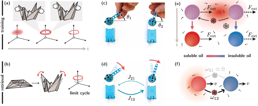
Our foundational step is to identify the basic ingredients needed to learn dynamical states irrespective of experimental platforms. We begin with a hands-on demonstration of these requirements using the programmable LEGO toy shown in Fig. 1c-d and Movie 1. The toy has two angular degrees of freedom and that can be controlled by hand very much like the angles of the origami-bird wings. These angles follow a dynamics enabled by sensors and actuators where each angle tends to align or antialign with the other depending on the tunable couplings and (here represents the effect of on ). During the training phase, the operator changes the angles by hand over time. The time series of the angles are in turn mapped into distinct values of the couplings by a learning rule programmed on a computer. The simplest Hebbian learning rule, in which increases when and are simultaneously aligned, precludes dynamic states because only symmetric interactions () are learned. In order to retrieve dynamic states (Fig. 1d), asymmetric couplings () are generically needed [28, 29, 30, 31, 32, 33, 34, 35, 36, 37, 38, 39, 40, 41, 42, 43, 44, 45, 46, 47, 48, 49, 50].
Asymmetric couplings can be learned if a time delay is added in the learning rule (Movie 1). For instance, we can impose that tends to increase when is correlated with . This creates the desired asymmetry between and . But it is not enough: the system must be trained using examples that break time-reversal symmetry, in order for the asymmetry not to be washed out over time (see Movie 1). Learning rules with signal-propagation delays naturally arise from causality and are reminiscent of spike-timing-dependent plasticity (STDP) in neuroscience [51, 52, 53, 54, 55, 56]: the influence of neuron on neuron increases if fires just before fires (but not if fires just after ).
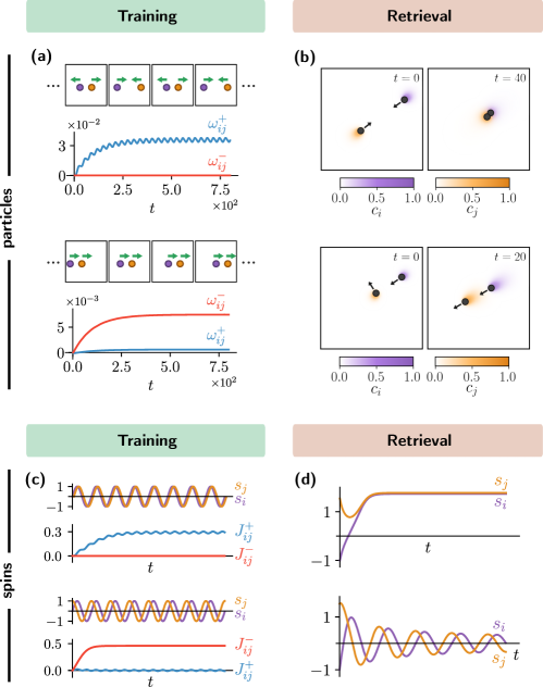
Learning time-dependent states in physical systems.—In the example of Fig. 1c-d, a computer is needed to program the dynamics of the system during both training and retrieval. We now demonstrate our approach in situations where the learning rule capable of learning non-reciprocal interactions is not programmed on a computer, but instead naturally emerge from basic physico-chemical processes. Figure 1e-f shows an example of trainable interaction between oil droplets [18, 19, 20, 22, 23, 24, 25, 26, 27, 57]. The droplets are composed of a mixture of two chemicals: the red oil can easily be solubilized in water, while the blue one is less soluble. It has been observed experimentally that this asymmetry in their composition can lead to a motion of the droplets in which the red droplet chases the blue one [18].
The aforementioned process is what we need in our proposal of a concrete training protocol for learning time-dependent states in droplets experiments. In the training phase, forces are applied on two droplets with identical initial composition (purple in panel e). When the droplets move fast enough (i.e. at large enough Péclet number, see caption and next section), the asymmetric diffusion of the red miscible oil due to the motion of the droplets (see the comet-like diffusion cloud in top part of panel e) leads to a change in their composition (bottom part of panel e). Crucially, the red oil of the front droplet can be captured by the back droplet, but not vice-versa. As a consequence, the droplets tend to reproduce the motion seen in training during the retrieval phase where they are left to freely evolve (panel f). We refer the reader to Methods for more detailed experimental considerations.
The key feature of the example of Fig. 1e-f is the appearance of time-delayed interactions arising from the combination of the particles’ motion during training with the causal propagation of signals through a field (e.g., oil concentration in Fig. 1). Beyond this specific example, all physical interactions are subject to retarded potentials due to causality, for example asymmetric forces between acoustically levitated particles or hydrodynamic interactions mediated by the wakes of objects moving in a fluid [47]. We now consider a simplified particle-based model that captures this ubiquitous feature in a minimal mathematical setting amenable to analytic treatment.
Particles with field-mediated interactions.—Consider particles at positions (Fig. 2a) that are sources for distinct fields (e.g. chemicals such as different types of oil with distinct solubilities as in Fig. 1e-f) with concentration (shown in yellow in Fig. 2a). These concentration fields evolve according to
| (1) |
The first term describes the emission of with rate in a circle of radius around particle ( is the Heaviside function). The second and third terms describe respectively decay at rate and diffusion with diffusion constant .
The positions of the particles follow the overdamped dynamics
| (2) |
with steric repulsion , translational noise , and self-propulsion with speed and a direction set by the (generalized) mobilities , that describe the tendency of particle to move along gradients of . The could be, for example, chemotactic or diffusiophoretic mobilities whose values are fixed at the end of the training phase (see Methods for detailed modelling, e.g. the influence of angular inertia).
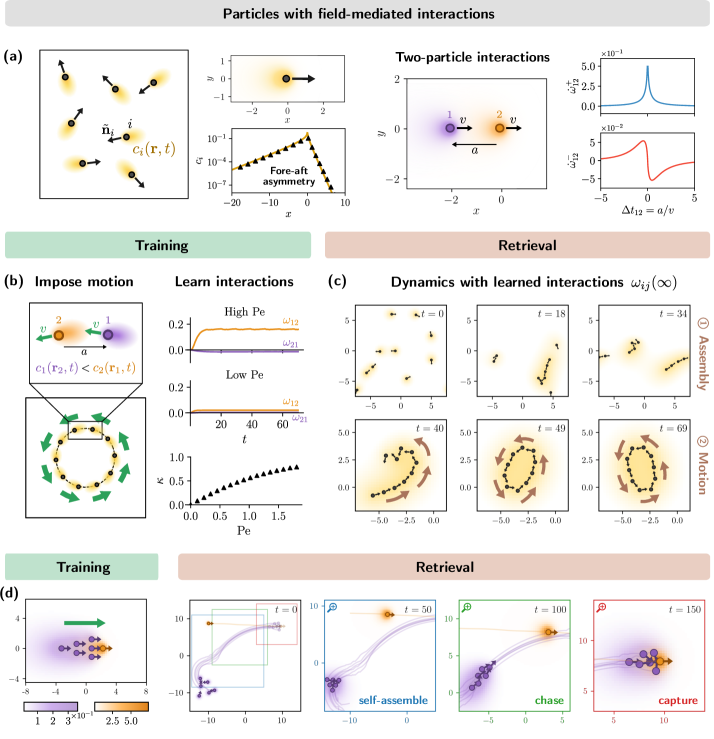
Inspired by the experimental proposal in Fig. 1e-f, we formulate the following training rule that captures mathematically how the evolve as a function of the trajectories that the operator imposes by hand during training (overruling Eq. (2)):
| (3) |
Here is the learning rate and is a relaxation time. In a nutshell, this learning rule increases the mobility when particle detects a greater-than-average value of . In addition to the mechanism sketched in Fig. 1, such strengthening of interactions based on spatial co-localization of chemical species or other constituents can be achieved experimentally by exploiting a family of proximity-based ligation, polymerization or other chemical mechanisms [2, 58, 59, 60, 61, 62, 63, 13, 5].
Time-delayed learning rule from causal propagation.—We now integrate out the concentration field to obtain a closed-form dynamics for the mobilities in terms of the (causal) Green function of Eq. (1). In the limit where , the learning rule Eq. (3) becomes
| (4) |
Here a memory kernel appears explicitly. This shows that the learning rule effectively takes into account the past state of the system .
Consider now a particle moving in a straight line at constant velocity (Fig. 2a). In this case, the Green function in Eq. (4) can be found analytically (Methods). As shown in Fig. 2a, the corresponding comet-shaped concentration field exhibits a fore-aft asymmetry that originates from the motion, in a way similar to the oil droplets in Fig. 1e. As a consequence, a particle passing just behind (i.e., where was in the past) experiences a stronger signal from than if it passed just in front of it (i.e., where will be in the future), see Fig. 2a. The emergence of this time-asymmetric delay in the learning rule, which would occur with any causal (non-instantaneous) form of interaction, is the key to learn asymmetric interactions and dynamic states. Note that the fore-aft asymmetry of the comet-like diffusion cloud is only appreciable during training when the Péclet number is high enough ( is the velocity of the particles during training, and their separation). In Methods, we show analytically that this asymmetry scales as in the limit of fast decay .
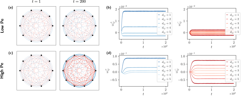
Learning to self-assemble and move.—Figure 2b shows that the system indeed learns asymmetric mobilities during training as long as Pe is large enough. These lead to the dynamic behavior during retrieval, where particles evolve according to Eq. (2) with the value of the interactions obtained at the end of the learning phase (Fig. 2c and Movie 2). We are now in the position of exploring what dynamic functionalities are enabled by this learning rule. We first choose the particles to self-assemble into a ring-like structure with the additional requirement of rotating on demand in either the clockwise or counter-clockwise direction (see Movie 2 and Fig. 2c). Note that despite the simplicity of the structure, we observe in Extended Data Fig. 3 that the learning rule leads to a complex graph of interactions that contribute to the stability of the ring.
Next, we train the particles (violet) to learn to self-assemble into a triangular formation and collectively chase a different target particle (orange) by imposing on them examples of the motion shown in Fig. 2d and Movie 2. During the retrieval period, we indeed see the particles self-assemble into a flying-wing shaped object (blue box) that cohesively maneuvers in space to chase (green box) and finally capture the moving target (red box).
As we illustrated with the LEGO toy in Movie 1, the examples in the training protocol (i.e. the motions imposed to the droplets or particles) should be time irreversible in order for the emergent time-delayed learning rule to produce asymmetric couplings. Here, it means that, for instance, particle 1 should systematically follow particle 2, as we demonstrate in Extended Data Fig. 2 and Movie 3.
Modified Hopfield spin model.—In order to to determine the basins of attraction and domain of existence of the fixed point and limit cycle solutions encoding the learned functionalities, we introduce a minimal model in which the time-delayed learning rule is put by hand rather than emergent. In this model, inspired by the Hopfield spin network [64, 65, 66, 67, 28, 29, 30, 31, 32, 37, 38, 68], the physical degrees of freedom are continuous spins following the equation
| (5) |
in which represent the effect of spin on spin . We consider the Hebbian-like learning rule with a time delay ,
| (6) |
in which controls the degree of asymmetry in time, while is a learning rate. Insights on the robustness of the learning phenomenon can already be obtained from considering the simplest non-trivial case of two spins.
In the training phase, a sinusoidal oscillation of the two spins is imposed, with or phase difference, corresponding to time-reversal symmetric or asymmetric training protocols respectively. We first confirm that the asymmetric coefficient are obtained only when the training examples are time-irreversible (Extended Data Fig. 2), very much like in the LEGO toy and particle based models. Furthermore, we can suppress completely by removing the delay (Methods). As a consequence, both fixed points and limit cycles can be obtained in the retrieval phase (Extended Data Fig. 2).
Learning on the fly.—So far, we have considered physical learning as a two-step process with separate training and retrieval phases. However, this strict distinction may be impractical in experiments. For instance, with the oil droplets of Fig. 1, the same physico-chemical processes are at play during training and retrieval, only with different Péclet numbers. Hence, the system may continue learning “on the fly” during retrieval, with potentially detrimental consequences if it ends up relaxing to an untrained state.
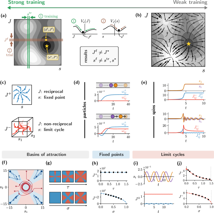
To assess the consequences of this intertwining, we formalize the training and retrieval process using a dynamical system perspective. The degrees of freedom in the system are split into degrees of freedom of interest (e.g. spins) and learning degrees of freedom (e.g. interactions between spins). The learning dynamics and the retrieval dynamics can be seen as two “slices” of a dynamical system handling both and (green and brown lines in Fig. 3a). In the limit of strong training, that we considered up to now, a trajectory is imposed by an external operator through the external field during the training period, leading to a learned that is frozen and used during the retrieval period. Another extreme case, that we call weak training, consists in reducing the training to setting an initial condition for , after which and simultaneously evolve towards the attractors of the dynamical system with (see Fig. 3), without the need of an external operator.
In Fig. 3, we have overlaid a unified “learning landscape” that schematically describes the relaxation of both training and physical degrees of freedom towards (dynamic or static) attractors 111Note that when depends on the past trajectory of the system, then in the figure represents the full past trajectory of the system. In practice, when does not only depend on the values of in the recent past, it approximated by the instantaneous values of , , , … up to a certain order.. In the case of non-potential dynamical systems, can be constructed as a Lyapunov function that captures the relaxation towards dynamic attractors such as limit cycles, but not the motion on the attractors [70]. As shown in Fig. 3b, we expect that the strong learning that we used up to now does not necessarily lead to minima of the learning landscape: the state obtained in the free evolution after learning may not exactly reproduce the training state (Fig. 3b).
This is indeed what we observe, in the particle system (see Methods, in which we also describe the effect of a finite training time) as well as in the minimal spin model with where exact solutions can be obtained (see Methods and Fig. 3h-j). Here, the training is reduced to the bare minimum of an initial condition for , while we set at the initial time . Figure 3f shows the results of our calculations of the basins of attraction of the fixed point (in blue) and limit cycles (in red): sufficiently asymmetric initial conditions spiral towards limit cycles, while more symmetric ones converge to fixed points. In the Methods, we show that an exact solution of the minimal model in Eq. 6 allows us to prove that the size of the basins of attraction is controlled by the degree of asymmetry and the time delay of the time-delayed learning rule (Fig. 3g). In addition, limit cycles disappear at critical values and (Fig. 3h-j). We find that, when the time delay is larger than the critical value , asymmetric interactions are suppressed before they can be learned. This suggests that there is a trade-off between large basins of attraction (at large ) and large non-reciprocity (at small but finite ).
To sum up, when the interactions are not frozen at the end of training, the system evolves towards its natural attractors, potentially leading to undesired configurations. However, the analysis behind Fig.3 reveals that one can also harness this feature as a shortcut to reduce the training time so that the evolution of the interactions and of the physical degrees of freedom reinforce each other.
Conclusions.—We have shown how to train and retrieve dynamic states through physical learning by combining time-delayed interactions, that emerge naturally from causal propagation, with a time-reversal asymmetric training protocol. This strategy can not only be applied in robotic matter by directly programming a computer, but also in physico-chemical active matter systems where it naturally emerges. Looking forward, programmable colloids based on DNA and other biomolecules [2, 58, 59, 60, 61, 62] would greatly enhance the potential complexity of learned behaviors by providing multiple interacting species and chemical feedback loops through enzymatic reactions. The principles illustrated here provide a step towards von Neumann’s dream of engineering synthetic living systems that adapt to the environment.
Materials and Methods
Proposal of experimental realization using chemotactic oil droplets
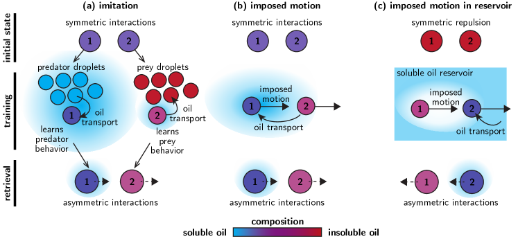
In this section, we discuss how a system of oil droplets that learn asymmetric interactions (such as that in Fig. 1e-f of the main text) can be realized experimentally. We suggest a recipe based on the chemotactic chasers from Ref. [18] but expect that learning rules with time delays could be implemented in other situations as long as there is an exergonic process coupled to the objects’ motion that can drive their dynamics.
The chasing droplets in Ref. [18] have asymmetric interactions that stem from asymmetric oil exchange. Two types of droplets, each consisting of an oil that is fully miscible with the oil in the other droplet, exchange oils through the aqueous continuous phase via micellar solubilization. One of the two oils is more soluble in the continuous phase than the other, so that the oil transport of droplet 1 to droplet 2 is faster than the transport of droplet 2 to droplet 1. The consequence is a net loss of soluble oil by droplet 1 and a net gain of soluble oil by droplet 2. This directional oil exchange leads to motion because the droplets tend to move away from areas with high solubilized oil concentrations; the solubilized oil increase the interfacial tension of the oil droplets driving a Marangoni flow. The droplets made of soluble oil thus moves toward the droplets made of the insoluble oil and, conversely, the droplet made of insoluble oil moves away from the droplet made of soluble oil. The net result is an asymmetric interaction where the soluble oil droplets act as predators and chase the insoluble oil droplets that act as prey.
The predator and prey droplets have an inherent memory effect through their composition; their oil exchange rate depends on their local chemical environment: droplets near predators lose less soluble oil, and droplets near prey lose more soluble oil. The droplets ‘remember’, through their composition, how many predator or prey droplets they have been near on average.
This memory effect could be used to have droplets of initially identical composition—and thus symmetric interactions—develop asymmetric interactions over time by evolving their oil exchange process in differing environments (Extended Data Fig. 1a). A mixed-composition droplet that spends time near mostly predator droplets loses less soluble oil (or may even gain soluble oil depending on its initial composition) so that its composition becomes more predator-like. Conversely, a mixed-composition droplet that spends time near mostly prey droplets loses more soluble oil and becomes more prey-like. When removed from their training chemical environment and placed together, the droplet that has evolved to a predator-like composition would likely chase the droplet that has evolved to a prey-like composition.
The same physical process of chemical-environment-dependent oil exchange could lead to droplets learning asymmetric interactions by the act of imposing the droplet motion in which the asymmetric interactions will result (Extended Data Fig. 1b). Imagine two droplets of equal mixed oil composition are forced to move in a pair with one droplet in front and the other at the back. When this motion if fast compared to diffusive transport (i.e. the Péclet number is much larger than one), the droplet in the back experiences a chemical environment with more soluble oil than the droplet in front. The back droplet can thus uptake oil from the front droplet but not the other way around, which causes the front droplet to have less soluble oil and become more prey-like, and the back droplet to have more soluble oil and become more predator-like.
Note that in the two cases described above, the training would be mechanistically similar to the retrieval. However, this is not necessarily the case: for instance, we expect that the same training protocol performed in a reservoir of soluble oil would cause the droplets to move in opposite directions during training and retrieval (Extended Data Fig. 1c).
Demonstration with LEGO toys
In Movie 1, we illustrate the ingredients required to learn dynamical states using a programmable toy. Two “Technic Medium Angular Motor” from a “LEGO Education SPIKE Prime” set are used, both as motors and angle sensors, to realize active XY-like spins. The LEGO toy is programmed to approximate the dynamics
| (7) |
in which label the XY spins with angles (see Ref. [40] for an exact solution of this dynamical system). This is realized by moving the positions of the robots by an increment every time step. In order to allow the user to move the spins by hand during the operation, the motors are also paused for a fixed time every time step.
In the training phase, the motors are disabled and time series of the angular positions imposed by the operator are recorded. The couplings are learned from these time series as
| (8) |
in which the memory kernel is taken as (and is set to zero for times going before the beginning of the recording). The parameters , , and are adjusted to be in a regime where learning is successful (see the main text for an analysis of the influence of training parameters).
Agent-based particle model
.0.1 Simulation details
As mentioned in the main text, for the particle based simulation we use overdamped dynamics of self-propelled particles following,
| (9) |
where is the position of the the particle, is the propulsion speed which acts along the direction . Here is a short range repulsive power law potential of the form
| (10) |
where and determines the energy scale and length scale of this steric interaction and is the cutoff distance. We have chosen , , and throughout our simulation. Also we have added the constant and the quadratic term in the potential to make both the potential and the corresponding force continuous at by choosing and . In the equation of motion mentioned above we used a small translational noise whose components are uniformly distributed between . The trained coefficients are used to determine the direction of self-propulsion mentioned before. The equation of motion for is
| (11) |
where represents the instantaneous target angle for the -th particle and it reflects the orientation of the vector . Note that this introduces a finite time relaxation mechanism in the orientational dynamics and in the limit , we get as mentioned in the main text. The timescale for the relaxation dynamics is controlled by and is a rotational noise which is uniformly distributed between . In the trial phase the system is initialised with randomised configuration of particles and zero pheromone concentration in the box. Particles then start releasing the pheromones (following Eq. 1 of the main text) and have constant self propulsive overdamped dynamics with speed which try to align towards a target angle , determined by the trained affinities .
.0.2 Order parameters
To identify the nature of the dynamic steady state observed during the trial in the particle based simulation, we construct the following order parameter for a pair ()
| (12) |
where is the unit vector associated with the propulsion vector of the th particle and is the unit vector along the line joining the pair (). This order parameter by construction will be zero for reciprocal attraction or repulsion as the center of mass velocity is zero when particle and either approach or run away from each other. However for a chase and run scenario, and the order parameter will be .
Field created by a particle moving at constant speed
In this section, we compute the steady-state field profile in the co-moving frame of reference of a particle moving at constant velocity . In this case, follows the equation
| (13) |
in which is the position of the particle (we set ). In the co-moving frame of reference, we define two coordinates and .
Modified Hopfield spin model
The model is defined by Eqs. (5) and (6) of the main text, for . It is convenient to introduce the symmetric and antisymmetric parts of the coupling (for , as the others are redundant).
.0.3 Role of delay time
In this section, we elucidate how the time delay in the learning rule enables the emergence of asymmetric interactions during training. Fig. 2 compares the outcome when the oscillatory training protocol of Fig. 2q-x is performed on the spin system with delay times (non-STDP) and (STDP). When the training protocol is time-reversal invariant (Fig. 2a), neither case results in non-reciprocity. However, when the training protocol breaks time-reversal invariance (Fig. 2b), it is only in the STDP case that results in after training. The non-STDP case has throughout the entire training period, even as oscillates around zero.
Indeed, when , the equation of motion for obtained from Eq. (6) becomes
| (19) |
so can only monotonically decay to zero. In contrast, may remain finite.
.0.4 Weak learning: exact solution for .
The dynamical system composed of spins , and their interactions and (or equivalently ) has fixed point and limit cycle steady states, as shown in Fig. 3b-d. Here, we exactly solve for these steady states, in particular to understand how they depend on the STDP parameters and . We have
| (20a) | ||||
| (20b) | ||||
| and | ||||
| (20c) | ||||
| and | ||||
| (20d) | ||||
Fixed points.
Fixed points are obtained by setting (note that this implies ). We obtain
| (21a) | ||||
| (21b) | ||||
| (21c) | ||||
where the signs of and are independent.
Limit cycles.
To find limit cycle solutions, we set (to match numerical observations) and assume that (we will later derive conditions for this to be true). In this case, we neglect in Eq. (20b) and obtain
| (22a) | |||
| (22b) | |||
where we assumed . We will solve for and derive conditions for this as as well.
Next, the solutions for can be placed into Eq. (20c) and (20d) to find . With , Eq. (20d) the relation between and s
| (23) |
while Eq. (20c) can be integrated to get
| (24) |
with
| (25) | ||||
| (26) |
We see that the initial assumption of is valid when is sufficiently close to 1, corresponding to the antisymmetric limit of STDP.
The steady state value of the amplitude is obtain using the above solutions for and as follows:
Averaging over a cycle of time (with denoting cycle average),
Note that can no longer be ignored since the contribution of vanishes. Then, the steady state solution yields
| (27) |
Similar to the condition on , the assumption is valid for close to 1.
Finally, we can use the solutions for (27) and (24) to eliminate these variables in Eq. (23). The resulting equation reads
| (28) |
and can be solved numerically for . Note that the solutions are identical upon interchanging spin indices 1 and 2.
Together, Eqs. (22), (24), (27), and (28) constitute the limit cycle solutions of the dynamical system as discussed in the text and shown in Fig. 3(d)(ii). We now derive the condition for existence of solutions that establishes the critical values and . The left side of Eq. (28) is maximized at , implying the condition
| (29) |
for limit cycle solutions to exist. Solutions vanish as or increase past the critical values.
.1 Sloppy trainer
In the main text we formulated the problem in such a way that during the training the trajectory of the learning particles were either perfectly micro-managed by the trainer or left completely free during the self learning. We now ask, what happens if the trainer is sloppy i.e. the scenario is between these two extremes.
We address this in two different ways: (a) by reducing the spatial control and (b) by decreasing temporal one. To understand the role of sloppiness of the trainer, we consider that the particles are confined in an annular domain (which acts as a quasi-linear track with harmonic confinement with stiffness ) during the training. In this set up, the particles are supposed to perform a periodic circular motion during the training. The presence of the trainer is implemented in the equation of motion of the learning particles via a tangential flow field (here is the unit vector along the azimuthal direction) along with a uniformly distributed translational noise,
| (30) |
For the first part, i.e. for lack of spatial control, we use a time independent flow where . One can see that this training protocol does not preserve the relative distance between the particles and therefore due to the fluctuations in the inter-particle distance the learned coefficients shows giant fluctuations compared to the case where the training is carried out by a strict trainer (see Fig. 4(a)). This fluctuations lead to set of learned that is insufficient to retrieve the assembly where the system was trained. The particles can still learn meaningful interactions during the learning process by ramping up the time scale associated with learning or (see Eq.3 of the main text). In the last panel of Fig. 4(a) one can see the coefficients reach similar values as compared to the case which is carried out by a strict trainer. This suggests when the trainer is sloppy a slow learner (with larger ) is a better learner.
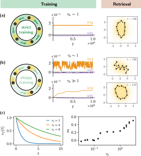
Next, to understand the role of temporal control, the flow field is slowly withdrawn (in an exponential manner) with a timescale (see Fig. 4(b)). In this case we combine both training and retrieval into a single process where the particles keeps on learning on the fly and interact via the instantaneous values learned interaction. Now the question we ask is, how large has to be so that the particles learn to systematically circle around in the annular chamber. Fig. 4(c) shows if particles don’t learn anything meaningful or (measured by a dynamic order parameter where is the unit vector along the azimuthal direction measured at position at the steady state) whereas with the performance during the trial is significant ().
.2 Movies
Supplementary movies are available in the following web link: https://home.uchicago.edu/~vitelli/videos.html.
References
- Hebb [2002] D. O. Hebb, The Organization of Behavior: A Neuropsychological Theory (L. Erlbaum Associates, Mahwah, N.J, 2002).
- Stern and Murugan [2023] M. Stern and A. Murugan, Learning Without Neurons in Physical Systems, Annual Review of Condensed Matter Physics 14, 417 (2023).
- Keim et al. [2019] N. C. Keim, J. D. Paulsen, Z. Zeravcic, S. Sastry, and S. R. Nagel, Memory formation in matter, Reviews of Modern Physics 91, 035002 (2019).
- Scheibner et al. [2022] C. Scheibner, M. Fruchart, and V. Vitelli, Soft metamaterials: Adaptation and intelligence (2022), arXiv:2205.01867 .
- Murugan et al. [2015] A. Murugan, Z. Zeravcic, M. P. Brenner, and S. Leibler, Multifarious assembly mixtures: Systems allowing retrieval of diverse stored structures, Proceedings of the National Academy of Sciences 112, 54 (2015).
- Falk et al. [2023a] M. J. Falk, J. Wu, A. Matthews, V. Sachdeva, N. Pashine, M. L. Gardel, S. R. Nagel, and A. Murugan, Learning to learn by using nonequilibrium training protocols for adaptable materials, Proceedings of the National Academy of Sciences 120, 10.1073/pnas.2219558120 (2023a).
- Pashine et al. [2019] N. Pashine, D. Hexner, A. J. Liu, and S. R. Nagel, Directed aging, memory, and nature’s greed, Science Advances 5, 10.1126/sciadv.aax4215 (2019).
- Stern et al. [2022] M. Stern, S. Dillavou, M. Z. Miskin, D. J. Durian, and A. J. Liu, Physical learning beyond the quasistatic limit, Physical Review Research 4, l022037 (2022).
- McMullen et al. [2022] A. McMullen, M. Muñoz Basagoiti, Z. Zeravcic, and J. Brujic, Self-assembly of emulsion droplets through programmable folding, Nature 610, 502–506 (2022).
- Glotzer [2004] S. C. Glotzer, Some assembly required, Science 306, 419–420 (2004).
- Lee et al. [2022] S. Lee, H. A. Calcaterra, S. Lee, W. Hadibrata, B. Lee, E. Oh, K. Aydin, S. C. Glotzer, and C. A. Mirkin, Shape memory in self-adapting colloidal crystals, Nature 610, 674–679 (2022).
- Djellouli et al. [2024] A. Djellouli, B. Van Raemdonck, Y. Wang, Y. Yang, A. Caillaud, D. Weitz, S. Rubinstein, B. Gorissen, and K. Bertoldi, Shell buckling for programmable metafluids, Nature 628, 545–550 (2024).
- Evans et al. [2024] C. G. Evans, J. O’Brien, E. Winfree, and A. Murugan, Pattern recognition in the nucleation kinetics of non-equilibrium self-assembly, Nature 625, 500–507 (2024).
- Wang et al. [2023] T. Wang, C. Pierce, V. Kojouharov, B. Chong, K. Diaz, H. Lu, and D. I. Goldman, Mechanical intelligence simplifies control in terrestrial limbless locomotion, Science Robotics 8, 10.1126/scirobotics.adi2243 (2023).
- Aguilar et al. [2016] J. Aguilar, T. Zhang, F. Qian, M. Kingsbury, B. McInroe, N. Mazouchova, C. Li, R. Maladen, C. Gong, M. Travers, R. L. Hatton, H. Choset, P. B. Umbanhowar, and D. I. Goldman, A review on locomotion robophysics: the study of movement at the intersection of robotics, soft matter and dynamical systems, Reports on Progress in Physics 79, 110001 (2016).
- King et al. [2023] E. M. King, C. X. Du, Q.-Z. Zhu, S. S. Schoenholz, and M. P. Brenner, Programmable patchy particles for materials design (2023), arXiv:2312.05360 .
- Niu et al. [2019] R. Niu, C. X. Du, E. Esposito, J. Ng, M. P. Brenner, P. L. McEuen, and I. Cohen, Magnetic handshake materials as a scale-invariant platform for programmed self-assembly, Proceedings of the National Academy of Sciences 116, 24402–24407 (2019).
- Meredith et al. [2020] C. H. Meredith, P. G. Moerman, J. Groenewold, Y.-J. Chiu, W. K. Kegel, A. van Blaaderen, and L. D. Zarzar, Predator–prey interactions between droplets driven by non-reciprocal oil exchange, Nature Chemistry 12, 1136–1142 (2020).
- Moran and Posner [2017] J. L. Moran and J. D. Posner, Phoretic self-propulsion, Annual Review of Fluid Mechanics 49, 511–540 (2017).
- Michelin [2023] S. Michelin, Self-propulsion of chemically active droplets, Annual Review of Fluid Mechanics 55, 77–101 (2023).
- Nguyen and Stebe [2002] V. X. Nguyen and K. J. Stebe, Patterning of small particles by a surfactant-enhanced marangoni-bénard instability, Physical Review Letters 88, 164501 (2002).
- Maass et al. [2016] C. C. Maass, C. Krüger, S. Herminghaus, and C. Bahr, Swimming droplets, Annual Review of Condensed Matter Physics 7, 171–193 (2016).
- Michelin et al. [2013] S. Michelin, E. Lauga, and D. Bartolo, Spontaneous autophoretic motion of isotropic particles, Physics of Fluids 25, 10.1063/1.4810749 (2013).
- Izri et al. [2014] Z. Izri, M. N. van der Linden, S. Michelin, and O. Dauchot, Self-propulsion of pure water droplets by spontaneous marangoni-stress-driven motion, Physical Review Letters 113, 248302 (2014).
- Schmitt and Stark [2013] M. Schmitt and H. Stark, Swimming active droplet: A theoretical analysis, EPL (Europhysics Letters) 101, 44008 (2013).
- Soto and Golestanian [2014] R. Soto and R. Golestanian, Self-assembly of catalytically active colloidal molecules: Tailoring activity through surface chemistry, Physical Review Letters 112, 068301 (2014).
- Moerman et al. [2017] P. G. Moerman, H. W. Moyses, E. B. van der Wee, D. G. Grier, A. van Blaaderen, W. K. Kegel, J. Groenewold, and J. Brujic, Solute-mediated interactions between active droplets, Physical Review E 96, 032607 (2017).
- Parisi [1986] G. Parisi, Journal of Physics A: Mathematical and General 19, L675–L680 (1986).
- Crisanti and Sompolinsky [1987] A. Crisanti and H. Sompolinsky, Dynamics of spin systems with randomly asymmetric bonds: Langevin dynamics and a spherical model, Physical Review A 36, 4922–4939 (1987).
- Sompolinsky and Kanter [1986] H. Sompolinsky and I. Kanter, Temporal association in asymmetric neural networks, Physical Review Letters 57, 2861–2864 (1986).
- Kanter and Sompolinsky [1987] I. Kanter and H. Sompolinsky, Mean-field theory of spin-glasses with finite coordination number, Physical Review Letters 58, 164–167 (1987).
- Kleinfeld [1986] D. Kleinfeld, Sequential state generation by model neural networks., Proceedings of the National Academy of Sciences 83, 9469–9473 (1986).
- Herron et al. [2023] L. Herron, P. Sartori, and B. Xue, Robust retrieval of dynamic sequences through interaction modulation, PRX Life 1, 023012 (2023).
- Dehaene et al. [1987] S. Dehaene, J. P. Changeux, and J. P. Nadal, Neural networks that learn temporal sequences by selection., Proceedings of the National Academy of Sciences 84, 2727–2731 (1987).
- Buhmann and Schulten [1987] J. Buhmann and K. Schulten, Noise-driven temporal association in neural networks, Europhysics Letters (EPL) 4, 1205–1209 (1987).
- Kleinfeld and Sompolinsky [1988] D. Kleinfeld and H. Sompolinsky, Associative neural network model for the generation of temporal patterns. theory and application to central pattern generators, Biophysical Journal 54, 1039–1051 (1988).
- Hertz et al. [1987] J. A. Hertz, G. Grinstein, and S. A. Solla, Irreversible spin glasses and neural networks, in Lecture Notes in Physics (Springer Berlin Heidelberg, 1987) p. 538–546.
- Hertz et al. [1986] J. A. Hertz, G. Grinstein, and S. A. Solla, Memory networks with asymmetric bonds, in AIP Conference Proceedings (AIP, 1986).
- Ivlev et al. [2015] A. V. Ivlev, J. Bartnick, M. Heinen, C.-R. Du, V. Nosenko, and H. Löwen, Statistical mechanics where newton’s third law is broken, Physical Review X 5, 011035 (2015).
- Fruchart et al. [2021] M. Fruchart, R. Hanai, P. B. Littlewood, and V. Vitelli, Non-reciprocal phase transitions, Nature 592, 363 (2021).
- Saha et al. [2020] S. Saha, J. Agudo-Canalejo, and R. Golestanian, Scalar active mixtures: The nonreciprocal cahn-hilliard model, Physical Review X 10, 041009 (2020).
- You et al. [2020] Z. You, A. Baskaran, and M. C. Marchetti, Nonreciprocity as a generic route to traveling states, Proceedings of the National Academy of Sciences 117, 19767 (2020).
- Yifat et al. [2018] Y. Yifat, D. Coursault, C. W. Peterson, J. Parker, Y. Bao, S. K. Gray, S. A. Rice, and N. F. Scherer, Reactive optical matter: light-induced motility in electrodynamically asymmetric nanoscale scatterers, Light: Science and Applications 7, 10.1038/s41377-018-0105-y (2018).
- Drescher et al. [2009] K. Drescher, K. C. Leptos, I. Tuval, T. Ishikawa, T. J. Pedley, and R. E. Goldstein, Dancing volvox: Hydrodynamic bound states of swimming algae, Physical Review Letters 102, 168101 (2009).
- Osat and Golestanian [2022] S. Osat and R. Golestanian, Non-reciprocal multifarious self-organization, Nature Nanotechnology 18, 79–85 (2022).
- Baek et al. [2018] Y. Baek, A. P. Solon, X. Xu, N. Nikola, and Y. Kafri, Generic long-range interactions between passive bodies in an active fluid, Physical Review Letters 120, 058002 (2018).
- Banerjee et al. [2022] J. P. Banerjee, R. Mandal, D. S. Banerjee, S. Thutupalli, and M. Rao, Unjamming and emergent nonreciprocity in active ploughing through a compressible viscoelastic fluid, Nature Communications 13, 4533 (2022).
- Dinelli et al. [2023] A. Dinelli, J. O’Byrne, A. Curatolo, Y. Zhao, P. Sollich, and J. Tailleur, Non-reciprocity across scales in active mixtures, Nature Communications 14, 10.1038/s41467-023-42713-5 (2023).
- Mandal et al. [2022] R. Mandal, S. S. Jaramillo, and P. Sollich, Robustness of travelling states in generic non-reciprocal mixtures (2022), arXiv:2212.05618 [cond-mat.stat-mech] .
- Avni et al. [2023] Y. Avni, M. Fruchart, D. Martin, D. Seara, and V. Vitelli, The non-reciprocal ising model (2023), arXiv:2311.05471 .
- Abbott and Nelson [2000] L. F. Abbott and S. B. Nelson, Synaptic plasticity: taming the beast, Nature Neuroscience 3, 1178–1183 (2000).
- Dan and Poo [2004] Y. Dan and M.-m. Poo, Spike timing-dependent plasticity of neural circuits, Neuron 44, 23–30 (2004).
- Caporale and Dan [2008] N. Caporale and Y. Dan, Spike Timing–Dependent Plasticity: A Hebbian Learning Rule, Annual Review of Neuroscience 31, 25 (2008).
- Shouval [2010] H. Shouval, Spike timing dependent plasticity: A consequence of more fundamental learning rules, Frontiers in Computational Neuroscience 10.3389/fncom.2010.00019 (2010).
- Song et al. [2000] S. Song, K. D. Miller, and L. F. Abbott, Competitive Hebbian learning through spike-timing-dependent synaptic plasticity, Nature Neuroscience 3, 919 (2000).
- Fiete et al. [2010] I. R. Fiete, W. Senn, C. Z. Wang, and R. H. Hahnloser, Spike-time-dependent plasticity and heterosynaptic competition organize networks to produce long scale-free sequences of neural activity, Neuron 65, 563–576 (2010).
- Jambon-Puillet et al. [2024] E. Jambon-Puillet, A. Testa, C. Lorenz, R. W. Style, A. A. Rebane, and E. R. Dufresne, Phase-separated droplets swim to their dissolution, Nature Communications 15, 10.1038/s41467-024-47889-y (2024).
- Fredriksson et al. [2002] S. Fredriksson, M. Gullberg, J. Jarvius, C. Olsson, K. Pietras, S. M. Gústafsdóttir, A. Östman, and U. Landegren, Protein detection using proximity-dependent dna ligation assays, Nature Biotechnology 20, 473–477 (2002).
- Schaus et al. [2017] T. E. Schaus, S. Woo, F. Xuan, X. Chen, and P. Yin, A dna nanoscope via auto-cycling proximity recording, Nature Communications 8, 10.1038/s41467-017-00542-3 (2017).
- Moerman et al. [2023] P. G. Moerman, H. Fang, T. E. Videbæk, W. B. Rogers, and R. Schulman, A simple method to alter the binding specificity of dna-coated colloids that crystallize, Soft Matter 19, 8779–8789 (2023).
- Weinstein et al. [2019] J. A. Weinstein, A. Regev, and F. Zhang, Dna microscopy: Optics-free spatio-genetic imaging by a stand-alone chemical reaction, Cell 178, 229 (2019).
- Owen et al. [2023] J. A. Owen, D. Osmanović, and L. Mirny, Design principles of 3d epigenetic memory systems, Science 382, 10.1126/science.adg3053 (2023).
- Falk et al. [2023b] M. Falk, A. Strupp, B. Scellier, and A. Murugan, Contrastive learning through non-equilibrium memory (2023b), arXiv:2312.17723 .
- Hopfield [1982] J. J. Hopfield, Neural networks and physical systems with emergent collective computational abilities., Proceedings of the National Academy of Sciences 79, 2554–2558 (1982).
- Ramsauer et al. [2020] H. Ramsauer, B. Schäfl, J. Lehner, P. Seidl, M. Widrich, T. Adler, L. Gruber, M. Holzleitner, M. Pavlović, G. K. Sandve, V. Greiff, D. Kreil, M. Kopp, G. Klambauer, J. Brandstetter, and S. Hochreiter, Hopfield networks is all you need (2020), arXiv:2008.02217 .
- Hopfield [1984] J. J. Hopfield, Neurons with graded response have collective computational properties like those of two-state neurons., Proceedings of the National Academy of Sciences 81, 3088–3092 (1984).
- Koiran [1994] P. Koiran, Dynamics of discrete time, continuous state hopfield networks, Neural Computation 6, 459–468 (1994).
- Clark and Abbott [2024] D. G. Clark and L. Abbott, Theory of coupled neuronal-synaptic dynamics, Physical Review X 14, 021001 (2024).
- Note [1] Note that when depends on the past trajectory of the system, then in the figure represents the full past trajectory of the system. In practice, when does not only depend on the values of in the recent past, it approximated by the instantaneous values of , , , … up to a certain order.
- Fang et al. [2019] X. Fang, K. Kruse, T. Lu, and J. Wang, Nonequilibrium physics in biology, Reviews of Modern Physics 91, 045004 (2019).
- [71] DLMF, NIST Digital Library of Mathematical Functions, https://dlmf.nist.gov/, Release 1.1.10 of 2023-06-15 (2023), f. W. J. Olver, A. B. Olde Daalhuis, D. W. Lozier, B. I. Schneider, R. F. Boisvert, C. W. Clark, B. R. Miller, B. V. Saunders, H. S. Cohl, and M. A. McClain, eds.