Capacity bounds on integral flows
and the Kostant partition function
Abstract.
The type Kostant partition function is an important combinatorial object with various applications: it counts integer flows on the complete directed graph, computes Hilbert series of spaces of diagonal harmonics, and can be used to compute weight and tensor product multiplicities of representations. In this paper we study asymptotics of the Kostant partition function, improving on various previously known lower bounds and settling conjectures of O’Neill and Yip. Our methods build upon recent results and techniques of Brändén-Leake-Pak, who used Lorentzian polynomials and Gurvits’ capacity method to bound the number of lattice points of transportation and flow polytopes. Finally, we also give new two-sided bounds using the Lidskii formulas from subdivisions of flow polytopes.
1. Introduction
Integer flows on networks are very important objects in optimization, combinatorics, and representation theory. In the latter context, the number of integer flows on a directed complete graph is also known in Lie theory as the Kostant partition function. Many important quantities in representation theory like weight multiplicities (like Kostka numbers) and tensor product multiplicities (like the Littlewood–Richardson coefficients) can be expressed in terms of this function [Hum08]. In this paper, we give new lower bounds on the Kostant vector partition function that improve on previously known bounds. To do this, we utilize recent lower bounds on the number of contingency tables given in [BLP23]. Contingency tables are the lattice points of transportation polytopes, and since flow polytopes can be seen as faces of transportation polytopes, we are able to adapt the results of [BLP23] to our context. The bounds of [BLP23] come via lower bounds on the coefficients of certain (denormalized) Lorentzian polynomials [BH20, AOGV21, Gur09a] and their associated generating series, in terms of their capacity [Gur06a]. Our main contribution is then new explicit estimates of the capacity of these generating series via an associated flow entropy quantity, which lead to our new lower bounds.
Let where and let be a directed acyclic connected graph with vertices . We denote by the flow polytope of with netflow . When is the complete graph , we denote by the flow polytope by . We are interested in the number of lattice points of the flow polytope , i.e. the number of integer flows of the complete graph with netflow . This is called the Kostant vector partition function since it has an interpretation in the representation theory of Lie algebras: it is the number of ways of writing as an -combination of the vectors for , the type positive roots.
The function is a piecewise-polynomial function on the parameters 111Note that this does not imply polynomial bounds on , since the total degree of the polynomials can depend on the length of the vector (see Section 6). [Stu95] with a complex chamber structure [GMP21, BBCV06]. Moreover, computing the number of lattice points of in general is a computationally hard problem [BSDLV04], and there are special cases that are important and give surprising answers. We list a few of these, see Section 2.3 for more details.
-
(i)
, however no general formula is known for which is the Ehrhart polynomial of the flow polytope . Chan–Robbins–Yuen [CRY00] showed that for , the sequence satisfies a linear recurrence of order , the number of integer partitions of . Moreover, the following bounds are known for
(1.1) The lower bound follows from elementary methods, and improving this bound with more interesting techniques has proven elusive. The upper bound is more subtle and it follows from containment of in another polytope related to alternating sign matrices [MMS19].
- (ii)
-
(iii)
, this value counts the number of Tesler matrices [Hag11, AGH+12] which are of interest in the study of the space of diagonal harmonics which has dimension (see [Hag08]), the number of rooted forests on vertices . Indeed, there is a formula of Haglund [Hag11] for the Hilbert series of this space as an alternating sum over the integer flows counted in . No simple formula is known for but from the connection to and computational evidence [Inc, A008608] it is expected that eventually . This is a special case of [O’N18, Conj. 6.5]. In an effort to show this lower bound, O’Neill [O’N18] found the following bounds for ,
(1.2) Note that . In 2016 Pak (private communication) asked whether is and in 2019 Yip conjectured (private communication) that for all , is at least as big as the number of forests on vertices [Inc, A001858], which is also the number of lattice points of the permutahedron .
-
(iv)
where is the sum of all positive roots in type [Inc, A214808]. The quantity gives the dimension of the zero weight space of a certain Verma module [Hum08] and the problem of giving bounds for this quantity was raised in [hs]. O’Neill obtained in [O’N15] the following bound for when ,
(1.3) He also gave a bound for (see Proposition 2.23).
These cases suggest studying the asymptotic behavior of the Kostant partition function. In this paper we obtain the following improvements for the all cases mentioned above.
Theorem 1.1.
Fix an integer and let . Then for we have
The big-O notation is with respect to (with parameter fixed), and the implied constant is independent of and .
This improves over the bound from the lower bound in (1.1) by an extra factor of .
For the Tesler case , we have the following lower bound222After the paper was finished, Anne Dranowski kindly informed us that in a forthcoming paper with Ivan Balashov, Constantine Bulavenko, and Yaroslav Molybog they obtain a lower bound (June 13, 2024, personal communication)..
Theorem 1.2.
Let . Then for we have
Furthermore, for .
This bound beats (asymptotically) all previously known bounds (1.2) and proves Yip’s and O’Neill’s conjectures mentioned above, for large enough , since . This bound is the first improvement beyond towards answering Pak’s question.
As a comparison, in the case where has a closed formula and thus [MS21, Lemma 7.4], our methods give the lower bound . For all polynomial growth cases we also obtain a general bound. (We also obtain better bounds for more specific cases; see Section 5.)
Theorem 1.3.
Fix and and suppose for all . Then
The symbol means the expressions given above essentially give the leading term of the actual lower bounds we obtain. See Theorem 5.1 for the formal statement of this result.
The phase transitions in the above lower bounds are possibly interesting, but we cannot tell whether or not they are artifacts of our proof strategy. See Section 7.3 for further discussion.
The final case we discuss is that of . This case does not fit with the previous cases in the sense that some entries of are negative, but we are still able to apply our methods to achieve the following lower bound.
Theorem 1.4.
Fix an integer and let . Then for we have
The implied constant is independent of .
This bound improves over the results of O’Neill for all integers (see above and Proposition 2.23), including the important case of where we improve the leading-term constant for from to .
Finally, we prove bounds in various other specific cases using the same methods, and these are collected in Section 5.
Methodology
To state our main result we need the following notation. Given some flow and letting we define the flow entropy of via
| (1.4) |
Note that is a concave function on . With this, we can now state the main technical result we use to prove our bounds.
Theorem 1.5 (flow version of [Bar10, Lemma 2.2], [Bar12, Lemma 5], [BLP23, Thm. 3.2]).
Let be an integer vector such that is non-empty, and let for all . Letting denote the number of integer points of , we have
Results similar to Theorem 1.5 have appeared in various contexts before, as suggested by the cited references. That said, we give a new and streamlined proof technique for this fact in Section 3.
Using Theorem 1.5, we can obtain explicit lower bounds on for a given flow vector by computing
| (1.5) |
for a well-chosen . The which optimizes has no closed-form formula in general, and thus some heuristic must be used to choose which yields good bounds. The potential problem with this approach is that asymptotic formulas for may have phase transitions (see [LP22, DLP20] for examples of this in the context of contingency tables); that is, it is possible that similar values of can lead to different asymptotics. This means that a too-simple heuristic leading to a general formula for a lower bound on is unlikely to give a high quality bound.
With this in mind, we devise a heuristic for choosing which is complicated enough to hopefully allow for good bounds, but simple enough to be applicable to a wide range of values of . Specifically, we choose to be the average of the vertices of . On the one hand, counting and computing the average of the vertices of a given flow polytope can be non-trivial in general. On the other, we demonstrate the quality of this choice by proving lower bounds in various cases which are asymptotically better than all previously known bounds.
Finally, once we have our choice of , we extract explicit asymptotics from the flow entropy expression (1.5) evaluated at . This last step, while elementary, requires some not-so-trivial analysis of the entropy function via the Euler-Maclaurin formula.
|
A result for intuition
Theorem 1.5 above suggests that a well-chosen can produce good lower bounds on , and the improved bounds we are able to prove in this paper perhaps demonstrate this for some particular cases. We now state a result which demonstrates this more generally, and offers some more formal evidence why we expect the ideas of this paper to yield good bounds on the number of flows (see Section 5.9 for the proof).
Theorem 1.6.
Let be an infinite sequence of positive integers which has at most polynomial growth, and let and for all . Then the maximum flow entropy asymptotically approximates . That is, as we have
That is, there is some choice of flows (dependent on ) which produces the correct asymptotics in the . This perhaps makes the problem simpler for the positive polynomial growth case of Theorem 1.6: instead of counting lattice points of polytopes, we just need to find choices of (not necessarily integer) flows with high entropy. We also remark that in Theorem 1.6 can be replaced by the more standard geometric entropy: .
Bounds for other regimes
Finally, in the results above we mainly consider the individual entries of the flow vector to be constant with respect to . For example, in the case of in Theorem 1.1, we fix and bound the asymptotics with respect to . However, there are other regimes where bounds are desirable; for example, may itself be a function of .
To handle cases like this, we use a different technique. Specifically, we use a positive formula for called the Lidskii formula [BV08, MM19] coming from the theory of flow polytopes and related to mixed volumes to give bounds for for much larger than .
Theorem 1.7.
For we have that
These concrete bounds are reasonable compared to the leading coefficient in of , the volume of the polytope [Zei99].
The techniques used for these bounds do not fit directly into the overarching methodology discussed above. That said, we include them anyway for completeness, and due to the connection between the Lidskii formula and mixed volumes. Mixed volumes are the coefficients of volume polynomials, which are Lorentzian (see, e.g., [BH20]), and thus there may be some further connection between this formula and the entropy-based methodology discussed above. We leave this to future work.
Structure of the paper
The paper is organized as follows. Section 2 has background on flow polytopes, bounds, capacity method on contingency tables, and asymptotics of entropy related functions. Section 3 gives our proof of Theorem 1.5. Section 4 has details on the averages of vertices of flow polytopes. Section 5 computes the concrete asymptotic lower bounds for all the cases we consider. Section 6 gives bounds on the Kostant partition function using the Lidskii formula from the theory of flow polytopes. Section 7 has final remarks. Details of the asymptotic analysis are in the Appendix A.
2. Background and combinatorial/geometric bounds
2.1. Transportation and flow polytopes
A polytope is a convex hull of finitely many points or alternatively a bounded intersection of finitely many half spaces. The polytopes we consider are integral, i.e. its vertices have integer coordinates. Two polytopes and are integrally equivalent if there is an affine transformation such that restricted to and gives a bijection and to . Next, we define flow polytopes and transportation polytopes.
Definition 2.1 (Transportation polytopes).
Let and be vectors in , the transportation polytope is the set of all matrices with nonnegative real entries with row sums and column sums and . The lattice points of are called contingency tables and we denote the number of such tables by .
The generating function of has the following closed form.
| (2.1) |
Definition 2.2 (flows and flow polytope).
Given a a directed acyclic graph with vertices and edges, and a vector , an -flow on is a tuple in of values assigned to each edge such that the netflow on vertex is :
The flow polytope is the set of -flows on .
When is the complete graph , for brevity we denote by the flow polytope . We denote by the number of lattice points of , which counts the number of integer flows on with netflow . This is called Kostant’s vector partition function since it also counts the number of ways of writing as a combination of the positive type- roots corresponding to each edge where is a standard basis vector.
The generating function of for has the following closed form.
| (2.2) |
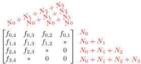
Flow polytopes can be viewed as faces of transportation polytopes as follows (see [MMR17, §1.3]). Given a flow vector , define and where as above. Define a linear injection via
| (2.3) |
where the subdiagonal entries are chosen so that the row sums and column sums are equal to the entries of and . (Note that these entries are given precisely by for ). The image of is the set matrices in which have in all entries of the bottom-right corner of the matrix as specified in the definition of . The set is a face of (see [MMR17, Prop. 1.5]).
By abuse of notation, we will refer to a flow in and its image in interchangeably.
Proposition 2.3 ([MMR17, Prop. 1.5]).
Given , and , , and be defined as above, then is an integral equivalence between and a face of .
2.2. Special examples of flow polytopes
The following are two examples of flow polytopes that will be of interest and we give their vertex description.
2.2.1. CRY polytope
For , the polytope is called the Chan-Robbins-Yuen polytope [CRY00]. This polytope has dimension and vertices [CRY00]. The vertices can be described as follows: they correspond to unit flows along paths on from the source to the sink . These paths are completely determined by their support on internal vertices in . We translate the description of these vertices in the transportation polytope.
Proposition 2.4.
For , the vertices of are determined by binary strings in the sub-diagonal: . In particular there are vertices.
Given a binary string , the corresponding vertex given by
| (2.4) |
where .
Since is a polytope, its lattice points are its vertices and so .
2.2.2. Generalized Tesler polytope
For ( where ) , the polytope is called the (generalized) Tesler polytope [MMR17]. This polytope has dimension , is simple, and has vertices. The vertices can be characterized as follows.
Theorem 2.5 ([MMR17, Thm. 2.5 & Cor. 2.6]).
For where , the vertices of are characterized by flows whose associated matrix has exactly one nonzero upper triangular entry in each row. In particular there are vertices.
Given a choice of an upper triangular entry in each row, the corresponding vertex is defined by
| (2.5) |
and the sub-diagonal term is for .
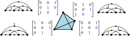
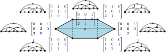
Example 2.6.
The CRY polytope is -dimensional with vertices/lattice points represented by the following matrices:
The Tesler polytope is -dimensional with the following seven lattice points of which the first six are its vertices:
See Figure 2.
2.3. Previous bounds on lattice points of flow polytopes
In this section we collect previous results and questions about bounds on . See Table 1.
Proposition 2.7 (e.g. [O’N18, §2.1]).
Let , then
| (2.6) |
where the sum is over integer flows in .
Given weak compositions and , we say that dominates if for every and denote it by .
Proposition 2.8.
Let and where and are in such that , then .
Proof.
Let for , and ( and , respectively) where (for ). Given an integer flow of viewed as a lattice point in , let be defined as
Then is an integer flow in , i.e. is a lattice point in . This map is injective and therefore , as desired. ∎
In particular, the previous result implies a similar inequality when is term-wise larger than .
Corollary 2.9.
Let and where and are in such that then .
2.3.1. The cases with closed formulas
The following cases of have closed formulas coming from a certain constant term identity due to Zeilberger [Zei99], that is a variation of the Morris constant term identity related to the Selberg integral. For self contained proofs of these product formulas see [BSV04, MS21]. Let denote the th Catalan number and let
which counts the number of plane partitions of shape with entries at most in [Pro90].
Remark 2.11.
By a result of Postnikov–Stanley (unpublished) and Baldoni–Vergne [BV08], we have the following relation between the normalized volume of equals a value of ,
| (2.8) |
where the second equality follows by setting in (2.7). Moreover, the leading term in of (2.7) gives the normalized volume of [MMR17, Theorem 1.8], [ZLF17, Lemma 2.1].
where is the number of Standard Young tableaux of shape .
The next two results collect asymptotics and bounds for the special cases and the pieces of the product on the RHS of (2.7)
Proposition 2.12 ([MS21, Lemma 7.4]).
Proposition 2.13 ([MS21, Proposition 7.5]).
Proposition 2.14 ([MPP19, Proposition 3.1]).
For all integers and we have that
where .
2.3.2. The CRY case
Proposition 2.15 (upper bound from [MMS19]).
For we have that
Proof.
Theorem 2.16 (Chan–Robbins–Yuen [CRY00, Thm. 1]).
Fix an integer and let , then satisfies a linear recurrence of order , the number of integer partitions of . In particular for some constant .
2.3.3. The Tesler case
Proposition 2.17.
For we have that
Proof.
A more careful analysis of Proposition 2.7 was performed by O’Neill to improve the bounds for the case of .
Proposition 2.18 (O’Neill [O’N18]).
Let be the classical permutahedron. In 2019, Yip (private communication) asked whether the Tesler polytope projects to the permutahedron and conjectured the following weaker statement. Recall that is the number of forests with vertices [Inc, A001858]. This is also the number of lattice points of .
Conjecture 2.19 (Yip).
For , we have that .
Next, we give some other bounds for the number of lattice points of dilations of the Tesler polytope.
Proposition 2.20.
For then
| (2.9) |
Proof.
By Corollary 2.9 we have that
The upper bound follows by the product formula in (2.7) for the LHS above.
∎
Proposition 2.21.
For we have that
Proof.
Corollary 2.22.
Proof.
| no closed formula | |
| no closed formula | |
| no closed formula |
2.3.4. The case of
We next consider the case where is the sum of all the positive roots of the type root system, given by for . The quantity gives the dimension of the zero weight space of a certain Verma module [Hum08]. More concretely, we have
A post in [hs] raised the question of studying bounds for . In an unpublished report [O’N15], O’Neill using the techniques in [O’N18, §5] obtained the following bounds for and .
Proposition 2.23 ([O’N15]).
For a nonnegative odd integer and we have that
By taking the logs of the results above we immediately obtain the following results.
Corollary 2.24.
Fix an integer and let . We have that
and
2.4. Polynomial capacity and log-concave polynomials
Polynomial capacity, originally defined by Gurvits [Gur06a], is typically defined as follows. Note that here we extend the definition to multivariate power series.
Definition 2.25 (Polynomial and power series capacity).
Given a polynomial or power series with non-negative coefficients and any , we define
This equivalently defined as
where is the usual dot product.
The typical use of capacity is to approximate or bound the coefficients of certain polynomials or power series. For example, the following bound follows immediately from the definition.
Lemma 2.26.
Given a polynomial or power series with non-negative coefficients and any , we have
where denotes the coefficient of in .
Lower bounds in terms of the capacity, on the other hand, are harder to prove. In fact, one should not expect such lower bounds in general; e.g., and for . Thus lower bounds are typically only proven for certain classes of polynomials and power series. The most common classes are real stable polynomials, Lorentzian polynomials (also known as completely log-concave and strongly log-concave [BH20, AOGV21, Gur09a]), and most recently denormalized Lorentzian polynomials. Such bounds have been applied to various quantities, such as: the permanent, the mixed discriminant, and the mixed volume [Gur06a, Gur06b, Gur09b]; quantities related to matroids, like the number of bases of a matroid and the intersection of two matroids [SV17, AOG17, AOGV21, ALOGV24]; the number of matchings of a bipartite graph [GL21b]; and the number of contingency tables [Bar09, Gur15, BLP23]. We do not explicitly use results of definitions regarding these polynomial classes, but instead refer the interested reader to the above references.
2.5. Bounds on contingency tables
Given vectors and , recall that a contingency table is an matrix with non-negative integer entries, for which the row sums of and the column sums of are given by the entries of and respectively. (Recall also that we index the rows and columns starting with .) As discussed above, the set of all contingency tables has a nice generating function with coefficients indexed by and , given by
Lower bounds on in terms of the capacity of were obtained in [BLP23], which improved upon previous bounds of [Bar09, Gur15]. The bound for general contingency tables is given as follows.
Theorem 2.27 ([BLP23], Thm. 2.1).
Given and , we have
Note that starting from respectively is not a typo, and in fact we can replace the products above by a product over any subset of all but one of the factors.
Bounds are also achieved in [BLP23] for contingency tables with restricted entries, where then entries of a given matrix are bounded above entry-wise by a given matrix . We care in this paper specifically about the case when for and otherwise, for which we have that the number of contingency tables counts the number of integer flows as in (2.3). In this case, we define
and the bound is given as follows. Note that the authors of [BLP23] do not write their theorem in terms of flows explicitly, and so we translate their theorem here (in light of (2.3)) for the convenience of the reader.
Theorem 2.28 ([BLP23], Thm. 2.1).
Given , define for and let and . Then we have
In this paper, we will determine lower bounds for and combine this with the bound given by Theorem 2.28. AThis will lead to our new bounds on flows.
2.6. Convex analysis
Given a function , we define its domain via
We say is convex if is convex and is convex on . The convex conjugate (or Fenchel conjugate or Legendre transform) of is also a convex function, defined as follows.
Definition 2.29.
Given a convex function , its convex conjugate is a convex function defined via
We denote the domain of by .
In order to give lower bounds on the capacity of a given polynomial or generating series, we use an idea already present in the work of Barvinok (e.g. Lemma 5 of [Bar12]) and in Proposition 6.2 of [BLP23]: we convert the infimum in the definition of capacity (Definition 2.25) into a supremum. We can then lower bound the supremum by simply evaluating the objective function at any particular chosen value of the domain. A proof sketch for a general version of this is given in [BLP23], and we give a different and simpler proof in this paper based on the following classical result of convex analysis relating convex conjugates via the infimal convolution.
Theorem 2.30 ([Roc70], Thm. 16.4).
Let be a convex function given as the sum of convex functions with respective domains . If is non-empty then
where for each the infimum is attained. Note that the domain of optimization is over all choices of vectors such that .
3. A Dual Formulation for Capacity
As above, let denote the number of integer flows on with netflow given by . Counting such integer flows is equivalent to counting the integer matrices of the form given by (2.3), where the row and columns sums are given by and where . Thus by Theorem 2.28, we have
where
with .
In this section, we will utilize Theorem 2.30 to convert the infimum of the above capacity expression into a supremum. Specifically, we will prove the following.
Proposition 3.1.
Proposition 3.1 then leads immediately to the following result, which we will utilize in the later sections.
Theorem 3.2.
Let be any (not necessarily integer) point of , let , and let where is defined as in (2.3). We have that
There are also versions of the above results for the volumes of flow polytopes. Since these are outside the context of the results of this paper, we leave further discussion of these results to the final remarks (see Section 7.6).
3.1. Proof of Proposition 3.1
The second equality follows from the definition of flow entropy , and so we just need to prove the first equality. Consider the following function:
Here, as above, the variables are indexed from to . Since is a convex function on its domain, we have that is convex on its domain . Since is defined as a sum of convex functions, we can apply Theorem 2.30 to obtain
for any of the form described at the start of Section 3. Note that the sum under the is over all choices of vectors and (for and ) such that .
Here we have that
and the function is convex with domain given by
We then have
and by a straightforward argument this implies
Thus for any , standard calculus arguments give
Combining this with the above expressions then gives
Negating and exponentiating both sides then gives the desired result.
4. Computing the Average of Vertices of some flow polytopes
In this section we compute the uniform average of the vertices of the flow polytopes for with positive netflow and . We assume a uniform distribution on the vertices of the polytope. In abuse of notation we refer to all the entries on or above the antidiagonal, upper triangular entries (see Proposition 2.3).
Proposition 4.1.
For where the uniform average of the vertices of is the flow where , for . That is, it is represented by the matrix
| (4.1) |
where .
Proof.
Proposition 4.2.
For where the uniform average of vertices of is represented by the matrix where
| (4.2) |
Proof.
Let be desired uniform average for , and let be a uniformly random vertex. By Theorem 2.4, are i.i.d. uniform Bernoulli random variables for all , and . Using this and the description of the vertices of in (2.4), if then
Further, if exactly one of is equal to 0 then
And finally, if then
For the case for we have that , and so the uniform average of the vertices also dilates by . ∎
For the case that (where , see Section 2.3.4) with for all , we were unable to exactly compute the average of the vertices. However, a few experiments show that the average may be close to the following natural point in the flow polytope:
| (4.3) |
where the subdiagonal entries are given by for .
Remark 4.3.
As stated above, we were not able to compute the average of the vertices of where . The polytope for the cases have and vertices and averages:
It would be interesting to find the number of vertices and average for this case.
5. Flow Counting Lower Bounds
In this section we prove our main lower bounds on flows. Specifically we apply Theorem 3.2 to various flow vectors , using specific choices of flows given by the average of the vertices of the associated flow polytopes (as computed in Section 4). This technique yields lower bounds for the number of flows , often given in a relatively complicated product form. We then obtain more explicit lower bounds for the asymptotics of by combining the Euler-Maclaurin formula (see Lemma A.2) with a number of elementary bounds on entropy-like functions (see Lemma A.1 and the rest of Appendix A).
We now state the bounds obtained in the section in the following results, and the remainder of this section is devoted to proving these bounds. Throughout, as above, we let denote the netflow vector, and we denote . Any big-O notation used is always with respect to , with other parameters fixed. Also, we will sometimes put parameters in the subscripts of the big-O notation to denote that that implied constant may depend on those parameters.
Theorem 5.1 (Polynomial growth).
For for all , with given and ,
Note that the implied constant of the big-O notation may depend on and . Also note that the cases limit to the same bounds at .
Theorem 5.2 (Tesler case).
For ,
Further, for .
Theorem 5.3 (Other specific examples).
We have the following.
-
(1)
For ,
-
(2)
For for all , with given ,
-
(3)
For for all , with given ,
Note that the implied constant may depend on .
-
(4)
For for all ,
-
(5)
For , with given ,
The implied constant is independent of .
-
(6)
For , with given ,
The implied constant is independent of .
Remark 5.4.
5.1. Positive flows in general
Here we state some general lower bounds in the cases where every entry of the netflow vector is positive. Note though that these bounds hold even in the case where the netflow vector is only non-negative.
Theorem 5.5.
Fix (i.e., the entries are not necessarily non-negative). Denoting and , we have
-
(1)
If for all ,
-
(2)
If and for all ,
5.2. Polynomial growth
5.2.1. The case of .
5.2.2. The case of .
First,
is a lower bound on the possible values of which we will use throughout the case. Defining
we have
since is increasing in . Further note that since , we have
Theorem 5.5 (2) then implies
We now split into two subcases: and .
For , we have
and
We first use
which implies the following, where for :
Using and Corollary A.4 gives
Next, a straightforward computation gives
since this expression is increasing in because is increasing for . Using Lemma A.3 we have
and
and and
This implies
Combining everything then implies
which bounds in the case of . Note that the constant in this expression in front of approaches as , which aligns with the bound for below.
For , we instead have
and
which, for implies
Using Lemma A.3 we have
and
This and the above bounds imply
which bounds in the case that .
Combining the above then finally gives
5.2.3. The case of .
Since is decreasing in for , we have for that
where for all . Letting and , we then have in this case that
For all , we have and by Lemma A.1. With this, we have
Note that for large enough. Thus we have
and using Lemma A.3, we have
and using Lemma A.2 (with odd parameter ), we have
and
Combining the above then gives
Using Lemma A.1, we then further compute
Combining everything and using Theorem 5.5 (2) and the fact that is increasing for then gives
which is the desired result.
5.3. The Tesler case
This case fits into the polynomial growth case, but we bound it more specifically here due to its importance. In this case, we have
Thus by Theorem 5.5 (1) we have
Note further that
We now use the following lemma.
Lemma 5.6.
Let be unimodal, and let . Then
Proof.
Let be such that maximizes on , and let and . Then,
and
Combining gives the desired result. ∎
Now consider the function , defined by
which is unimodal with maximum achieved at . Thus by Lemma 5.6, we have
Note further that
by standard Taylor series bounds. Standard harmonic series bounds then give
Combining everything gives
We now determine for which we have . First note that for we have
and thus in this case we have
A simple calculation then implies
for , where .
5.4. The case
5.5. The case
5.6. The case
The case fits into the more general case, but we bound it more specifically here to compare it to Proposition 2.13. We use the positive average of vertices from Proposition 4.1, for which we have
Defining and using Lemma A.1, we then have
Thus we have
Since is increasing for , we have
Further, using Corollary A.4 we have
and further we have
and finally we also have
Combining everything gives
Since , this gives
The coefficient of here is off from the correct coefficient given in Proposition 2.13 by about .
5.7. The case
5.8. The case
For the case that with for all , we use the matrix described in (4.3), given by
where the subdiagonal entries are given by for . Applying Theorem 3.2 gives
To simplify this, note first that
and
5.9. Asymptotics via maximum flow entropy
6. Bounds from the Lidskii lattice point formulas
In this section we use a known positive formula for coming from the theory of flow polytopes to give bounds for in different regimes than the rest of the paper. Specifically, we consider the case where is much larger than .
In the theory of flow polytopes, there is a positive formula for the number of lattice of points of called the Lidskii formulas due to Lidskii [Lid84] for the complete graph and for other graphs by Baldoni–Vergne [BV08] and Postnikov–Stanley [SP02]. See [MM19, KMS21] for proofs of these formulas via polyhedra subdivisions. Let .
Theorem 6.1 (Lidskii formulas [BV08, Proposition 39]).
Let where each . Then the number of lattice points of the flow polytope satisfy
| (6.1) |
where the sums are over weak compositions of .
The values of the Kostant partition function appearing on the formulas above are actually mixed volumes of certain flow polytopes. For , let
| (6.2) |
For a composition , denote by the mixed volume of copies of .
Theorem 6.2 ([BV08, Sec. 3.4]).
Let where each , then the flow polytope is the following Minkowski sum
| (6.3) |
For a weak composition of we have that
| (6.4) |
Since the Lidskii formula (6.1) for is nonnegative one could use it to bound . Let be the set of compositions of with , and . Also, let
Proposition 6.3.
Let where each , then
| (6.5) |
Proof.
From (6.1) the total, , is at least the term with the largest contribution and at most the product of such a term and the number of terms. ∎
The bounds in (6.5) are not so precise in the sense that for a given it is unclear how to determine the that yields the maximum . Also, some of the terms of (6.1) vanish. Next, we give a characterization of the compositions in .
Proposition 6.4.
A weak composition of is in if and only if for and .
Proof.
The first restriction comes from the binomial coefficients in the product .
Next, we show that if and only if . For the forward implication, if then the polytope is nonempty. By the projection in Proposition 7.3, the polytope is also nonempty. By definition of this polytope, being nonempty implies that .
For the converse, given a composition of satisfying then . Thus by Proposition 2.8 we have that as desired. ∎
Next we look at a specific case like for large . Recall that an inversion of a permutation of is a pair with and . Let () be the number of permutations of with (at most) inversions [Inc, A008302,A161169]. In particular for . From standard facts about permutation enumeration [Sta12, Prop. 1.4.6] and “generatingfunctionology”, these numbers have the following generating function for fixed .
where is the -analogue of . Note that .
Proposition 6.5.
Let , then . In particular, for we have that .
Proof.
The number counts compositions of satisfying
It suffices to show that there are such compositions with for . The first condition is implied by the others by the order reversing property of dominance order . If , then is a composition of satisfying for . Such compositions, viewed as inversion tables [Sta12, Prop. 1.3.12], are in bijection with permutations of with inversions. ∎
Next, we determine the for the case for large enough .
Proposition 6.6.
Let for then which is achieved at .
Proof.
Consider the Minkowski sum decomposition in (6.3) of . By the definition of in (6.2), this polytope is a translation of the face of :
From the mixed volume interpretation of in Theorem 6.2, since is a translation of , and the fact that mixed volumes are monotically increasing then
for compositions in . For by (2.8) and the symmetry of the Kostant partition function by reversing the flows, we have that
| (6.6) |
Next, for one can show that
| (6.7) |
Indeed, suppose first for some , then
Next suppose and , then
Thus for and for any composition in we have
as desired.
Putting the previous results together gives the main result of this section: bounds for for large values of .
Corollary 6.7.
For we have that
Proof.
Remark 6.8.
Note that the regime of in Corollary 6.7 is different from that of the rest of the paper where we assume that is constant with respect to . It would be interesting to compare the upper bound above with the upper bound in Proposition 2.15. Note that since in the regime the lower bound overwhelms , then the log of lower bound gives the correct asymptotics for .
7. Final remarks
7.1. Integer flows of other graphs
Let be a connected directed acyclic graph with vertices, let with as before and denote by the number of lattice points of . This number is also of interest for other graphs beyond the complete graph [BV08, MM19, BGDH+19]. It would be of interest to apply our methods and find bounds for . The polytope also projects to a face of a transportation polytope by zeroing out entries corresponding to missing edges in (2.3).
In the case when , since the associated flow polytope is integral and has no interior points then is also the number of vertices of the polytope. The associated contingency tables counted by have marginals (see (2.3)), and so the entries of the tables are . In this case the associated polynomials are actually real stable, and thus stronger lower bounds are possible (see [Gur15]).
There is also the following permanent and determinant formula for this number from [BHH+20].
Theorem 7.1 ([BHH+20, Thm. 6.16]).
where is the matrix with with , if is an edge of and otherwise. is the matrix with , if is an edge of and otherwise.
Note that this permanent formula for means we can also apply Gurvits’ original capacity-based lower bound in [Gur06a].
7.2. Other capacity lower bounds
The bounds in our paper rely on lower bounding the capacity of a multivariate power series. Recently, [GKL24] gave lower bounds on the capacity of real stable polynomials to further improve upon the approximation factor for the metric traveling salesman problem (after the breakthrough work of [KKOG21]). That paper lower bounds based on how close the value of is to . The techniques of that paper and of our paper are completely different, and as of now we know of no connection between these techniques other than the goal of lower bounding the capacity in order to explicitly lower bound coefficients. That said, it is an open problem whether or not the techniques of [GKL24] can be generalized to apply to (denormalized) Lorentzian polynomials (see Section 9 of [GL21a]).
7.3. Phase transitions in the polynomial growth case
Do the phase transitions observed in the lower bounds of Theorem 5.1 represent the actual nature of the number of integer flows, or are they simply an artifact of the proof? Already for the Tesler case, the best known upper bound on is , and so it is possible that the phase transitions of the lower bounds are misleading. Phase transitions for the related problem of counting and random contingency tables with certain given marginals have been observed in [LP22, DLP20] (predicted by [Bar10]), but no analogous results have been proven for integer flows in the polynomial growth cases. We leave it as an open problem to improve or find corresponding upper bounds in these cases.
7.4. A flow version of Barvinok’s question for contingency tables
In [Bar07, Eq. 2.3], Barvinok asks the question of the general log-concavity of the number of contingency tables in terms of the marginal vectors. Concretely, let be the number of non-negative integer matrices with row sums and column sums and support (non-zero entries) . If is a convex combination of non-negative integer vectors, then is it always true that
A version of this question can be asked specifically for non-negative integer flows, which gives a special case of the above question. This special case can be explicitly asked as follows. If is a convex combination of integer vectors summing to , then is it always true that
Finally, a different but related question is given as follows. Given such that (that is, that domniates ; see Section 2.3), is it always true that
See [Bar07] for other similar questions and results for contingency tables.
7.5. Case of the -analogue of the Kostant partition function
The function has a known -analogue by Lusztig [Lus83] that we denote by and is defined as follows,
where . Alternatively, is the coefficient of in the generating function
or via (2.3) as the coefficient of (where are defined as in Theorem 2.28) in the generating function
For fixed , can be bounded via capacity bounds on in a way similar to that of the results of this paper (i.e, via Theorem 2.28). On the other hand, it is not clear how to adapt the results of this paper to bound or approximate the coefficients of . More specifically, the expression does not fit well into the context of this paper since there is no obvious way to adjust it to have the necessary log-concavity properties.
7.6. Approximating volumes of flow polytopes
Beyond bounding the number of integer flows, we can also bound the volume of . To do this, we adapt results from [BLP23]. In particular, we can emulate the proof of Theorems 8.1 and 8.2 of [BLP23] to achieve the following bound:
| (7.1) |
where we define
and is the covolume of the lattice . According to Section 8 of [BLP23], counts the number of spanning trees of the bipartite graph with support given by . In our setting, the number of such trees is (see Appendix B).
The following analogue of Proposition 3.1 then follows from essentially the same proof.
Proposition 7.2.
Let be the image of in as defined in (2.3). We have that
This alternate expression and the above discussion allow us to produce concrete lower bounds for the volume of flow polytopes, which are analogous to our bounds on lattice points. If is any (not necessarily integer) point of and where is defined as in (2.3), then the relative Euclidean volume of can be bounded via
| (7.2) |
Note that is an injective linear map, and thus bounds on the volume of can be obtained from the above volume bound. Further, we can use this to achieve specific volume bounds in a similar way to the flow counting bounds of Section 5. On the other hand, our vertex-averaging heuristic for choosing the matrix does not seem to work as well in the volume case.
Finally, note the difference in entropy functions within the supremums for counting and volume respectively in this paper is essentially the same as that of [BH10] for counting and volume (see also [Bar10]). These functions in these two cases are the entropy functions of the multivariate geometric and exponential distributions, respectively. And further, these distributions are entropy-maximizing distributions on the non-negative integer lattice and on the positive orthant, respectively.
7.7. Projecting to a Pitman–Stanley polytope
We settled Yip’s conjecture (Conjecture 2.19) for large enough . However, Yip’s original question was to find a projection from the polytope for and the classical permutahedron that preserves lattice points of the latter. We were not able to find such a projection, however we were able to find the following projections of interest.
For , let be the Pitman Stanley polytope [SP02].
This polytope is a Minkowski sum of simplices [SP02, Thm. 9] and is an example of a generalized permutahedra [Pos09, Ex. 9.7].
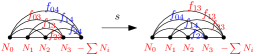
Baldoni–Vergne [BV08, Ex. 16] showed that is integrally equivalent to a flow polytope of a graph with edges and netflow . Recall also that for , then has lattice points and normalized volume . The next result gives a projection between the flow polytope and the Pitman–Stanley polytope. The same projection appears in work of Mészaros–St. Dizier [MSD20, Thm. 4.9, Thm. 4.13, Ex. 4.17] in the context of saturated Newton polytopes and generalied permutahedra333The projection considered by the authors [MSD20] allowed for other graphs other than the complete graph with a restricted netflow depending on ..
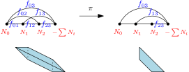
Proposition 7.3.
For and , the projection map , is a surjective map to that preserves lattice points.
Proof.
First we show that . Given in , since each flow in an edge is nonnegative, it suffices to check that for . Note that equals the sum of the flows of the outgoing edges from vertices , i.e. all the flows on edges starting and ending in vertices cancel. Thus
To show the map is onto, we use the fact that is integrally equivalent to and that is a subgraph of the complete graph . See Figure 3(a). ∎
Remark 7.4.
Restricting to the flows to the second to last vertex also gives a projection to the Pitman–Stanley polytope, see Figure 3(b).
Lastly, restricting to the total outgoing flow of each vertex gives a projection to a parallelepiped.
Proposition 7.5.
For , the map , where is a surjective map to the parallelepiped where .
Proof.
From the netflow constraint on vertex we have that
Since , the flow on each edge is at most the netflow , that is . This shows that . It is straightforward to check that this map is onto. ∎
Remark 7.6.
The projections in this section do not give very strong lower bounds. For example for , they give the lower bounds and , respectively.
Acknowledgements
Both authors acknowledge the support of the Natural Sciences and Engineering Research Council of Canada (NSERC), [funding reference number RGPIN-2023-03726 and RGPIN-2024-06246].
Cette recherche a été financée par le Conseil de recherches en sciences naturelles et en génie du Canada (CRSNG), [numéro de référence RGPIN-2023-03726 et RGPIN-2024-06246].
A. H. Morales was also partially supported by NSF grant DMS-2154019 and an FRQNT Team grant number 341288.
We thank the Institut Mittag-Leffler in Djursholm, Sweden and the course of the program on Algebraic and Enumerative Combinatorics in Spring 2020 where the authors met. We thankfully acknowledge the support of the Swedish Research Council under grant no. 2016-06596, and thank Institut Mittag-Leffler for its hospitality. We thank Ivan Balashov, Petter Brändén, Anne Dranowski, Ivan Balashov, Leonid Gurvits, Joel Lewis, Jason O’Neill, Igor Pak, and Martha Yip for helpful comments and suggestions.
References
- [AGH+12] D. Armstrong, A. Garsia, J. Haglund, B. Rhoades, and B. Sagan, Combinatorics of Tesler matrices in the theory of parking functions and diagonal harmonics, J. Comb. 3 (2012), no. 3, 451–494. MR 3029443
- [ALOGV24] Nima Anari, Kuikui Liu, Shayan Oveis Gharan, and Cynthia Vinzant, Log-concave polynomials II: High-dimensional walks and an FPRAS for counting bases of a matroid, Ann. of Math. (2) 199 (2024), no. 1, 259–299. MR 4681146
- [AOG17] Nima Anari and Shayan Oveis Gharan, A generalization of permanent inequalities and applications in counting and optimization, Proceedings of the 49th Annual ACM SIGACT Symposium on Theory of Computing, 2017, pp. 384–396.
- [AOGV21] Nima Anari, Shayan Oveis Gharan, and Cynthia Vinzant, Log-concave polynomials, I: entropy and a deterministic approximation algorithm for counting bases of matroids, Duke Math. J. 170 (2021), no. 16, 3459–3504. MR 4332671
- [Apo99] Tom M Apostol, An elementary view of euler’s summation formula, The American Mathematical Monthly 106 (1999), no. 5, 409–418.
- [Bar07] Alexander Barvinok, Brunn–minkowski inequalities for contingency tables and integer flows, Advances in Mathematics 211 (2007), no. 1, 105–122.
- [Bar09] by same author, Asymptotic estimates for the number of contingency tables, integer flows, and volumes of transportation polytopes, International Mathematics Research Notices 2009 (2009), no. 2, 348–385.
- [Bar10] by same author, What does a random contingency table look like?, Combinatorics, Probability and Computing 19 (2010), no. 4, 517–539.
- [Bar12] by same author, Matrices with prescribed row and column sums, Linear Algebra Appl. 436 (2012), no. 4, 820–844. MR 2890890
- [BBCV06] M. Welleda Baldoni, Matthias Beck, Charles Cochet, and Michèle Vergne, Volume computation for polytopes and partition functions for classical root systems, Discrete Comput. Geom. 35 (2006), no. 4, 551–595. MR 2225674
- [BGDH+19] Carolina Benedetti, Rafael S. González D’León, Christopher R. H. Hanusa, Pamela E. Harris, Apoorva Khare, Alejandro H. Morales, and Martha Yip, A combinatorial model for computing volumes of flow polytopes, Trans. Amer. Math. Soc. 372 (2019), no. 5, 3369–3404. MR 3988614
- [BH10] Alexander Barvinok and JA Hartigan, Maximum entropy gaussian approximations for the number of integer points and volumes of polytopes, Advances in Applied Mathematics 45 (2010), no. 2, 252–289.
- [BH20] P. Brändén and J. Huh, Lorentzian polynomials, Ann. of Math. (2) 192 (2020), no. 3, 821–891.
- [BHH+20] Carolina Benedetti, Christopher RH Hanusa, Pamela E Harris, Alejandro H Morales, and Anthony Simpson, Kostant’s partition function and magic multiplex juggling sequences, Annals of Combinatorics 24 (2020), no. 3, 439–473.
- [BLP23] Petter Brändén, Jonathan Leake, and Igor Pak, Lower bounds for contingency tables via Lorentzian polynomials, Israel J. Math. 253 (2023), no. 1, 43–90. MR 4575403
- [BSDLV04] W. Baldoni-Silva, J. A. De Loera, and M. Vergne, Counting integer flows in networks, Found. Comput. Math. 4 (2004), no. 3, 277–314. MR 2078665
- [BSV04] V. Baldoni-Silva and M. Vergne, Morris identities and the total residue for a system of type , Noncommutative Harmonic Analysis, Springer, 2004, pp. 1–19.
- [BV08] Welleda Baldoni and Michèle Vergne, Kostant partitions functions and flow polytopes, Transform. Groups 13 (2008), no. 3-4, 447–469. MR 2452600
- [CRY00] Clara S. Chan, David P. Robbins, and David S. Yuen, On the volume of a certain polytope, Experiment. Math. 9 (2000), no. 1, 91–99. MR 1758803
- [DLP20] Samuel Dittmer, Hanbaek Lyu, and Igor Pak, Phase transition in random contingency tables with non-uniform margins, Transactions of the American Mathematical Society 373 (2020), no. 12, 8313–8338.
- [EvW04] Richard Ehrenborg and Stephanie van Willigenburg, Enumerative properties of Ferrers graphs, Discrete Comput. Geom. 32 (2004), no. 4, 481–492. MR 2096744
- [GKL24] Leonid Gurvits, Nathan Klein, and Jonathan Leake, From trees to polynomials and back again: New capacity bounds with applications to tsp, 2024.
- [GL21a] Leonid Gurvits and Jonathan Leake, Capacity lower bounds via productization, Proceedings of the 53rd Annual ACM SIGACT Symposium on Theory of Computing, 2021, pp. 847–858.
- [GL21b] by same author, Counting matchings via capacity-preserving operators, Combinatorics, Probability and Computing 30 (2021), no. 6, 956–981.
- [GMP21] Samuel C. Gutekunst, Karola Mészáros, and T. Kyle Petersen, Root cones and the resonance arrangement, Electron. J. Combin. 28 (2021), no. 1, Paper No. 1.12, 39. MR 4245245
- [Gur06a] Leonid Gurvits, Hyperbolic polynomials approach to van der waerden/schrijver-valiant like conjectures: sharper bounds, simpler proofs and algorithmic applications, Proceedings of the thirty-eighth annual ACM symposium on Theory of computing, 2006, pp. 417–426.
- [Gur06b] by same author, The van der waerden conjecture for mixed discriminants, Advances in Mathematics 200 (2006), no. 2, 435–454.
- [Gur09a] by same author, On multivariate newton-like inequalities, Advances in Combinatorial Mathematics: Proceedings of the Waterloo Workshop in Computer Algebra 2008, Springer, 2009, pp. 61–78.
- [Gur09b] by same author, A polynomial-time algorithm to approximate the mixed volume within a simply exponential factor, Discrete & Computational Geometry 41 (2009), 533–555.
- [Gur15] by same author, Boolean matrices with prescribed row/column sums and stable homogeneous polynomials: Combinatorial and algorithmic applications, Information and Computation 240 (2015), 42–55.
- [Hag08] James Haglund, The ,-Catalan numbers and the space of diagonal harmonics, University Lecture Series, vol. 41, American Mathematical Society, Providence, RI, 2008, With an appendix on the combinatorics of Macdonald polynomials. MR 2371044
- [Hag11] J. Haglund, A polynomial expression for the Hilbert series of the quotient ring of diagonal coinvariants, Adv. Math. 227 (2011), no. 5, 2092–2106. MR 2803796
- [hs] David Stewart (https://mathoverflow.net/users/16185/david stewart), Kostant partition function: asymptotics and specifics, MathOverflow, URL:https://mathoverflow.net/q/102647 (version: 2012-07-22).
- [Hum08] James E. Humphreys, Representations of semisimple Lie algebras in the BGG category , Graduate Studies in Mathematics, vol. 94, American Mathematical Society, Providence, RI, 2008. MR 2428237
- [Inc] OEIS Foundation Inc., The On-Line Encyclopedia of Integer Sequences, URL:http://oeis.org.
- [KKOG21] Anna R Karlin, Nathan Klein, and Shayan Oveis Gharan, A (slightly) improved approximation algorithm for metric tsp, Proceedings of the 53rd Annual ACM SIGACT Symposium on Theory of Computing, 2021, pp. 32–45.
- [KMS21] Kabir Kapoor, Karola Mészáros, and Linus Setiabrata, Counting integer points of flow polytopes, Discrete Comput. Geom. 66 (2021), no. 2, 723–736. MR 4292761
- [Lid84] B. V. Lidskiĭ, The Kostant function of the system of roots , Funktsional. Anal. i Prilozhen. 18 (1984), no. 1, 76–77. MR 739099
- [LP22] Hanbaek Lyu and Igor Pak, On the number of contingency tables and the independence heuristic, Bulletin of the London Mathematical Society 54 (2022), no. 1, 242–255.
- [Lus83] George Lusztig, Singularities, character formulas, and a -analog of weight multiplicities, Analysis and topology on singular spaces, II, III (Luminy, 1981), Astérisque, vol. 101-102, Soc. Math. France, Paris, 1983, pp. 208–229. MR 737932
- [Més15] K. Mészáros, Product formulas for volumes of flow polytopes, Proc. Amer. Math. Soc. 143 (2015), no. 3, 937–954.
- [MM19] Karola Mészáros and Alejandro H. Morales, Volumes and Ehrhart polynomials of flow polytopes, Math. Z. 293 (2019), no. 3-4, 1369–1401.
- [MMR17] Karola Mészáros, Alejandro H. Morales, and Brendon Rhoades, The polytope of Tesler matrices, Selecta Math. (N.S.) 23 (2017), no. 1, 425–454.
- [MMS19] K. Mészáros, A. H. Morales, and J. Striker, On flow polytopes, order polytopes, and certain faces of the alternating sign matrix polytope, Discrete Comput. Geom. 62 (2019), no. 1, 128–163. MR 3959924
- [MPP19] Alejandro H. Morales, Igor Pak, and Greta Panova, Asymptotics of principal evaluations of Schubert polynomials for layered permutations, Proc. Amer. Math. Soc. 147 (2019), no. 4, 1377–1389. MR 3910405
- [MS21] Alejandro H. Morales and William Shi, Refinements and Symmetries of the Morris identity for volumes of flow polytopes, Comptes Rendus. Mathématique 359 (2021), no. 7, 823–851 (en).
- [MSD20] Karola Mészáros and Avery St. Dizier, From generalized permutahedra to Grothendieck polynomials via flow polytopes, Algebr. Comb. 3 (2020), no. 5, 1197–1229. MR 4166815
- [O’N15] Jason O’Neill, Exploration of Tesler matrices, 2015, Report for UCLA Department of Mathematics REU.
- [O’N18] by same author, On the poset and asymptotics of Tesler matrices, Electron. J. Combin. 25 (2018), no. 2, Paper No. 2.4, 27. MR 3799422
- [Pos09] Alexander Postnikov, Permutohedra, Associahedra, and Beyond, International Mathematics Research Notices 2009 (2009), no. 6, 1026–1106.
- [Pro90] Robert A. Proctor, New symmetric plane partition identities from invariant theory work of de concini and procesi, European Journal of Combinatorics 11 (1990), no. 3, 289–300.
- [Roc70] R. Tyrrell Rockafellar, Convex analysis, vol. 18, Princeton University Press, 1970.
- [SP02] Richard P. Stanley and Jim Pitman, A polytope related to empirical distributions, plane trees, parking functions, and the associahedron, Discrete Comput. Geom. 27 (2002), no. 4, 603–634.
- [Sta12] Richard P. Stanley, Enumerative combinatorics. Vol. 1, 2 ed., Cambridge Studies in Advanced Mathematics, Cambridge University Press, Cambridge, 2012.
- [Stu95] Bernd Sturmfels, On vector partition functions, J. Combin. Theory Ser. A 72 (1995), no. 2, 302–309. MR 1357776
- [SV17] Damian Straszak and Nisheeth K Vishnoi, Real stable polynomials and matroids: Optimization and counting, Proceedings of the 49th Annual ACM SIGACT Symposium on Theory of Computing, 2017, pp. 370–383.
- [Zei99] Doron Zeilberger, Proof of a conjecture of Chan, Robbins, and Yuen, Orthogonal polynomials: numerical and symbolic algorithms (Leganés, 1998), vol. 9, 1999, pp. 147–148. MR 1749805
- [ZLF17] Yue Zhou, Jia Lu, and Houshan Fu, Leading coefficients of morris type constant term identities, Advances in Applied Mathematics 87 (2017), 24–42.
Appendix A Summary of Basic Bounds and Asymptotics
Throughout the arguments, we use a number of bounds and asymptotic expressions. We compile them here.
Lemma A.1.
For all we have
and
Note that this second bound is redundant with respect to the first bounds.
Proof.
We first prove the upper bound, which is equivalent to
for all . This holds in the limit as , and thus it is sufficient to show that
for all . This holds in the limit as , and thus it is sufficient to show that
for all . This is clear, which proves the desired bound.
We next show that
for all . This clearly holds for , so we will now prove it for . This also holds in the limit as , and thus it is sufficient to show that
for . This holds in the limit as , and thus it is sufficient to show that
for . The denominator is positive, and the quadratic numerator is positive at and negative at . Thus the above inequality holds for , proving the desired bound.
We next show that
for . This holds in the limit as , and thus it is sufficient to show that
for all . This is immediate, which proves the desired bound.
Finally we show that
for all . This holds in the limit at , and thus it is sufficient to show that
for . This holds in the limit as , and thus it is sufficient to show that
for all . This is equivalent to showing that
for all . This holds for , and thus it is sufficient to show that
for all . Since , it is thus sufficient to show that
for all . This is immediate, which proves the desired bound. ∎
Bounds on .
For all we have
| (A.B1) |
Bounds on product of Catalan numbers.
This is from [MS21, Lemma 7.4].
| (A.B2) |
Other asymptotic expression and bounds.
We recall various other asymptotic expressions and bounds. The bounds here are obtainable using simple integration approximation or a standard application of the Euler-Maclaurin formula (Lemma A.2).
| (A.B3) |
| (A.B4) |
| (A.B5) |
| (A.B6) | ||||
| (A.B7) | ||||
Euler-Maclaurin formula.
All of the above bounds can be derived from the Euler-Maclaurin formula, stated below. We make heavy use of Lemma A.3, which is a straightforward corollary.
Lemma A.2 (Euler-Maclaurin formula; e.g. see [Apo99]).
Given integers , a positive odd integer , and a smooth function we have
where is the Bernoulli number and is the Riemann zeta function.
Lemma A.3.
Let be integers, and suppose are real with such that for all . Letting , we have
Proof.
We compute the approximation of the sum , given by Lemma A.2 with and . We have
where
and
and
and
We then have
Combining everything and simplifying yields the result. ∎
Corollary A.4.
For any fixed , we have
where .
Proof.
Using Lemma A.3, we compute (with parameters )
and (with parameters )
and (with parameters )
This gives
Note that a straightforward argument gives the same expression in the limit when . ∎
Appendix B Number of spanning trees
For a tree with vertex set , let . let be the following multivariate sum over spanning trees.
Let be the bipartite graph with edges if .
Theorem B.1 ([EvW04, Thm. 2.1]).
Let with . Let be a bipartite graph with vertices and edges if , then
in particular has spanning trees.
Corollary B.2.
For the graph we have that
in particular has spanning trees.