Quantum Hamilton-Jacobi Theory, Spectral Path Integrals and Exact-WKB
Abstract
We propose a new way to perform path integrals in quantum mechanics by using a quantum version of Hamilton-Jacobi theory. In classical mechanics, Hamilton-Jacobi theory is a powerful formalism, however, its utility is not explored in quantum theory beyond the correspondence principle. The canonical transformation enables one to set the new Hamiltonian to constant or zero, but keeps the information about solution in Hamilton’s characteristic function. To benefit from this in quantum theory, one must work with a formulation in which classical Hamiltonian is used. This uniquely points to phase space path integral. However, the main variable in HJ-formalism is energy, not time. Thus, we are led to consider Fourier transform of path integral, spectral path integral, . This admits a representation in terms of a quantum Hamilton’s characteristic functions for perturbative and non-perturbative periodic orbits, generalizing Gutzwiller’s sum. This results in a path integral derivation of exact quantization conditions, complementary to the exact WKB analysis of differential equations. We apply these to generic symmetric multi-well potential problems and point out some new instanton effects, e.g., the level splitting is generically a multi-instanton effect, unlike double-well.
”I like to find new things in old things.” Michael Berry
1 Introduction
Classical mechanics is to quantum mechanics what geometric optics is to wave optics. In the cleanest form of the correspondence principle, Hamilton-Jacobi formulation of classical mechanics plays a prominent role. Let us briefly remind its well-known version. For a time-independent Hamiltonian, using , Schrödinger equation becomes the non-linear Riccati equation,
| (1) |
For , (1) is an exact representation of the Schrödinger equation. For , (1) is an exact representation of classical mechanics, it is the equation for Hamilton’s characteristic function , which carries the same information as Newtonian, Lagrangian, or Hamiltonian formulation. At infinitesimal , in (1) should be viewed as the quantum generalization of the Hamilton characteristic function.
Riccati equation is the starting point of the exact WKB formalism dillinger_resurgence_1993 ; DDP2 ; balian_discrepancies_1978 ; Voros1983 ; Silverstone ; aoki1995algebraic ; AKT1 ; sueishi_exact-wkb_2020 . It can be converted to a recursive equation the solution of which is given in terms of asymptotic series in . Exact-WKB is the study of a differential equation in complexified coordinate space () by using resurgence theory Ec1 ; sauzin2014introduction , and Stokes graphs. Classical data about the potential dictates the Stokes graph, and demanding monodromy free condition from the WKB-wave function leads to the exact quantization conditions.
Of course, this is a very elegant formalism but it is also clear that this line of reasoning does not take advantage of the full Hamilton-Jacobi theory. In classical mechanics, the power of Hamilton-Jacobi theory stems from the ability to select a canonical transformation to new coordinates which are either constants or cyclic. In particular, one can even choose a generating function such that the new Hamiltonian is zero, or a constant ,
| (2) |
The whole solution of the classical system is in the reduced action, . What is the implication/benefit of classical canonical transformations in the context of quantum mechanics?
To explore the answer to this question in quantum theory, we must work in a formulation of quantum mechanics in which classical Hamiltonian enters the story. This uniquely points us to work with the phase space path integral. One may be tempted to think that one should work with the phase space path integral in the standard form:
| (3) |
The trace implies that we need to integrate over paths satisfying periodic boundary conditions , returning to themselves at fixed time . Such paths can be rather wild, unearthly, and the energy can take any value, even infinity so long as it is periodic.111The same is also true in configuration space path integral with uses classical Lagrangian, . It also does not matter if we are considering Minkowski time or Euclidean time, where the latter corresponds to thermal partition function However, the key player in classical Hamilton-Jacobi theory, Hamilton’s characteristic function is a function of . It would be more natural to work with all paths not at a fixed time , but at a fixed energy .
In some way, we would like to perform phase space path integrals not at a fixed (where can take arbitrarily large values), but at fixed (where can take arbitrarily large values). Therefore, it is more natural to work with the Fourier transform of the path integral, which is a function of .
| (4) |
This is nothing but the resolvent for the original Hamiltonian operator , and it is simply related to spectral determinant
| (5) |
In our context, it is more natural to view both of these as phase space path integrals which are functions of , i.e., spectral path integrals, and we will use this terminology interchangeably with resolvent and spectral determinant.
It is the spectral path integral (4), not the original (124), that allows us to explore the implication of the Hamilton-Jacobi formalism for the path integrals in phase space. Physically, the main advantage of is that the set of paths that contribute path integral is discrete infinity, and countable. This is unlike the one that enters in configurations space path integral , which is continuous infinity.
In essence, we generalize the classical canonical transformations of the Hamilton-Jacobi to a quantum canonical transformation in the context of phase space path integral. The classical reduced actions are promoted to quantum ones:
| (6) |
In classical mechanics, only the classically allowed cycles contribute to the equations of motions and dynamics. What is the set of cycles that enter the quantum theory? 222This question, in configuration space path integral formulation, is equivalent to which saddles contribute to the path integral? What is the role of generic complex saddles?
It turns out this question has a sharp answer. It is given in terms of what we will refer to as vanishing cycles. These are the cycles for which as is varied, two or more turning points coalesce at some critical . The critical are associated with separatrices in classical mechanics of the potential problems for and . The classically allowed vanishing cycles will be called perturbative (or classical) cycles , and classically forbidden vanishing cycles will be called non-perturbative (or dual) cycles .
| (7) |
The spectral path integrals will be expressed in terms of quantum generalizations of Hamilton’s characteristic functions on these cycles, and , also called Voros multipliers. There are important advantages gained from the spectral path integral.
-
•
Upon Hamilton-Jacobi canonical transformation, the spectral phase space path integral becomes a discrete sum involving the quantum version of the reduced actions associated with independent vanishing cycles, .
-
•
The discrete sums in terms of vanishing cycles can be performed analytically. The remarkable fact is that the path integral sum produces the exact quantization conditions that is obtained in the exact-WKB analysis, by the study of differential equations in complex domains. Our construction, based on quantum Hamilton-Jacobi, provides a streamlined derivation of the proposal in sueishi_exact-wkb_2020 ; sueishi_exact-wkb_2021 ; kamata_exact_2023 .
-
•
The spectral determinant and spectral partition function can be written as
(8) where subscripts denote the sums over perturbative and non-perturbative vanishing cycles, respectively. The zeros of gives the spectrum of quantum theory. This shows that the quantum spectrum of the theory can be explained in terms of properties of the classical cycles, with both p and np cycles included, answering Gutzwiller’s fundamental question gutzwiller_periodic_1971 ; gutzwiller_periodic_1971-1 . (See also Witten:2010zr ).
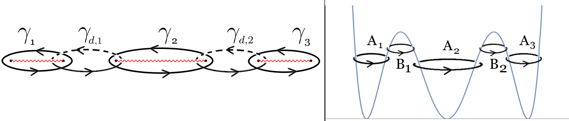
As an example, the spectral partition function for a 4-well potential problem reduces to the discrete sum over the orbits shown in Fig. 1. The first line is the sum over perturbative vanishing cycles. The sum gives . The second and third are the sum over the nonperturbative cycles and they add up to . gives the quantum spectrum of the theory.
Relation to other works
The central theme of the exact WKB analysis is the study of differential equations in complex domains, by using asymptotic analysis, resurgence and Stokes graphs. The philosophy of this work is complementary. It is the study of the spectral phase space path integral by using the (quantum) Hamilton-Jacobi formalism. Although methods are different, both yield exact quantization conditions. There is ultimately an overlap of the two formalisms, because exact quantization conditions are expressed in terms of Hamilton’s characteristic functions (reduced actions or Voros symbols). However, we believe the path integration demystifies the origins of the quantization conditions, as sum over p/np periodic orbits, while in the exact WKB, the same condition arises from the normalizability of the analytically continued WKB wave function as . The remarkable fact is that both of these expressions are given in terms of for the p/np cycles in the problem.
Below, we mention some important developments on the exact WKB and quantization conditions. Exact quantization condition capturing all multi-instanton effects was conjectured by Zinn-Justin:2004vcw ; Zinn-Justin:2004qzw ; jentschura_multi-instantons_2010 ; jentschura_multi-instantons_2011 as generalized Bohr-Sommerfeld quantization, which is based based on classically allowed (P) and classically forbidden (NP) cycles. The conjecture was proven dillinger_resurgence_1993 ; DDP2 following the work of balian_discrepancies_1978 ; Voros1983 ; Silverstone , and using resurgence theory Ec1 in some special cases.
Another important result is derived for genus-1 potential problems. The full non-perturbative expression for energy eigenvalues, containing all orders of perturbative and non-perturbative terms, may be generated directly from the perturbative expansion about the perturbative vacuum Dunne:2013ada ; Dunne:2014bca ; Alvarez3 ; Cavusoglu:2023bai . This fact is quite remarkable and its generalization to higher genus potentials is an open problem.
The WKB connection formulae, together with the condition of monodromy-free wavefunction lead one to find the spectral determinant of a quantum mechanical system, hence the exact quantization condition for general -well systems. Consequently, an explicit connection between the exact WKB theory and the path integral was made in sueishi_exact-wkb_2020 ; sueishi_exact-wkb_2021 ; kamata_exact_2023 , also the relation to the pioneering work of Gutzwiller gutzwiller_periodic_1971 ; gutzwiller_periodic_1971-1 is pointed out.
The sum over vanishing cycles gives a generalization of the Gutzwiller summation formula. The Gutzwiller summation formula in its original form is phrased in terms of cycles that enter classical mechanics (prime periodic orbits) gutzwiller_periodic_1971 ; gutzwiller_periodic_1971-1 ; MVBerry_1977 . In quantum mechanical path integral for general potential problems, vanishing cycles also include non-perturbative (tunneling or instanton) cycles. A proposal that Gutzwiller’s approximate trace formula can be turned into an exact relation in terms of Voros symbols of all cycles was made in Ref.Nekrasov:2018pqq . For other recent developments in semi-classics and exact WKB in quantum mechanical systems, see Grassi:2014cla ; Basar:2013eka ; Gahramanov:2015yxk ; Behtash:2015kna ; Dunne:2016jsr ; Dunne:2016qix ; Kozcaz:2016wvy ; Basar:2017hpr ; Behtash:2015loa ; Codesido_2018 ; Behtash:2018voa ; Sulejmanpasic:2016fwr ; Dunne:2020gtk ; Iwaki1 ; Kamata:2023opn ; Kamata:2024tyb ; Bucciotti:2023trp . For the relation between supersymmetric gauge theory and exact WKB, seeGaiotto:2009hg ; Kashani-Poor:2015pca ; Basar:2015xna ; Ashok:2016yxz ; Yan:2020kkb ; Hollands:2019wbr ; Grassi:2021wpw ; Grassi:2022zuk
2 Spectral Determinant as Spectral (Phase Space) Path Integral
We first remind briefly of the relation between the resolvent, spectral determinant, and phase space path integral. These are quantities that possess complete information about the energy spectrum of the quantum system. As in muratore-ginanneschi_path_2003 ; Schulman:1981vu , we start with the usual definition of the propagator
| (9) |
and for . The propagator (9) works as the kernel of the Schrödinger equation,
| (10) |
Since we are only considering forward propagation in time, we can rewrite as
| (11) |
where . Assuming that the corresponding Hilbert space is spanned by a complete set of energy eigenstates of the Hamiltonian operator , we can express the propagator as
| (12) |
The propagator has information on the spectrum , and is a function of time .
It is more convenient to define a spectral function as a function of energy via the Fourier transform
| (13) | ||||
| (14) |
In particular, when we use path integrals, the Fourier transform will allow us to work with paths with fixed , rather than paths with fixed . This step will also be crucial in carrying over Hamilton-Jacobi to quantum theory. Using (13), we have
| (15) | ||||
| (16) |
To obtain the second line, we performed the integration over by adding a small imaginary complex term for convergence, and then let in the final result. This is the resolvent associated with the Hamiltonian operator, and satisfies:
| (17) |
Therefore, one maps the energy spectrum of the system to the poles of the trace of the resolvent
| (18) |
A related important object that encodes spectral data is the Fredholm determinant
| (19) |
such that is the quantization condition for a system with Hamiltonian . Observe that the resolvent and the Fredholm determinant are related to each other as
| (20) |
Using the inverse Fourier/Laplace transform of one gets
| (21) |
since is nothing but the trace of the propagator
| (22) |
where periodic refers to . Putting everything back into (20), one gets the relationship
| (23) |
At first sight, this equation is easy to derive and looks pretty simple. It is the relation between the spectral resolvent and phase space in path integral. In what follows, we present a formulation that represents path integral in terms of cycles in phase space.
2.1 Classical and Quantum Canonical Transformation
Classical Hamilton-Jacobi transformation: We first discuss the Hamilton-Jacobi formalism in classical mechanics, and next, we discuss its implementation to quantum theory. For any classical system, one can consider a canonical transformation defined by the type-2 generating function , such that
| (24) |
One can choose the action to be the generating function up to a constant
| (25) |
then we see that the new Hamiltonian in terms of the new coordinates is identically zero,
| (26) |
Therefore, the new coordinates are constants of motion, i.e., their equations of motion are trivial:
| (27) |
Writing everything in terms of the old coordinates, (26) gives the Hamilton-Jacobi equation
| (28) |
If one considers a system with a time-independent Hamiltonian, we can separate the variables of as
| (29) |
Here, the time-independent term, is called Hamilton’s characteristic function or reduced action. By substituting (29) into Hamilton-Jacobi equation (28), we obtain the equation for .
| (30) |
which defines the classical trajectories as the level sets of the Hamiltonian. One can choose the new coordinates and momenta as the initial time and the energy , both being the constants of motion. Then, (30) implies the form of the old momentum trajectories to be
| (31) |
Quantum Hamilton-Jacobi transformation: To carry out a similar implementation to quantum mechanics, we need to promote the action to be the ”quantum” action. Assume that there exists a quantum generating function that results in the canonical transformation
| (32) |
For systems with time-independent Hamiltonian, we may again take the generating function to be the quantum action with separated variables
| (33) |
However, this time the trajectories satisfy the quantum version of the Hamilton-Jacobi equation which is a partial differential (Riccati) equation
| (34) |
equivalent to the Schrödinger equation. This implicitly defines the quantum momentum function as a function of and satisfying
| (35) |
Everything defined above is equivalent to classical mechanics in the limit . It then follows from (24) that the new coordinates are defined as
| (36) | ||||
| (37) |
We have chosen our new coordinates to be the constants of motion of the classical trajectories plus their quantum corrections. For periodic trajectories, the quantum variables and are also constants of motion. The coordinate is on the same footing as a time coordinate on the trajectory. For a canonical transformation, the jacobian for the path integral is just 1, i.e.,
| (38) |
The action in the exponent transforms as (for periodic boundary conditions)
| (39) |
where
| (40) |
is the quantum-reduced action for periodic paths which allows us to define its quantum period
| (41) |
In the functional integral (124), we are performing a sum over arbitrary periodic paths in phase space. Now that we transformed the phase space into the coordinates , we can alternatively talk about periodic paths in the space, and perform a path integral therein. This is possible for arbitrary periodic paths and we treat as its parameterizations. We are now in a position to take the path integral for ,
| (42) | ||||
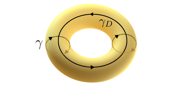
where are the integration cycles defined as the linear combinations of the connected fundamental periods on an -torus
| (43) |
and is the period of a prime periodic orbit, generating . The factor is called Maslov index maslov1972theory . In Bohr-Sommerfeld quantization, this accounts for the extra phase corrections to quantization condition found originally by Einstein, Brillouin, and Keller. For a simple derivation, see sueishi_exact-wkb_2020 . Here, we treat as a flow parameter for the paths in space. The functions have all the terms of the quantum reduced action in orders of evaluated at each initial point of . After taking integrals, the energies of the paths are set to a level set . Quantum Hamilton-Jacobi equation relates the quantum corrections in the reduced action to the classical reduced action.
| (44) |
Once is set to , the path integral becomes a sum over prime periodic orbits . These include perturbative cycles (classically allowed cycles) and non-perturbative (classically forbidden) cycles. In the standard path integral language, non-perturbative cycles are associated with instantons and other tunneling-related phenomena. This provides a generalization of the Gutzwiller’s sum over the classical prime periodic orbits now including both real and complex orbits. Each of these cycles encircles a pair of classical real turning points, in the classically allowed regions as well as classically forbidden regions. Both of these enter naturally into the path integral. The only difference is in their weight factors. is oscillatory for classically allowed cycles and exponentially small for the classically forbidden ones. More details about the prime periodic orbits are given in the appendix.
Lastly, recall that the amount of time past for orbits can only be an integer multiple of the period defined as in (41). Therefore, the integration turns into a discrete sum over periods of the corresponding orbit. Finally, we arrive at the main result.
| (45) |
with
| (46) |
where factor is related to the phase change of the exponent after circling the turning points -times. When there are no turning points, no phase change occurs. The form of the non-perturbative spectral path integral is more complicated since for non-perturbative trajectories, one needs to consider all possible periodic paths that exhibit tunneling. We will discuss and give its explicit form momentarily.
We see that at fixed , the path integration is now a sum over all possible periods. Since is fixed, it can only occur over the same minimal path, tracing it infinitely many times, but its period can only be an integer multiple of the minimal orbit’s period. Using the relationship between the spectral determinant and the resolvent (23), we can write the logarithm of the spectral determinant schematically as
| (47) |
where we have used the fact that the quantum periods are given by the energy derivative of the quantum reduced action (41). The normalization factor, is equal to one for classically allowed cycles. Classically forbidden cycles requires more care. Even for just one classically forbidden cycle, there are infinitely many possible perturbative cycles that can dress it up. This summation generates the factors for the NP-cycles, where dressing is a function of the reduced actions of the adjacent perturbative cycles . We will give a precise derivation of this factor for most generic cases we examine.
or obtained from the phase space path integral, as a sum over generalized prime periodic orbits, turns out to be equivalent to the result of the exact WKB analysis, which is the study of differential equation in complexified coordinates, using Stokes graphs, resurgence and connection formula. In certain sense, our construction provides a physical interpretation of the exact quantization conditions from path integral perspective. It is a consequence of the summation over all periodic cycles entering the level set of the potential problem .
Lastly, let us justify our assumption about the canonical transformation that results in the ”quantum” reduced action where we only use the classical trajectories as the integration cycles. Once the Riccati equation is solved, say, as an asymptotic expansion in , one can show that the resulting differential one-forms live in the same cohomology space as the classical action differential with a common . This implies that each differential one form in higher orders of can be generated by acting on the classical action differential with a differential operator in , called the Picard-Fuchs differential operators. More detail on this is given in the appendix.
3 Building The Summation: Simplest to generic potential problems
Let us start with the simple harmonic oscillator.
| (48) |
For each energy level , we only have one topologically distinct cycle. This is just the reflection of the fact that this system has only one vanishing cycle, as is varied, the two turning points coalesce only at . Therefore, the only periodic paths that contribute to the path integral are those that are multiple integers of the classical orbit associated with the energy . Hence, the path integral turns into a discrete summation over positive integers and the spectral determinant becomes
| (49) |
The area in phase space circulated by at energy level is just . The spectrum of the quantum theory are zeros of the spectral determinant, and hence, the quantization is obtained by setting
| (50) |
which is nothing but the Bohr-Sommerfeld quantization condition:
| (51) |
3.1 Double Well
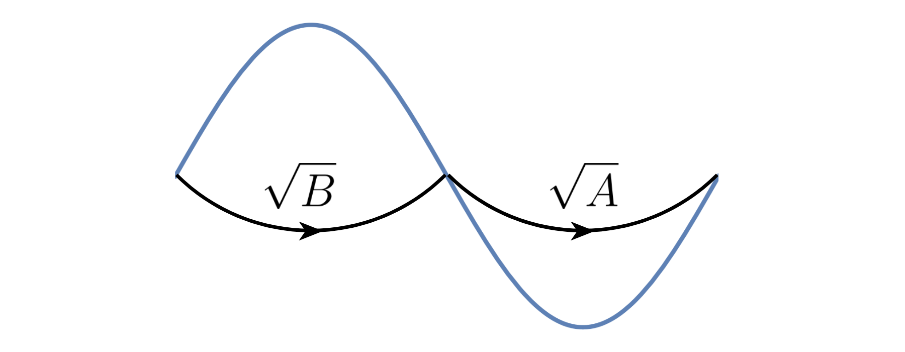
To understand how the path integral summation should be carried out with systems that have instantons or bions, we first use a simple and important example, symmetric and asymmetric double well system. First, let us assume that the frequency of each well is different, namely, and , with , and being the minima of the potential. There are two perturbative vanishing cycles and one nonperturbative vanishing cycle. We define the exponential of the quantum version of Hamilton’s characteristic function over periodic cycles, called Voros symbols in exact WKB as
| (52) |
For now, we treat the quantum-reduced actions to be analytic functions of in the region , where is the local maximum (barrier top). The cycles are defined by analytically continuing in the complex -plane with , encircling the classical turning points of the level set . Here cycles vanish at and vanishes at when the encircled turning points coalesce. In the phase space of classical mechanics, the level set defines the separatrix.
One may think of ’s as the Borel resummed version of their asymptotic series in as in (44). This brings about a Stokes phenomenon and an imaginary ambiguity in the analytical continuation between different choices of and . Two choices are related by the monodromy properties of the moduli space via the transformation . This amounts to going to a proper sheet and mapping one choice to the other. Also, we’ll see that it maps one spectral determinant when to the other with . Without loss of generality, we will work with . This will only change the factor in front of the nonperturbative transmonomial . One can show that the imaginary ambiguity cancellation occurs after the medianization of the Voros symbols but we won’t pursue that direction dillinger_resurgence_1993 ; Aniceto:2013fka ; sueishi_exact-wkb_2020 .
It is straightforward to identify the perturbative paths, they are just integer multiples of the topologically distinct cycles . Hence any other perturbative trajectory can be generated by the transmonomial
| (53) |
which gives the perturbative part of the spectral path integral for ,
| (54) | ||||
Let us now try to identify the nonperturbative transmonomial by considering periodic paths that exhibit tunneling. One may be tempted to think that a similar summation would do the job. That is, any nonperturbative path is generated as an integer multiple of .
| (55) |
However, this is incorrect. The particle can tunnel through from the left well to the right one and oscillate there -times, then tunnel back. This is also a distinct periodic path for each . Therefore, in general, we need to consider all possible oscillations in each well together with tunneling from left to right and vice versa. Then the path integration (summation) should be over all these paths. Ultimately, their combinations will appear in the powers of describing all possible -periodic tunneling events with their binomial weights. This might sound cumbersome, but you’ll see that they repackage themselves quite nicely. Consider the following summation describing the transmonomial with all possible paths with a single periodic tunneling event.
| (56) |
Here, notice the minus sign in the exponent of . This is because, after one tunneling event from left to right, we change Riemann sheets by going through the branch cut. We go back to the same sheet after tunneling to the left, whence no minus sign for . We formally carry out this summation over ’s
| (57) |
It is now easy to write down the nonpertubative spectral path integral for the determinant,
| (58) | ||||
Lastly, we arrive at the quantization condition , from the fact that
| (59) |
one gets finds the exact quantization condition to be
| (60) |
This is the same result as one would get from the WKB analysis by demanding normalazibility of the WKB wave function.
Had we started with , one had to choose in the transmonomial (57) instead, and would end up with
| (61) |
This is a mere choice of our definitions of the cycles in the first sheet. The two cases are related to each other via the action of the monodromy around . To see the effect of the monodromy of , consider the transformation . The quantum momentum function is invariant under this transformation but the dual (co)vanishing cycle is not. The dual vanishing cycle transforms according to the Picard-Lefschetz formula
| (62) |
where the perturbative vanishing cycles are invariant under the action of the monodromy transformation (Fig.[4]).
Thus, nonperturbative transmonomial, defined for , transforms as
| (63) |
which is the same transmonomial defined for .
We see that the nonperturbative transmonomial comes dressed up with the spectral determinants of the perturbative orbits alternating in separate sheets connected via tunneling. These are the factors mentioned in (47).
For a symmetric double-well potential, the quantization condition becomes
| (64) |
Application: Apart from being a quantitatively excellent tool, the quantization condition is also a qualitatively useful tool. The leading order non-perturbative contribution to symmetric and asymmetric (classically degenerate) double well potentials are of different nature Miller , as it can be seen by solving quantization conditions. One finds, the leading non-perturbative contribution to the energy spectrum as:
| (65) |
For a symmetric double-well potential, it is well-known that the leading non-perturbative effect is level splitting, of order , which is due to an instanton. For an asymmetric, and classically degenerate double-well potential, with , despite the fact that instanton is a finite action saddle, the instanton contribution vanishes. As explained in detail in §.4, the fluctuation determinant is infinite and this renders the instanton contribution zero. The leading order non-perturbative contribution to vacuum energy is of order , the bion (or correlated instanton-anti-instanton effect). The determinant of fluctuation operator for this 2-event is finite, and hence it contributes to the spectrum. For related subtle non-perturbative phenomena and detailed explanations, see §.4.
3.2 Symmetric Triple Well
Now that we have gained a sense of how the summation of the prime periodic orbits should be carried out when the system includes nonperturbative effects due to instantons, we are ready to apply our prescription to a more complicated system such as the symmetric triple well potential
| (66) |
In this case, There are three perturbative vanishing cycles and two nonperturbative vanishing cycles. Defining each Voros symbol as
| (67) |
For the symmetric triple-well,
| (68) |
so we’ll use and as a convention in our notation.
Now, our objective is to identify the minimal (prime) periodic orbits that represent the tunneling process from one well to the other. As shown in Fig. [6], one can see that there are 3 such minimal periodic orbits. One can mix these minimal periodic orbits to form other periodic orbits that include more than one tunneling process. However, these are not minimal and will be formed in the higher orders of the summation procedure via binomial combinations of the minimal periodic orbits. Hence, we deduce that the nonperturbative transmonomial that spans all of these paths should be a linear combination of the Voros symbols of these 3 minimal orbits,
| (69) |
Therefore, the spectral path integral will give the following sum for the spectral determinant
| (70) | ||||
| (71) | ||||
| (72) |
From this, one can find the exact quantization condition for the system to be
| (73) |
as promised in the exact WKB connection formula. For explicit computations of , and spectral quantities, see kamata_exact_2023 ; Dunne:2020gtk .
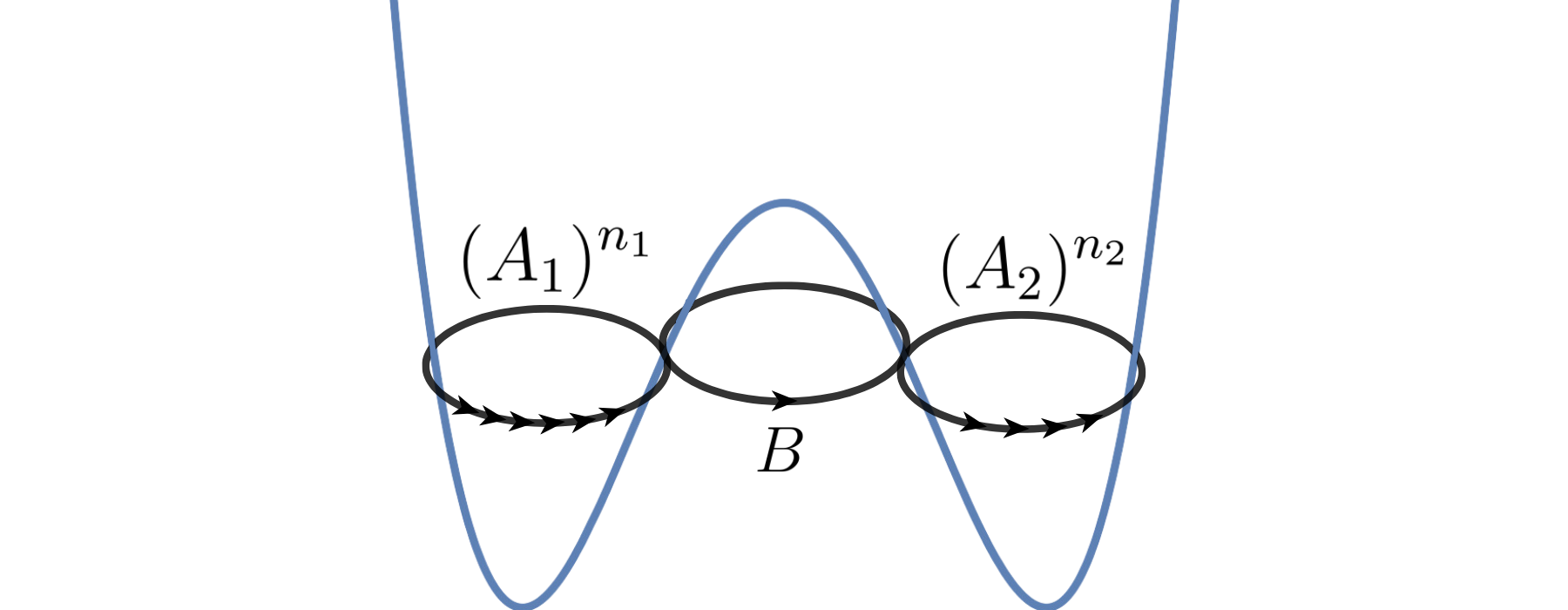
3.3 General N-ple Well
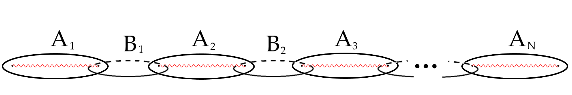
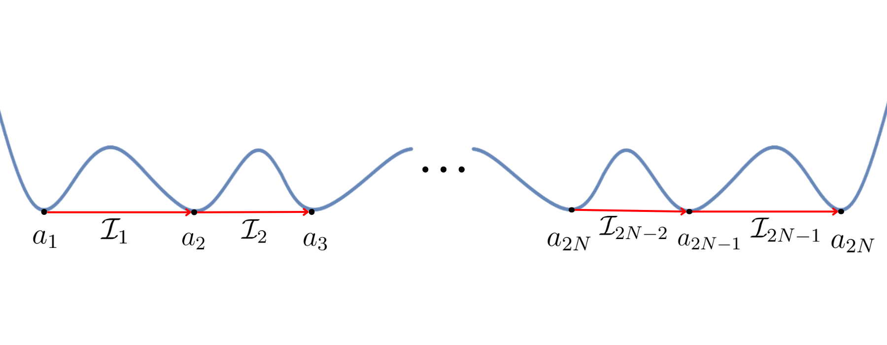
Now that we have had enough exercise, we can give a general formula for the spectral path integral, hence the spectral determinant, of a general system with wells. Define the perturbative Voros symbols for each well and the nonperturbative Voros symbols connecting consecutive wells as
| (74) |
where for ’s and for ’s. The orbits can be pictorially represented as shown in Fig.[7].
We have already shown that the spectral path integral will be decomposed into its perturbative and nonperturbative parts, which will translate into the same decomposition for the logarithm of the spectral determinant
| (75) |
so our task is to determine the nonperturbative transmonomial. From our previous experience, we deduce that it should be written as
| (76) |
| (77) |
Where the symbols represent the alternating signs of the consecutive Voros symbols’ exponent.
| (78) |
Hence we have the spectral determinant for a general system with -wells
| (79) | ||||
| (80) | ||||
| (81) |
is the exact quantization condition for the system which agrees with the known form in sueishi_exact-wkb_2020 .
3.4 Quantum Mechanics on
Let us now apply our knowledge to quantum mechanical systems with periodic potentials obeying
| (82) |
By Bloch’s theorem, the wavefunction of a system with periodic potential attains the form
| (83) |
with , so that it satisfies
| (84) |
The spectra of the system consist of bands whose states are labeled by the continuous Bloch momenta . Upon gauging the translation symmetry, we make the physical identification of with . Hence, the space is compactified to a circle, that is, . Therefore, we can introduce a theta-angle, such that one has the relationship of the wavefunctions
| (85) |
where we have set the lattice spacing . We need to account for this fact in our formulation of the spectral determinant.
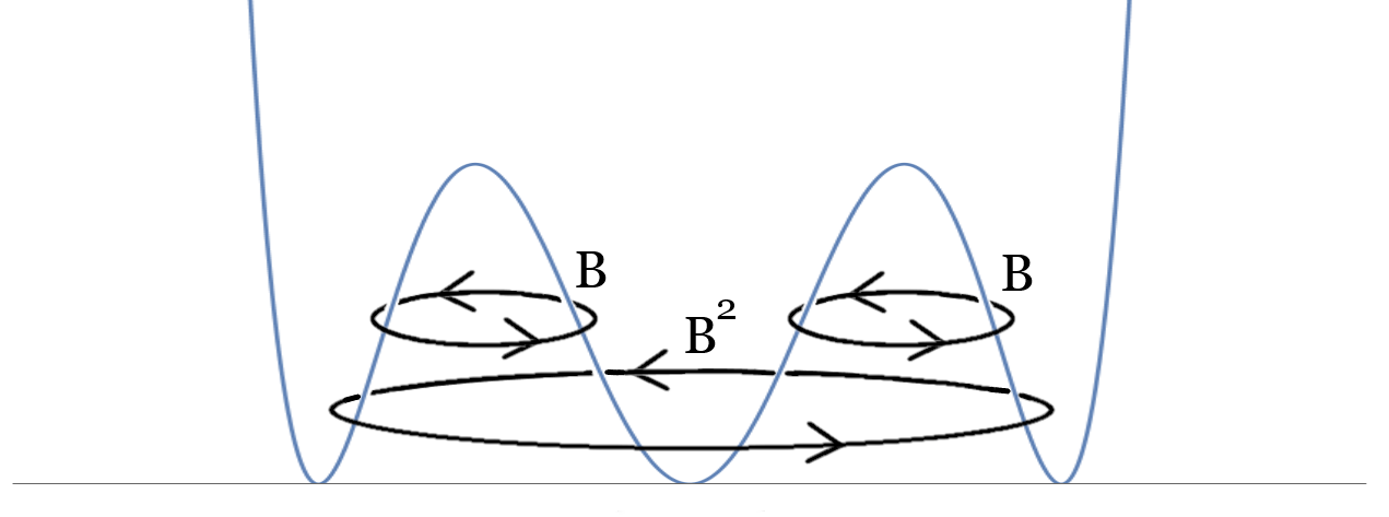
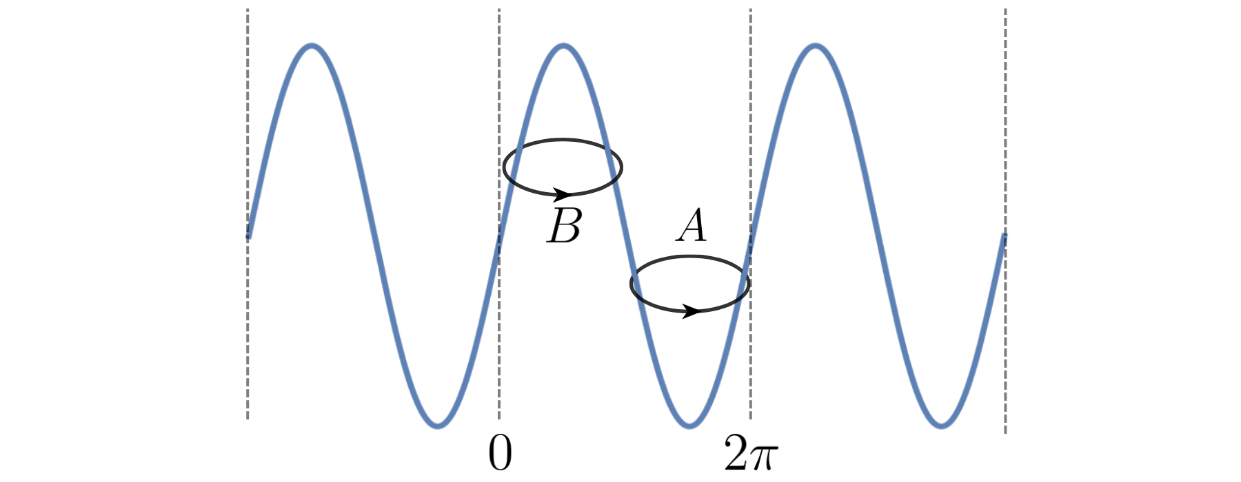
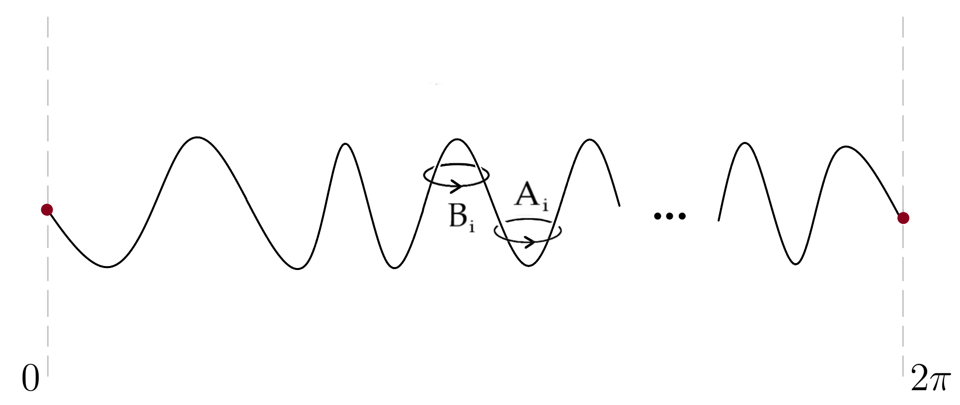
minima in fundamental domain: For simplicity and demonstration purposes, assume that the potential has only one minimum and one maximum in the fundamental domain as shown in Fig.[8]. This corresponds to having one classical and one dual cycle with the corresponding Voros multipliers as usual,
| (86) |
To do the summation over the prime periodic orbits, we need to account for the fact the points are physically identified. Therefore, on top of the usual perturbative and nonperturbative minimal transmonomials
| (87) |
we also have the topological transmonomial that will contribute to the nonperturbative minimal transmonomial
| (88) |
corresponding to another prime periodic orbit as shown in Fig.[9]. This can be observed from the fact that
| (89) |
where is the cycle encircling the turning points and in the complex q-plane. The minus sign in equation (88) is from the fact that we encounter 2 turning points along the trajectory.
Hence, we can write down the spectral determinant via spectral path integral (summation)
| (90) | ||||
It then implies that
| (91) |
is the exact quantization condition for the system with a periodic potential having one minimum and one maximum on the fundamental domain , sueishi_exact-wkb_2021 .
Observe that in the case of , the quantization condition reduces that of a free particle () on a circle, say, with radius ,
| (92) | ||||
| (93) |
The integral in the exponent is written as
| (94) |
then the quantization condition implies that
| (95) |
Both conditions are equivalent for integer . Hence, one finds the energy levels to be
| (96) |
where .
minima in fundamental domain: The generalization to a periodic potential with distinct minima and distinct maxima in the fundamental domain is straightforward as in the case of -ple well system. Again, we define each distinct Voros symbols
| (97) |
with . The spectral path integral as a sum over prime periodic orbits will give the form of the spectral determinant to be
| (98) |
Observe that there is only one such topological transmonomial connecting the physically identified points to as shown in Fig.[10]. Hence, we identify each transmonomial as
| (99) | ||||
| (100) | ||||
| (101) |
where are topologically identified. Hence, we can write the spectral determinant as
| (102) |
is the quantization condition for a system with periodic potential with distinct minima and distinct maxima in the fundamental domain .
4 Strange Instanton Effects
The exact quantization condition can be used both as a qualitative tool as well as a quantitative tool to learn about the dynamics of quantum mechanical systems. In this section, we use it as a quantitative tool to deduce some strange sounding non-perturbative effects. Trying to translate the implications of these effects to more standard instanton language teaches us some valuable lessons about instantons, multi-instantons and their role in dynamics.
In particular, we will show that in generic multi-well systems, despite the fact that instantons are exact saddles, they do not contribute to the energy spectrum at leading order. The leading NP contributions are from critical points at infinity, correlated two-events or other clusters of the instantons. The leading order instanton contributions in double-well and periodic potentials seems to be an exception, rather than the rule. And we would like to explain this within this section.
Consider a generic -well potential with reflection symmetry.
| (103) |
We assume that the frequencies are unequal, except the ones enforced by symmetry,
| (104) |
Clearly, there exist instanton solutions interpolating between adjacent vacua. Let us enumerate them as
| (105) |
where denotes instanton interpolating from to . We would like to understand their role in non-perturbative dynamics by using exact quantization conditions as a guiding tool. The exact quantization condition produces some results that may seem exotic from the instanton point of view.
We would like to determine the level splittings between the perturbatively degenerate lowest states in each well, , for . By solving exact quantization conditions, we find the leading order level splitting to be the following:
| (106) | ||||
| (107) | ||||
| (108) | ||||
| (109) | ||||
In other words, the splitting of the degeneracy between is a -instanton effect. The splitting between is a - instanton effect. Finally, the splitting between is a -instanton effect.
Despite the fact that instantons exist as saddles, the leading splitting between and is - instanton effect! Thus, we learn that except for adjacent middle minima, the level splitting is never a 1-instanton effect. In this sense, the double-well potential is an exceptional case. This said, it is worthwhile emphasizing that (109) is not generically the leading non-perturbative effect. There are much larger NP effects but they do not lead to level splitting, rather they lead to the overall shift of the energy eigenvalue. For example, let us express various contributions to . We find
| (110) | |||
| (111) |
The 2-instanton , 4-instanton, …, -instanton effects are also present, but they do not lead to level splitting. The leading order level splitting comes from instantons. Eq.(111) comes from the solution of exact quantization condition. How do we understand it from the standard instanton analysis of path integral? Why do exact saddles do not contribute, but their clusters do?
Instantons are solution for the non-linear equations:333Our convention for instantons is shown in Fig. 11. They are tunneling from to , and is always an increasing function. If is the solution for , then the configuration must be the solution of , and this continues in this alternating manner. This alternation is due to the fact that our left hand side is increasing in our convention. Yet, switches signs at all .
| (112) |
It is easy to solve for the inverse function , but the function is cumbersome when the number of wells is greater than four. The expression for is
| (113) |
The solutions are exact, they have finite action, and one would naively expect a contribution to the spectrum of the form from these configurations.
However, the full instanton amplitude also includes the determinant of the fluctuation operator around the instanton solution. The amplitude is of the form
| (114) |
The prime indicates that the zero mode is omitted from the determinant. It must be integrated over exactly, with a measure given by the Jacobian factor . is the normalization by the free fluctuation operator around the perturbative vacuum, present to regularize the determinant. The crucial property of the generic fluctuation operator is its asymmetry. This generates the difference with respect to double-well and periodic potential examples, for which is symmetric. The asymmetry of the fluctuation operator implies that its determinant remains infinite even after regularization.
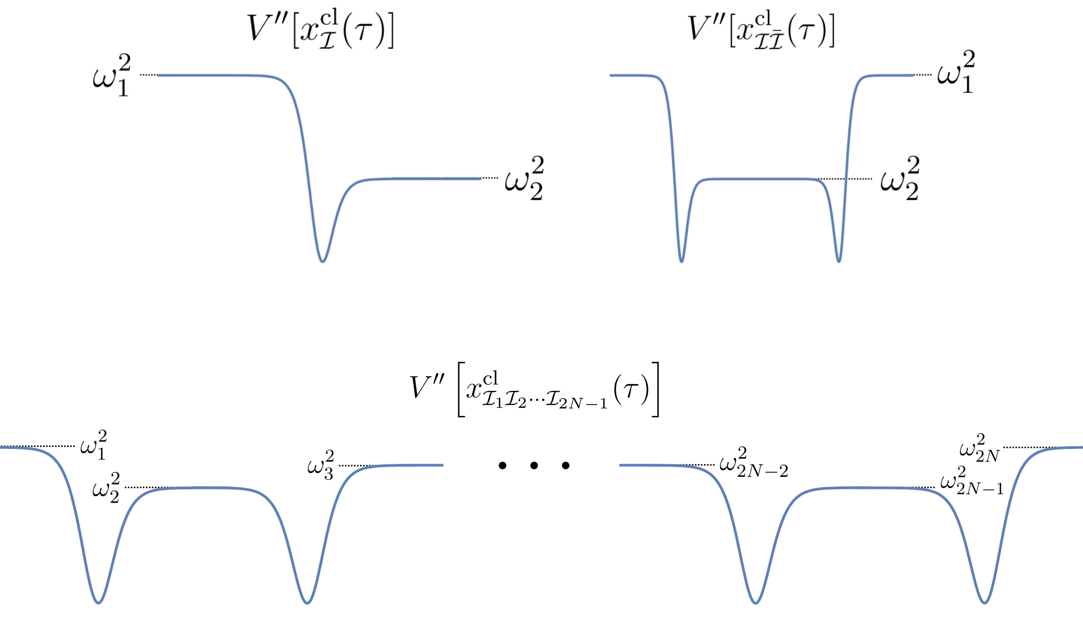
To determine the determinant of fluctuation operator, we need the asymptotic profile of the instanton solution at least asymptotically, As , and , . Let us write and at two asymptotes. It is easy to determine both , as well as . We find
| (117) | ||||
| (120) |
as we can derive from the exact inverse-solution (113). We do not need the full form of the fluctuation operator to show the vanishing of the instanton, and non-vanishing of bions, and certain other clusters. The crucial point here, compared to the instantons in double-well potential, is the generic asymmetry of as , shown in Fig.12. Because of this, the regularized determinant still remains infinite:
| (121) |
Hence, the instanton amplitude in this system is ironically zero despite the fact that instanton configuration is finite action.
| (122) |
On the other hand, if we consider a bion , which is not an exact solution due to interactions between the instantons, has a symmetric profile: as , as , as shown in Fig.12. The fluctuation operator is symmetric and the prefactor is finite.
Similarly, for the correlated events , the fluctuation operators are symmetric and finite as well, see Fig.12. As a result, this multi-instanton leads to the transition amplitude between the states and :
| (123) |
but far more suppressed than the instanton effect. In our system, this is the leading configuration that can lead to level splittings!
In the standard configuration space path integral, we conclude that only saddles with finite determinants for their fluctuation operators (after regularization) contribute to the spectrum. In the present case, this amounts to configurations with symmetric fluctuation operators.
5 Conclusion
In this work, we proposed a reformulation of the path integral motivated by the classical Hamilton-Jacobi theory. Recall that in the usual Feynman path integral , one considers a sum over all periodic trajectories satisfying the boundary conditions at a given fixed time interval , while the energy of such paths can take any value. On the other hand, in the Hamilton-Jacobi formalism, we can describe paths without saying anything about how the motion occurs in time. We essentially wanted to achieve this in path integral via semi-classics. This, of course, requires working with the Fourier transform of path integral, . Now, is kept fixed, and can take arbitrarily large values. The path integral is turned into a discrete sum over the classical periodic orbits in terms of Hamilton’s characteristic function at fixed energy.
The periodic orbits that enter the story are not only the classically allowed (perturbative) orbits of potential problems with . Classically forbidden periodic orbits (non-perturbative) also enter our description. It is worthwhile recalling that classically forbidden periodic orbits of are same as classically allowed orbits of .444To see this, consider a double-well potential , or periodic potential . There are oscillatory solutions at each well, given in terms of some elliptic functions. However, these elliptic functions are in fact doubly periodic, with one purely real and one purely imaginary period. To interpret the meaning of the imaginary period of the solution, note that the replacement has the effect of reversing the sign of the potential in Newton’s equations, turning it into . In quantum theory, the real cycles are related to perturbative fluctuation around a minimum, and the imaginary cycle is related to non-perturbative fluctuations, related to tunneling. This description in terms of elliptic functions is suitable for genus-1 potentials. For higher genus potential problems, there are multiple perturbative and non-perturbative periods. This goes into the domain of the automorphic functions. The path integration instructs us to sum over all vanishing cycles, at energy level , . They are on a similar footing in the path integral perspective, except that the former is pure phase and the latter is exponentially suppressed, , related to tunneling. These two factors are called the Voros symbols in the exact WKB formalism, Voros1983 . The semiclassical expansion is done around each topologically distinct cycle on the constant energy slice of the phase space, which is generically a non-degenerate torus of genus-. Each topologically distinct cycle corresponds to fundamental periods of the tori thereof.
Although not sufficiently appreciated, in a certain sense, the old quantum theory of the pre-Schrödinger era, underwent a silent and slow revolution in the last decades starting with the pioneering work of Gutzwiller gutzwiller_periodic_1971 , in which he re-posed the question “What is the relation between the periodic orbits in the classical system and the energy levels of the corresponding quantum system?”, and provided a partial answer through his trace formula of the resolvent. Later studies, on generalized Bohr-Sommerfeld quantization Zinn-Justin:2004vcw ; Zinn-Justin:2004qzw , exact WKB dillinger_resurgence_1993 ; DDP2 ; balian_discrepancies_1978 ; Voros1983 ; Silverstone ; aoki1995algebraic ; AKT1 ; sueishi_exact-wkb_2020 , uniform WKB Dunne:2013ada ; Dunne:2014bca ; Alvarez3 are some of the works addressing this general problem from different perspective. Now, we start to see more directly that path integrals in phase space, when performed using ideas from the old Hamilton-Jacobi theory in classical mechanics, produce the spectral path integral , which is equivalent to resolvent and simply related to spectral determinant . The vanishing of the determinant gives the generalized and exact version of the Bohr-Sommerfeld quantization conditions. This is the sense in which classical paths and quantum spectrum are connected.
What did we gain? In the standard implementation of the path integral, we write
| (124) |
In the integration, and are independent (real) variables to begin with. However, once we start talking about semi-classics, we first pass to the complexification of these generalized coordinates.
In semi-classics, we must first find the critical points. These are given by the (real and complex) solutions of the complexified versions of Hamilton’s equations:
| (125) | ||||
| (126) |
where is viewed as a holomorphic function of and . The saddle points in the phase space formulation are periodic solutions of Hamilton’s equation. Note that the dimension of the phase space is doubled. However, this does not imply a doubling of the number of degrees of freedom. A restriction that reduces the dimension to appropriate middle-dimensional space enters through the gradient flow equations Witten:2010zr .
It is trivial to realize that both real and complex solutions exist, after all this is a simple potential problem in classical mechanics. However, for genus systems, it is hard to write down explicit solutions as a function of time, let alone the structure of the determinant of the fluctuation operator. For genus , exact solutions are just doubly-periodic complex functions, e.g., related to perturbative fluctuations and instantons.
By using Hamilton-Jacobi canonical formalism, and working with spectral path integral , we essentially bypass these difficulties. Instead of describing the periodic orbits by their explicit functions , we describe them with their associated reduced actions and periods as a function of energy. Then, the spectral path integral turns into a discrete sum over P and NP periodic orbits, associated with vanishing cycles. Ultimately, these sums can be done exactly in terms of Voros symbols, and , as functions of the reduced actions . The determination of ’s are not trivial, but doable.
Acknowledgements.
We thank Syo Kamata, Naohisa Sueishi, Can Kozcaz, Mendel Nguyen for useful discussions. The work is supported by U.S. Department of Energy, Office of Science, Office of Nuclear Physics under Award Number DE-FG02-03ER41260.Appendix A Appendix
A.1 Classical Mechanics in Terms of Conserved Quantities and Dual Classical Solutions
We see that in this new formulation of the path integral with the use of quantum Hamilton-Jacobi theory (as in the exact WKB analysis), the summations are done over multiples of the classical periodic paths and their quantum corrections. The curious thing is that the path integral not only captures the classically allowed periodic paths but also the contributions around the dual classical solutions, which have purely imaginary actions. These are the instanton-like solutions coming from the inverted potential. To interpret these solutions in the reduced action formalism, let us start by defining the corresponding dual conjugate variables.
Let us assume that we have a stable potential with local degenerate real minima at and local degenerate real maxima at with each extremum allowed to have different frequencies . Although the following arguments will apply to non-degenerate cases as well, for the sake of simplicity, we will stick with the classically degenerate case. For a periodic motion at a given energy level , one has -many classically allowed periodic orbits around their minima with conserved reduced actions,
| (127) |
where is the integration cycle in the complex -plane, encircling the turning points and defined as the elements of the ordered set of solutions to the algebraic equation
| (128) |
and classical momentum is defined by the curve
| (129) |
We define the action variables as
| (130) |
Observe that Hamilton’s characteristic function works as a type-II generating function for the canonical transformation to the action-angle variables
| (131) |
and we wish to treat everything in terms of the new coordinates. The action variables are constants of motion, then Hamilton’s equations of motion with new Hamiltonian for each becomes
| (132) |
This implies that the new Hamiltonian only depends on the action variables. Then Hamilton’s equation of motion for each angle-variable is
| (133) |
The corresponding periods of each path are
| (134) |
then the change in each angle variable for a periodic path about the corresponding well is
| (135) |
Observe that for a periodic path about the ’th minimum
| (136) |
Thus, we get that each is
| (137) |
However, this is not the complete set of conserved quantities in the system. For the quantum mechanical system, we know that the classically forbidden periodic solutions also contribute to the system’s spectrum which describes the effect of tunneling. We also observe this contribution in the previously mentioned path integral description, where the reduced action captures the classically forbidden regions in phase space. To find these solutions, the usual procedure involves going into Euclidean time by a Wick rotation . In the reduced action formulation, this can be achieved by defining a dual-energy
| (138) |
where is the local maximum of the potential. This way, observe that the classical momentum becomes purely imaginary for ,
| (139) | ||||
| (140) |
where the dual potential is just the inverted potential whose minima are shifted to zero. The dual reduced actions for the dual periodic paths and the dual action variables are defined as
| (141) |
where, again, the dual cycles encircle the turning points and with even. The indices will always run over the number of minima of whereas will always run over the number of maxima of . A similar analysis is done with the action angle variables defined as
| (142) |
and the corresponding period of each motion around the maximum of is defined as
| (143) |
which is purely imaginary. Using the equations of motion, again, we get
| (144) |
with
| (145) |
which makes it apparent for the reason of the Wick rotation . The ”frequencies” are another set of constants of the motion
| (146) |

We see that the path integral has nonperturbative contributions coming from the real periodic paths in the classically forbidden regions with purely imaginary actions and purely imaginary periods. Notice that the motion itself is still real for both classical and dual paths. Consequently, to understand the whole picture of the loops traced by the periodic orbits in the phase space at a given energy , one needs to complexify the momentum in the phase as depicted in Fig.[13]. The advantage of our formulation of the path integral using the quantum Hamilton-Jacobi formalism is that one does not need the explicit form of the periodic solutions . We only need their existence and in integrable systems where the total energy is conserved, this is always guaranteed. The classical paths are defined by the constant energy slices of the Hamiltonian seen as a height map on the phase space .
A.2 Exact WKB Theory
Let us give a summarized version of the exact WKB to show how one can compute the reduced action as an asymptotic semiclassical expansion in . Starting off with the time-independent Schrödinger equation
| (147) |
defining and using the WKB-ansatz
| (148) |
leads to the non-linear Riccati-equation
| (149) |
Using the expansion (148) leads to a recursive equation for the coefficients of the expansion, which can be solved recursively.
| (150) |
For periodic paths the integration will be done over closed loops, one can show that even terms are total logarithmic derivatives of odd terms, hence even terms vanish. Thus, for a given cycle corresponding to a classical periodic orbit, one has
| (151) |
Clearly, is of special importance. It is nothing but the reduced action in the classical Hamilton-Jacobi formalism:
| (152) |
All quantum corrections in the expansion (151) can be determined in terms of classical data .
At each order, the given integral satisfies a linear differential equation in called the Picard-Fuchs equation,Gulden_2015 ; Kreshchuk_2019 ; Kreshchuk_2019_2 ; Fischbach_2019
| (153) |
whose solutions are linear combinations of the integrals over fundamental period cycles of the genus- Riemann surface. One can show that there exist linear differential operators with respect to the moduli parameter that can generate higher order corrections by acting on the classical order
| (154) |
Hence, one can write the asymptotic expansion of the quantum-reduced action of a given orbit as
| (155) |
Same operators also generate the dual quantum reduced action
| (156) |
A.3 Non-Perturbative Prime Periodic Orbits
A direct calculation of the non-perturbative part of the spectral path integral
| (157) |
can be made clear by demonstrating it in the double-well potential. The cycles are again defined as an element of the set
| (158) |
with . The whole cycle can be generated by a minimal non-perturbative cycle. However, after each tunneling event, the ’particle’ can oscillate at each well as many times as it wants. Hence, the minimal trajectories are the ones with and with all possible ’s. Since the logarithm of the spectral determinant only depends on the minimal transmonomial , we will make use of the relation
| (159) |
where we can write the monomial as a sum over all possible trajectories containing only one periodic tunneling trajectory as
| (160) |
Here we have chosen the first Riemann sheet to correspond to . Thus, the form of the nonperturbative spectral path integral for the resolvent is
| (161) |
which is hard to formulate directly by considering each possible path in the path integral. Therefore, the best way to find it is to consider the minimal nonperturbative orbit and calculate it from the spectral determinant as
| (162) |
An easy way to construct the nonperturbative monomials is to think of each as being ”dressed up” by the spectral determinants of the perturbative monomials it has connected. An example of an N-tunneling NP monomial then would be
| (163) |
notice the alternating minus sign. This is due to the fact that after each tunneling event from one well to the other, we effectively change the Riemann sheets. If one considers, , we just replace with .
References
- (1) H. Dillinger, E. Delabaere, and F. Pham, “Résurgence de Voros et périodes des courbes hyperelliptiques,” Annales de l’institut Fourier 43 no. 1, (1993) 163–199. https://aif.centre-mersenne.org/item/AIF_1993__43_1_163_0/.
- (2) E. Delabaere, H. Dillinger, and F. Pham, “Exact semiclassical expansions for one-dimensional quantum oscillators,” J. Math. Phys. 38 no. 12, (1997) 6126–6184.
- (3) R. Balian, G. Parisi, and A. Voros, “Discrepancies from Asymptotic Series and Their Relation to Complex Classical Trajectories,” Physical Review Letters 41 no. 17, (Oct., 1978) 1141–1144. https://link.aps.org/doi/10.1103/PhysRevLett.41.1141.
- (4) A. Voros, “The return of the quartic oscillator. the complex wkb method,” Annales de l’I.H.P. Physique théorique 39 no. 3, (1983) 211–338. http://eudml.org/doc/76217.
- (5) H. J. Silverstone, “Jwkb connection-formula problem revisited via borel summation,” Phys. Rev. Lett. 55 (Dec, 1985) 2523–2526. https://link.aps.org/doi/10.1103/PhysRevLett.55.2523.
- (6) T. Aoki, T. Kawai, and Y. Takei, “Algebraic analysis of singular perturbations-on exact wkb analysis,” Sugaku Expositions 8 no. 2, (1995) 217.
- (7) T. Aoki, T. Kawai, and Y. Takei, “The Bender-Wu analysis and the Voros theory. II,” Adv. Stud. Pure Math. (Math. Soc. Japan) 54 (2009) 19–94.
- (8) N. Sueishi, S. Kamata, T. Misumi, and M. Ünsal, “On exact-WKB analysis, resurgent structure, and quantization conditions,” Journal of High Energy Physics 2020 no. 12, (Dec., 2020) 114. http://link.springer.com/10.1007/JHEP12(2020)114.
- (9) J. Ecalle, Les Fonctions Resurgentes, Vol. I - III, Publ. Math. Orsay. 1981.
- (10) D. Sauzin, “Introduction to 1-summability and resurgence,” arXiv preprint arXiv:1405.0356 (2014) .
- (11) N. Sueishi, S. Kamata, T. Misumi, and M. Ünsal, “Exact-WKB, complete resurgent structure, and mixed anomaly in quantum mechanics on S1,” Journal of High Energy Physics 2021 no. 7, (July, 2021) 96. https://link.springer.com/10.1007/JHEP07(2021)096.
- (12) S. Kamata, T. Misumi, N. Sueishi, and M. Ünsal, “Exact WKB analysis for SUSY and quantum deformed potentials: Quantum mechanics with Grassmann fields and Wess-Zumino terms,” Physical Review D 107 no. 4, (Feb., 2023) 045019. https://link.aps.org/doi/10.1103/PhysRevD.107.045019.
- (13) M. C. Gutzwiller, “Periodic Orbits and Classical Quantization Conditions,” Journal of Mathematical Physics 12 no. 3, (Mar., 1971) 343–358. https://pubs.aip.org/jmp/article/12/3/343/223448/Periodic-Orbits-and-Classical-Quantization.
- (14) M. C. Gutzwiller, “Periodic Orbits and Classical Quantization Conditions,” Journal of Mathematical Physics 12 no. 3, (Mar., 1971) 343–358. https://pubs.aip.org/jmp/article/12/3/343/223448/Periodic-Orbits-and-Classical-Quantization.
- (15) E. Witten, “A New Look At The Path Integral Of Quantum Mechanics,” arXiv:1009.6032 [hep-th].
- (16) J. Zinn-Justin and U. D. Jentschura, “Multi-instantons and exact results I: Conjectures, WKB expansions, and instanton interactions,” Annals Phys. 313 (2004) 197–267, arXiv:quant-ph/0501136.
- (17) J. Zinn-Justin and U. D. Jentschura, “Multi-instantons and exact results II: Specific cases, higher-order effects, and numerical calculations,” Annals Phys. 313 (2004) 269–325, arXiv:quant-ph/0501137.
- (18) U. D. Jentschura, A. Surzhykov, and J. Zinn-Justin, “Multi-instantons and exact results III: Unification of even and odd anharmonic oscillators,” Annals of Physics 325 no. 5, (May, 2010) 1135–1172. https://linkinghub.elsevier.com/retrieve/pii/S0003491610000059.
- (19) U. D. Jentschura and J. Zinn-Justin, “Multi-instantons and exact results IV: Path integral formalism,” Annals of Physics 326 no. 8, (Aug., 2011) 2186–2242. https://linkinghub.elsevier.com/retrieve/pii/S0003491611000479.
- (20) G. V. Dunne and M. Ünsal, “Generating nonperturbative physics from perturbation theory,” Phys. Rev. D 89 no. 4, (2014) 041701, arXiv:1306.4405 [hep-th].
- (21) G. V. Dunne and M. Unsal, “Uniform WKB, Multi-instantons, and Resurgent Trans-Series,” Phys. Rev. D 89 no. 10, (2014) 105009, arXiv:1401.5202 [hep-th].
- (22) G. Alvarez, “Langer-Cherry derivation of the multi-instanton expansion for the symmetric double well.,” Journal of mathematical physics 45.8 (2004) 3095.
- (23) A. Çavuşoğlu, C. Kozçaz, and K. Tezgin, “Unified genus-1 potential and parametric P/NP relation,” arXiv:2311.17850 [hep-th].
- (24) M. V. Berry and M. Tabor, “Calculating the bound spectrum by path summation in action-angle variables,” Journal of Physics A: Mathematical and General 10 no. 3, (Mar, 1977) 371. https://dx.doi.org/10.1088/0305-4470/10/3/009.
- (25) N. Nekrasov, Tying up instantons with anti-instantons. 2018. arXiv:1802.04202 [hep-th].
- (26) A. Grassi, M. Marino, and S. Zakany, “Resumming the string perturbation series,” JHEP 05 (2015) 038, arXiv:1405.4214 [hep-th].
- (27) G. Basar, G. V. Dunne, and M. Unsal, “Resurgence theory, ghost-instantons, and analytic continuation of path integrals,” JHEP 10 (2013) 041, arXiv:1308.1108 [hep-th].
- (28) I. Gahramanov and K. Tezgin, “Remark on the Dunne-Ünsal relation in exact semiclassics,” Phys. Rev. D 93 no. 6, (2016) 065037, arXiv:1512.08466 [hep-th].
- (29) A. Behtash, T. Sulejmanpasic, T. Schäfer, and M. Ünsal, “Hidden topological angles and Lefschetz thimbles,” Phys. Rev. Lett. 115 no. 4, (2015) 041601, arXiv:1502.06624 [hep-th].
- (30) G. V. Dunne and M. Unsal, “Deconstructing zero: resurgence, supersymmetry and complex saddles,” JHEP 12 (2016) 002, arXiv:1609.05770 [hep-th].
- (31) G. V. Dunne and M. Unsal, “WKB and Resurgence in the Mathieu Equation,” arXiv:1603.04924 [math-ph].
- (32) C. Kozçaz, T. Sulejmanpasic, Y. Tanizaki, and M. Ünsal, “Cheshire Cat resurgence, Self-resurgence and Quasi-Exact Solvable Systems,” Commun. Math. Phys. 364 no. 3, (2018) 835–878, arXiv:1609.06198 [hep-th].
- (33) G. Basar, G. V. Dunne, and M. Unsal, “Quantum Geometry of Resurgent Perturbative/Nonperturbative Relations,” JHEP 05 (2017) 087, arXiv:1701.06572 [hep-th].
- (34) A. Behtash, G. V. Dunne, T. Schäfer, T. Sulejmanpasic, and M. Ünsal, “Toward Picard–Lefschetz theory of path integrals, complex saddles and resurgence,” Ann. Math. Sci. Appl. 02 (2017) 95–212, arXiv:1510.03435 [hep-th].
- (35) S. Codesido and M. Mariño, “Holomorphic anomaly and quantum mechanics,” Journal of Physics A: Mathematical and Theoretical 51 no. 5, (Dec, 2017) 055402. https://dx.doi.org/10.1088/1751-8121/aa9e77.
- (36) A. Behtash, G. V. Dunne, T. Schaefer, T. Sulejmanpasic, and M. Ünsal, “Critical Points at Infinity, Non-Gaussian Saddles, and Bions,” JHEP 06 (2018) 068, arXiv:1803.11533 [hep-th].
- (37) T. Sulejmanpasic and M. Ünsal, “Aspects of perturbation theory in quantum mechanics: The BenderWu Mathematica ® package,” Comput. Phys. Commun. 228 (2018) 273–289, arXiv:1608.08256 [hep-th].
- (38) G. V. Dunne, T. Sulejmanpasic, and M. Ünsal, “Bions and Instantons in Triple-well and Multi-well Potentials,” arXiv:2001.10128 [hep-th].
- (39) K. Iwaki and T. Nakanishi, “Exact WKB analysis and cluster algebras,” J. Phys. A: Math. Theor. 47 (2014) 474009, arXiv:1401.709.
- (40) S. Kamata, “Exact WKB analysis for PT-symmetric quantum mechanics: Study of the Ai-Bender-Sarkar conjecture,” Phys. Rev. D 109 no. 8, (2024) 085023, arXiv:2401.00574 [hep-th].
- (41) S. Kamata, “Exact quantization conditions and full transseries structures for symmetric anharmonic oscillators,” arXiv:2406.01230 [hep-th].
- (42) B. Bucciotti, T. Reis, and M. Serone, “An anharmonic alliance: exact WKB meets EPT,” JHEP 11 (2023) 124, arXiv:2309.02505 [hep-th].
- (43) D. Gaiotto, G. W. Moore, and A. Neitzke, “Wall-crossing, Hitchin systems, and the WKB approximation,” Adv. Math. 234 (2013) 239–403, arXiv:0907.3987 [hep-th].
- (44) A.-K. Kashani-Poor and J. Troost, “Pure super Yang-Mills and exact WKB,” JHEP 08 (2015) 160, arXiv:1504.08324 [hep-th].
- (45) G. Başar and G. V. Dunne, “Resurgence and the Nekrasov-Shatashvili limit: connecting weak and strong coupling in the Mathieu and Lamé systems,” JHEP 02 (2015) 160, arXiv:1501.05671 [hep-th].
- (46) S. K. Ashok, D. P. Jatkar, R. R. John, M. Raman, and J. Troost, “Exact WKB analysis of = 2 gauge theories,” JHEP 07 (2016) 115, arXiv:1604.05520 [hep-th].
- (47) F. Yan, “Exact WKB and the quantum Seiberg-Witten curve for 4d pure Yang-Mills, Part I: Abelianization,” arXiv:2012.15658 [hep-th].
- (48) L. Hollands and A. Neitzke, “Exact WKB and abelianization for the equation,” Commun. Math. Phys. 380 no. 1, (2020) 131–186, arXiv:1906.04271 [hep-th].
- (49) A. Grassi, Q. Hao, and A. Neitzke, “Exact WKB methods in SU(2) Nf = 1,” JHEP 01 (2022) 046, arXiv:2105.03777 [hep-th].
- (50) A. Grassi, Q. Hao, and A. Neitzke, “Exponential Networks, WKB and Topological String,” SIGMA 19 (2023) 064, arXiv:2201.11594 [hep-th].
- (51) P. Muratore-Ginanneschi, “Path integration over closed loops and Gutzwiller’s trace formula,” Physics Reports 383 no. 5, (2003) 299–397. https://www.sciencedirect.com/science/article/pii/S0370157303002126.
- (52) L. S. Schulman, Techniques and Applications of Path Integration. 1981.
- (53) V. Maslov, V. Arnold, V. S. Buslaev, et al., “Theory of perturbations and asymptotic methods,”.
- (54) I. Aniceto and R. Schiappa, “Nonperturbative Ambiguities and the Reality of Resurgent Transseries,” Commun. Math. Phys. 335 no. 1, (2015) 183–245, arXiv:1308.1115 [hep-th].
- (55) W. H. Miller, “Periodic Orbit Description of Tunneling in Symmetric and Asymmetric Double-Well Potentials ,” The Journal of Physical Chemistry 83 (1979) 960–963.
- (56) T. Gulden, M. Janas, and A. Kamenev, “Instanton calculus without equations of motion: semiclassics from monodromies of a riemann surface,” Journal of Physics A: Mathematical and Theoretical 48 no. 7, (Jan, 2015) 075304. https://doi.org/10.1088%2F1751-8113%2F48%2F7%2F075304.
- (57) M. Kreshchuk and T. Gulden, “The picard–fuchs equation in classical and quantum physics: application to higher-order WKB method,” Journal of Physics A: Mathematical and Theoretical 52 no. 15, (Mar, 2019) 155301. https://doi.org/10.1088%2F1751-8121%2Faaf272.
- (58) M. Kreshchuk and T. Gulden, “Classical and quantum duality of quasi-exactly solvable problems,” Journal of Physics A: Mathematical and Theoretical 52 no. 39, (Sep, 2019) 395302. https://doi.org/10.1088%2F1751-8121%2Fab3ac2.
- (59) F. Fischbach, A. Klemm, and C. Nega, “WKB method and quantum periods beyond genus one,” Journal of Physics A: Mathematical and Theoretical 52 no. 7, (Jan, 2019) 075402. https://doi.org/10.1088%2F1751-8121%2Faae8b0.