REAL Sampling: Boosting Factuality and Diversity of Open-Ended Generation via Asymptotic Entropy

Abstract

Decoding methods for large language models (LLMs) usually struggle with the tradeoff between ensuring factuality and maintaining diversity. For example, a higher $p$ threshold in the nucleus (top-$p$) sampling increases the diversity but decreases the factuality, and vice versa [27]. In this paper, we propose REAL (Residual Entropy from Asymptotic Line) sampling, a decoding method that achieves improved factuality and diversity over nucleus sampling by predicting an adaptive threshold of $p$. Specifically, REAL sampling predicts the step-wise likelihood of an LLM to hallucinate, and lowers the $p$ threshold when an LLM is likely to hallucinate. Otherwise, REAL sampling increases the $p$ threshold to boost the diversity. To predict the step-wise hallucination likelihood without supervision, we construct a Token-level Hallucination Forecasting (THF) model to predict the asymptotic entropy (i.e., inherent uncertainty) of the next token by extrapolating the next-token entropies from a series of LLMs with different sizes. If a LLM’s entropy is higher than the asymptotic entropy (i.e., the LLM is more uncertain than it should be), the THF model predicts a high hallucination hazard, which leads to a lower $p$ threshold in REAL sampling. In the FactualityPrompts benchmark [27], we demonstrate that REAL sampling based on a 70M THF model can substantially improve the factuality and diversity of 7B LLMs simultaneously, judged by both retrieval-based metrics and human evaluation. After combined with contrastive decoding, REAL sampling outperforms 9 sampling methods, and generates texts that are more factual than the greedy sampling and more diverse than the nucleus sampling with $p=0.5$. Furthermore, the predicted asymptotic entropy is also a useful unsupervised signal for hallucination detection tasks.

1 Introduction

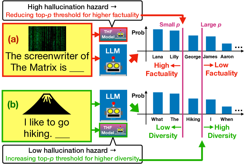
Figure 1: (a) For the factual question, only a few next tokens are correct but the target LLM assigns high probabilities to many tokens, so our THF model predicts the next token from the LLM is likely to be incorrect if using a large $p$ threshold. (b) For the beginning of a sentence, many tokens could be used, so our THF model predicts that sampling from more tokens increases the diversity without hurting the factuality.

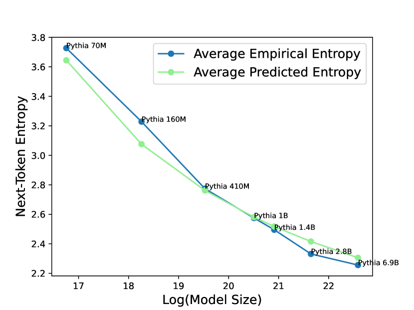
Figure 2: The entropies of the Pythia’s distributions versus the model size in a logarithmic scale. The entropies are averaged across all tokens in a Wikipedia subset. The blue entropy decay curve plots actual entropies from Pythia LMs; the green curve is the entropies predicted by our THF model.

Hallucination is a major problem that limits the applications of LLMs (large language models), especially in open-ended generation tasks [62, 26, 50, 48]. Recent studies show that a LLM often “knows” if it is hallucinating. The findings suggest that the decoding methods of LLMs are major sources of the hallucination.

Sampling is one of the most widely used decoding strategies in LLM due to its simplicity, efficiency, and high generation diversity [25, 24, 37]. Nevertheless, sampling often intensifies an LLM’s hallucination problem. Figure 1 (a) illustrates a simple example. When an LLM is uncertain about who is the screenwriter of a movie, the next-token distribution usually has a high entropy, where some incorrect answers receive high probabilities. Recent studies show that hallucination often happens as the result of such high-entropy distribution and/or the lower probabilities of the sampled tokens [53, 35, 34, 44, 54].

Nucleus (top-$p$) sampling [25] is one of the representative methods proposed to alleviate the issue. By decreasing the constant global $p$ threshold, we can trade the generation diversity for higher factuality [17, 27, 2]. For example, Figure 1 shows that a lower $p$ threshold could reduce the chance of sampling the incorrect writer names in (a), but it would also eliminate the legitimate starts of the possible next sentences in (b). This tradeoff limits nucleus sampling’s ability to generate both high diversity and high factuality outputs. Some existing methods such as typical [37] and eta [24] sampling are proposed to adjust the threshold by characterizing the token-wise distributions of LLM. However, this distribution alone is often not enough to detect the hallucination. For example, both distributions in Figure 1 are similar but the high entropy of (a) arises due to the LLM’s own limitation while that of (b) arises due to the task “inherent uncertainty”.

In this paper, we tackle this problem from a brand-new angle: estimating inherent uncertainty by extrapolating the entropy of LLMs with different sizes. We empirically observe that the entropy of a larger LM’s distribution tends to be smaller as shown in Figure 2. As LLM’s model size becomes larger, the entropy of its distribution should be closer to the inherent uncertainty. As a result, we can extrapolate the entropy decay curve to estimate the asymptotic entropy from an imaginary LLM with an infinite size, which approximates the inherent uncertainty. For example, for the questions discussed in Figure 3 (a), the LLM tends to be more certain about the answer as the size of LLM increases, so we can expect the asymptotic entropy to be low. In contrast, the entropies from different model sizes for the example in Figure 3 (b) should be similar, so we can infer that the next token distribution should have a high asymptotic entropy.

Based on this insight, we propose a tiny unsupervised method to predict the hazard of generating a nonfactual next token, called THF (Token-level Hallucination Forecasting) model. As shown in Figure 3, we parameterize the decay curves of next-token entropies for LLMs and use the THF model to predict the curve parameters. Next, the THF model estimates the LLM’s hallucination hazard by computing the difference between the asymptotic entropy and the LLM’s entropy, which we call the residual entropy (RE). If the LLM is much more uncertain than it should be (i.e., the LLM’s entropy is much larger than the asymptotic entropy), the THF model would forecast a high RE and hence a high hallucination hazard.

Relying on the residual entropy predicted by our THF model, we propose a novel context-dependent decoding method for open-ended text generation, which we call ‘REAL (Residual Entropy from Asymptotic Line) sampling’. REAL sampling adjusts the $p$ threshold in the top-$p$ (nucleus) sampling based on the forecasted hallucination hazard. For example, in Figure 1 (a), the THF model learns that a movie usually does not have many credited screenwriters but the LLM’s distribution entropy is high, so REAL sampling should use a lower threshold to mitigate the hallucination. On the other hand, in Figure 1 (b), THF model learns that the given prompt can be completed in many different ways, so REAL sampling should increase the threshold to boost the generation diversity.

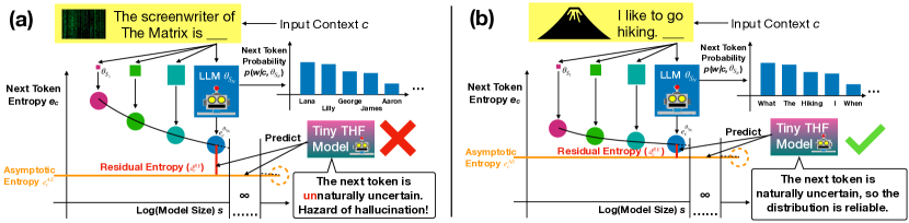
Figure 3: Given the input context, the LLMs with different sizes generate the next-token distributions. By extrapolating the curve using a tiny THF model, we estimate the asymptotic entropy, the entropy from an imaginary LLM with an infinite size (i.e., the inherent uncertainty of the next token), and compute the residual entropy as a measurement of the hallucination hazard. (a) The LLM’s entropy is much higher than the asymptotic entropy. This implies that the LLM is more uncertain than it should be and thus likely to hallucinate next. (b) LLM’s high entropy is fine because the next token is inherently uncertain.

To the best of our knowledge, REAL sampling is the first sampling method that is tightly bounded by the ideal threshold that separates all the factual and nonfactual next tokens without making assumptions on the distribution of the nonfactual next tokens. Besides enjoying the theory guarantee, REAL sampling achieves large and robust empirical improvements in various tasks. In our main experiment, we follow the evaluation protocol in FactualityPrompts [27] and find that sentences generated by Pythia 6.9B LLM [6] with our REAL sampling contains less hallucination and less duplicated n-grams in both in-domain and out-of-domain settings. Our human evaluation indicates that REAL sampling not only improves the factuality but also informativeness, fluency, and overall quality. We further evaluate the generality of the THF model and show improved performance on several hallucination detection tasks. We plan to publicly release our code.

Overall, our main contributions include

• We propose REAL sampling, a context-dependent sampling method that relies on a THF model to predict the asymptotic entropy of an infinitely large LLM to help decide the sampling threshold.

• We theoretically prove that the threshold from our REAL sampling is upperbounded by the ideal value if the top predicted tokens are ideal and the residual entropy is estimated accurately.

• We demonstrate that the tradeoffs between factuality and diversity exist in the 9 state-of-the-art unsupervised sampling methods such as typical sampling [37] and our REAL sampling can consistently boost their factuality given the same diversity, and vice versa. Furthermore, we conduct comprehensive analyses on the THF model and REAL sampling, including evaluating our design choices and their generality using hallucination detection tasks.

2 Preliminary and Motivation

Given a context $c$ and a next token candidate $w$ in a vocabulary $V$, a LLM ($\theta$) outputs the next token probability $p(w|c,\theta)$. Assuming $w^{c}_{i}$ is the $i$th token with the highest probability given the context $c$, top-$p$ (nucleus) sampling first determines the number of tokens $J$ by

$$J=\max_{I}(\{I|\sum_{i=1}^{I}p(w^{c}_{i}|c,\theta)\leq t^{p}\}).$$ (1)

Then, it sets the probabilities from $w_{J+1}$ to $w_{|V|}$ to 0 and re-normalizes the distribution of the top $J$ tokens. In top-$p$ sampling, $t^{p}$ is a fixed global hyperparameter.

As illustrated in Figure 1, lower $t^{p}$ would lead to a better factuality but worse diversity. In practice, many users would like to select from diverse responses. Furthermore, diverse and factual responses could also improve LLM’s performance in reasoning tasks [31, 56, 4, 57, 40]. If we can estimate the hallucination possibility of the next token, we can have a better context-dependent $t^{p}$.

It is notoriously challenging to estimate the hallucination likelihood of each token in general open-ended text generation tasks. One common strategy is to annotate if each generated token is factual and learn a classifier through supervised learning [63]. However, this approach has several drawbacks. First, human annotators often need to take a very long time to check if the generated text is factual, especially in an open-ended generation task, and provide token-level annotation. Second, due to the expense of getting the labels, the classifier is often trained using a few domain-specific examples that are generated by a specific LLM. Therefore, the classifier might not generalize well in other domains, other languages, or other LLMs. This motivates us to develop an unsupervised hallucination forecasting model that only needs the LLMs with different sizes. Then, we can apply our method to any domain, any language, and any LLM without the expensive human annotations.

3 Method

As the LLMs get larger, their performances increase at the cost of higher inference expense, so an institute often trains LLMs (e.g., GPT-4 family [41]) with different sizes using the same training data to let the users balance the cost and quality. We denote the parameters of a LLM family as $\{\theta_{s_{1}},\theta_{s_{2}},...\theta_{s_{N}}\}$, where $s_{n}$ is the size of $n$th model in a logarithmic scale. In this paper, we focus on improving the generation of the largest LLM ($\theta_{s_{N}}$) in its family that can fit into our GPU memory.

In this section, we leverage the LLM family to train a THF model, which aims at predicting the entropy of the ideal (ground-truth) distribution without actually knowing the ideal distribution. In Section 3.1, we first parameterize the entropy decay curve of each next token prediction to predict asymptotic entropy (AE). In Section 3.2, we introduce the architecture of the THF model and how it learns to predict the residual entropy (RE). Finally, we describe REAL sampling, our context-dependent token truncation method based on the THF model in Section 3.3.

3.1 Parameterization and Extrapolation of the Entropy Decay Curve

As we see in Figure 3, the asymptotic entropy (AE) $e_{c}^{AE}$ is the entropy of the next-token distribution from an infinitely-large LLM ($\lim_{s\to\infty}\theta_{s}$). Formally, we define $e_{c}^{AE}$ as

$$\lim_{s\to\infty}e_{c}^{\theta_{s}}=\lim_{s\to\infty}\sum_{w}p(w|c,\theta_{s})\log(p(w|c,\theta_{s})).$$ (2)

To simplify our discussion, we assume an ideal distribution exists and the LLM’s output approaches the ideal distribution as its size increases, so AE measures the next-token inherent uncertainty.

We cannot get the ideal distribution ($\lim_{s\to\infty}p(w|c,\theta_{s})$) when training the LM to predict the next token, which is a crucial challenge of text generation [60]. Consequently, we cannot compute $e_{c}^{AE}$ using Equation 2. Nevertheless, we can use the LLM family to get the pairs of the LLM size and its corresponding entropy $(s_{i},e_{c}^{\theta_{s_{i}}})$ given each context $c$. Then, we can model the entropy decay by formulating it as an one-dimensional regression problem and estimate $e_{c}^{AE}$ by extrapolation.

We propose to parameterize the entropy decay trend using a fractional polynomial [10]:

$$e_{c}(s)=z_{c}+b_{c}(\frac{a_{c,0.5}}{x_{c}(s)^{0.5}}+\sum_{k=1}^{K}\frac{a_{c,k}}{x_{c}(s)^{k}}),$$ (3)

where $s$ is the model size in a logarithmic scale, $x_{c}(s)=\max(1,q_{c}(s-g_{c}))$ is a normalized model size, $e_{c}(s)$ is our entropy prediction, and $a_{c,0.5},a_{c,k},b_{c},q_{c},g_{c}$, and $z_{c}$ are the parameters of the curve. All the parameters are non-negative to ensure the non-increasing property of $e_{c}(s)$. Since $\lim_{s\to\infty}e_{c}(s)=z_{c}$, we can estimate $e_{c}^{AE}$ using $z_{c}$.

Given a context $c$, one approach is to estimate all the $K+5$ parameters by fitting the $(s_{i},e_{c}^{\theta_{s_{i}}})$ on the fly. However, this approach has several problems. First, it is time-consuming to run all the LLMs in the family and fit the curve. Second, we often cannot get many $(s_{i},e_{c}^{\theta_{s_{i}}})$ pairs and the entropy signal of LLMs could be noisy, so the parameter estimation is unstable especially if we want to use a large degree of fractional polynomial $K$. To address the problems, we propose to use a tiny LM to predict the parameters in the next subsection.

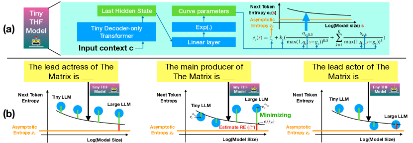
Figure 4: The architecture and the training of the THF model. We use the THF model to predict the parameters of the entropy decay curves and we train the THF model by minimizing the distances between the predicted entropy curves and the empirical entropies from the LLM family.

3.2 Residual Entropy Prediction using the THF Model

The proposed THF (Token-level Hallucination Forecasting) model takes the input context and outputs the parameters of the entropy decay curve. As illustrated in Figure 4 (a), the THF model projects the last hidden state of a pretrained tiny LM decoder to a vector with $K+5$ variables, which are passed through an exponential layer to ensure the positivity of the output parameter predictions.

We train the THF model by minimizing the square root of the mean square error between the predicted entropy and the actual entropy from LLMs. Specifically, our loss could be written as

$$L=\sqrt{\frac{1}{|B|N}\sum_{c\in B}\sum_{i=1}^{N}(e_{c}^{\theta_{s_{i}}}-e_{c}(s_{i}))^{2}},$$ (4)

where $B$ is a training batch.

The entropy signal could be noisy even though all the LLMs are trained on the same corpus. For example, Figure 4 (b), LLM’s entropy of similar contexts are very different, and LLMs with a larger size sometimes have a larger empirical entropy.

Using a tiny model to predict the entropy decay can not only reduce the inference time but also stabilize the parameter estimation. As a model gets smaller, it cannot memorize the small differences between similar input contexts [5], so its predictions tend to be similar given the similar input. For example, when the tiny model receives three similar input contexts in Figure 4 (b), if its hidden states and output parameters for the entropy decay curves are all identical, the gradient descent would encourage the predicted curves to be close to all the empirical entropy measurements of similar context inputs, which effectively increases the number of $(s_{i},e_{c}^{\theta_{s_{i}}})$ pairs and reduces the influence of the noise in the entropy measurements.

As shown in Figure 3, we use the THF model to predict residual entropy (RE) during inference as a measurement of the hallucination hazard:

$$d_{c}^{RE}=e_{c}^{\theta_{s_{N}}}-e_{c}^{AE}\approx\hat{d}_{c}^{RE}=e_{c}(s_{N})-z_{c}.$$ (5)

Notice that although the entropy of LLMs, $e_{c}^{\theta_{s_{N}}}$, is measurable during the inference, we use the predicted entropy $e_{c}(s_{N})$ to estimate the residual entropy $\hat{d}_{c}^{RE}$. This reduces the possible inconsistency between the LLM and the THF model and allows us to estimate the RE without actually running the LLM, which makes our method efficient in hallucination detection applications.

It is worth mentioning that we cannot expect a tiny model to very accurately estimate the inherent uncertainty at every position, which requires the knowledge that even the generation LLM cannot memorize (e.g., how many screenwriters every movie has). Nevertheless, the tiny THF model could still learn that the entropy should be higher at the beginning of a clause but lower if the next token should be something very specific such as an entity. In our experiment, we found that such a rough estimation is sufficient to improve the state-of-the-art decoding methods.

3.3 REAL Sampling

We convert the residual entropy (RE) to the threshold between 0 and 1 for the cumulative probability in Equation 1 using

$$\hat{t}_{c}^{p}=\exp(\frac{-\hat{d}_{c}^{RE}}{T})=\exp(\frac{-\left(e_{c}(s_{N})-z_{c}\right)}{T}),$$ (6)

where $T$ is our temperature hyperparameter used to control the tradeoff between factuality and diversity. When the $T$ is high, the $\hat{t}_{c}^{p}$ would be closer to $1$, so the generation diversity increases at the cost of the lower factuality.

Let’s assume the top tokens from the LLM are factual and its top token distribution is correct (i.e., the same as the distribution of an infinitely large LLM after normalization). Then, there is an ideal threshold $g^{p}_{c}$ for the LLM, which sums the probabilities of all the top factual tokens (e.g., the lower $p$ in Figure 1 (a)), and we can derive an elegant relation between the ideal threshold and the threshold of REAL sampling from an ideal THF model.

Theorem 3.1.

If the residual entropy is estimated accurately (i.e., $\hat{d}_{c}^{RE}=d_{c}^{RE}$), and there is an ideal threshold $g_{c}^{p}$ such that the distribution of the top tokens above the threshold is ideal, then

$$t_{c}^{p}=\exp(\frac{-d_{c}^{RE}}{T})\leq(g_{c}^{p})^{\frac{1}{T}}.$$ (7)

Please see our proof in Appendix B. That is, when the ideal threshold exists and our RE is accurate, our threshold $t_{c}^{p}$ is not larger than the ideal threshold raised to power $\frac{1}{T}$.

4 Experiments

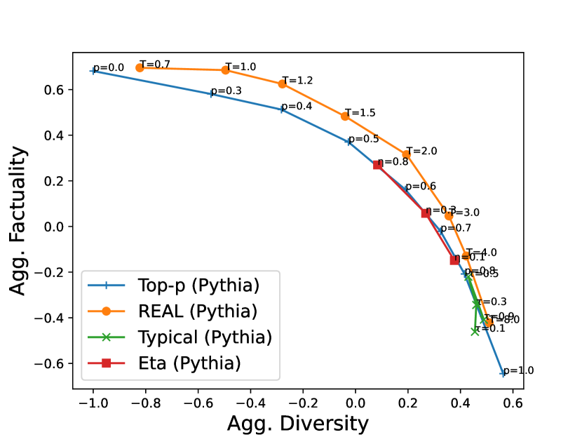
(a) REAL vs Thresholding Methods

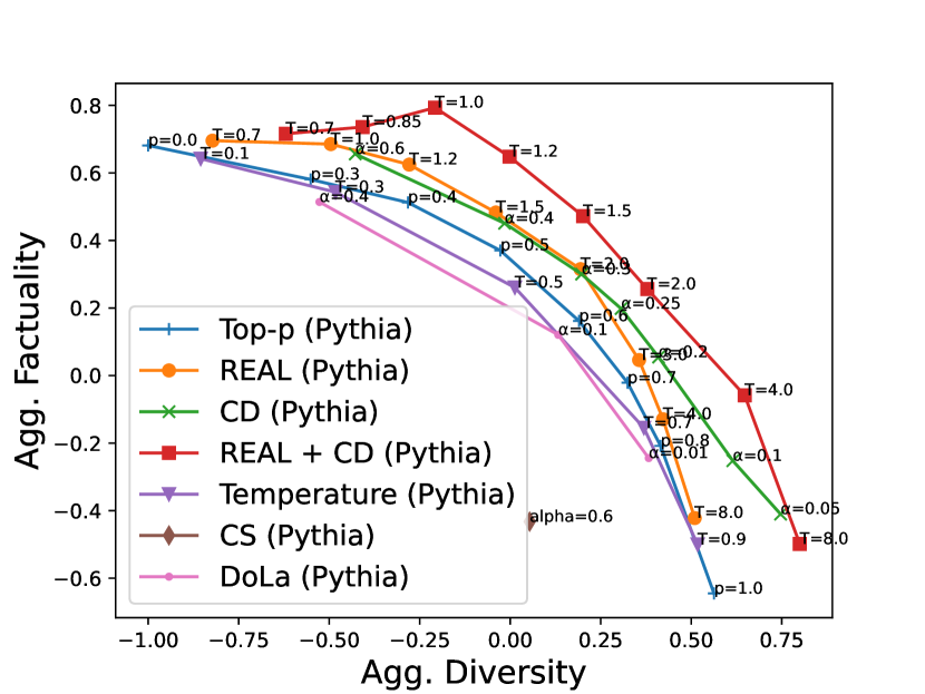
(b) REAL vs Distribution Modifications

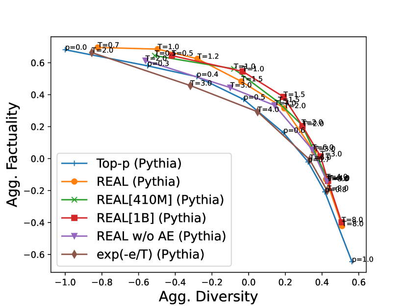
(c) Comparison of the THF model sizes and ablation on our dynamic thresholding formula

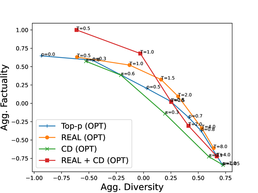
(d) Using OPT-6.7b as the generation LLM and the THF model trained on Pythia.

Figure 5: Open-ended text generation performance comparison between REAL sampling and state-of-the-art unsupervised thresholding methods, including top-$p$ [25], eta [24], and typical [37] sampling. The factuality and diversity are evaluated using the FactualityPrompts benchmark from Lee et al. [27]. We also conduct an ablation study and compare REAL sampling with the distribution modification methods including temperature sampling [19], contrastive search [47] (CS), contrastive decoding (CD) [30] and DoLa [13]. See more comparisons at Figure 9, Figure 11, and Figure 13.

We evaluate our REAL sampling using the FactualityPrompts benchmark [27] and using human evaluation in this section. In Appendix C and Appendix D, we evaluate our methods in hallucination detection and entropy curve regression tasks, respectively.

We use the de-duplicated variant of Pythia LLM series [6] to train our THF model. By default, we use Pythia 6.9B as our LLM generation model ($\theta_{s_{N}}$) and the THF model is based on the transformer from Pythia 70M.

4.1 Retrieved-based Evaluation using FactualityPrompts

Setup: Lee et al. [27] propose an evaluation benchmark, FactualityPrompts, for open-ended text generation that first lets different LLMs generate continuations of each prompt sentence and retrieves the relevant Wikipedia pages [23] to evaluate the factuality of the generation.

FactualityPrompts provides 8k factual sentences and 8k nonfactual sentences from FEVER [49] as the prompts. We use the first 1k (non)factual prompts as our validation set to select the THF models and the rest 7k prompts as our test set. For each decoding method, the LLM generates 4 continuations for each prompt.

Metrics: FactualityPrompts uses Entail_R and NE_ER to evaluate the factuality. Entail_R is the ratio of the generated sentences entailed by the sentences in the relevant Wikipedia pages, while NE_ER is the ratio of the entities that are not in the pages. Both metrics are shown to have high correlations ($\sim$0.8) with the hallucination labels from an expert [27]. Lee et al. [27] use distinct n-grams (Dist-n) [28] to measure the diversity across generations and repetition ratio (Rep) [25] to measure the diversity within a generation. A good method should get high Entail_R and Dist-n, but low NE_ER and Rep.

To compare the performances of methods in one figure, we first normalize all metrics from a generation LLM using max-min normalization and average the scores from both factual prompts and nonfactual prompts as Entail_Rn, NE_ERn, Dist-2_n, and Rep_n. Next, we define the aggregated metrics

$$\text{Agg. Factuality}=\text{Entail}_{Rn}-\text{NE}_{ERn},\;\;\;\;\text{and}\;\;\;\;\text{Agg. Diversity}=\text{Dist-2}_{n}-\text{Rep}_{n}.$$ (8)

The scores of the original 4 metrics will be reported in Section E.3.

Methods: We compare multiple variants of our (ablated) methods described in detail below, with several state-of-the-art decoding methods such as top-$p$ [25], eta [24], typical [37] sampling, temperature sampling [19], contrastive search [47] (CS), contrastive decoding (CD) [30] and DoLa [13].

• REAL (Pythia): REAL sampling using 70M THF model.

• REAL + CD (Pythia): Combining our methods with contrastive decoding (CD) [30]. We first truncate the tokens using the threshold $\hat{t}_{c}^{p}$ in REAL sampling and apply the contrastive decoding (i.e., computing the probabilities of the top tokens using the logit differences between $\theta_{s_{N}}$ and $\theta_{s_{1}}$).

• REAL[410M] or REAL[1B] (Pythia): REAL sampling using 410M or 1B THF model.

• REAL w/o AE (Pythia): Our method after removing the asymptotic entropy (AE) estimation as $\hat{t}_{c}^{p}=\exp(\frac{-e_{c}(s_{N})}{T})$.

• exp(-e/T) (Pythia): Instead of using THF model to predict the entropy of LLM, we estimate the entropy from LLM and set $\hat{t}_{c}^{p}=\exp(\frac{-e_{c}^{\theta_{s_{N}}}}{T})$. The method simply reduces the $p$ threshold whenever encountering a flat distribution (e.g., distributions in both (a) and (b) of Figure 1).

• * (OPT): In the methods, we replace the Pythia 6.9B with OPT-6.7b [59] as the generation LLM, respectively. Notice that the THF model is still trained using the Pythia family.

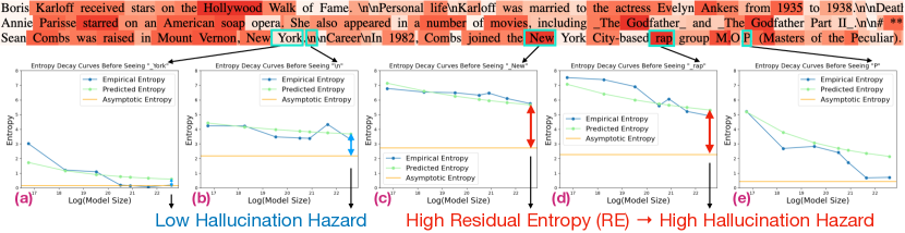
Figure 6: The visualization of the estimated residual entropy ($\hat{d}_{c}^{RE}$) and entropy decay curves. The top three lines come from the first three testing factual prompts in FactualityPrompts and continuations generated by Pythia 6.9B. A darker red highlights a larger hallucination hazard ($\hat{d}_{c}^{RE}$) forecasted by our THF model based on the context before the position, and thus it leads to a smaller $p$ threshold in REAL sampling. The bottom figures (a)-(e) visualize the empirical entropy decay curves from five tokens in the third example, along with the corresponding curves predicted by our THF model and asymptotic entropies.

Results: In Figure 5(a), REAL sampling consistently outperforms top-$p$, eta, and typical sampling across the whole spectrum. Overall, we often improve the factuality more when the temperature $T$ is low (i.e., diversity is relatively low) probably because lower $T$ emphasizes the effect of $\hat{d}_{c}^{RE}$ in Equation 6. Notice that some diversities actually come from hallucination, so it is hard to increase the diversity and the factuality at the same time, especially by only adjusting the truncation threshold without changing the distribution of LLM like our methods. In Figure 5(b), REAL + CD is prominently better than using contrastive decoding CD alone, which shows that REAL sampling is complimentary with other distribution modification methods.

In Figure 5(c), the worse performance of REAL w/o AE (especially with low diversity) verifies the effectiveness of predicting asymptotic entropy (AE). The 70M THF model (REAL) performs similarly compared to the larger THF models (REAL (410M) and REAL (1B)), and using the LLM entropy predicted by THF model (REAL w/o AE) is much better than using the empirical LLM entropy (exp(-e/T)). These two results in our ablation study suggest that a tiny model indeed stabilizes the entropy decay curve prediction (see Section D.1 and Appendix F for more details).

To evaluate our generalization capability, we use the THF model trained on the Pythia family to improve OPT. Figure 5(d) indicates that REAL sampling can still improve the factuality, and the improvement is especially prominent if CD is used. To explain the strong generalization ability across the serious misalignment between the training and testing objectives, we visualize the residual entropy (RE) from our THF model in Figure 6. We observe that the residual entropy tends to be larger at the positions where the LLMs generally are more likely to hallucinate. For example, in (c), the THF model forecasts a high hallucination hazard for New, which is the first token in an entity name. Nevertheless, we also observe that the THF model cannot always predict LLM’s entropy accurately due to its small size, and (e) is an example. Finally, Section E.2 shows that REAL sampling can also improve OpenLLaMA2-7b [21], factual sampling [27], and top-$k$ [18].

Table 1: Human evaluation for the open-ended generation. We highlight the better number between win and loss. $\dagger$ the win is significantly more than lose under Fisher’s exact test [20] with $p=0.5$.

Model Comparision	Overall			Factuality			Informativeness			Fluency
	win	tie	loss	win	tie	loss	win	tie	loss	win	tie	loss
REAL   vs   Top-$p$	29.5$\dagger$	53.5	17	26	53.5	20.5	26	51	23	24.5$\dagger$	58.5	17
REAL+CD   vs   CD	27$\dagger$	53	20	23.5	53.5	23	26.5	52	21.5	19.5	64.5	16
CD   vs   Top-$p$	34.5$\dagger$	46	19.5	31$\dagger$	49.5	19.5	33.5$\dagger$	41.5	25	25.5	53.5	21
REAL+CD   vs   Top-$p$	38$\dagger$	44	18	35.5$\dagger$	43	21.5	30.5$\dagger$	45.5	24	27$\dagger$	54.5	18.5

4.2 Human Evaluation

To verify that our methods are still better from the humans’ perspective, we ask the workers from Amazon Mechanical Turk (MTurk) to evaluate the factuality and the quality of the generated continuations using the Internet. Given 100 factual prompts in FactualityPrompts, we generate the next sentences using Top-$p$ ($p=0.6$), REAL ($T=2.0$), CD ($\alpha=0.3$), and REAL + CD ($T=1.5$) because the methods have similar diversity. In each task, the workers are asked to judge their factuality, fluency, informativeness, and overall quality. In the meanwhile, each worker needs to provide the URL(s), the statement(s) in the URL(s), and/or reason(s) that can justify their factuality annotations. Given a metric and a decoding method in a task, the worker provides a $1$ to $5$ score and we compare the scores to get the pairwise comparison results. Every task is answered by 2 workers.

Results: In Table 1, our methods constantly outperform the corresponding baselines (i.e., REAL wins Top-$p$ more and REAL + CD wins CD more) and the improvement of REAL + CD vs Top-$p$ is larger than CD vs Top-$p$. The factuality evaluation results verify the effectiveness of the retrieved-based evaluation. Furthermore, our methods also achieve better informativeness and fluency. Consequently, we get the largest improvement in the overall metric.

5 Related Work

Due to the importance of LLM’s hallucination problems, various mitigation approaches are proposed. For a comprehensive discussion, please see the recent surveys from Huang et al. [26], Tonmoy et al. [50]. Nevertheless, as far as we know, no existing sampling methods that can improve both factuality and diversity in open-ended text generation without annotations or domain-specific heuristics/assumptions.

Some methods can improve the factuality by relying on some domain-specific assumptions. For example, Lee et al. [27] assume the hallucination is more likely to appear at the latter part of a sentence. Burns et al. [7] assume there is a set of statements that are either true or false. Several studies [53, 35, 9, 45, 11] assume that the generated text should be relevant to a source document. These methods might not be applicable to other domains (e.g., other languages or open-ended text generation tasks) and could (potentially) be combined with our method to achieve better performance in the specific domain (e.g., see Figure 13(b) and Appendix I).

In terms of high-level methodology, our method is related to some recent extrapolation-based methods in other applications. For example, Das et al. [15] use a linear regressor to extrapolate the distribution of a deeper LM, Lu et al. [33] extrapolate the probability distribution to get negative examples for text quality assessment, and Zheng et al. [61] extrapolate the weights of a LM after training on more preference data. However, none of them studies the threshold for sampling the next-token distribution.

6 Conclusion

Figure 1 suggests that it is difficult or sometimes even impossible in open-ended text generation tasks to predict the hallucination likelihood of the next token only based on the LLM’s distribution without considering the inherent uncertainty of the task. In this paper, we demonstrate the feasibility of training a tiny model to forecast the hallucination hazard of LLM without supervision and domain-specific heuristics. Based on this finding, we propose REAL sampling along with its theoretical guarantee. Our comprehensive experiments indicate that most existing sampling methods cannot consistently outperform top-$p$ sampling in FactualityPrompts. In contrast, our proposed REAL sampling not only outperforms top-$p$ sampling but also can be combined with other decoding methods (e.g., contrastive decoding) to further reduce hallucination. We also demonstrate a THF model trained on one LLM family could be used to forecast/detect the hallucination from the LLM from another family, which highlight the strong out-of-domain generalization ability of our THF model.

Appendix

Appendix A Overview

In the appendix, we prove Theorem 3.1 in Appendix B, use the residual entropy to detect hallucination in Appendix C, explore different parameterizations of the entropy decay function and different THF model sizes in Appendix D, provide more experiment results in Appendix E, provide more explanation to the empirical observations in Appendix F, test REAL sampling for a creative writing task in Appendix G, provide our impact statements in Appendix H, describe our limitation and future work in Appendix I, discuss why the entropy decreases as the model size increases in Appendix J, report more implementation details of our method in Appendix K, report more experimental details in Appendix L.

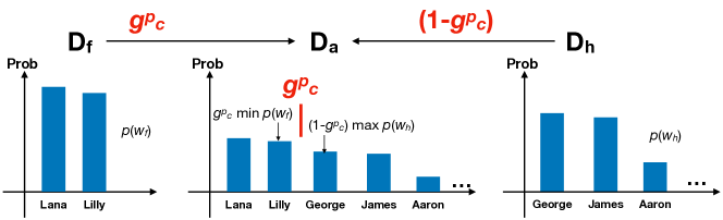
Figure 7: Illustration of the notations used in Appendix B. All the next tokens are sorted based on its probabilities.

Appendix B Proof of Theorem 3.1

Proof.

To simplify our notations, we write the conditional probability $p(w|c)$ as $p(w)$ in the following derivation and Figure 7 since every probability is conditioned on $c$.

In Figure 7, we illustrate our notations. One condition of Theorem 3.1 is that the top token distribution is ideal, so we can decompose the next-token distribution $D_{a}$ into factual/ideal distribution $D_{f}$ (i.e., the distribution from an infinitely large LLM) and hallucination distribution $D_{h}$ that we want to truncate. We denote the factual token as $w_{f}$ and the hallucinated tokens as $w_{h}$. The ideal $p$ threshold that separates two distributions is $g^{p}_{c}$, so the probabilities of each factual token and hallucinated token in $D_{a}$ are $g^{p}_{c}\cdot p(w_{f})$ and $(1-g^{p}_{c})\cdot p(w_{h})$, respectively. From Figure 7, we can see that

$$g^{p}_{c}\min_{w_{f}}(p(w_{f}))\geq(1-g^{p}_{c})\max_{w_{h}}(p(w_{h})).$$ (9)

The condition of Theorem 3.1 states that $\hat{d}_{c}^{RE}=d_{c}^{RE}$, so we know

$$t_{c}^{p}=\exp(\frac{-d_{c}^{RE}}{T})=\exp(\frac{Ent(D_{f})-Ent(D_{a})}{T}),$$ (10)

where $Ent(D)$ is the entropy of the distribution $D$.

Based on the above two conditions, we can get

$$-T\cdot\log(t_{c}^{p})=Ent(D_{a})-Ent(D_{f})$$

$$=-\sum g^{p}_{c}\cdot p(w_{f})\log(g^{p}_{c}\cdot p(w_{f}))-\sum(1-g^{p}_{c})\cdot p(w_{h})\log((1-g^{p}_{c})\cdot p(w_{h}))-Ent(D_{f})$$

$$=g^{p}_{c}\cdot Ent(D_{f})-g^{p}_{c}\log(g^{p}_{c})+(1-g^{p}_{c})\cdot Ent(D_{h})-(1-g^{p}_{c})\log(1-g^{p}_{c})-Ent(D_{f})$$

$$=-(1-g^{p}_{c})\cdot Ent(D_{f})+(1-g^{p}_{c})\cdot Ent(D_{h})+(1-g^{p}_{c})\log(g^{p}_{c})-(1-g^{p}_{c})\log(1-g^{p}_{c})-\log(g^{p}_{c})$$

$$=(1-g^{p}_{c})\left(Ent(D_{h})-Ent(D_{f})+\log(g^{p}_{c})-\log(1-g^{p}_{c})\right)-\log(g^{p}_{c})$$

$$=(1-g^{p}_{c})\left(-\sum p(w_{h})\log(p(w_{h}))+\sum p(w_{f})\log(p(w_{f}))+\log(\frac{g^{p}_{c}}{1-g^{p}_{c}})\right)-\log(g^{p}_{c})$$

$$\geq(1-g^{p}_{c})\left(-\sum p(w_{h})\log(\max_{w_{h}}p(w_{h}))+\sum p(w_{f})\log(\min_{w_{f}}p(w_{f}))+\log(\frac{\max\limits_{w_{h}}p(w_{h})}{\min\limits_{w_{f}}p(w_{f})})\right)-\log(g^{p}_{c})$$

$$=-\log(g^{p}_{c})$$

Therefore,

$$t_{c}^{p}=\exp(\frac{-d_{c}^{RE}}{T})\leq(g_{c}^{p})^{\frac{1}{T}}.$$ (11)

∎

Table 2: Hallucination detection in open-ended text generation. A random forest classifier predicts the hallucination using the features from Pythia 6.9B LLM, Pythia 70M LM, and THF model. 1 Feature (6.9B per) refers to only using the perplexity of Pythia 6.9B to detect hallucination [39, 54]. The better performances in each section are highlighted.

Dataset $\rightarrow$	Factor						TF ext		HaDes		Avg
Creation Method $\rightarrow$	Revising a Factual Sentence using ChatGPT						Template + Table		BERT Infill
Subset / Size $\rightarrow$	Wiki / 47025		News / 7663		Expert / 355		All / 9830		All / 1000
Feature Subsets $\downarrow$ Metrics $\rightarrow$	1-4 ACC	AUC	1-4 ACC	AUC	1-4 ACC	AUC	ACC	AUC	ACC	AUC
1 Feature ($6.9B\_per$)	0.374	0.315	0.367	0.312	0.347	0.290	0.619	0.691	0.528	0.599	0.444
2 Features ($6.9B\_per$ + $heur\_ent$)	0.424	0.322	0.359	0.313	0.347	0.300	0.624	0.700	0.503	0.581	0.447
2 Features ($6.9B\_per$ + $RE$)	0.393	0.319	0.390	0.303	0.364	0.320	0.635	0.711	0.521	0.580	0.454
6 Freatures (6.9B and 70M)	0.490	0.341	0.432	0.326	0.534	0.356	0.654	0.754	0.578	0.646	0.511
All (6.9B, 70M, $RE$, and $AE$)	0.498	0.341	0.465	0.326	0.619	0.346	0.671	0.769	0.565	0.669	0.527

Appendix C Hallucination Detection for Open-ended Text Generation

Perplexity and entropy are widely used to detect the hallucination [53, 35, 39, 34, 44, 54]. However, high perplexity or entropy could mean multiple correct answers instead of hallucination as in Figure 1 (b), so we test if the residual entropy (RE) and asymptotic entropy (AE) could be useful unsupervised signals for the hallucination detection tasks.

Setup: We test the features using three hallucination detection datasets: Factor [39], extended True-False dataset (TF ext) [3], and HaDes [32]. We train a random forest classifier to combine these unsupervised features from the input context and phrase/sentence.

Metrics: The goal of all three datasets is to classify the text into either factual or nonfactual, so we can use the area under the precision recall curve (AUC) to measure the performances of classifiers. In the Factor dataset, one of the four sentence continuations is factual. Thus, we follow Muhlgay et al. [39] to measure the accuracy of detecting the factual sentence (1-4 ACC). In TF ext and HaDes, we also report the accuracy of the classifiers. To summarize the performance of each method, we report the average of all the scores.

Methods: We consider the following features:

• Perplexity of Pythia 6.9B ($6.9B\_per$),

• Entropy of Pythia 6.9B ($6.9B\_ent$),

• Perplexity of Pythia 70M ($70M\_per$),

• Entropy of Pythia 70M ($70M\_ent$),

• $\sqrt{6.9B\_per\cdot\max(0,70M\_per-6.9B\_per)}$ ($heur\_per$)

• $\sqrt{6.9B\_ent\cdot\max(0,70M\_ent-6.9B\_ent)}$ ($heur\_ent$)

• $\hat{d}_{c}^{RE}$ in Equation 5 ($RE$)

• $z_{c}$ in Equation 3 ($AE$),

where all features are averaged across the tokens in the input phrase/sentence, and $heur\_ent$ is a simple hallucination detection heuristic that approximates $RE$. If the next token is a hallucination, it should have a high LLM entropy and large entropy difference between the LLM and the smallest LM in the family as in Figure 3 (a).

Given a subset of the above features, we conduct an exhaustive feature selection to boost/stabilize the performance and train a random forest classifier with 100 estimators.

Results: In Table 2, 2 Features ($6.9B\_per$ + $RE$) usually outperforms 2 Features ($6.9B\_per$ + $heur\_ent$) and 1 Feature ($6.9B\_per$), which indicates that adding the $RE$ features can improve the widely-used perplexity measurement of LLM [39, 54] and the improvement cannot be achieved by the heuristics that try to leverage the same signal. Similarly, compared to 6 Features (6.9B and 70M), the better performance of All (6.9B, 70M, $RE$, and $AE$) demonstrates that even letting the random forest combine all the features from the Pythia 6.9B and 70M, residual entropy (RE) and asymptotic entropy (AE) from our THF model still provide extra information for hallucination detection.

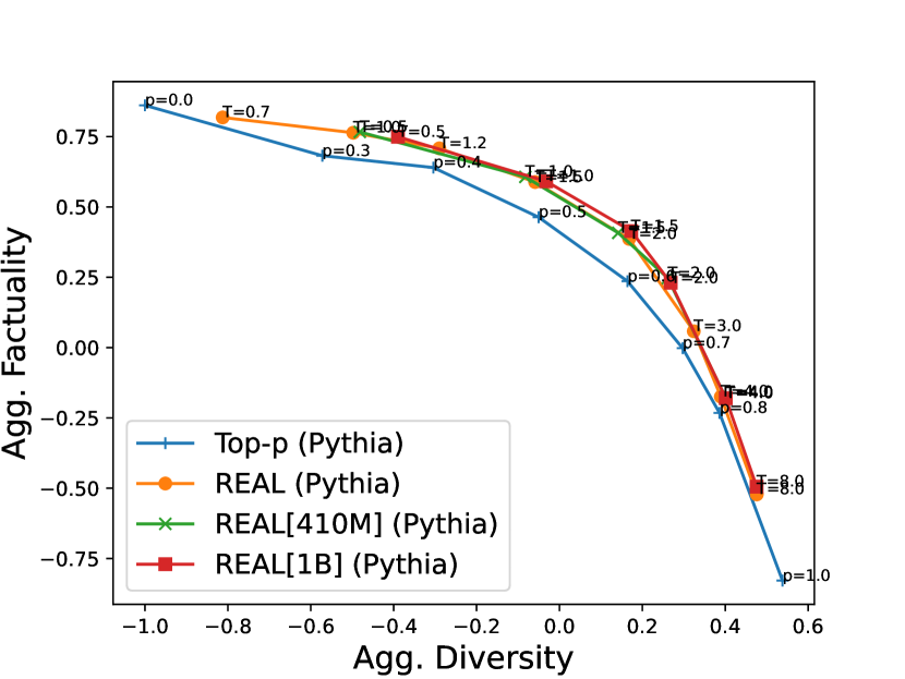
(a) Factual + Nonfactual

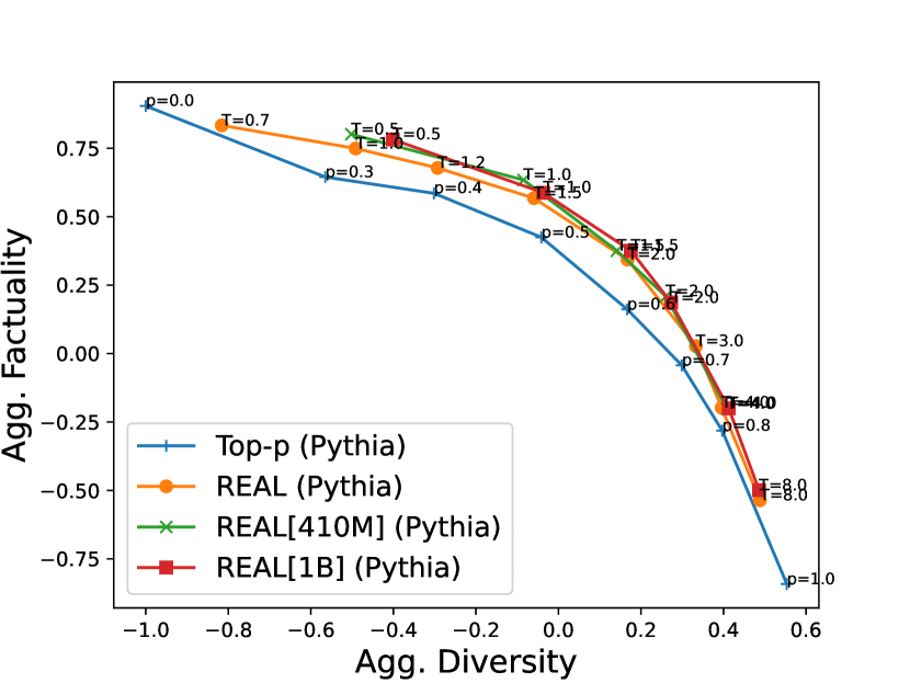
(b) Factual

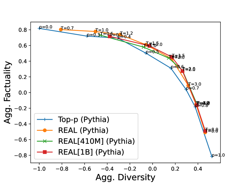
(c) Nonfactual

Figure 8: Comparing different sizes of THF models. REAL means REAL[70M]. We evaluate 3 sentences after the prompt.

Appendix D Analyses of Entropy Decay Modeling

We conduct a serious experiments to examine the influence of different design choices on our THF model, including its model size in Section D.1, its $K$ value (i.e., highest order of fractional polynomial) in Section D.2, and its fractional polynomial parameterization function in Section D.3. We also compare regresion error of predicting the LLM’s entropy using different parameterization functions in Section D.4.

D.1 Choice of the THF Model Size

We find that the performance is not sensitive to the choice of the THF model size. Figure 8(a) shows that the REAL sampling based on different sizes of THF models performs similarly in FactualPrompts. Nevertheless, we find that larger models perform slightly better given factual prompts in Figure 8(b), while the 70M model performs slightly better given nonfactual prompts in Figure 8(c). Since THF is trained only on factual text, the results suggest that a larger model could perform better in an in-domain setting due to its more accurate entropy decay modeling. On the other hand, a smaller THF model is better at handling the noise both in the input context and in the entropy decay curves as illustrated in Figure 4, and hence has a strong out-of-domain generalization capability.

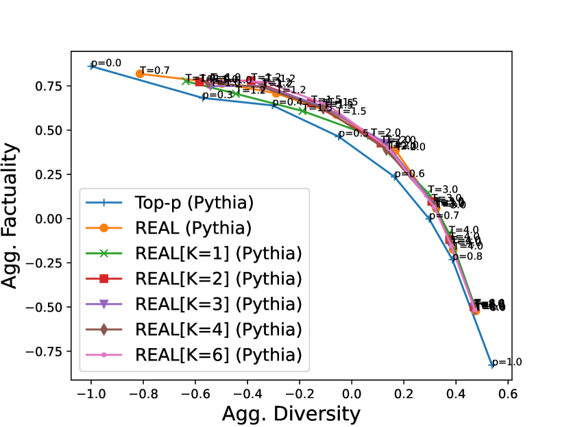
(a) Factual + Nonfactual

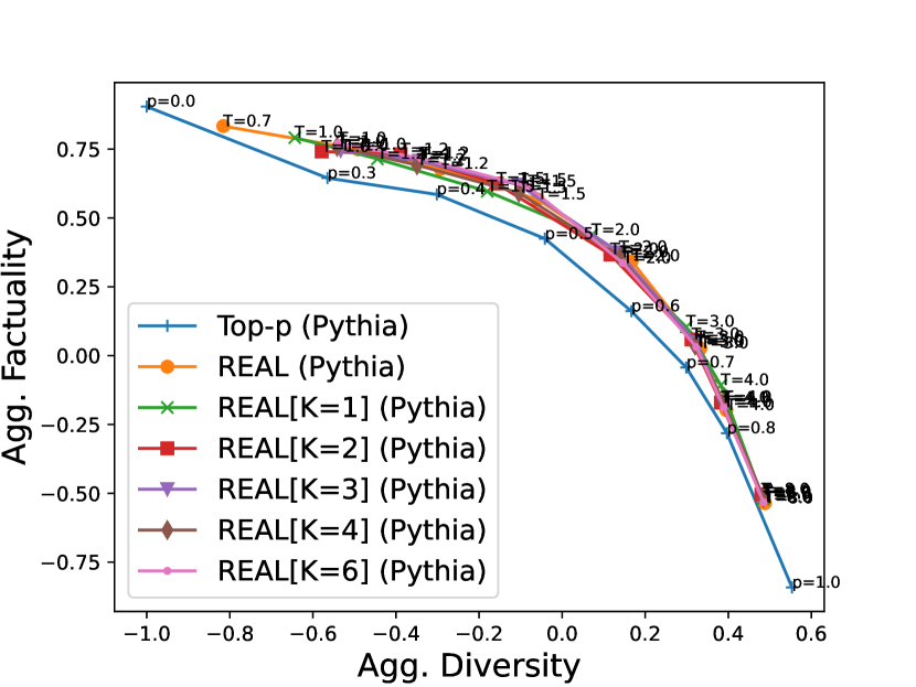
(b) Factual

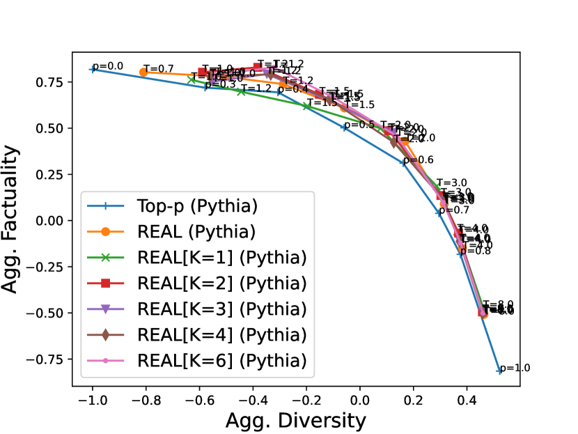
(c) Nonfactual

Figure 9: Comparison of Pythia generation performance in FactualPrompt benchmark given different K (highest degrees of fractional polynomial). REAL means REAL[K=10]. We evaluate 3 sentences after the prompt.

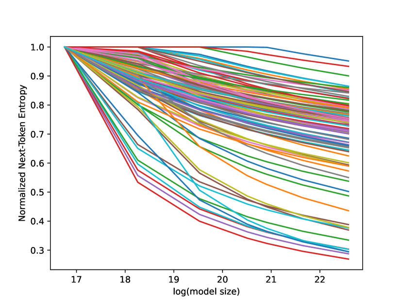
(a) K=1

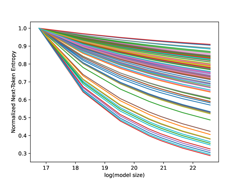
(b) K=2

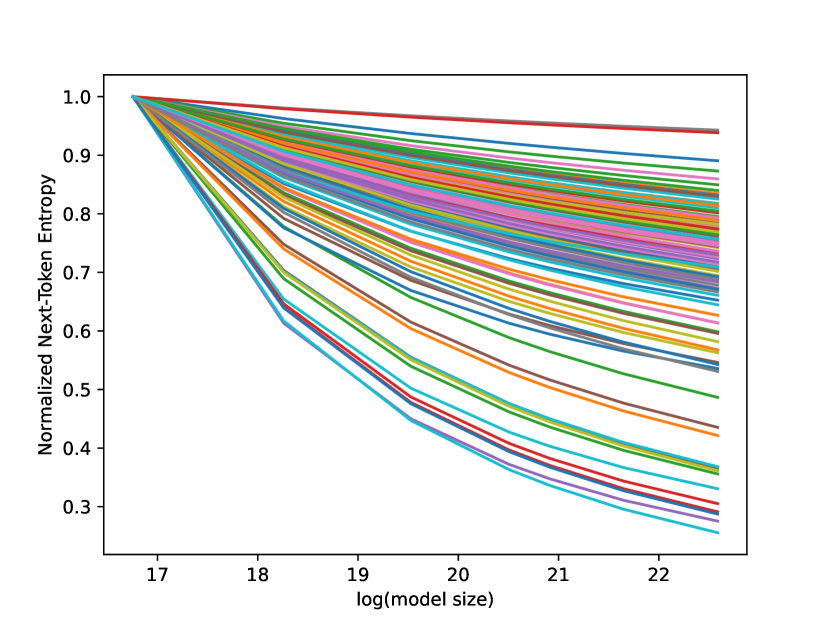
(c) K=10

Figure 10: Normalized entropy decays predicted by the THF models with different $K$ (i.e., highest degree of the fractional polynomial). We normalize the predicted entropies by the predicted entropy of 70M Pythia (to make all the curves start from 1 given the model size of the smallest LM) and plot the curves for the first 100 tokens in our validation set.

D.2 Choice of K

We set the highest order of fractional polynomial ($K$) as $10$ because we find that the performance is not sensitive to the choice of $K$ once $K$ is larger than a number. In Figure 9(a), the performance of REAL sampling stays almost the same when $K>=2$, but the performances of $K=1$ drop significantly.

To explain the observation, we compare the normalized entropy decays of the models with $K=1$, $K=2$, and $K=10$ using the first 100 tokens in our validation set. Figure 10 shows that the curves from $K=2$ and $K=10$ are very similar while the curves from $K=1$ are different. This indicates that increasing the $K$ to $10$ for the THF model does not have a serious overfitting problem because it could learn to assign $0$ weight to the unnecessary terms in fractional polynomials. Nevertheless, similar to the findings in the last section, we observe that a more complex THF model (i.e., a higher $K$ or a larger model size) seems to perform slightly better given factual prompts in Figure 9(b) due to its prediction power but performing slightly worse given nonfactual prompts in Figure 9(c).

Table 3: Comparing LLM’s entropy predictions $e_{c}(s_{N})$ from different THF models using regression metrics. FP means fractional polynomials we used in Equation 3.

	Pearson r	R2	MSE ($\downarrow$)	Mean L1 ($\downarrow$)
Exp	0.843	0.708	0.786	0.64
Logistic	0.842	0.707	0.788	0.641
FP[K=10] (REAL)	0.843	0.71	0.78	0.639
FP[K=6]	0.843	0.71	0.781	0.639
FP[K=4]	0.844	0.712	0.776	0.636
FP[K=3]	0.843	0.709	0.782	0.64
FP[K=2]	0.844	0.711	0.778	0.638
FP[K=1]	0.844	0.711	0.777	0.641

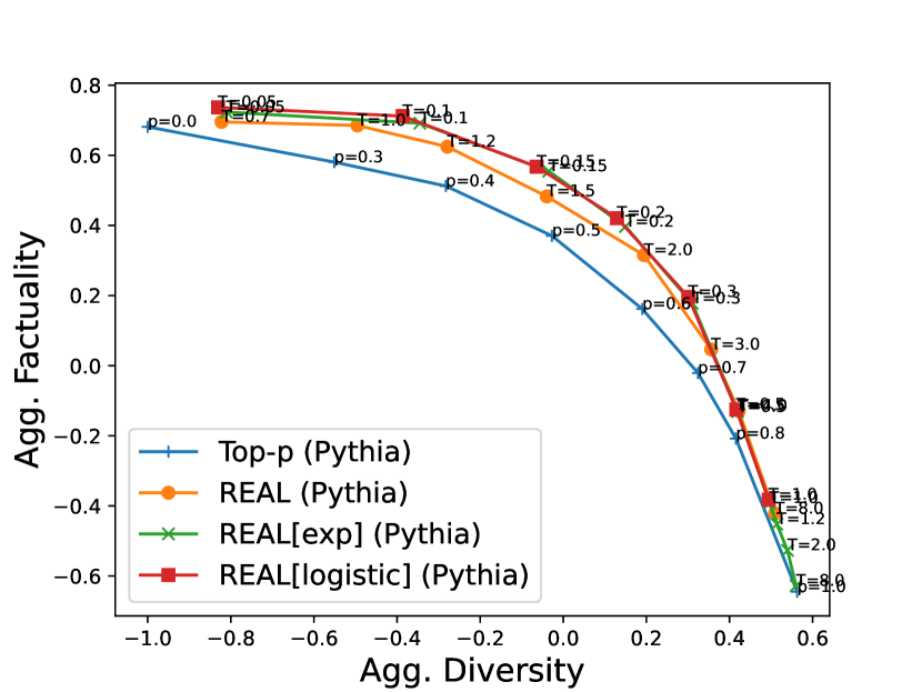
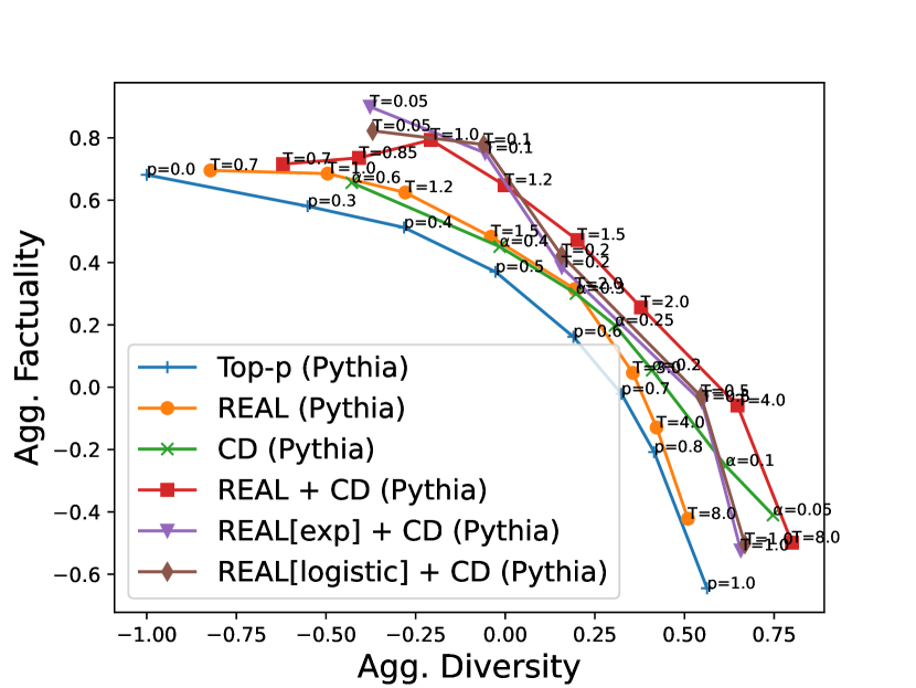
Figure 11: Comparison of Pythia generation performance in FactualPrompt using different functions to model the entropy decay. REAL uses fractional polynomials in Equation 3; REAL[exp] uses exponential decay functions $e_{c}(s)=z_{c}+b_{c}\exp(-\max(0,q_{c}(s-g_{c})))$; REAL[logistic] uses logistic decay function ($e_{c}(s)=z_{c}+\frac{b_{c}}{1+\exp(-\max(0,q_{c}(s-g_{c})))}$).

D.3 Choice of the Entropy Decay Functions

In our experiments, we use fractional polynomials (FPs) to parameterize the entropy decay function in Equation 3. When practitioners deploy the REAL sampling, more non-increasing functions could be tried. We recommend using FPs by default because of its flexibility. Given a new LLM family, we are not sure how fast their entropy decays would be, so it is good to let the THF model learn the weight of each term in the FP. To further justify the choice, we also try an exponential (exp) decay function ($e_{c}(s)=z_{c}+b_{c}\exp(-\max(0,q_{c}(s-g_{c})))$) and a logistic decay function ($e_{c}(s)=z_{c}+\frac{b_{c}}{1+\exp(\max(0,q_{c}(s-g_{c})))}$).

In Figure 11, all the parameterization functions provide significant improvement for Pythia 6.9B LLM and the FP is slightly worse than the other ways. Nevertheless, after being combined with contrastive decoding (CD), the FP performs better for high temperature/diversity while other functions perform better for low temperature/diversity. Figure 14(h) indicates that the exponential and logistic functions have a higher repetition rate after being combined with CD, especially when the temperature/diversity is high. This drawback makes FP’s improvement more consistent across all settings.

D.4 Regression Metrics

The goal of our THF model is to predict the difference between the entropy of generation LLM ($e_{c}^{\theta_{s_{N}}}$) and entropy of the infinitely-large LLM ($e_{c}^{AE}$). Since we cannot access infinitely-large LLM, we validate our prediction of $e_{c}^{\theta_{s_{N}}}$ (i.e., $e_{c}(s_{N})$).

We compare different parameterization functions, including exponential (exp), logistic, and fractional polynomial function, and also different $K$ values using Pearson correlation coefficient (r), mean squared error (MSE), average L1 norm (Mean L1), and coefficient of determination (R2)[16].

Table 3 indicates that all methods perform similarly well. Even though our THF model only has 70M parameters, it can predict the entropy of 6.9G LLM accurately by achieving around $0.84$ Pearson correlation coefficient (r). The fractional polynomials are slightly better than other parameterizations, including exponential and logistic functions and the prediction performance is not sensitive to the maximal degree of our fractional polynomial ($K$).

Appendix E More Results for FactualityPrompts

In this section, we evaluate longer continuations in Section E.1, combine REAL sampling with top-$k$ and factual (F) sampling and test REAL sampling on OpenLLaMA-7b [21] in Section E.2, analyze the scores of every metric provided by FactualityPrompts in Section E.3, report the speed of our implementation in Section E.4, and report additional statistics in our human experiment for content writing in Section E.5.

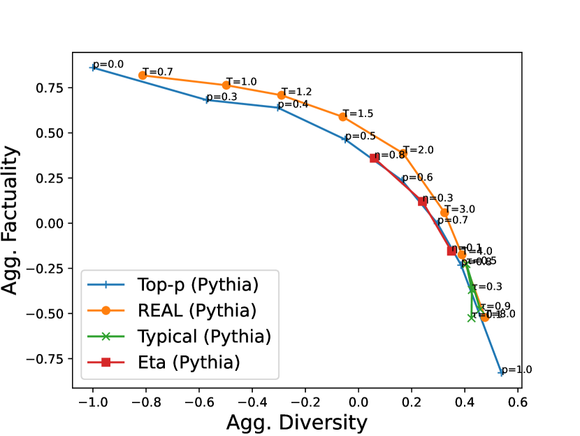
(a) REAL vs Thresholding Methods

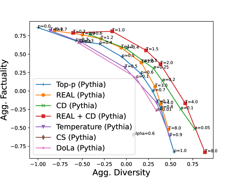
(b) REAL vs Distribution
Modifications

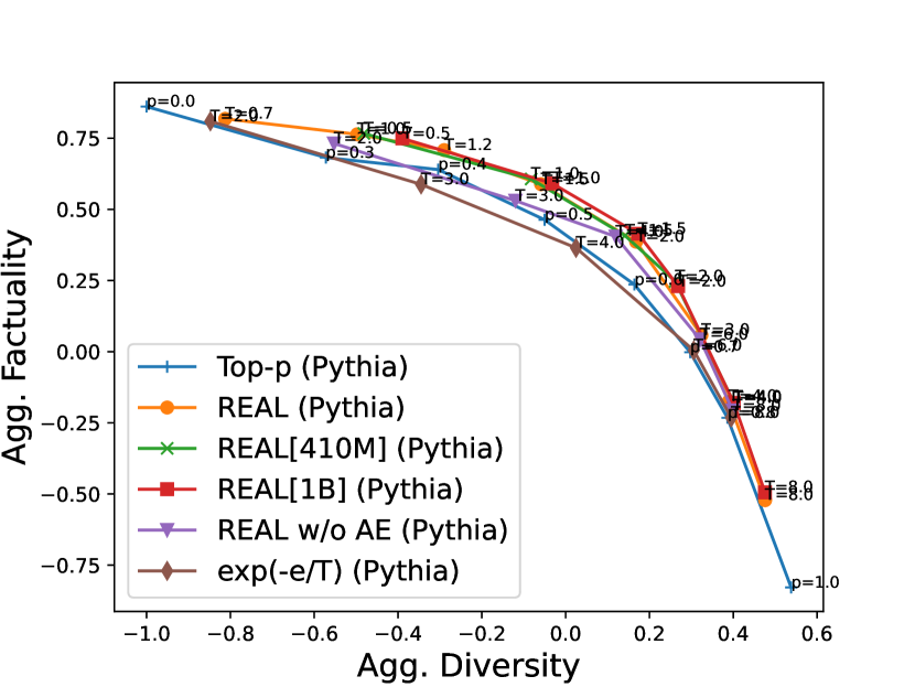
(c) Ablation

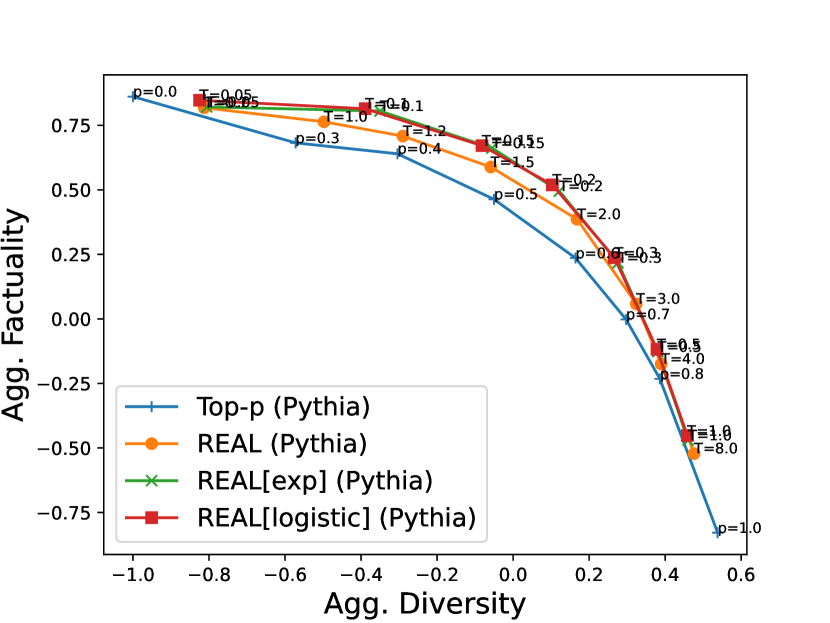
(d) Different Parameterizations

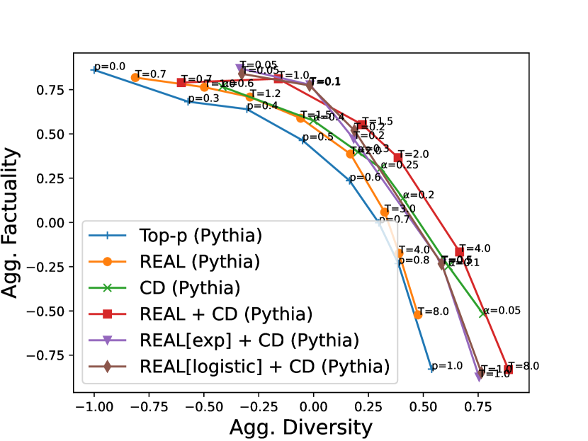
(e) Different Parameterizations

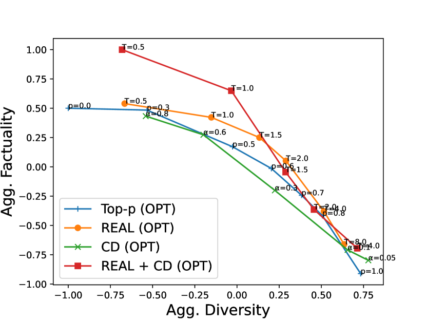
(f) OPT-6.7b

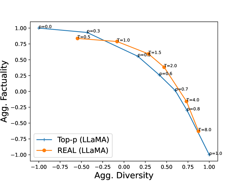
(g) OpenLLaMA-7b

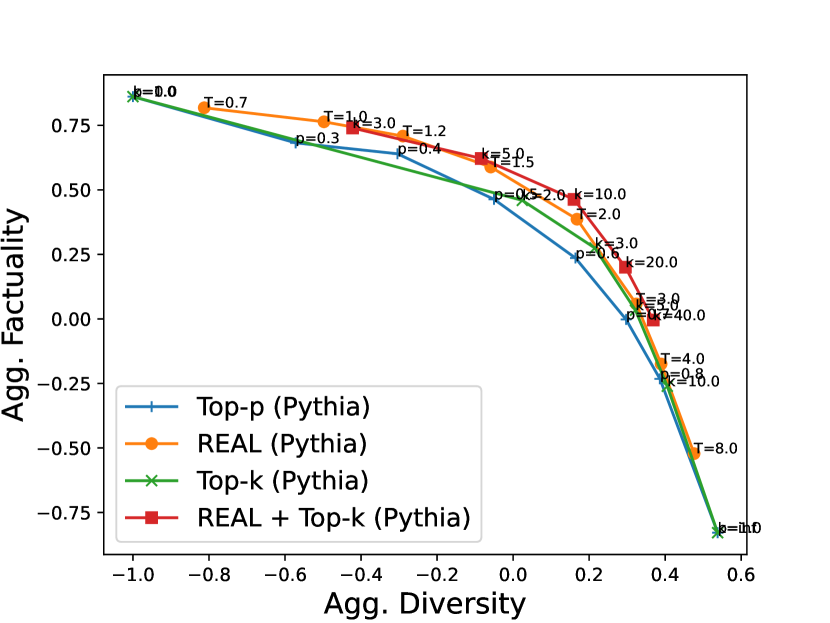
(h) REAL vs Top-$k$ Sampling

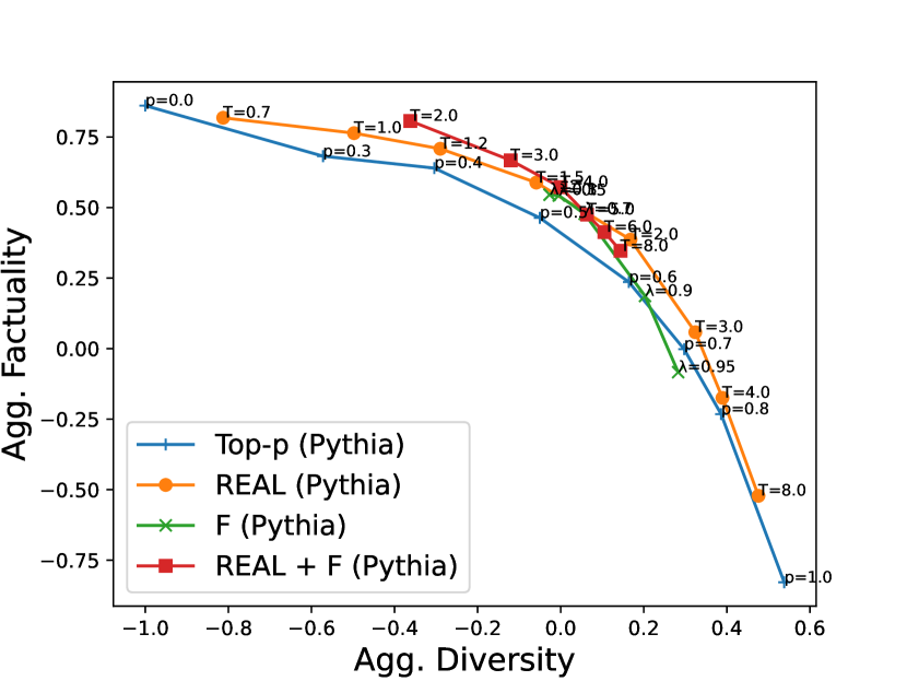
(i) REAL vs Factual (F) Sampling

Figure 12: Open-ended text generation performance comparison using FactualityPrompts. The same experiment setup of Figure 5 except that the factuality metrics and dist-2 are applied to 3 generated sentences rather than 1 generated sentence.

E.1 Evaluation on Longer Continuations

The evaluation code from FactualityPrompts only checks the factuality of the first generated sentence after the prompt. As the we generate more text, the hallucination problem is more likely to happen [58]. To see if our conclusions still hold for longer continuations, we evaluate the three generated sentences and plot the results in Figure 12. We can see that the overall trend is similar to the first-sentence results in Figure 5 and Figure 13, which suggests that our improvements are mostly not affected by the generation length.

(a) REAL vs Top-$k$ Sampling

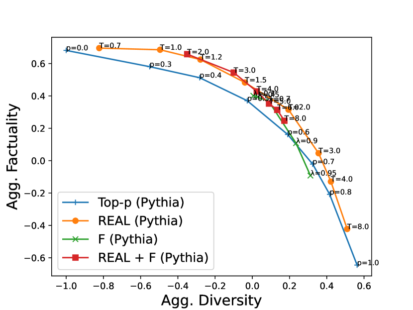
(b) REAL vs Factual (F) Sampling

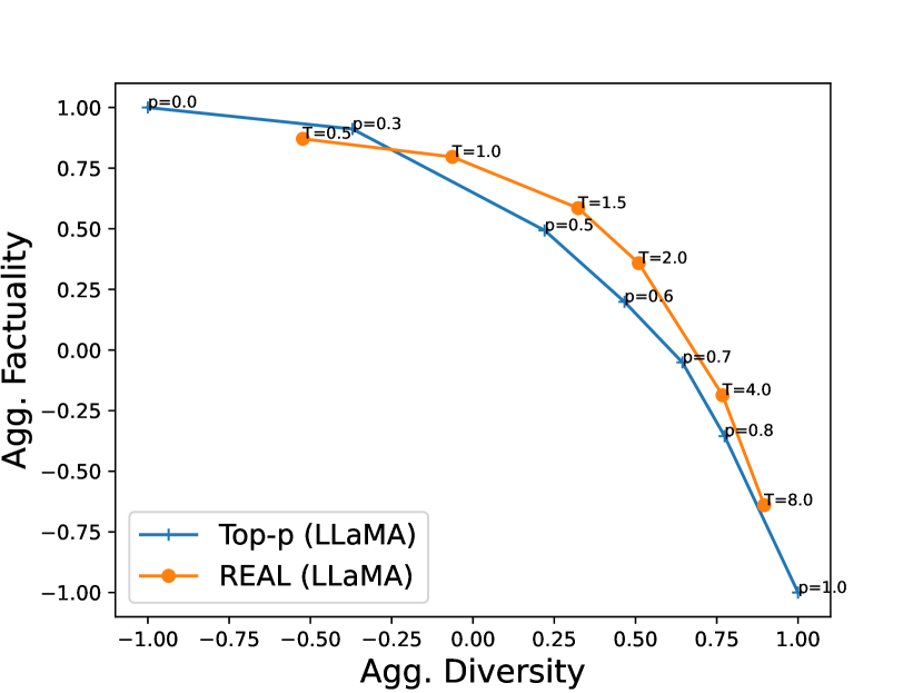
(c) Using OpenLLaMA-7b as the generation LLM and the THF model trained on Pythia.

Figure 13: Comparison of open-ended text generation methods in FactualityPrompts including top-$k$ [18] and factual (F) [27] sampling. We also conduct another out-of-domain evaluation for REAL sampling using OpenLLaMA-7b.

E.2 More Comparisons

Due to the page limit and clarity of the figures, we move some comparisons to this section. In addition to top-$k$ sampling [18], we also test the following generation methods:

• REAL + Top-$k$: Using the THF model to dynamically adjust the threshold in Top-$k$ sampling as $t_{c}^{k}=t^{k}\cdot\exp(-\hat{d}_{c}^{RE})$, where $t^{k}$ is a constant hyperparameter.

• F: Factual sampling (F) [27] exponentially reduces the $p$ value according to the distance to the last period. As suggested in the paper, we set the decay ratio $\lambda=0.9$ and fix the highest and the lowest sampling threshold to be the default values: $0.9$ and $0.3$, respectively. That is, $\hat{t}_{c}^{p}=\max(0.3,0.9\cdot 0.9^{x-1})$, where $x$ is the distance to the last period.

• REAL + F: Combining our methods with factual sampling using $\hat{t}_{c}^{p}=\max(0.3,0.9^{x-1})\cdot\exp(\frac{-\hat{d}_{c}^{RE}}{T})$.

• * (LLaMA): In the methods, we replace the Pythia 6.9B with OpenLLaMA2-7b [51, 14, 21] as the generation LLM, respectively. Notice that the THF model is still trained using the Pythia family.

Results: Figure 13 shows that top-$k$ outperforms top-$p$ sampling at the high diversity side while the factual (F) sampling outperforms top-$p$ sampling at the low diversity side. Notice that factual sampling relies on the heuristic/assumption that hallucination is more likely to happen near the end of the sentence. The assumption might not work well in some languages or applications such as code generation.

REAL sampling could be easily combined with these approaches and boost their performance at Figure 13(a) and Figure 13(b). In Figure 12(h) and Figure 12(i), the combinations are often significantly better than using REAL sampling alone.

Finally, similar to OPT 6.7B, our THF model trained on Pythia could still improve OpenLLaMA2 in Figure 13(c). Unlike OPT, we do not report the CD performance for OpenLLaMA2 because the smallest model in the family is too large (OpenLLaMA2-3b).

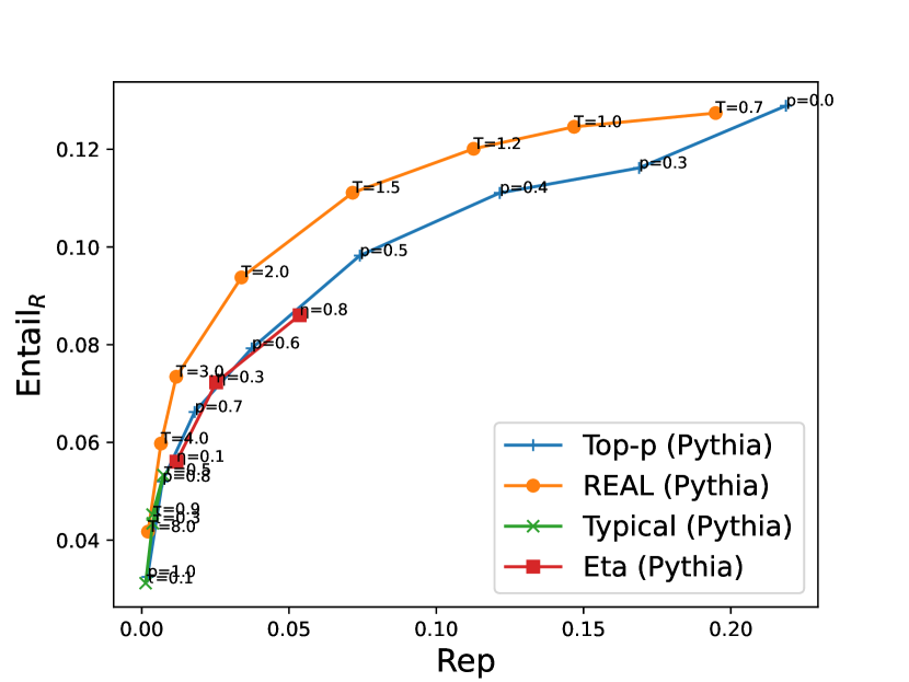
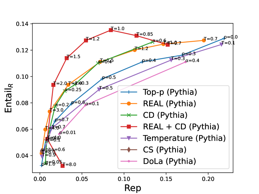
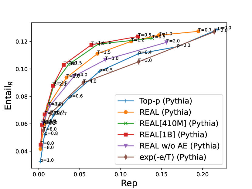
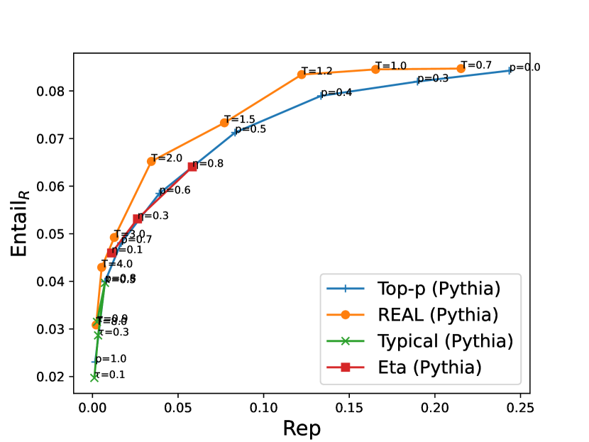
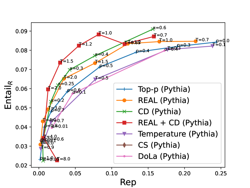
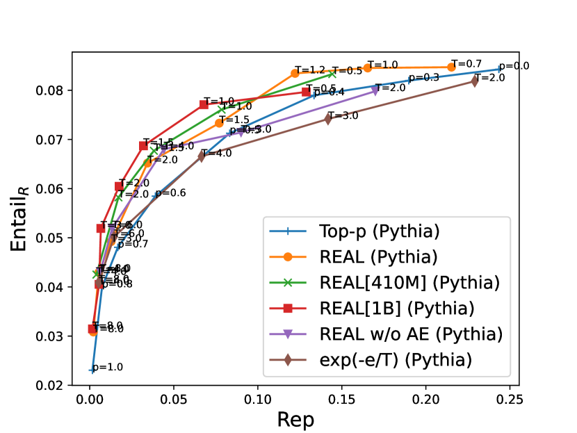
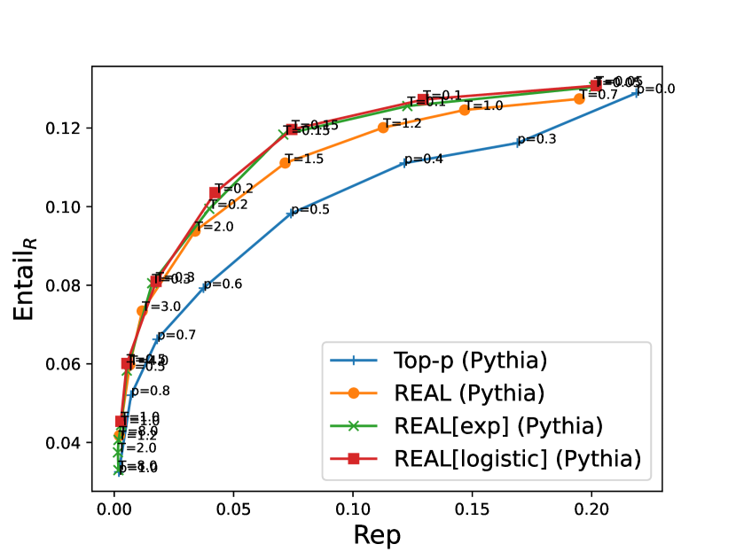
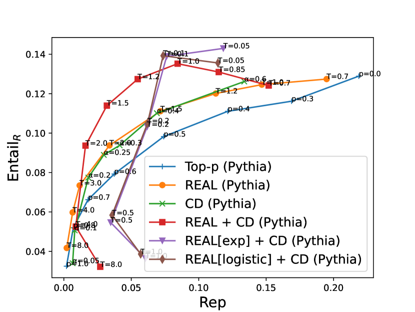
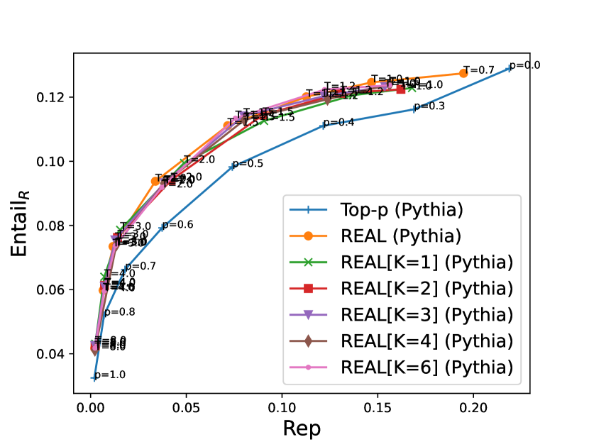
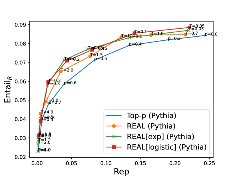
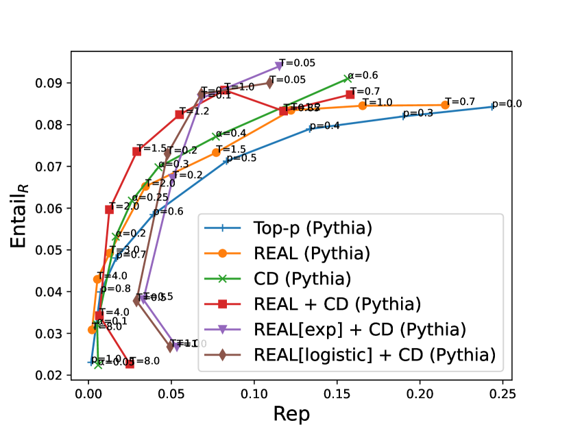
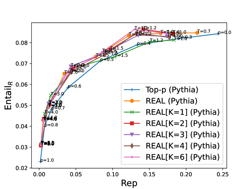
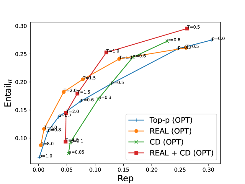
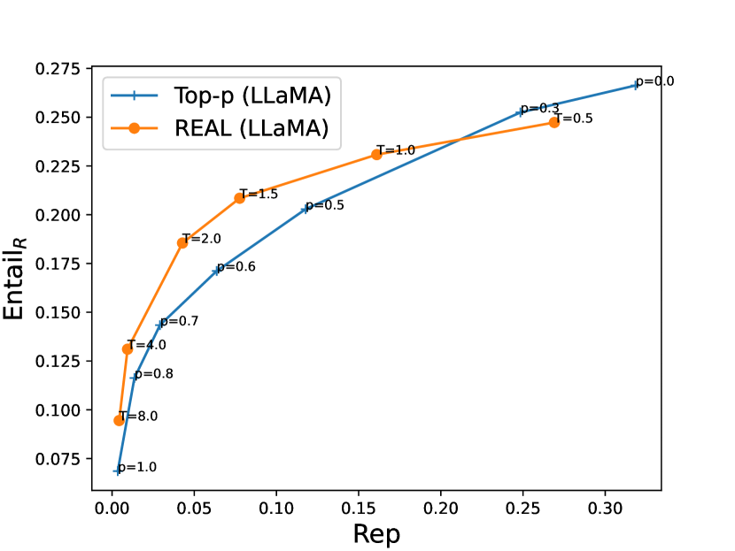
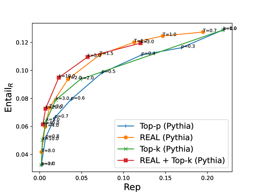
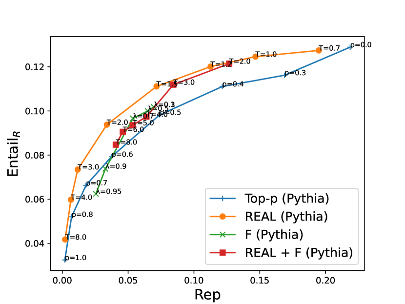
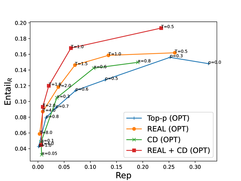
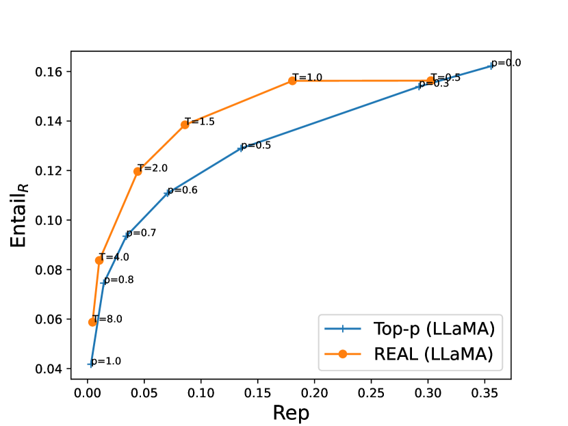
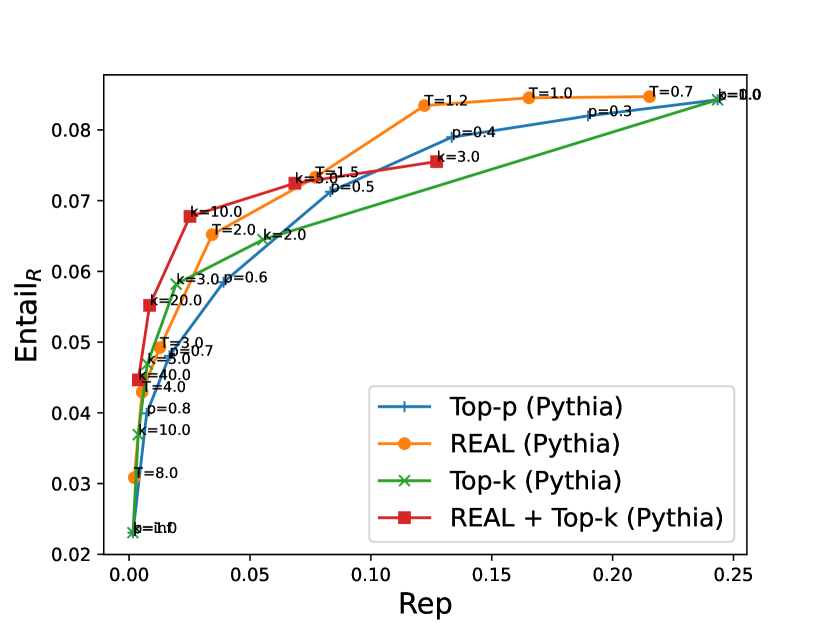
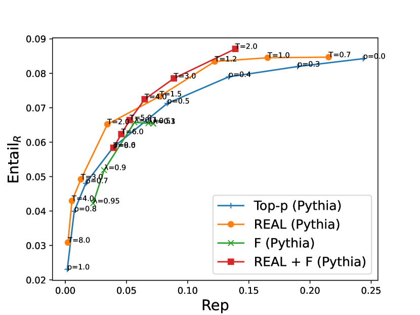
(a) REAL vs Thresholding Methods (Factual) (b) REAL vs Distribution Modifications (Factual) (c) Ablation (Factual) (d) REAL vs Thresholding Methods (Nonfactual) (e) REAL vs Distribution Modifications (Nonfactual) (f) Ablation (Nonfactual) (g) Different Parameterizations
(Factual) (h) Different Parameterizations
(Factual) (i) Different Polynomial Degrees
(Factual) (j) Different Parameterizations
(Nonfactual) (k) Different Parameterizations
(Nonfactual) (l) Different Polynomial Degrees
(Nonfactual) (m) OPT-6.7b (Factual) (n) OpenLLaMA-7b
(Factual) (o) REAL vs Top-k
(Factual) (p) REAL vs F (Factual) (q) OPT-6.7b (Nonfactual) (r) OpenLLaMA-7b
(Nonfactual) (s) REAL vs Top-k
(Nonfactual) (t) REAL vs F (Nonfactual)

Figure 14: The entailment ratio (Entail_R) versus repetition ratio (Rep). A lower repetition ratio is better, so the better methods are closer to the top-left corner. (Factual) in the captions means the prompt sentence is factual. The y-axis standard errors of every curve in this figure are 0.0015 on average and smaller than 0.005.

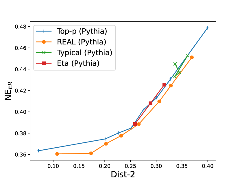
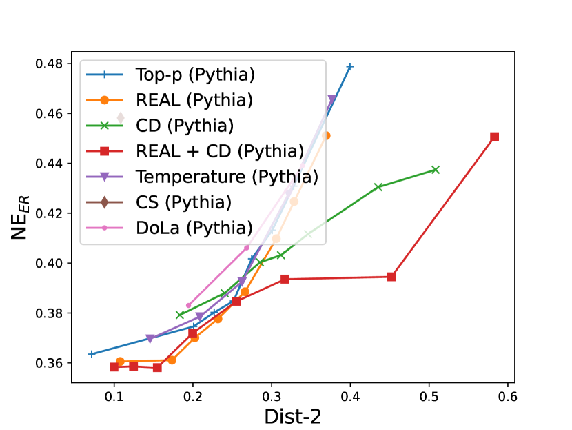
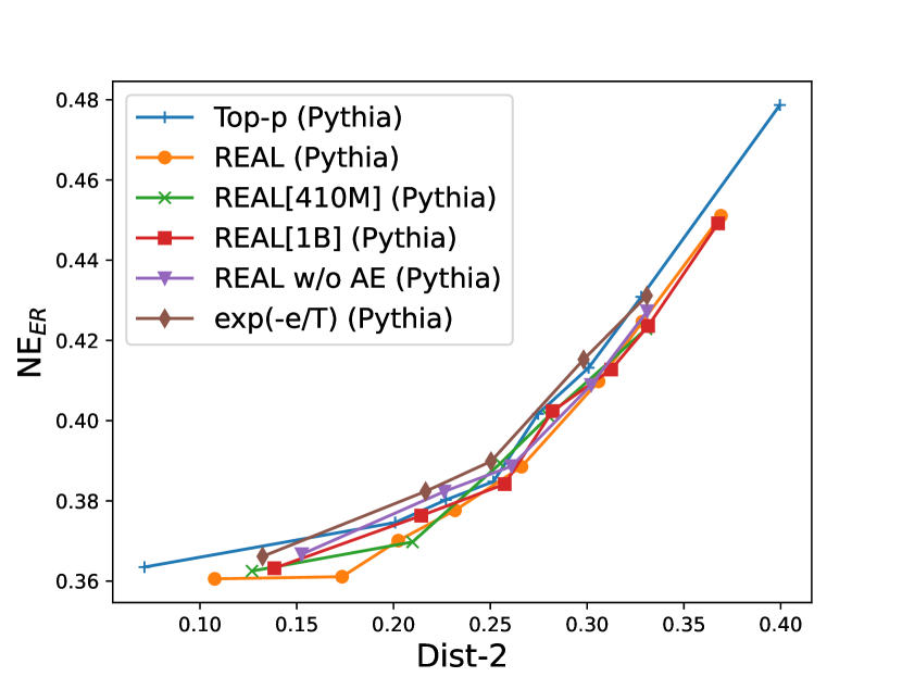
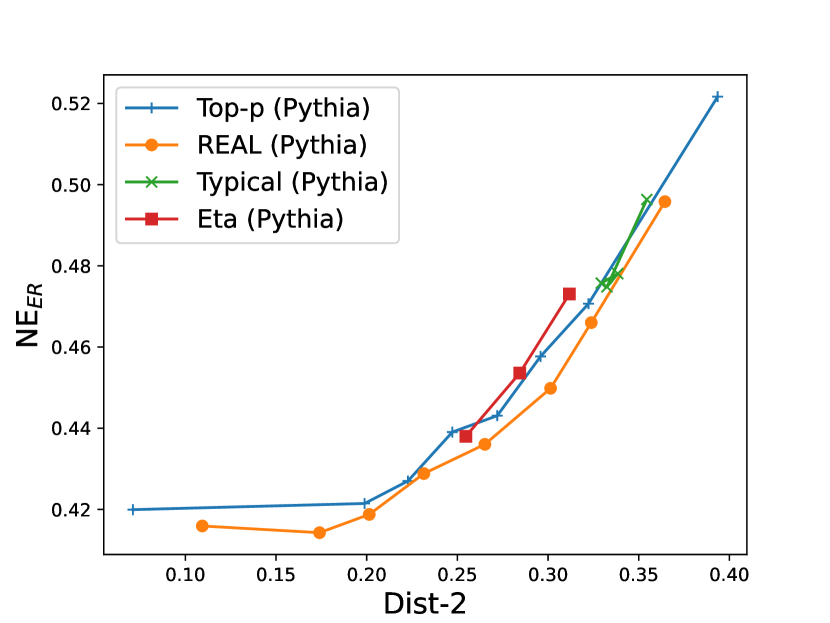
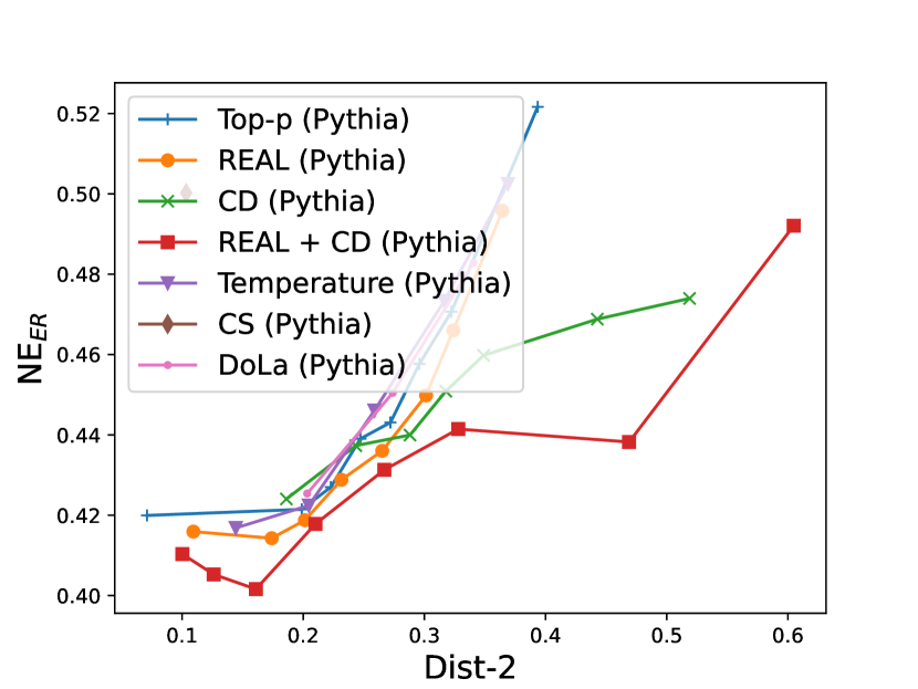
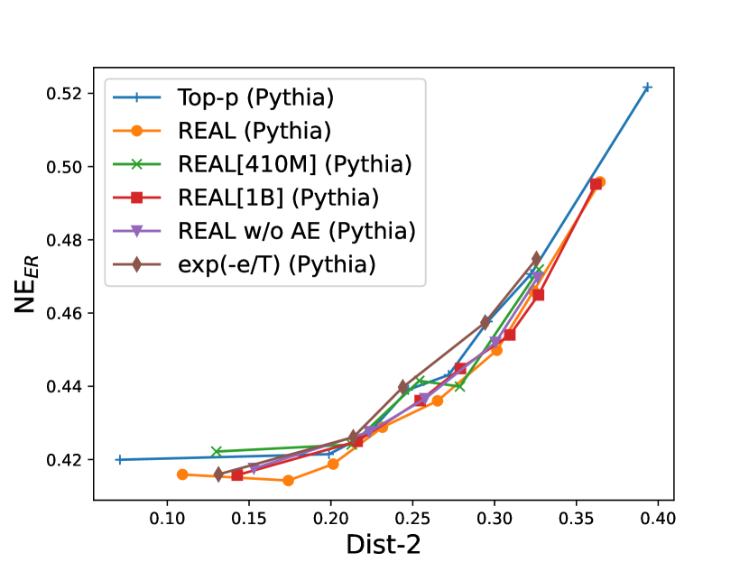
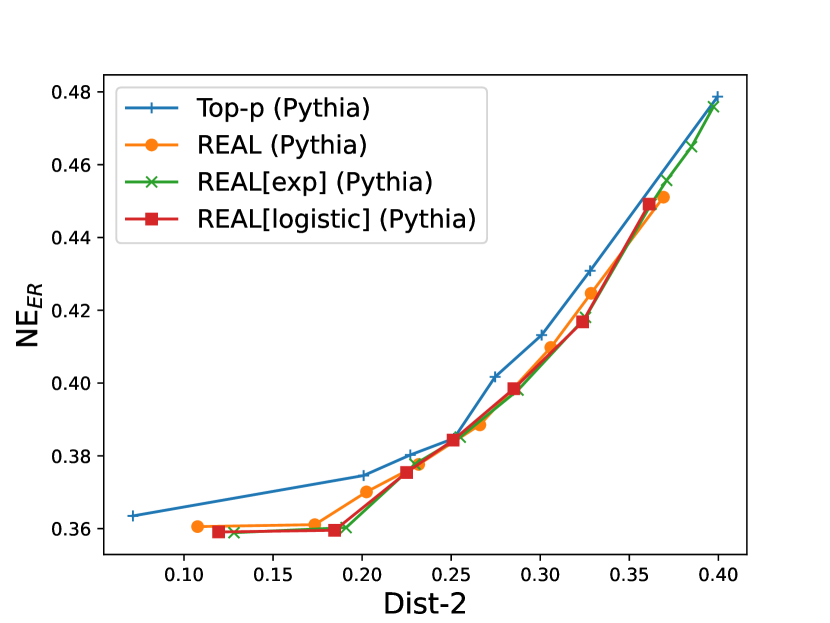
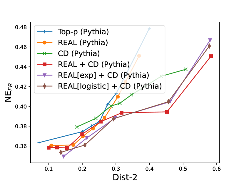
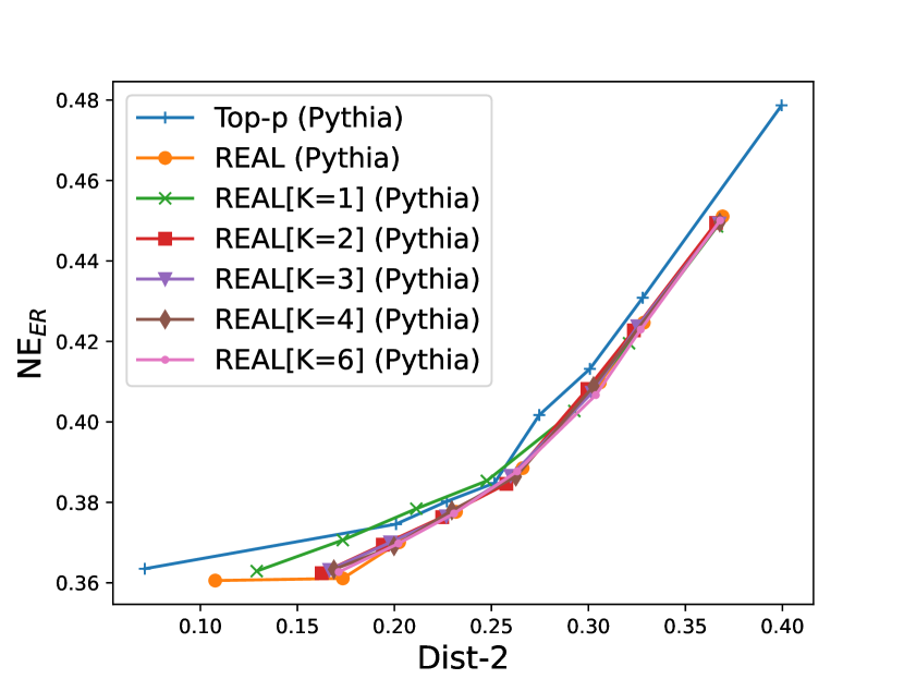
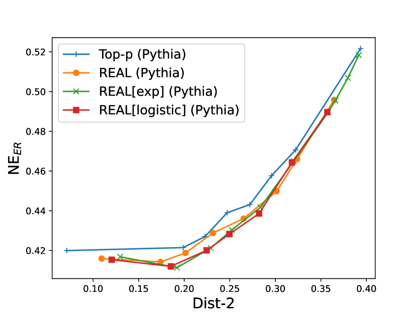
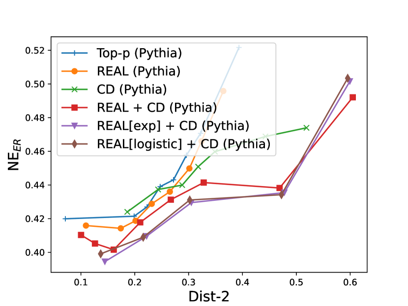
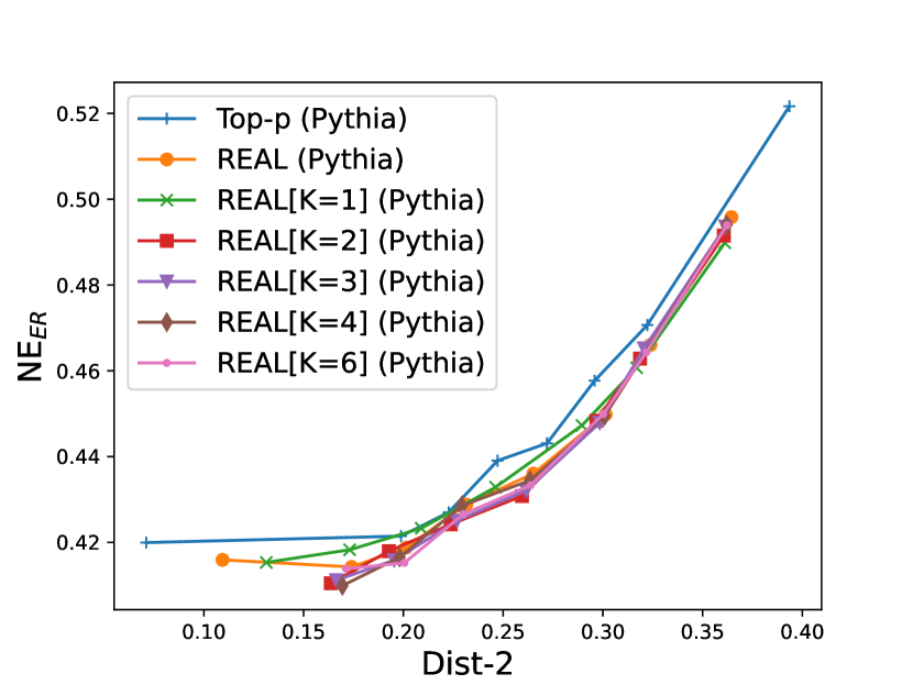
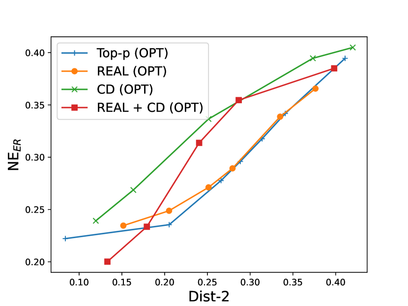
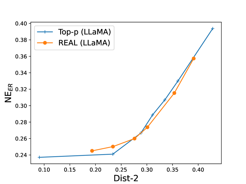
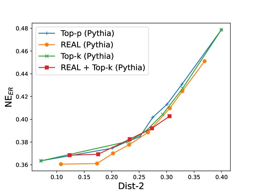
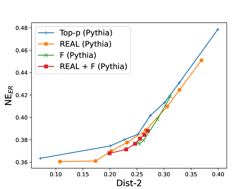
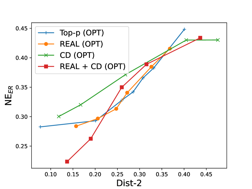
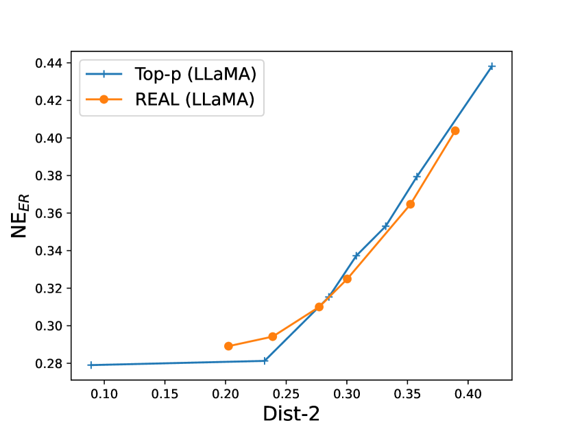
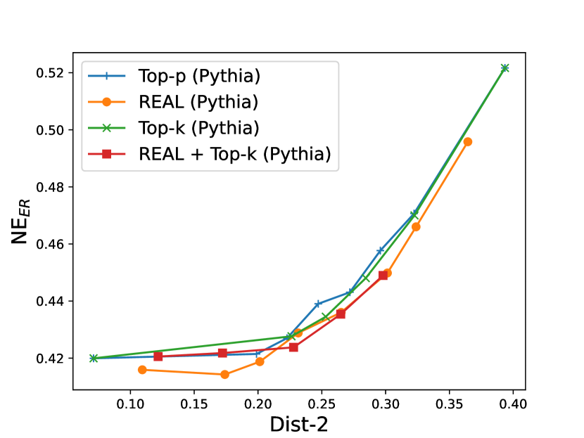
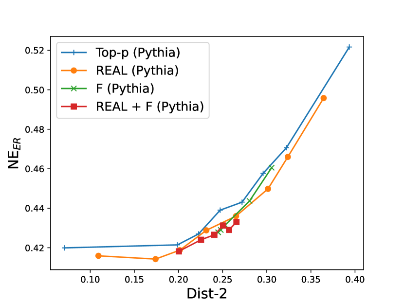
(a) REAL vs Thresholding Methods (Factual) (b) REAL vs Distribution Modifications (Factual) (c) Ablation (Factual) (d) REAL vs Thresholding Methods (Nonfactual) (e) REAL vs Distribution Modifications (Nonfactual) (f) Ablation (Nonfactual) (g) Different Parameterizations
(Factual) (h) Different Parameterizations
(Factual) (i) Different Polynomial Degrees
(Factual) (j) Different Parameterizations
(Nonfactual) (k) Different Parameterizations
(Nonfactual) (l) Different Polynomial Degrees
(Nonfactual) (m) OPT-6.7b (Factual) (n) OpenLLaMA-7b
(Factual) (o) REAL vs Top-k
(Factual) (p) REAL vs F (Factual) (q) OPT-6.7b (Nonfactual) (r) OpenLLaMA-7b
(Nonfactual) (s) REAL vs Top-k
(Nonfactual) (t) REAL vs F (Nonfactual)

Figure 15: The named entity error ratio (NE_ER) versus distinct bi-gram (Dist-2). Lower NE_ER is better, so the better methods are closer to the bottom-right corner. (Factual) in the captions means the prompt sentence is factual. We hide the hyperparameter values in the figures to avoid blocking the curves. The y-axis standard errors of every curve in this figure are 0.002 on average and smaller than 0.006.

E.3 Individual Metrics

We present the performances of entailment ratio (Entail_R) and repetition ratio (Rep) in Figure 14. We also present the performances of named entity error ratio (NE_ER) and distinct bi-gram (Dist-2) in Figure 15. In both figures, we separate the performances given factual prompts and nonfactual prompts. We can see that the overall trends are similar compared to Figure 5. The better scores for the nonfactual prompts show that our methods are less likely to propagate factual errors when generating the text [58]. Our improvements are larger in Figure 14. It suggests that our methods are especially effective in alleviating the repetition problem. Surprisingly, we observe that REAL sampling could be even slightly more factual than the greedy decoding (Top-$p$ with $t^{p}=0$), which is reported as the leftmost points in Figure 15(a) and Figure 15(d). This suggests greedy decoding might not always have less hallucination compared to the sampling.

E.4 Speed Comparison

Since the size of our 70M THF model is 100 times smaller than 7B LLM, the inference time of the THF model should be negligible if we parallelly run both the LLM and THF model at each decoding step. Without optimizing for speed, our current implementation simply runs the 70M THF model at every decoding step of LLM. In this naive implementation, the decoding time still only increases around 11% (from 7.46 to 8.29 seconds) when the batch size is 8 and the maximal number of tokens is 128.

Table 4: Human experiment and automatic metrics for FactualityPrompts.

	Human experiments (100 continuations)				Automatic Metrics (28k continuations) (%)
	Overall	Factuality	Informativeness	Fluency	Dist-2	Rep ($\downarrow$)	NEER ($\downarrow$)	EntailR
Top-$p$ ($p=0.6$)	2.55	2.15	3.46	4.01	27.466	3.736	40.171	7.925
REAL ($T=2.0$)	2.78	2.32	3.53	4.14	26.608	3.386	38.850	9.377
CD ($\alpha=0.3$)	2.84	2.47	3.61	4.08	28.511	4.143	40.031	9.380
REAL+CD ($T=1.5$)	2.86	2.48	3.64	4.09	25.505	3.193	38.462	11.394

E.5 Human Experiment for FactualityPrompts

In Table 4, we provide the average scores of each method. In the human experiment, we can see that the factuality improvements of REAL over Top-$p$ are larger than the improvements of REAL + CD over CD, while the order is reversed in the automatic metrics. It might be due to the relatively small testing set in the human experiment, or some factors that can be measured by human evaluation.

The average Pearson correlation between the two workers in every task is 23.5% for overall, 37.3% for factuality, 14.2% for informativeness, and 12.3% for fluency. Notice that we only change the truncation threshold in the sampling methods on top of the same generation LLM, so the generated next sentences are sometimes very similar. This makes workers sometimes hard to give different scores to different generations. We observe that the agreements of informativeness and fluency are low while their average absolute scores are high. One possible reason is that all generations have similarly good fluency, so workers tend to disagree about which ones are slightly less fluent.

Appendix F More Result Analyses

In Figure 5(b), we observe that REAL sampling could double the improvements of contrastive decoding (CD). One possible reason is that CD might reduce the diversity when there are many correct next tokens and REAL sampling could alleviate the problem. For example, in Figure 3 (b), the distributions of small LM could be slightly flatter version of LLM’s distribution. Then, CD could significantly reduce the probability of less likely options such as When and thus lead to lower diversity. REAL sampling could fix the problem by dynamically increasing the $p$ threshold to include more options.

In Figure 5(c), we observe that REAL w/o AE, whose $\hat{t}_{c}^{p}=\exp(\frac{-e_{c}(s_{N})}{T})$, performs better than Top-$p$ and exp(-e/T) sampling, whose $\hat{t}_{c}^{p}=\exp(\frac{-e_{c}^{\theta_{s_{N}}}}{T})$. We want to know if the improvement comes from the extra entropy information from the Pythia LLM family, so we use the THF model to predict the $e_{c}^{\theta_{s_{N}}}$ directly. The preliminary result in our validation set shows that REAL w/o AE performs similarly if we replace the $e_{c}(s_{N})$ with the direct prediction, so the improvement does not come from the entropy information of other smaller LLMs.

This is an interesting finding. We hypothesize that the improvement of REAL w/o AE comes from smoothing the LLM’s entropy $e_{c}^{\theta_{s_{N}}}$ by the prediction of the tiny model (e.g., the LLM might have very different entropies for the three similar context in Figure 4, while the tiny model tends to output the average of these entropies). That is, it is not a good strategy to select less lower probability tokens when the entropy of its distribution is high. Instead, it is better to ask the LLM to be more careful when the next token is generally hard to predict (e.g., being an entity name) regardless of LLM’s certainty to the next token.

Table 5: Creative writing experiment in an out-of-domain setting. The generation model is Pythia 6.9B and we measure the winning rate against Top-p sampling with $p=0.5$ using GPT3.5.

	Wining Rate using GPT3.5 (500 continuations)				(8k continuations)
	Fluency	Coherence	Likability	Overall	Dist-2	Rep ($\downarrow$)
Top-$p$ ($p=0.5$)	50	50	50	50	18.600	7.463
REAL ($T=1.8$)	53	53.4	52.6	52.6	17.952	4.563

Appendix G Human Experiment for Creative Writing in an Out-of-Domain Setting

Creative writing is not the focus of this paper because the hallucination problem is usually not serious in the tasks. Nevertheless, we still evaluate our methods on a story-writing task. In the task, the prompt is composed of three stories from the ROC story dataset [38] and the first two sentences from the fourth story. Then, we use different decoding methods to complete the fourth story.

Evaluating the creative writing is a subjective task. To save cost, we use gpt-3.5-turbo-0125 to compare the continuations of 500 ROC stories from REAL sampling and from top-$p$ sampling. In Table 5, we report the winning rate against the top-$p$ sampling.

Results: Overall, REAL is similar top-$p$ sampling even when our training data for the THF model (i.e., Wikipedia and OpenWebText) does not include too many short stories. This shows that REAL sampling could improve the factuality of top-$p$ sampling without sacrificing its creative writing ability.

Appendix H Impact Statements

REAL sampling has strong open-ended text generation performances without supervision. For example, typical [37] sampling, a state-of-the-art thresholding method, improves top-$p$ by 0.4% (4.13->4.15) based on the human evaluation scores in their Table 1, while REAL sampling improves top-$p$ by 9% (2.545->2.775) in Table 4. Furthermore, our method has a wide application on LLMs because we did not make any domain-specific assumptions and REAL sampling can be combined with other decoding methods to achieve further improvements. This suggests that our method can potentially improve most of the state-of-the-art LLMs such as GPT-4 in all the domains.

Low generation factuality/quality could incur negative societal implications. For example, LLM could generate a fake case for a lawyer to cite [36] or a code with some subtle bugs for a software engineer to use. Our hallucination forecasting model could be used to give users better hallucination warning by improving the current token highlighting based on its entropy or probability (similar to what we did in Figure 6).

Low generation diversity also prevents the users from knowing different perspectives on a question and might increase the polarization of society. Thus, increasing both factuality and diversity could bring positive social impacts. Our unsupervised training methods could also bring the above benefits to other languages more easily. Nevertheless, increasing the factuality might also make it harder to distinct AI-generated text from human-written text and thus lead to some social problems. Discussing these potential social benefits and harms is out of the scope of this paper.

Appendix I Limitations and Future Work

We assume the target LLM family has models with different sizes. Although it is not always the case, our experiments show that the THF models trained in Pythia could still help OPT and OpenLLaMA, which suggests the existence of an universal THF model that could be generalized to the other LLM families without models with different sizes.

To motivate/explain our method, we assume that there is an ideal next-token distribution and the infinitely large LLM that can output this ideal distribution. Hence, the entropy of the ideal next-token distribution $e^{AE}_{c}$ exists. Nevertheless, without the assumption, we still know that the entropy of a larger LLM should be a better estimation of the inherent uncertainty, so we extrapolate the existing entropy decay curves to estimate the entropy of a very large LLM. Therefore, the theoretical existence of $e^{AE}_{c}$ does not affect the empirical/practical value of our extrapolation and our derivation in Theorem 3.1.

The unsupervised nature of REAL sampling makes it applicable to many domains and applications. For example, we could apply it to larger LLM. As shown in Figure 6, the entropy from 6.9B LLM is still very far away from asymptotic entropy, so we should get much more accurate estimations when we use a even larger LLM. We could use it to improve the code generation [31] or combine REAL sampling with the prompting methods that require both diversity and factuality [56, 4, 57, 40] or the hallucination reduction methods for specific applications [53, 35, 9, 45]. We could also use the THF model to improve the factuality/effectiveness/efficiency of beam search  [55, 52].

There are also several potential improvements for the THF model and REAL sampling. For example, our current ways of combining REAL sampling and other decoding methods are very simple. We could study how to better integrate these decoding methods. Moreover, we want to better support the off-the-shelf usage of the THF model. In Figure 5(c), we can see that the same temperature $T$ corresponds to two very different diversities for REAL and REAL (410M) and should be normalized based on the average RE ($\hat{d}_{c}^{RE}$). Besides, we can train a model that predicts the entropies of multiple LLM families to reduce the performance degradation in the out-of-domain transfer setting (e.g., training on Pythia and testing on OPT). In industry, running two models with very different sizes together might induce some engineering challenges or synchronization issues. Therefore, we can try to integrate the THF model with LLMs. One possible approach is to use the prediction of the THF model as a noisy signal to find the hallucination patterns of the hidden state as Burns et al. [7], Li et al. [29], Chuang et al. [13] did.

Appendix J Why does the Entropy Decay as the Model Size Increases?

First, in Figure 2, we empirically observe that the average entropy across our Wikipedia validation set (around 9M tokens) steadily decreases as the model size increases. Furthermore, there are 90.2% contexts given which the smallest Pythia LM (70M) has a larger next-token entropy compared to Pythia LLM (6.9B). We visualize some of the decay curves in Figure 6.

Intuitively speaking, a small language model is less likely to learn the ideal distribution, so it tends to put higher probabilities on more words so that it won’t receive a large penalty from the cross-entropy loss. Since its output distribution is closer to a uniform distribution, the entropy is higher.

We can also provide a more formal explanation by treating a smaller LLM as a n-gram LM with a smaller n. To simplify our explanation, let’s just assume our vocabulary is A,B,C and we want to show the average entropy 1-gram LM is larger than the average entropy 2-gram LM, which predicts the next word just based on one context word. Let’s denote the probability of seeing the word x as P(x) and the probability of seeing the word y given the context x is P(y|x). Since the entropy function is a concave function, we know that entropy of 2-gram LM = $\sum_{x=A,B,C}P(x)Ent(P(y|x))\leq Ent(\sum_{x=A,B,C}P(y|x)P(x))$ = the entropy of 1-gram LM. The intuitive explanation of this proof is that the probability distribution of 1-gram LM merges the 3 distributions of 2-gram LM, and merging distributions would lead to a higher entropy overall. We can easily generalize the above proof to show that the average entropy of n-gram LM is always larger than the average entropy of (n+1)-gram LM.

Appendix K Method Details

In open-ended text generation, we empirically observe that the RE $\hat{d}_{c}^{RE}$ gradually decreases as the context length increases because the LLM tends to be more certain about the next token given a long context. To avoid the systematic shift of $\hat{t}_{c}^{p}$, we only input the last $40$ tokens into the THF model. This truncation also further reduces the computational cost for a long context input and stablize the estimation of the curve parameters by limiting the prediction power of the tiny THF model [30].

We train our models using Wikipedia 2021 and OpenWebText [43]. In the training corpus, we first compute the entropies of each word using the Pythia with sizes 70M, 160M, 410M, 1B, 1.4B, 2.8B, and 6.9B. When computing the Log(model size), we use the number of parameters after excluding the token embeddings. We set the highest degree of our fractional polynomial $K=10$ by default and fine-tune the pretrained Pythia 70M for 3 epochs to predict their entropy decay curves. We set the learning rate as $5e-5$ and warm-up step as $100$. Furthermore, we initialize all values in the weight and bias of the linear layer before the final exponential layer with $0$ to prevent our exponential layer from causing too large gradients at the beginning of training.

We download the Wikipedia from http://medialab.di.unipi.it/wiki/Wikipedia_Extractor and download OpenWebText [43] from https://github.com/jcpeterson/openwebtext (GPL-3.0 license). We only use the first 5M lines of both datasets (around 5.6% of text) to accelerate our training because our preliminary studies show that our performance is not sensitive to the training corpus.

During training, the maximal length of context is $1024$ to ensure that the THL model can handle the long context in hallucination detection. We set the batch size to be $128$ for 70M model and $32$ for 410M model based on the limit of our GPU memory. Our preliminary experiments show that the performances of text generation and hallucination detection are not sensitive to these hyperparameters.

Appendix L Experiment Details

In our experiments, we always append a space at the beginning of the context for all generation LLMs due to the preference of LM tokenizer. All the training and experiments are done by 8 NVIDIA V100 32GB GPUs. Our code is built on Huggingface.

L.1 Details for Open-Ended Text Generation

For contrastive decoding (CD) [30], we fix the temperature for the amateur model to be $1$ and choose the smallest model in the LLM family as the amateur model (i.e., Pythia 70M in CD and OPT-125m in CD (OPT)). To make the comparison fair, we use sampling rather than beam search proposed in Li et al. [30]. For DoLa [13], we try two layer subsets suggested in the paper: 0,2,4,6,8,10,12,14,32 and 16,18,20,22,24,26,28,30,32. We report the results of the former one because of its much better performance than the later one.

The maximal length of the continuation is set as $128$. To allow the batch decoding during inference, we append $<$eos$>$ sequences before the input prompts. When we compute Entail_Rn, NE_ERn, Dist-2_n, and Rep_n, we separate the max-min normalization for each LLM generation model and each prompt type (e.g., The decoding method for Pythia, OPT, or OpenLLaMA that achieve the highest Entail_R given the factual prompts will all receive 1 in the Entail_Rn metric for factual prompts).

L.2 Details for Human Experiments

After having generated continuations from different methods in FactualityPrompts, we first exclude the continuations that cause the difficulties in comparing the factuality, including the same continuations from different methods, the continuations that are less than 10 characters, and the continuations that mention “External links”. For the story completion, we only keep the responses whose lengths are between 50-1000 characters. Then, we select the remaining top 100 testing factual prompts based on the original order of FactualityPrompts and randomly select 100 prompting stories.

We collaborate with a list of MTurk workers in multiple projects, so their annotation quality is much higher than the average MTurk workers. Then, we further manually filter MTurk workers based on the supporting URL and statements/reasons they provided. We control the hourly wage of these trusted MTurk workers to be around $14 and provide $2.2 reward for each task in FactualityPrompts and $1.5 reward for each task in story generation.

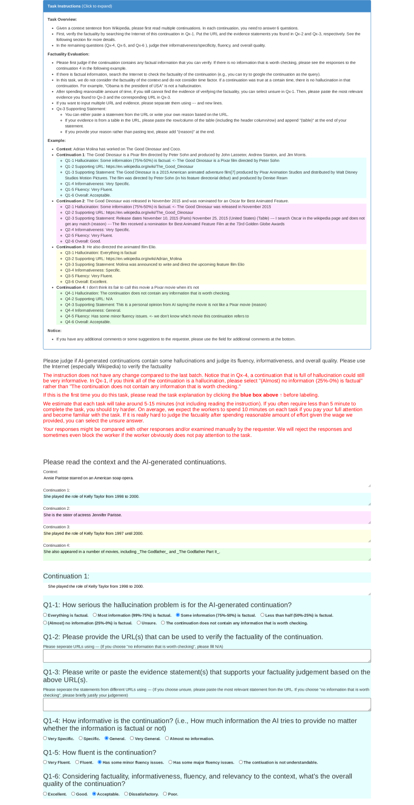
Figure 16: The MTurk template for our human experiment.

In each task, the order of the text generated by all methods is randomized. In FactualityPrompts, the factuality score 5 means no hallucination, and the score 1 means less than 25% of the continuation is factual. We allow the workers to select the “unsure” option if they really cannot find the relevant statement from the Internet and we also allow the workers to select “no information that is worth checking” option because the 7B LLM sometimes states their own opinions. We treat both options as score 1 in our evaluation. Please see Figure 16 for more details of our MTurk task.

L.3 Details for Hallucination Detection

Factor creates nonfactual sentences by revising the factual sentences given a context using ChatGPT, HaDes provides human labels on the phrases infilled by BERT, and TF ext mostly uses templates and tables in different topics to create the factual and nonfactual sentences. The hallucination datasets are created using very different methods and none of the input text is not from Pythia. Our improvements highlight the generalization capability of our model and its potential to improve the applications that leverage the perplexity and entropy measurement (e.g., hallucination detection, AI-generated text detection, and creativity measurement).

Notice that the main purpose of this experiment is to demonstrate the potential of using the THF model to improve unsupervised hallucination detection in general rather than achieving state-of-the-art performances. Muhlgay et al. [39] have shown that larger LLMs can better detect the hallucination. In this experiment, all the features are derived from Pythia LLMs with a size smaller than 7B without any additional training or supervision (e.g., supervised training, instruction finetuning, RLHF [42], distillation, etc), so it might not work better than directly fine-tuning a model for a particular hallucination detection dataset or a more advanced/larger LLM.

We use the training and testing split in HaDes [32]. For Factor and TF ext, we split each subset into equally large training set and testing set. The maximal depth of the random forest is set as $5$. For Hades, we use only the perplexity and the entropy of the first token in the input phrase as our features, which works better than averaging the perplexities and entropies of all the tokens in the input phrase. In the last two rows of Table 2, we use the code of HaDes [32] to perform exhaustive feature selection based on the testing scores, so we can view the results as validation scores. In Hades and TF ext, we choose the best feature set based on AUC and in Factor, we select features using 1-4 ACC.

L.4 Details for Creative Writing Experiments

Chiang and Lee [12] suggest that asking ChatGPT to rate first and give explanation next could increase the quality of the scores. Following the suggestion, we design our prompt and report it in Section L.4. To avoid the position bias in the evaluation, we alternatively assign the generation from REAL sampling and from top-$p$ sampling to be story continuation A.

You are an English writing expert and you can compare and evaluate two continuations on these metrics with the following definitions -

1. Fluency: Which continuation has better writing and grammar comparitively?

2. Coherence: Which continuation has a better logical flow and the writing fits together with respect to the plot?

3. Likability: Which continuation is more interesting and enjoyable to read?

You will be given two continuations - continuation A and continuation B.

Specify which continuation you prefer for each metric by responding with just the letter “A” or “B” followed by a hyphen and two line justifications for your preference.

Assign an overall winner continuation as the letter “A” or “B” based on the category wins and provide two line justifications.

IMPORTANT - DO NOT GIVE ANY OTHER TEXT APART FROM THE METRICS, PREFERENCE, AND JUSTIFICATIONO.

EXAMPLE OUTPUT 1:

Fluency: B

A: A has some complex sentences that are difficult to follow, with occasional grammatical errors.

B: B is well-written with minor grammatical mistakes and clear sentence structures.

Coherence: B

A: The plot of A is somewhat confusing and disjointed, especially with the sudden introduction of an old sage.

B: B maintains a coherent narrative, with each event logically building on the previous one, enhancing the continuation’s flow.

Likability: B

A: A is heartfelt but its erratic narrative structure detracts from its overall appeal.

B: B is compelling and maintains consistent character development, making it more enjoyable and engaging.

Overall Winner: B

A: A is moderately fluent, coherent, and interesting.

B: B is perfect except for some minor grammar issues.

EXAMPLE OUTPUT 2:

Fluency: A

A: A has a few minor grammatical issues, but overall, it demonstrates strong control of language.

B: B is well-written but has slightly more noticeable issues in grammar and sentence structure.

Coherence: A

A: B has a strong coherence, effectively conveying the progression of events.

B: A maintains a consistent and engaging narrative flow, though some parts are a bit abstract.

Likability: A

A: B’s realistic and emotional narrative is likely to resonate more with a wide range of readers.

B: A is imaginative and intriguing, but its abstract nature might not appeal to all readers.

Overall Winner: A

A: A is very good and it would be better if it can be more interesting.

B: B is too abstract to be interesting.

Context: {Context}

Continuation A: {Context} {Story Continuation A}

Continuation B: {Context} {Story Continuation B}

NeurIPS Paper Checklist

1. Claims

2. Question: Do the main claims made in the abstract and introduction accurately reflect the paper’s contributions and scope?

3. Answer: [Yes]

4. Justification: We claim that the proposed REAL sampling improves both factuality and diversity. The claim is supported by various experiments and analyses.

5. Guidelines:

   • The answer NA means that the abstract and introduction do not include the claims made in the paper.

   • The abstract and/or introduction should clearly state the claims made, including the contributions made in the paper and important assumptions and limitations. A No or NA answer to this question will not be perceived well by the reviewers.

   • The claims made should match theoretical and experimental results, and reflect how much the results can be expected to generalize to other settings.

   • It is fine to include aspirational goals as motivation as long as it is clear that these goals are not attained by the paper.

6. Limitations

7. Question: Does the paper discuss the limitations of the work performed by the authors?

8. Answer: [Yes]

9. Justification: Please see Appendix I.

10. Guidelines:

    • The answer NA means that the paper has no limitation while the answer No means that the paper has limitations, but those are not discussed in the paper.

    • The authors are encouraged to create a separate "Limitations" section in their paper.

    • The paper should point out any strong assumptions and how robust the results are to violations of these assumptions (e.g., independence assumptions, noiseless settings, model well-specification, asymptotic approximations only holding locally). The authors should reflect on how these assumptions might be violated in practice and what the implications would be.

    • The authors should reflect on the scope of the claims made, e.g., if the approach was only tested on a few datasets or with a few runs. In general, empirical results often depend on implicit assumptions, which should be articulated.

    • The authors should reflect on the factors that influence the performance of the approach. For example, a facial recognition algorithm may perform poorly when image resolution is low or images are taken in low lighting. Or a speech-to-text system might not be used reliably to provide closed captions for online lectures because it fails to handle technical jargon.

    • The authors should discuss the computational efficiency of the proposed algorithms and how they scale with dataset size.

    • If applicable, the authors should discuss possible limitations of their approach to address problems of privacy and fairness.

    • While the authors might fear that complete honesty about limitations might be used by reviewers as grounds for rejection, a worse outcome might be that reviewers discover limitations that aren’t acknowledged in the paper. The authors should use their best judgment and recognize that individual actions in favor of transparency play an important role in developing norms that preserve the integrity of the community. Reviewers will be specifically instructed to not penalize honesty concerning limitations.

11. Theory Assumptions and Proofs

12. Question: For each theoretical result, does the paper provide the full set of assumptions and a complete (and correct) proof?

13. Answer: [Yes]

14. Justification: Please see Appendix B

15. Guidelines:

    • The answer NA means that the paper does not include theoretical results.

    • All the theorems, formulas, and proofs in the paper should be numbered and cross-referenced.

    • All assumptions should be clearly stated or referenced in the statement of any theorems.

    • The proofs can either appear in the main paper or the supplemental material, but if they appear in the supplemental material, the authors are encouraged to provide a short proof sketch to provide intuition.

    • Inversely, any informal proof provided in the core of the paper should be complemented by formal proofs provided in appendix or supplemental material.

    • Theorems and Lemmas that the proof relies upon should be properly referenced.

16. Experimental Result Reproducibility

17. Question: Does the paper fully disclose all the information needed to reproduce the main experimental results of the paper to the extent that it affects the main claims and/or conclusions of the paper (regardless of whether the code and data are provided or not)?

18. Answer: [Yes]

19. Justification: Please see Appendix K and Appendix L.

20. Guidelines:

    • The answer NA means that the paper does not include experiments.

    • If the paper includes experiments, a No answer to this question will not be perceived well by the reviewers: Making the paper reproducible is important, regardless of whether the code and data are provided or not.

    • If the contribution is a dataset and/or model, the authors should describe the steps taken to make their results reproducible or verifiable.

    • Depending on the contribution, reproducibility can be accomplished in various ways. For example, if the contribution is a novel architecture, describing the architecture fully might suffice, or if the contribution is a specific model and empirical evaluation, it may be necessary to either make it possible for others to replicate the model with the same dataset, or provide access to the model. In general. releasing code and data is often one good way to accomplish this, but reproducibility can also be provided via detailed instructions for how to replicate the results, access to a hosted model (e.g., in the case of a large language model), releasing of a model checkpoint, or other means that are appropriate to the research performed.

    • While NeurIPS does not require releasing code, the conference does require all submissions to provide some reasonable avenue for reproducibility, which may depend on the nature of the contribution. For example

      1. If the contribution is primarily a new algorithm, the paper should make it clear how to reproduce that algorithm.

      2. If the contribution is primarily a new model architecture, the paper should describe the architecture clearly and fully.

      3. If the contribution is a new model (e.g., a large language model), then there should either be a way to access this model for reproducing the results or a way to reproduce the model (e.g., with an open-source dataset or instructions for how to construct the dataset).

      4. We recognize that reproducibility may be tricky in some cases, in which case authors are welcome to describe the particular way they provide for reproducibility. In the case of closed-source models, it may be that access to the model is limited in some way (e.g., to registered users), but it should be possible for other researchers to have some path to reproducing or verifying the results.

21. Open access to data and code

22. Question: Does the paper provide open access to the data and code, with sufficient instructions to faithfully reproduce the main experimental results, as described in supplemental material?

23. Answer: [No]

24. Justification: We plan to publicly release all our code after the paper is accepted.

25. Guidelines:

    • The answer NA means that paper does not include experiments requiring code.

    • Please see the NeurIPS code and data submission guidelines (https://nips.cc/public/guides/CodeSubmissionPolicy) for more details.

    • While we encourage the release of code and data, we understand that this might not be possible, so “No” is an acceptable answer. Papers cannot be rejected simply for not including code, unless this is central to the contribution (e.g., for a new open-source benchmark).

    • The instructions should contain the exact command and environment needed to run to reproduce the results. See the NeurIPS code and data submission guidelines (https://nips.cc/public/guides/CodeSubmissionPolicy) for more details.

    • The authors should provide instructions on data access and preparation, including how to access the raw data, preprocessed data, intermediate data, and generated data, etc.

    • The authors should provide scripts to reproduce all experimental results for the new proposed method and baselines. If only a subset of experiments are reproducible, they should state which ones are omitted from the script and why.

    • At submission time, to preserve anonymity, the authors should release anonymized versions (if applicable).

    • Providing as much information as possible in supplemental material (appended to the paper) is recommended, but including URLs to data and code is permitted.

26. Experimental Setting/Details

27. Question: Does the paper specify all the training and test details (e.g., data splits, hyperparameters, how they were chosen, type of optimizer, etc.) necessary to understand the results?

28. Answer: [Yes]

29. Justification: Please see Section 4.1 and Appendix L.

30. Guidelines:

    • The answer NA means that the paper does not include experiments.

    • The experimental setting should be presented in the core of the paper to a level of detail that is necessary to appreciate the results and make sense of them.

    • The full details can be provided either with the code, in appendix, or as supplemental material.

31. Experiment Statistical Significance

32. Question: Does the paper report error bars suitably and correctly defined or other appropriate information about the statistical significance of the experiments?

33. Answer: [Yes]

34. Justification: Please see the captions of Table 1, Figure 14(t), and Figure 15(t). We put them into the caption for the clarity of the figures and table.

35. Guidelines:

    • The answer NA means that the paper does not include experiments.

    • The authors should answer "Yes" if the results are accompanied by error bars, confidence intervals, or statistical significance tests, at least for the experiments that support the main claims of the paper.

    • The factors of variability that the error bars are capturing should be clearly stated (for example, train/test split, initialization, random drawing of some parameter, or overall run with given experimental conditions).

    • The method for calculating the error bars should be explained (closed form formula, call to a library function, bootstrap, etc.)

    • The assumptions made should be given (e.g., Normally distributed errors).

    • It should be clear whether the error bar is the standard deviation or the standard error of the mean.

    • It is OK to report 1-sigma error bars, but one should state it. The authors should preferably report a 2-sigma error bar than state that they have a 96% CI, if the hypothesis of Normality of errors is not verified.

    • For asymmetric distributions, the authors should be careful not to show in tables or figures symmetric error bars that would yield results that are out of range (e.g. negative error rates).

    • If error bars are reported in tables or plots, The authors should explain in the text how they were calculated and reference the corresponding figures or tables in the text.

36. Experiments Compute Resources

37. Question: For each experiment, does the paper provide sufficient information on the computer resources (type of compute workers, memory, time of execution) needed to reproduce the experiments?

38. Answer: [Yes]

39. Justification: Please see Appendix L.

40. Guidelines:

    • The answer NA means that the paper does not include experiments.

    • The paper should indicate the type of compute workers CPU or GPU, internal cluster, or cloud provider, including relevant memory and storage.

    • The paper should provide the amount of compute required for each of the individual experimental runs as well as estimate the total compute.

    • The paper should disclose whether the full research project required more compute than the experiments reported in the paper (e.g., preliminary or failed experiments that didn’t make it into the paper).

41. Code Of Ethics

42. Question: Does the research conducted in the paper conform, in every respect, with the NeurIPS Code of Ethics https://neurips.cc/public/EthicsGuidelines?

43. Answer: [Yes]

44. Justification: Please see Appendix H.

45. Guidelines:

    • The answer NA means that the authors have not reviewed the NeurIPS Code of Ethics.

    • If the authors answer No, they should explain the special circumstances that require a deviation from the Code of Ethics.

    • The authors should make sure to preserve anonymity (e.g., if there is a special consideration due to laws or regulations in their jurisdiction).

46. Broader Impacts

47. Question: Does the paper discuss both potential positive societal impacts and negative societal impacts of the work performed?

48. Answer: [Yes]

49. Justification: Please see Appendix H.

50. Guidelines:

    • The answer NA means that there is no societal impact of the work performed.

    • If the authors answer NA or No, they should explain why their work has no societal impact or why the paper does not address societal impact.

    • Examples of negative societal impacts include potential malicious or unintended uses (e.g., disinformation, generating fake profiles, surveillance), fairness considerations (e.g., deployment of technologies that could make decisions that unfairly impact specific groups), privacy considerations, and security considerations.

    • The conference expects that many papers will be foundational research and not tied to particular applications, let alone deployments. However, if there is a direct path to any negative applications, the authors should point it out. For example, it is legitimate to point out that an improvement in the quality of generative models could be used to generate deepfakes for disinformation. On the other hand, it is not needed to point out that a generic algorithm for optimizing neural networks could enable people to train models that generate Deepfakes faster.

    • The authors should consider possible harms that could arise when the technology is being used as intended and functioning correctly, harms that could arise when the technology is being used as intended but gives incorrect results, and harms following from (intentional or unintentional) misuse of the technology.

    • If there are negative societal impacts, the authors could also discuss possible mitigation strategies (e.g., gated release of models, providing defenses in addition to attacks, mechanisms for monitoring misuse, mechanisms to monitor how a system learns from feedback over time, improving the efficiency and accessibility of ML).

51. Safeguards

52. Question: Does the paper describe safeguards that have been put in place for responsible release of data or models that have a high risk for misuse (e.g., pretrained language models, image generators, or scraped datasets)?

53. Answer: [N/A]

54. Justification: We do not create a new dataset. Our THF model is an unsupervised model for detecting hallucination, so it should not increase the existing risks of LLM.

55. Guidelines:

    • The answer NA means that the paper poses no such risks.

    • Released models that have a high risk for misuse or dual-use should be released with necessary safeguards to allow for controlled use of the model, for example by requiring that users adhere to usage guidelines or restrictions to access the model or implementing safety filters.

    • Datasets that have been scraped from the Internet could pose safety risks. The authors should describe how they avoided releasing unsafe images.

    • We recognize that providing effective safeguards is challenging, and many papers do not require this, but we encourage authors to take this into account and make a best faith effort.

56. Licenses for existing assets

57. Question: Are the creators or original owners of assets (e.g., code, data, models), used in the paper, properly credited and are the license and terms of use explicitly mentioned and properly respected?

58. Answer: [Yes]

59. Justification: We provide the url and the corresponding license for each dataset we download.

60. Guidelines:

    • The answer NA means that the paper does not use existing assets.

    • The authors should cite the original paper that produced the code package or dataset.

    • The authors should state which version of the asset is used and, if possible, include a URL.

    • The name of the license (e.g., CC-BY 4.0) should be included for each asset.

    • For scraped data from a particular source (e.g., website), the copyright and terms of service of that source should be provided.

    • If assets are released, the license, copyright information, and terms of use in the package should be provided. For popular datasets, paperswithcode.com/datasets has curated licenses for some datasets. Their licensing guide can help determine the license of a dataset.

    • For existing datasets that are re-packaged, both the original license and the license of the derived asset (if it has changed) should be provided.

    • If this information is not available online, the authors are encouraged to reach out to the asset’s creators.

61. New Assets

62. Question: Are new assets introduced in the paper well documented and is the documentation provided alongside the assets?

63. Answer: [N/A]

64. Justification: We do not create a new dataset.

65. Guidelines:

    • The answer NA means that the paper does not release new assets.

    • Researchers should communicate the details of the dataset/code/model as part of their submissions via structured templates. This includes details about training, license, limitations, etc.

    • The paper should discuss whether and how consent was obtained from people whose asset is used.

    • At submission time, remember to anonymize your assets (if applicable). You can either create an anonymized URL or include an anonymized zip file.

66. Crowdsourcing and Research with Human Subjects

67. Question: For crowdsourcing experiments and research with human subjects, does the paper include the full text of instructions given to participants and screenshots, if applicable, as well as details about compensation (if any)?

68. Answer: [Yes]

69. Justification: Please see Section L.2.

70. Guidelines:

    • The answer NA means that the paper does not involve crowdsourcing nor research with human subjects.

    • Including this information in the supplemental material is fine, but if the main contribution of the paper involves human subjects, then as much detail as possible should be included in the main paper.

    • According to the NeurIPS Code of Ethics, workers involved in data collection, curation, or other labor should be paid at least the minimum wage in the country of the data collector.

71. Institutional Review Board (IRB) Approvals or Equivalent for Research with Human Subjects

72. Question: Does the paper describe potential risks incurred by study participants, whether such risks were disclosed to the subjects, and whether Institutional Review Board (IRB) approvals (or an equivalent approval/review based on the requirements of your country or institution) were obtained?

73. Answer: [No]

74. Justification: We ask crowd workers to evaluate the texts generated by Pythia, which should not pose risks to the workers.

75. Guidelines:

    • The answer NA means that the paper does not involve crowdsourcing nor research with human subjects.

    • Depending on the country in which research is conducted, IRB approval (or equivalent) may be required for any human subjects research. If you obtained IRB approval, you should clearly state this in the paper.

    • We recognize that the procedures for this may vary significantly between institutions and locations, and we expect authors to adhere to the NeurIPS Code of Ethics and the guidelines for their institution.

    • For initial submissions, do not include any information that would break anonymity (if applicable), such as the institution conducting the review.

References

- Agrawal et al. [2023] A. Agrawal, L. Mackey, and A. T. Kalai. Do language models know when they’re hallucinating references? ArXiv preprint, abs/2305.18248, 2023. URL https://arxiv.org/abs/2305.18248.
- Aksitov et al. [2023] R. Aksitov, C.-C. Chang, D. Reitter, S. Shakeri, and Y. Sung. Characterizing attribution and fluency tradeoffs for retrieval-augmented large language models. ArXiv preprint, abs/2302.05578, 2023. URL https://arxiv.org/abs/2302.05578.
- Azaria and Mitchell [2023] A. Azaria and T. Mitchell. The internal state of an llm knows when its lying. ArXiv preprint, abs/2304.13734, 2023. URL https://arxiv.org/abs/2304.13734.
- Bertsch et al. [2023] A. Bertsch, A. Xie, G. Neubig, and M. R. Gormley. It’s mbr all the way down: Modern generation techniques through the lens of minimum bayes risk. In Proceedings of the Big Picture Workshop, pages 108–122, 2023.
- Biderman et al. [2023a] S. Biderman, U. S. Prashanth, L. Sutawika, H. Schoelkopf, Q. Anthony, S. Purohit, and E. Raf. Emergent and predictable memorization in large language models. ArXiv preprint, abs/2304.11158, 2023a. URL https://arxiv.org/abs/2304.11158.
- Biderman et al. [2023b] S. Biderman, H. Schoelkopf, Q. G. Anthony, H. Bradley, K. O’Brien, E. Hallahan, M. A. Khan, S. Purohit, U. S. Prashanth, E. Raff, et al. Pythia: A suite for analyzing large language models across training and scaling. In International Conference on Machine Learning, pages 2397–2430. PMLR, 2023b.
- Burns et al. [2022] C. Burns, H. Ye, D. Klein, and J. Steinhardt. Discovering latent knowledge in language models without supervision. In The Eleventh International Conference on Learning Representations, 2022.
- CH-Wang et al. [2023] S. CH-Wang, B. Van Durme, J. Eisner, and C. Kedzie. Do androids know they’re only dreaming of electric sheep? ArXiv preprint, abs/2312.17249, 2023. URL https://arxiv.org/abs/2312.17249.
- Chang et al. [2023] C.-C. Chang, D. Reitter, R. Aksitov, and Y.-H. Sung. Kl-divergence guided temperature sampling. ArXiv preprint, abs/2306.01286, 2023. URL https://arxiv.org/abs/2306.01286.
- Chang et al. [2020] H.-S. Chang, S. Vembu, S. Mohan, R. Uppaal, and A. McCallum. Using error decay prediction to overcome practical issues of deep active learning for named entity recognition. Machine Learning, 109:1749–1778, 2020.
- Chen et al. [2023] W.-L. Chen, C.-K. Wu, H.-H. Chen, and C.-C. Chen. Fidelity-enriched contrastive search: Reconciling the faithfulness-diversity trade-off in text generation. arXiv preprint arXiv:2310.14981, 2023.
- Chiang and Lee [2023] C.-H. Chiang and H.-y. Lee. A closer look into automatic evaluation using large language models. In EMNLP 2023 Findings, 2023.
- Chuang et al. [2023] Y.-S. Chuang, Y. Xie, H. Luo, Y. Kim, J. Glass, and P. He. Dola: Decoding by contrasting layers improves factuality in large language models. ArXiv preprint, abs/2309.03883, 2023. URL https://arxiv.org/abs/2309.03883.
- Computer [2023] T. Computer. Redpajama-data: An open source recipe to reproduce llama training dataset, 2023. URL https://github.com/togethercomputer/RedPajama-Data.
- Das et al. [2024] S. Das, L. Jin, L. Song, H. Mi, B. Peng, and D. Yu. Entropy guided extrapolative decoding to improve factuality in large language models. arXiv preprint arXiv:2404.09338, 2024.
- Draper and Smith [1998] N. R. Draper and H. Smith. Applied regression analysis, volume 326. John Wiley & Sons, 1998.
- Dziri et al. [2021] N. Dziri, A. Madotto, O. Zaïane, and A. J. Bose. Neural path hunter: Reducing hallucination in dialogue systems via path grounding. In Proceedings of the 2021 Conference on Empirical Methods in Natural Language Processing, pages 2197–2214, Online and Punta Cana, Dominican Republic, 2021. Association for Computational Linguistics. doi: 10.18653/v1/2021.emnlp-main.168. URL https://aclanthology.org/2021.emnlp-main.168.
- Fan et al. [2018] A. Fan, M. Lewis, and Y. Dauphin. Hierarchical neural story generation. In Proceedings of the 56th Annual Meeting of the Association for Computational Linguistics (Volume 1: Long Papers), pages 889–898, Melbourne, Australia, 2018. Association for Computational Linguistics. doi: 10.18653/v1/P18-1082. URL https://aclanthology.org/P18-1082.
- Ficler and Goldberg [2017] J. Ficler and Y. Goldberg. Controlling linguistic style aspects in neural language generation. In Proceedings of the Workshop on Stylistic Variation, pages 94–104, Copenhagen, Denmark, 2017. Association for Computational Linguistics. doi: 10.18653/v1/W17-4912. URL https://aclanthology.org/W17-4912.
- Fisher [1922] R. A. Fisher. On the interpretation of 2 from contingency tables, and the calculation of p. Journal of the royal statistical society, 85(1):87–94, 1922.
- Geng and Liu [2023] X. Geng and H. Liu. Openllama: An open reproduction of llama, 2023. URL https://github.com/openlm-research/open_llama.
- Guan et al. [2023] J. Guan, J. Dodge, D. Wadden, M. Huang, and H. Peng. Language models hallucinate, but may excel at fact verification. ArXiv preprint, abs/2310.14564, 2023. URL https://arxiv.org/abs/2310.14564.
- Hanselowski et al. [2018] A. Hanselowski, H. Zhang, Z. Li, D. Sorokin, B. Schiller, C. Schulz, and I. Gurevych. UKP-athene: Multi-sentence textual entailment for claim verification. In Proceedings of the First Workshop on Fact Extraction and VERification (FEVER), pages 103–108, Brussels, Belgium, 2018. Association for Computational Linguistics. doi: 10.18653/v1/W18-5516. URL https://aclanthology.org/W18-5516.
- Hewitt et al. [2022] J. Hewitt, C. Manning, and P. Liang. Truncation sampling as language model desmoothing. In Findings of the Association for Computational Linguistics: EMNLP 2022, pages 3414–3427, Abu Dhabi, United Arab Emirates, 2022. Association for Computational Linguistics. URL https://aclanthology.org/2022.findings-emnlp.249.
- Holtzman et al. [2020] A. Holtzman, J. Buys, L. Du, M. Forbes, and Y. Choi. The curious case of neural text degeneration. In 8th International Conference on Learning Representations, ICLR 2020, Addis Ababa, Ethiopia, April 26-30, 2020. OpenReview.net, 2020. URL https://openreview.net/forum?id=rygGQyrFvH.
- Huang et al. [2023] L. Huang, W. Yu, W. Ma, W. Zhong, Z. Feng, H. Wang, Q. Chen, W. Peng, X. Feng, B. Qin, et al. A survey on hallucination in large language models: Principles, taxonomy, challenges, and open questions. ArXiv preprint, abs/2311.05232, 2023. URL https://arxiv.org/abs/2311.05232.
- Lee et al. [2022] N. Lee, W. Ping, P. Xu, M. Patwary, P. N. Fung, M. Shoeybi, and B. Catanzaro. Factuality enhanced language models for open-ended text generation. Advances in Neural Information Processing Systems, 35:34586–34599, 2022.
- Li et al. [2016] J. Li, M. Galley, C. Brockett, J. Gao, and B. Dolan. A diversity-promoting objective function for neural conversation models. In Proceedings of the 2016 Conference of the North American Chapter of the Association for Computational Linguistics: Human Language Technologies, pages 110–119, San Diego, California, 2016. Association for Computational Linguistics. doi: 10.18653/v1/N16-1014. URL https://aclanthology.org/N16-1014.
- Li et al. [2023] K. Li, O. Patel, F. Viégas, H. Pfister, and M. Wattenberg. Inference-time intervention: Eliciting truthful answers from a language model. ArXiv preprint, abs/2306.03341, 2023. URL https://arxiv.org/abs/2306.03341.
- Li et al. [2022a] X. L. Li, A. Holtzman, D. Fried, P. Liang, J. Eisner, T. Hashimoto, L. Zettlemoyer, and M. Lewis. Contrastive decoding: Open-ended text generation as optimization. ArXiv preprint, abs/2210.15097, 2022a. URL https://arxiv.org/abs/2210.15097.
- Li et al. [2022b] Y. Li, D. Choi, J. Chung, N. Kushman, J. Schrittwieser, R. Leblond, T. Eccles, J. Keeling, F. Gimeno, A. Dal Lago, et al. Competition-level code generation with alphacode. Science, 378(6624):1092–1097, 2022b.
- Liu et al. [2022] T. Liu, Y. Zhang, C. Brockett, Y. Mao, Z. Sui, W. Chen, and B. Dolan. A token-level reference-free hallucination detection benchmark for free-form text generation. In Proceedings of the 60th Annual Meeting of the Association for Computational Linguistics (Volume 1: Long Papers), pages 6723–6737, Dublin, Ireland, 2022. Association for Computational Linguistics. doi: 10.18653/v1/2022.acl-long.464. URL https://aclanthology.org/2022.acl-long.464.
- Lu et al. [2024] S. Lu, A. Celikyilmaz, T. Wang, and N. Peng. Open-domain text evaluation via meta distribution modeling. In ICML, 2024.
- Manakul et al. [2023] P. Manakul, A. Liusie, and M. J. Gales. Selfcheckgpt: Zero-resource black-box hallucination detection for generative large language models. ArXiv preprint, abs/2303.08896, 2023. URL https://arxiv.org/abs/2303.08896.
- Marfurt and Henderson [2022] A. Marfurt and J. Henderson. Unsupervised token-level hallucination detection from summary generation by-products. In Proceedings of the 2nd Workshop on Natural Language Generation, Evaluation, and Metrics (GEM), pages 248–261, Abu Dhabi, United Arab Emirates (Hybrid), 2022. Association for Computational Linguistics. URL https://aclanthology.org/2022.gem-1.21.
- Maruf [2023] R. Maruf. Lawyer apologizes for fake court citations from chatgpt. CNN, 2023. URL https://www.cnn.com/2023/05/27/business/chat-gpt-avianca-mata-lawyers/index.html.
- Meister et al. [2022] C. Meister, T. Pimentel, G. Wiher, and R. Cotterell. Typical decoding for natural language generation. ArXiv preprint, abs/2202.00666, 2022. URL https://arxiv.org/abs/2202.00666.
- Mostafazadeh et al. [2016] N. Mostafazadeh, N. Chambers, X. He, D. Parikh, D. Batra, L. Vanderwende, P. Kohli, and J. Allen. A corpus and evaluation framework for deeper understanding of commonsense stories. ArXiv preprint, abs/1604.01696, 2016. URL https://arxiv.org/abs/1604.01696.
- Muhlgay et al. [2023] D. Muhlgay, O. Ram, I. Magar, Y. Levine, N. Ratner, Y. Belinkov, O. Abend, K. Leyton-Brown, A. Shashua, and Y. Shoham. Generating benchmarks for factuality evaluation of language models. ArXiv preprint, abs/2307.06908, 2023. URL https://arxiv.org/abs/2307.06908.
- Naik et al. [2023] R. Naik, V. Chandrasekaran, M. Yuksekgonul, H. Palangi, and B. Nushi. Diversity of thought improves reasoning abilities of large language models. arXiv preprint arXiv:2310.07088, 2023.
- OpenAI [2023] OpenAI. Gpt-4 technical report. arXiv preprint arXiv:2303.08774, 2023.
- Ouyang et al. [2022] L. Ouyang, J. Wu, X. Jiang, D. Almeida, C. Wainwright, P. Mishkin, C. Zhang, S. Agarwal, K. Slama, A. Ray, et al. Training language models to follow instructions with human feedback. Advances in Neural Information Processing Systems, 35:27730–27744, 2022.
- Radford et al. [2019] A. Radford, J. Wu, R. Child, D. Luan, D. Amodei, and I. Sutskever. Language models are unsupervised multitask learners. 2019.
- Rawte et al. [2023] V. Rawte, S. Chakraborty, A. Pathak, A. Sarkar, S. Tonmoy, A. Chadha, A. P. Sheth, and A. Das. The troubling emergence of hallucination in large language models–an extensive definition, quantification, and prescriptive remediations. ArXiv preprint, abs/2310.04988, 2023. URL https://arxiv.org/abs/2310.04988.
- Shi et al. [2023] W. Shi, X. Han, M. Lewis, Y. Tsvetkov, L. Zettlemoyer, and S. W.-t. Yih. Trusting your evidence: Hallucinate less with context-aware decoding. ArXiv preprint, abs/2305.14739, 2023. URL https://arxiv.org/abs/2305.14739.
- Slobodkin et al. [2023] A. Slobodkin, O. Goldman, A. Caciularu, I. Dagan, and S. Ravfogel. The curious case of hallucinatory unanswerablity: Finding truths in the hidden states of over-confident large language models. ArXiv preprint, abs/2310.11877, 2023. URL https://arxiv.org/abs/2310.11877.
- Su and Collier [2022] Y. Su and N. Collier. Contrastive search is what you need for neural text generation. arXiv preprint arXiv:2210.14140, 2022.
- Sun et al. [2024] L. Sun, Y. Huang, H. Wang, S. Wu, Q. Zhang, C. Gao, Y. Huang, W. Lyu, Y. Zhang, X. Li, Z. Liu, Y. Liu, Y. Wang, Z. Zhang, B. Kailkhura, C. Xiong, C. Zhang, C. Xiao, C. Li, E. Xing, F. Huang, H. Liu, H. Ji, H. Wang, H. Zhang, H. Yao, M. Kellis, M. Zitnik, M. Jiang, M. Bansal, J. Zou, J. Pei, J. Liu, J. Gao, J. Han, J. Zhao, J. Tang, J. Wang, J. Mitchell, K. Shu, K. Xu, K.-W. Chang, L. He, L. Huang, M. Backes, N. Z. Gong, P. S. Yu, P.-Y. Chen, Q. Gu, R. Xu, R. Ying, S. Ji, S. Jana, T. Chen, T. Liu, T. Zhou, W. Wang, X. Li, X. Zhang, X. Wang, X. Xie, X. Chen, X. Wang, Y. Liu, Y. Ye, Y. Cao, and Y. Zhao. Trustllm: Trustworthiness in large language models, 2024.
- Thorne et al. [2018] J. Thorne, A. Vlachos, C. Christodoulopoulos, and A. Mittal. FEVER: a large-scale dataset for fact extraction and VERification. In Proceedings of the 2018 Conference of the North American Chapter of the Association for Computational Linguistics: Human Language Technologies, Volume 1 (Long Papers), pages 809–819, New Orleans, Louisiana, 2018. Association for Computational Linguistics. doi: 10.18653/v1/N18-1074. URL https://aclanthology.org/N18-1074.
- Tonmoy et al. [2024] S. Tonmoy, S. Zaman, V. Jain, A. Rani, V. Rawte, A. Chadha, and A. Das. A comprehensive survey of hallucination mitigation techniques in large language models. ArXiv preprint, abs/2401.01313, 2024. URL https://arxiv.org/abs/2401.01313.
- Touvron et al. [2023] H. Touvron, T. Lavril, G. Izacard, X. Martinet, M.-A. Lachaux, T. Lacroix, B. Rozière, N. Goyal, E. Hambro, F. Azhar, et al. Llama: Open and efficient foundation language models. ArXiv preprint, abs/2302.13971, 2023. URL https://arxiv.org/abs/2302.13971.
- Tu et al. [2023] L. Tu, S. Yavuz, J. Qu, J. Xu, R. Meng, C. Xiong, and Y. Zhou. Unlocking anticipatory text generation: A constrained approach for faithful decoding with large language models. ArXiv preprint, abs/2312.06149, 2023. URL https://arxiv.org/abs/2312.06149.
- van der Poel et al. [2022] L. van der Poel, R. Cotterell, and C. Meister. Mutual information alleviates hallucinations in abstractive summarization. In Proceedings of the 2022 Conference on Empirical Methods in Natural Language Processing, pages 5956–5965, Abu Dhabi, United Arab Emirates, 2022. Association for Computational Linguistics. URL https://aclanthology.org/2022.emnlp-main.399.
- Varshney et al. [2023] N. Varshney, W. Yao, H. Zhang, J. Chen, and D. Yu. A stitch in time saves nine: Detecting and mitigating hallucinations of llms by validating low-confidence generation. ArXiv preprint, abs/2307.03987, 2023. URL https://arxiv.org/abs/2307.03987.
- Wan et al. [2023] D. Wan, M. Liu, K. McKeown, M. Dreyer, and M. Bansal. Faithfulness-aware decoding strategies for abstractive summarization. In Proceedings of the 17th Conference of the European Chapter of the Association for Computational Linguistics, pages 2864–2880, Dubrovnik, Croatia, 2023. Association for Computational Linguistics. URL https://aclanthology.org/2023.eacl-main.210.
- Wang et al. [2022] X. Wang, J. Wei, D. Schuurmans, Q. V. Le, E. H. Chi, S. Narang, A. Chowdhery, and D. Zhou. Self-consistency improves chain of thought reasoning in language models. In The Eleventh International Conference on Learning Representations, 2022.
- Yao et al. [2023] S. Yao, D. Yu, J. Zhao, I. Shafran, T. L. Griffiths, Y. Cao, and K. Narasimhan. Tree of thoughts: Deliberate problem solving with large language models. ArXiv preprint, abs/2305.10601, 2023. URL https://arxiv.org/abs/2305.10601.
- Zhang et al. [2023a] M. Zhang, O. Press, W. Merrill, A. Liu, and N. A. Smith. How language model hallucinations can snowball. ArXiv preprint, abs/2305.13534, 2023a. URL https://arxiv.org/abs/2305.13534.
- Zhang et al. [2022] S. Zhang, S. Roller, N. Goyal, M. Artetxe, M. Chen, S. Chen, C. Dewan, M. Diab, X. Li, X. V. Lin, T. Mihaylov, M. Ott, S. Shleifer, K. Shuster, D. Simig, P. S. Koura, A. Sridhar, T. Wang, and L. Zettlemoyer. Opt: Open pre-trained transformer language models, 2022.
- Zhang et al. [2023b] S. Zhang, S. Wu, O. Irsoy, S. Lu, M. Bansal, M. Dredze, and D. Rosenberg. Mixce: Training autoregressive language models by mixing forward and reverse cross-entropies. ArXiv preprint, abs/2305.16958, 2023b. URL https://arxiv.org/abs/2305.16958.
- Zheng et al. [2024] C. Zheng, Z. Wang, H. Ji, M. Huang, and N. Peng. Weak-to-strong extrapolation expedites alignment. arXiv preprint arXiv:2404.16792, 2024.
- Zheng et al. [2023] S. Zheng, J. Huang, and K. C.-C. Chang. Why does chatgpt fall short in providing truthful answers. ArXiv preprint, abs/2304.10513, 2023.
- Zhou et al. [2021] C. Zhou, G. Neubig, J. Gu, M. Diab, F. Guzmán, L. Zettlemoyer, and M. Ghazvininejad. Detecting hallucinated content in conditional neural sequence generation. In Findings of the Association for Computational Linguistics: ACL-IJCNLP 2021, pages 1393–1404, Online, 2021. Association for Computational Linguistics. doi: 10.18653/v1/2021.findings-acl.120. URL https://aclanthology.org/2021.findings-acl.120.