Experimenting with D-Wave Quantum Annealers on Prime Factorization problems

Abstract

This paper builds on top of a paper we have published very recently, in which we have proposed a novel approach to prime factorization (PF) by quantum annealing, where $8,219,999=32,749\times 251$ was the highest prime product we were able to factorize —which, to the best of our knowledge is the largest number which was ever factorized by means of a quantum device.

In this paper, we delve into the reasoning behind our experimental decisions and provide an account of some of the attempts we have taken before conceiving the final strategies that allowed us to achieve the results. This involves also a bunch of ideas, techniques, and strategies we investigated which, although turned out to be inferior wrt. those we adopted in the end, may instead provide insights to a more-specialized audience of D-Wave users and practitioners. In particular, we show the following insights: ($i$) different initialization techniques affect performances, among which flux biases are effective when targeting locally-structured embeddings; ($ii$) chain strengths have a lower impact in locally-structured embeddings compared to problem relying on global embeddings; ($iii$) there is a trade-off between broken chain and excited CFAs, suggesting an incremental annealing offset remedy approach based on the modules instead of single qubits. Thus, by sharing the details of our experiences, we aim to provide insights into the evolving landscape of quantum annealing, and help people access and effectively use D-Wave quantum annealers.

I Introduction

Quantum computing has emerged as a novel paradigm in computer science, offering the potential capabilities to solve complex problems that have long remained intractable for classical computers. Among the various approaches within quantum computing, quantum annealers (QA) stand out as a promising tool for tackling challenging computational tasks. To this extent, prime factorization (PF) —i.e., the problem of breaking down a number into its prime factors— is a good candidate to be effectively solved by quantum computing, in particular by quantum annealing. This problem is of utmost significance in modern cryptography, where the security of systems often relies on the presumed computational intractability of PF [15]. Several approaches have been presented to address PF by quantum computing, e.g. [18, 11, 12, 14, 2, 17], by quantum annealing, e.g. [6, 8, 13], or by hybrid quantum-classical technologies, e.g. [19, 9]. See [20, 5] for a summary.

This paper builds on top of a paper we have published very recently [5], in which we have proposed a novel approach to PF by quantum annealing, with two main results. First, we have presented a very compact modular encoding of a binary multiplier circuit into the Pegasus QA architecture, which allowed us to encode up to a 21$\times$12-bit multiplier (or alternatively a 22$\times$8-bit one) into the Pegasus 5760-qubit topology of D-Wave Advantage annealers. Due to the modularity of the encoding, this number will scale up automatically with the growth of the qubit number in future chips. Second, we have investigated the problem of actually solving encoded PF problems by running an extensive experimental evaluation on a D-Wave Advantage 4.1 quantum annealer. In these experiments we have introduced different approaches to initialize the multiplier qubits, and adopted several performance-enhancement annealing strategies. Overall, within the limits of our QPU resources, $8,219,999=32,749\times 251$ was the highest prime product we were able to factorize —which, to the best of our knowledge, is the largest number which was ever factorized by means of a “pure” quantum device (i.e., without adopting hybrid quantum-classical techniques).

In this paper we delve into the reasoning behind our experimental decisions and provide a more comprehensive account of the steps and attempts we have taken before conceiving the final strategies which allowed us to achieve the results in [5]. We illustrate a bunch of ideas, techniques, and strategies we investigated which, although turned out to be inferior wrt. those we adopted in the end —and as such were not of interest for the more general public targeted in [5]— may instead provide insights to a more-specialized audience of D-Wave QA users and practitioners. In particular, we show the following insights: ($i$) different initialization techniques affect performance, among which flux biases are effective when targeting locally-structured embeddings; ($ii$) chain strengths have a lower impact in locally-structured embeddings compared to problems relying on global embeddings; ($iii$) there is a trade-off between a broken chain and excited CFAs, suggesting an incremental annealing offset remedy approach based on the modules instead of single qubits. Thus, by sharing the details of our experiences, including both successes and setbacks, we aim to provide insights into the evolving landscape of quantum annealing and help people access and effectively use D-Wave quantum annealers.

II Methods

We first summarize a few concepts from [5]. The prime factorization problem (PF) of a biprime number $N$ can be addressed by SAT solvers by encoding a $n\times m$ multiplier into a Boolean formula, fixing the values of the output bits s.t. to encode $N$. In [5], we presented a modular embedding of a binary multiplier circuit into the Pegasus QA architecture, based on locally-structured embedding of SAT problems [4]. The multiplier circuit, represented in terms of a conjunction of Controlled Full-adder (CFA) Boolean functions linked by means of equivalences between variables, is embedded into the Pegasus topology, with each CFA embedded into a 8-qubit tile and with the variable equivalences implemented through chains. Each CFA $F(\underline{\mathbf{x}})$ is encoded in terms of a penalty function:

$$\textstyle P_{F}(\overbrace{\underline{\mathbf{x}},\underline{\mathbf{a}}}^{\underline{\mathbf{z}}}|\underline{\boldsymbol{\theta}})\stackrel{{\scriptstyle\text{\tiny def}}}{{=}}\theta_{0}{}+\sum_{\begin{subarray}{c}z_{i}\in V\end{subarray}}\theta_{i}z_{i}+\sum_{\begin{subarray}{c}(z_{i},z_{j})\in E,i<j\end{subarray}}\theta_{ij}z_{i}z_{j};\ \ \ z_{i}\in\{-1,1\};$$ (1)

$$\text{ }\ s.t.\ \forall\underline{\mathbf{x}}\ \ min_{\{{\underline{\mathbf{a}}}\}}P_{F}(\underline{\mathbf{x}},\underline{\mathbf{a}}|\underline{\boldsymbol{\theta}})\begin{cases}=0&\text{ if }F(\underline{\mathbf{x}})=\top\\ \geq g_{min}&\text{ if }F(\underline{\mathbf{x}})=\bot\end{cases}$$ (2)

where the Boolean variables $\underline{\mathbf{x}}$ and $\underline{\mathbf{a}}$ are mapped into a subset $\underline{\mathbf{z}}\subseteq V$ of the qubits in the topology graph $(V,E)$, s.t. the qubit values $\{{1,-1}\}$ are interpreted as the truth values $\{{\top,\bot}\}$ respectively; $\theta_{0}$, $\theta_{i}$, $\theta_{ij}$ and $g_{min}$ are called respectively offset, biases, couplings and the gap; the offset has no bounds, whereas the range for biases and couplings is $[-4,+4]$ and $[-2,+1]$ respectively. (The ancilla variables $\underline{\mathbf{a}}$ are needed to address the over-constrainedness of the encoding problem.) The $\underline{\boldsymbol{\theta}}$ values in $P_{F}(\underline{\mathbf{x}},\underline{\mathbf{a}}|\underline{\boldsymbol{\theta}})$ have been synthesized by means of OptiMathSAT [16] s.t. to maximize $g_{min}$. The penalty function of the whole multiplier is thus produced as the sum of the penalty functions of the CFAs, plus a term ($2-2zz^{\prime}$) for every chain $\langle{z,z^{\prime}}\rangle$. Then it is fed to the annealer, forcing the values of the output qubits so that to represent the biprime number $N$, and forcing to $-1$ the value of the carry-in qubit of the rightmost CFA of each row, and the value of the in2 qubit of the CFAs in the first row in the multiplier. Therefore, if the annealer finds a ground state s.t. such penalty function is zero, then the values of the qubit represent a solution of the PF problem. (We refer the reader to [5] for a much more detailed explanation.)

II-A Alternative approaches to initialize qubits

Solving prime factorization of a specific number $N$ requires some of the qubits to be initialized to some fixed value in $\{{-1,1}\}$. For instance, given an 8-bit multiplier and $N=42$, whose binary representation is $00101010$, then the qubits of the CFAs corresponding to the output number should be initialized respectively to $\{{-1,-1,1,-1,1,-1,1,-1}\}$; also, e.g., the carry-in qubit of the CFA for the least significant bit in a number must be set to $-1$. D-Wave API offers a native function, ${\sf fix\_variables()}$, that replaces the truth values of the qubits into the penalty function. Unfortunately, this causes a subsequent rescaling of all weights if one bias or coupling does not fit into the proper range, reducing thus the gap $g_{min}$ accordingly.

The initialization of qubits can be implemented either at the encoding level (i.e. by imposing qubit values directly into the penalty function $P_{F}(\underline{\mathbf{x}}|\underline{\boldsymbol{\theta}})$), or at the hardware level (i.e. by imposing the qubit values through the tuning of the quantum annealer hardware). In [5] we adopted the latter implementation by tuning flux biases, and showed the benefits they brought to the success probability of reaching the ground state. In this paper, we mainly focus on the former type of implementation, proposing a few alternatives to ${\sf fix\_variables()}$:

• Ad-hoc encoding for the CFAs: we substitute the values of the input variables into the corresponding CFAs and then re-encode these initialized CFAs, with reduced graphs, into new CFA penalty functions. For instance, suppose we want to set the value of $c\_{in}$ to false. Then we feed to the OMT solver the extended formula $F^{\prime}(\underline{\mathbf{x}})=F(\underline{\mathbf{x}})\wedge\neg c\_{in}$ to generate a new specialized penalty function. To prevent the $g_{min}$ from being scaled down due to the input values, during the re-encoding process we take into account all combinations of possible inputs that occur in the CFAs. This results into the generation of an offline library of specialized CFAs, with increased minimal gaps, $g_{min}\in[3,18]$. Notice that, using these modified encodings, we obtained some solutions where $F(\underline{\mathbf{x}})=\top$ and $0<P_{F}(\underline{\mathbf{x}},\underline{\mathbf{a}}|\underline{\boldsymbol{\theta}})<g_{min}$ (recall Footnote 2), which never occurred in the experiments reported in [5]. Both the gap increment and the extra solutions can increase the probability to find solutions.

• Extra chaining: we notice that in the penalty functions of CFA we have obtained, the biases of the qubits are all within $[-1,1]$, whereas the range for the D-Wave Advantage 4.1 is $[-4,4]$. Based on these facts, we have explored a simple alternative way to initialize qubits, without the risk of rescaling down the $g_{min}$ value. Specially, in order to assign qubit $z$ to $1$ [resp. $-1$], we can add the penalty function for $z=1$ $(2-2z)$ [resp. for $z=-1$ $(2+2z)$] to the penalty function of the multiplier, s.t. the bias of $z$ safely remains in $[-3,3]$. Equivalently, we can find an unused neighbour qubit $z^{\prime}$ (if any), add an equivalence chain between $z$ and $z^{\prime}$, and then initialize $z^{\prime}$ to $1$ (resp $-1$) by ${\sf fix\_variables()}$.

II-B The impact of chain strength in QA for modular encodings

The effect of chain strength has been previously studied in the context of global embedding, where the input problem is first encoded into a QUBO problem, which is then embedded into the hardware by means of embedding algorithms. The main issue of that approach is that the QUBO model does not know in advance how many chains are there in a specific topology and where they will be placed. Thus, the addition of chains a-posteriori—whose length and placement are out of the control of the user—and the consequent re-scaling of biases and coupling may affect the performances of the algorithm.

Our locally-structured embedding approach in [5] differs from the above approach because the Ising model that is generated is already hardware-compliant, so that there is no risk of weights rescaling, and we do not need a fine-grained analysis of chain strength. Given the modularity of our encoding and the presence of chains to allow communication between neighboring modules, however, it is still important to investigate the side effects of chain strength in modular encoding. To this extent, we choose a set of chain strengths, $c\in\{1,1.5,2\}$, as representatives for investigating their effects on the performance of our locally structured embedding approach on QA systems.

II-C Incrementally remedying excited CFAs

We assume that if all CFAs in a multiplier reach the ground state with high probability, then the success probability of the whole multiplier will be positively affected. Based on this assumption, we have proposed an incremental remedy strategy, to remedy the most excited CFAs during the solving process.

The remedy approach is based on anneal offsets [7]. In the standard annealing process of D-Wave systems, the annealing schedules are set identically for all qubits. However, the system also allows for adjusting the annealing schedule for each qubit. This is implemented by offsetting the global, time-dependent bias signal $c(s)$ that controls the annealing process. More specially, for a qubit $q_{i}$, its anneal offsets $\pm\delta c_{i}\neq 0$ correspond to advancing and delaying the standard annealing schedule, respectively.

In a fashion similar to [10, 3, 1, 21] we adopted the idea of incrementally fixing annealing offset weights to increase the probability of reaching a ground state. Differently from these papers, however, where the annealing offset is set to qubits, we set modules of our encoding (i.e. CFAs) as the target of annealing offset tuning, and we choose the number of excitations of these modules as a measure to guide the remedy strategy process.

In each step of our incremental remedy approach, we first find the most-excited CFA —i.e. the CFA whose number of excitation occurrences out of the 1000 samples is maximum— and then continue to advance the annealing process of all its qubits by annealing offset $\delta c_{i}=0.01$, on top of the previous remedying history, until the CFA is no longer the most excited. The procedure terminates either if the system reaches one ground state or if it reaches a certain number of steps set as a threshold. This threshold is chosen according to the limitation on the access of QuPU, e.g., the perimeter of the multiplier embedded.

III Results

III-A Results of different initialization approaches of qubits

In the experiments, we compare the proposed initialization approaches on D-Wave Advantage system 4.1 for factoring small integers of up to $5\times 5$ bits, with the annealing time ($T_{a}=10\mu s$) and 1,000 samples set for each problem instance. Table I.

size	inputs	CFA0				CFA1
		api	ad-hoc	chain	flux-bias	api	chain	flux-bias
3$\times$3	25=5$\times$5	161	154	93	308	327	173	136
	35=5$\times$7	389	666	286	711	410	379	951
	49=7$\times$7	450	577	312	906	344	295	997
4$\times$4	121=11$\times$11	17	4	30	63	9	33	0
	143=11$\times$13	40	52	28	129	122	32	67
	169=13$\times$13	31	54	4	312	84	69	5
5$\times$5	289=17$\times$17	5	0	0	1	3	1	0
	323=17$\times$19	2	0	1	7	22	3	0
	361=19$\times$19	1	1	0	1	11	1	3
	391=17$\times$23	6	1	4	119	5	19	9
	437=19$\times$23	17	0	3	67	3	2	0
	493=17$\times$29	3	6	0	4	8	0	2
	527=17$\times$31	21	11	6	91	6	5	37
	529=23$\times$23	5	0	3	8	0	1	8
	551=19$\times$29	0	11	4	24	2	3	4
	589=19$\times$31	16	13	11	7	1	22	52
	667=23$\times$29	0	6	2	3	8	9	105
	713=23$\times$31	11	12	3	26	2	1	138
	841=29$\times$29	5	9	8	148	14	8	7
	899=29$\times$31	17	76	5	222	7	13	343
	961=31$\times$31	1	43	0	37	1	0	338

TABLE I: Different initialization approaches for solving small-size PF, with the annealing time $T_{a}=10\mu s$ and 1,000 samples for each problem instance.

By comparing the performances of the initialization techniques shown in Table I, we notice that the ad-hoc re-encoding outperforms the native API and the extra-chain approaches, but it still does not perform as well as the flux-bias tuning, which we finally adopted in [5]. In [5] we also proposed a variant of the CFA function, namely CFA1, minimizing the number of unsatisfying assignments with $g_{min}$ equal to 2. For the sake of completeness, we also tested this encoding in combination with initialization techniques other than flux biases. These results confirm that the combination of the flux-bias initialization and the improved CFA1, which we adopted in [5], produces the highest success probability for D-Wave Advantage 4.1 in finding solutions. For this reason, we continue to use this combination, the flux-bias initialization + CFA1, in the following experiments of this paper.

III-B Results of different chain strengths

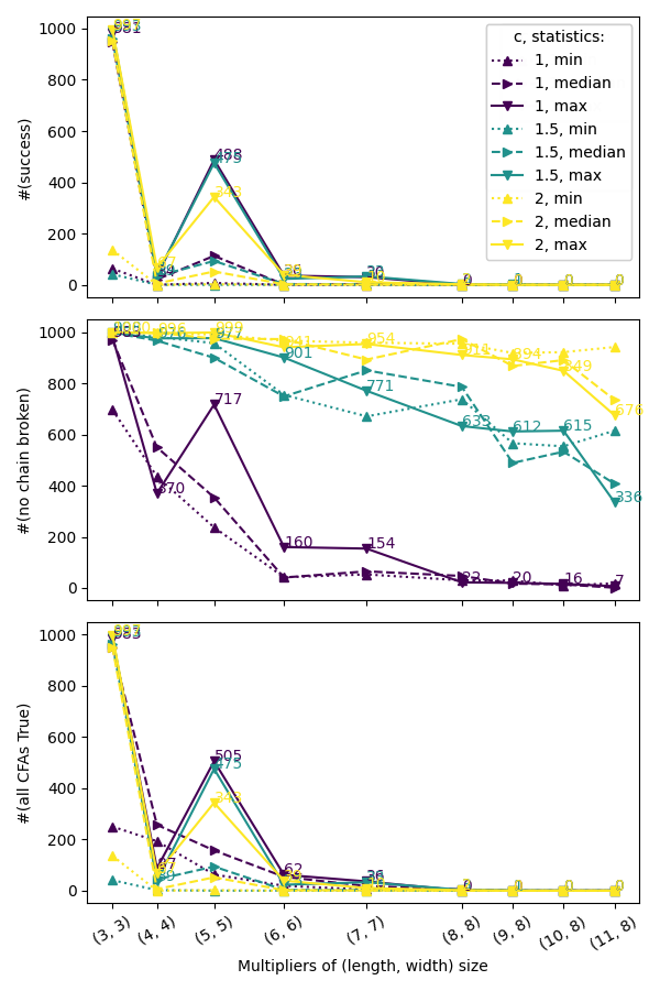
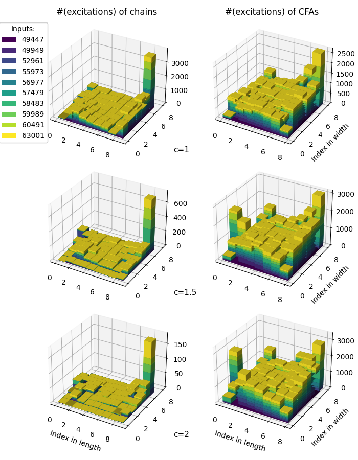
Figure 1: (Left) Comparison of different chain strengths $c,c\in\{1,1.5,2\}$, for QA to factor integers of $3+3$ bits up to $11+8$ bits, with the annealing time $T_{a}=10\mu s$ and 1,000 samples set for each problem instance.
(Right) Excitations distribution of chains (first column) and CFAs (second column) for factoring 10 integers of $8+8$ bits tested in the previous experiments, with chain strength equal to $c\in\{1,1.5,2\}$ (respectively top, middle, and bottom row).

Using the initialization approach based on CFA1 + flux biases and the same configuration of the annealing system ($T_{a}=10\mu s,1,000$ samples for each problem instance) of previous experiments, we test different chain strengths ($c\in\{1,1.5,2\}$) for QA factoring integers from $3\times 3$ up to $11\times 8$ bits, using the 10 highest co-prime number for each multiplier size.

In Figure 1 (left) we summarize the results of all samples provided the QA. Sorting them by the size of the input problem ($x$-axis), we plot respectively the number of samples successfully reaching the ground state (first plot), the number of samples having no broken chain (second plot), and the number of samples having no excited CFA (third plot). In general, we report the score of the median sample among all problems (dashed line) as a summary of the annealer behavior for each sample size. In addition, for each sample size, we provide information on the problem that reaches the ground state the least frequently (represented by the minimum dotted line in Figure 1 (left)), as well as the one that reaches the ground state the most frequently (represented by the maximum solid line in Figure 1 (left)).

We see that stronger chains ($c\in\{1.5,2\}$) do not always bring us a higher success probability in general for the chosen problem sizes, and that weaker chains ($c=1$) can produce higher success probabilities than stronger chains occasionally for middle-size problems. Notice that this result, in terms of the success probability, is consistent with what is mentioned by [10], suggesting that locally-structured embedding does not behave differently from global embedding regarding chain strengths. We also observe that as the problem size increases, weaker chains tend to be broken more easily than stronger chains. The rapidly declining dotted yellow lines confirm this phenomenon, approaching $0$ for problems of bigger size. Based on these two observations, we speculate that the strongest chain, which was chosen in [5], is the best candidate for factoring integers of up to $17\times 8$ bits, the maximal problem size they could encode into the target QA system with a locally-structured embedding.

III-C Results of incrementally fixing excited CFAs

From the experiment of the previous subsection, we can see that there seems to be a trade-off between broken chains and the excitations of CFAs: the weaker the chains are, the more likely they are broken, and the fewer the samples where the CFAs are excited. Moreover, the excitations of CFAs are not uniformly distributed. To this extent, we studied the distribution of broken chains and CFAs in 10 $8\times 8$ factoring problems, shown in Figure 1 (right). The results on excitations of chains and CFAs are reported as 3D bar plots in Figure (3rd and 4th row, respectively). Each problem instance is mapped with its color. The $x$ and the $y$ axis correspond to the column and row of the multiplier respectively; the $z$ axis represents the sum of excitations of each chain or CFA for the tested 10 problem instances. These results support testing an incremental remedy strategy based on modules.

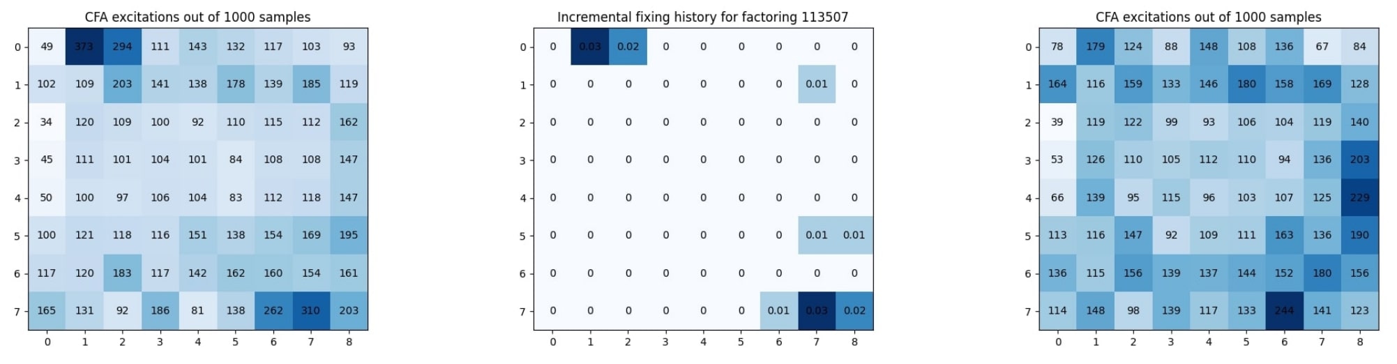
Figure 2: Fixing results for factoring 16-bit 113,507 in Table II. Each coordinate corresponds to the CFA in the multiplier circuit. The numbers in the figures in the leftmost and rightmost columns represent the number of excitations out of 1000 samples, whereas the number in the figure in the middle denotes the anneal offset used in the whole fixing process, for advancing the annealing schedule of the specific CFA. Notice the less homogeneous distribution of excitations of CFAs in the leftmost figure compared to the rightmost figure. (Left). Before the fixing. (Middle). The fixing history. (Right). After the fixing.

With the strongest chain strength and the same configuration of the annealing system as the other experiments in the paper, we test the approach of incrementally fixing excited CFAs for QA factoring the highest integers of $8\times 8$ bits up to $10\times 8$ bits from the experiments shown in Figure 1. The results are shown in Table II. To get an extensive analysis of the novel remedy strategy, we tested three different configurations, with the only difference being the number of samples obtained for each iteration (respectively 1000, 2000, and 3000). We also show in Figure 2 the behavior of the remedy strategy on one of the problem instances.

From the results, we can see that the remedy strategy helps in solving some of the problem instances. In particular, this approach works under the assumption the user has a limited amount of QPU time (i.e. the annealing time is confined to values $\lesssim 20\mu)s$, showing its effectiveness when users are bound to tight constraints in accessing the D-Wave devices. This approach works more effectively with smaller instances, reaching the ground state more frequently and with fewer iteration steps. Moreover, increasing the sample size does not impact performances, showing sporadically improvements in reaching the ground state when the number of samples increases. Nevertheless, setting the annealing offset scores based on the modules’ properties instead of targeting qubits independently seems promising, and further investigations could define different conditions to prioritize the annealing of some CFAs.

IV Discussion

This paper has built upon the recent work presented in our previous publication [5], which introduced a novel approach to the problem of PF through quantum annealing. In contrast to our previous paper, which showcased exclusively the effective techniques that highly benefited our task, here we discussed several intermediate and less successful approaches. This comprehensive exploration provides insights into the intricacies that influenced our final results in [5]. The code to replicate these experiments is reported in the following publicly available repository: https://gitlab.com/jingwen.ding/multiplier-encoder-2nd.

Our experiments revealed several insights:

• Effectiveness of Flux Biases Tuning: We showed that the techniques to initialize qubits implemented at the encoding level were not as effective as flux-biases tuning. Nevertheless, they can be considered as viable alternative to the usage of fix_variables() in other contexts.

• Chains Coupling Strength: Even though using the highest value for chains coupling strength might not be optimal for small-sized problems, it proved crucial for solving more complex problems. This highlights the delicate balance between problem size and annealing parameters, e.g. chain strength.

• Trade-off Between Broken Chains and CFA Excitations: We observed a trade-off between the presence of broken chains and the excitations of CFAs when the QA generates its samples. This further highlights the importance of monitoring chain strength in other contexts.

• Non-Uniform Distribution of CFA Excitations: The excitations of CFAs were found to be non-uniformly distributed for different samples on the same problem instance. Understanding this distribution can be valuable for tailoring annealing strategies to specific problem instances.

• Remedy Strategy for Middle-Size Problems: The remedy strategy we proposed in Section 2.4, based on the above observations, showed minor benefits in solving middle-sized problems. Nevertheless, it could be useful in other contexts.

By delving into the details of our experimental journey, listing both our successes and setbacks, we aim to provide valuable insights to a more specialized audience of D-Wave Quantum Annealer users and practitioners. Our work contributes to the evolving world of quantum annealing and equips researchers and professionals with additional knowledge to effectively use D-Wave quantum annealers in their applications.

TABLE II: Results of incrementally remedying excited CFAs for factoring integers of $8\times 8$ bits up to $10\times 8$ bits, with the same annealing time $T_{a}=10\mu s$ with the number of samples ranging from 1,000 to 3,000 set for each problem instance. For each problem, we first report the starting point sample, including its energy, the most excited CFA, and the number of its excitations respectively. Then, we report the number of iterations performed by the remedy strategy (a bold number means we did not reach the step threshold and a ground state has been found), together with the energy and the current most excited CFA.

size	#samples	1000					2000					3000
	input	$P_{F}$	(CFA, #excs)	i	$P_{F}$	(CFA, #excs)	$P_{F}$	(CFA, #excs)	i	$P_{F}$	(CFA, #excs)	$P_{F}$	(CFA, #excs)	i	$P_{F}$	(CFA, #excs)
8$\times$8	49447=251$\times$197	6.25	((6, 7), 395)	5	0.0	((0, 1), 315)	6.0	((0, 1), 1268)	32	4.083	((6, 5), 490)	4.0	((0, 1), 1377)	32	4.083	((4, 7), 894)
	49949=251$\times$199	6.083	((6, 7), 466)	4	0.0	((7, 6), 347)	4.0	((0, 1), 982)	32	4.0	((6, 5), 429)	2.0	((0, 1), 1461)	25	0.0	((5, 7), 631)
	52961=251$\times$211	2.083	((7, 5), 454)	32	6.083	((6, 7), 250)	6.167	((7, 5), 994)	32	6.167	((5, 7), 452)	6.083	((7, 5), 1705)	6	0.0	((7, 6), 1001)
	55973=251$\times$223	4.0	((5, 7), 242)	2	0.0	((7, 3), 267)	0.0	((0, 1), 569)	0	0.0	((0, 1), 569)	0.0	((7, 6), 896)	0	0.0	((7, 6), 896)
	56977=251$\times$227	2.083	((7, 6), 457)	31	0.0	((0, 1), 351)	4.083	((7, 6), 921)	8	0.0	((7, 6), 593)	4.083	((7, 6), 1555)	16	0.0	((0, 1), 739)
	57479=251$\times$229	6.0	((5, 7), 277)	32	4.0	((6, 5), 200)	4.083	((0, 1), 722)	32	4.083	((6, 6), 471)	4.0	((5, 7), 925)	1	0.0	((0, 1), 905)
	58483=251$\times$233	4.083	((7, 7), 338)	32	4.0	((0, 3), 242)	4.083	((7, 7), 779)	32	4.083	((1, 4), 452)	4.0	((7, 7), 1069)	32	4.0	((2, 1), 669)
	59989=251$\times$239	0.0	((7, 7), 252)	0	0.0	((7, 7), 252)	0.0	((7, 7), 815)	0	0.0	((7, 7), 815)	0.0	((7, 7), 1282)	0	0.0	((7, 7), 1282)
	60491=251$\times$241	2.0	((7, 7), 237)	32	4.083	((7, 7), 276)	2.0	((7, 7), 856)	32	2.0	((1, 4), 461)	2.0	((7, 7), 1082)	32	2.0	((3, 0), 589)
	63001=251$\times$251	4.083	((7, 7), 492)	4	0.0	((0, 2), 292)	2.0	((7, 7), 836)	1	0.0	((7, 7), 889)	2.0	((7, 7), 1397)	6	0.0	((7, 7), 999)
9$\times$8	100273=509$\times$197	8.167	((7, 4), 629)	34	4.083	((6, 7), 281)	8.083	((7, 4), 1413)	34	8.0	((1, 7), 490)	4.083	((7, 4), 1834)	34	4.083	((1, 7), 754)
	101291=509$\times$199	8.0	((7, 3), 461)	34	6.25	((6, 8), 288)	6.083	((7, 3), 859)	34	8.0	((6, 8), 540)	8.083	((6, 8), 1273)	34	6.083	((5, 8), 692)
	107399=509$\times$211	8.0	((7, 3), 479)	34	4.0	((7, 5), 210)	4.083	((0, 1), 1100)	34	6.083	((7, 6), 431)	6.0	((7, 3), 1485)	34	4.0	((1, 4), 701)
	113507=509$\times$223	8.0	((0, 1), 373)	13	0.0	((7, 6), 244)	4.083	((0, 1), 1133)	3	0.0	((7, 7), 995)	4.083	((0, 1), 1803)	34	6.0	((6, 7), 612)
	115543=509$\times$227	8.083	((0, 1), 541)	34	8.0	((7, 3), 214)	8.0	((0, 1), 1394)	34	6.167	((7, 6), 460)	6.0	((0, 1), 1633)	34	6.083	((0, 0), 794)
	116561=509$\times$229	6.167	((0, 1), 434)	34	8.167	((2, 5), 226)	6.0	((0, 1), 1002)	34	6.083	((6, 7), 522)	6.083	((7, 8), 1305)	34	6.083	((7, 8), 660)
	118597=509$\times$233	6.0	((0, 1), 379)	34	4.0	((2, 6), 211)	8.0	((7, 8), 880)	34	6.167	((6, 7), 363)	6.083	((7, 8), 1743)	34	6.083	((5, 8), 683)
	121651=509$\times$239	8.083	((7, 8), 628)	34	4.083	((7, 7), 274)	8.0	((7, 8), 1035)	9	0.0	((0, 2), 508)	4.0	((0, 1), 1307)	4	0.0	((0, 2), 974)
	122669=509$\times$241	6.083	((7, 8), 600)	34	4.083	((7, 6), 272)	10.0	((7, 8), 1515)	34	4.0	((0, 4), 557)	6.083	((7, 8), 2154)	34	4.0	((7, 5), 685)
	127759=509$\times$251	6.0	((0, 1), 651)	2	0.0	((0, 1), 542)	6.0	((7, 8), 1261)	2	0.0	((7, 8), 1026)	4.0	((0, 1), 1799)	2	0.0	((0, 1), 1837)
10$\times$8	201137=1021$\times$197	8.083	((7, 2), 424)	36	10.083	((7, 2), 234)	2.0	((7, 2), 881)	36	4.083	((4, 9), 463)	4.0	((7, 2), 1430)	36	6.083	((2, 9), 690)
	203179=1021$\times$199	10.083	((0, 1), 474)	36	6.083	((0, 2), 281)	8.083	((0, 1), 940)	36	6.167	((5, 7), 423)	8.083	((0, 1), 1431)	36	8.0	((7, 6), 1033)
	215431=1021$\times$211	8.0	((0, 1), 574)	36	8.0	((7, 8), 265)	6.0	((0, 1), 1033)	36	6.083	((3, 1), 422)	6.0	((0, 1), 1817)	36	8.0	((7, 3), 594)
	227683=1021$\times$223	8.083	((0, 1), 586)	36	6.167	((5, 9), 213)	4.0	((0, 1), 1318)	36	4.167	((6, 8), 419)	6.0	((0, 1), 1897)	36	4.083	((7, 4), 639)
	231767=1021$\times$227	10.0	((0, 1), 592)	36	8.083	((5, 9), 269)	8.083	((0, 1), 1146)	36	6.083	((7, 7), 452)	8.083	((0, 1), 1709)	36	6.0	((7, 6), 641)
	233809=1021$\times$229	8.083	((7, 9), 361)	36	6.167	((5, 9), 248)	6.0	((0, 1), 922)	36	8.0	((2, 9), 453)	6.167	((7, 9), 1207)	36	6.0	((7, 5), 776)
	237893=1021$\times$233	6.0	((7, 9), 456)	36	6.083	((0, 1), 185)	6.0	((7, 9), 886)	36	6.0	((1, 4), 378)	4.0	((7, 9), 1480)	36	6.0	((2, 2), 553)
	244019=1021$\times$239	8.083	((0, 1), 600)	36	4.0	((7, 9), 234)	6.167	((0, 1), 1252)	36	6.0	((1, 2), 427)	6.083	((7, 9), 1595)	30	0.0	((0, 1), 733)
	246061=1021$\times$241	2.083	((7, 9), 619)	36	6.0	((1, 1), 232)	10.0	((7, 9), 1056)	36	8.0	((1, 5), 499)	8.0	((7, 9), 1478)	36	4.0	((2, 9), 615)
	256271=1021$\times$251	4.083	((7, 9), 659)	36	4.083	((7, 8), 226)	6.083	((0, 1), 1256)	10	0.0	((0, 4), 695)	2.083	((0, 1), 1900)	36	4.083	((7, 8), 787)

References

- [1] Juan I Adame and Peter L McMahon “Inhomogeneous driving in quantum annealers can result in orders-of-magnitude improvements in performance. Quantum Science and Technology 5, 3 (jun 2020), 035011”, 2020
- [2] Mirko Amico, Zain H. Saleem and Muir Kumph “Experimental study of Shor’s factoring algorithm using the IBM Q Experience” In Phys. Rev. A 100 American Physical Society, 2019, pp. 012305 DOI: 10.1103/PhysRevA.100.012305
- [3] Evgeny Andriyash et al. “Boosting integer factoring performance via quantum annealing offsets” In D-Wave Technical Report Series 14.2016, 2016
- [4] Zhengbing Bian et al. “Solving SAT (and MaxSAT) with a quantum annealer: Foundations, encodings, and preliminary results” In Information and Computation 275, 2020, pp. 104609 DOI: https://doi.org/10.1016/j.ic.2020.104609
- [5] Jingwen Ding, Giuseppe Spallitta and Roberto Sebastiani “Effective prime factorization via quantum annealing by modular locally-structured embedding” In Scientific Reports 14.1 Nature Publishing Group UK London, 2024, pp. 3518 DOI: https://doi.org/10.1038/s41598-024-53708-7
- [6] Raouf Dridi and Hedayat Alghassi “Prime factorization using quantum annealing and computational algebraic geometry” In Scientific Reports 7.1, 2017, pp. 43048 DOI: 10.1038/srep43048
- [7] DWave. “Anneal Offsets.” https://docs.dwavesys.com/docs/latest/c_qpu_annealing.html, 2021
- [8] Shuxian Jiang et al. “Quantum Annealing for Prime Factorization” In Scientific Reports 8.1, 2018, pp. 17667 DOI: 10.1038/s41598-018-36058-z
- [9] A.H. Karamlou, W.A. Simon and A. al. Katabarwa “Analyzing the performance of variational quantum factoring on a superconducting quantum processor.” In Quantum Inf 7.156, 2021 DOI: https://doi.org/10.1038/s41534-021-00478-z
- [10] Trevor Lanting et al. “Experimental demonstration of perturbative anticrossing mitigation using nonuniform driver Hamiltonians” In Phys. Rev. A 96 American Physical Society, 2017, pp. 042322 DOI: 10.1103/PhysRevA.96.042322
- [11] Erik Lucero et al. “Computing prime factors with a Josephson phase qubit quantum processor” In Nature Physics 8.10, 2012, pp. 719–723 DOI: 10.1038/nphys2385
- [12] Enrique Martín-López et al. “Experimental realization of Shor’s quantum factoring algorithm using qubit recycling” In Nature Photonics 6.11, 2012, pp. 773–776 DOI: 10.1038/nphoton.2012.259
- [13] Riccardo Mengoni, Daniele Ottaviani and Paolino Iorio “Breaking RSA Security With A Low Noise D-Wave 2000Q Quantum Annealer: Computational Times, Limitations And Prospects”, 2020 DOI: https://doi.org/10.48550/arXiv.2005.02268
- [14] Thomas Monz et al. “Realization of a scalable Shor algorithm” In Science 351.6277, 2016, pp. 1068–1070 DOI: 10.1126/science.aad9480
- [15] Ronald L Rivest, Adi Shamir and Leonard Adleman “A method for obtaining digital signatures and public-key cryptosystems” In Communications of the ACM 21.2 ACM New York, NY, USA, 1978, pp. 120–126
- [16] Roberto Sebastiani and Patrick Trentin “OptiMathSAT: A Tool for Optimization Modulo Theories” In Journal of Automated Reasoning 64.3, 2020, pp. 423–460 DOI: 10.1007/s10817-018-09508-6
- [17] R. Selvarajan, V. Dixit and X. al. Cui “Prime factorization using quantum variational imaginary time evolution.” In Sci Rep 11.20835, 2021 DOI: https://doi.org/10.1038/s41598-021-00339-x
- [18] Lieven M.. Vandersypen et al. “Experimental realization of Shor’s quantum factoring algorithm using nuclear magnetic resonance” In Nature 414.6866, 2001, pp. 883–887 DOI: 10.1038/414883a
- [19] B. Wang, F. Hu and H. al. Yao “Prime factorization algorithm based on parameter optimization of Ising model.” In Scientific Reports 10.2020, 2020
- [20] Dennis Willsch et al. “Large-Scale Simulation of Shor’s Quantum Factoring Algorithm” In Mathematics 11.19, 2023 DOI: 10.3390/math11194222
- [21] Sheir Yarkoni et al. “Boosting quantum annealing performance using evolution strategies for annealing offsets tuning” In Quantum Technology and Optimization Problems: First International Workshop, QTOP 2019, Munich, Germany, March 18, 2019, Proceedings 1, 2019, pp. 157–168 Springer