Visibility-Aware RRT* for Safety-Critical Navigation of Perception-Limited Robots in Unknown Environments

Abstract

Safe autonomous navigation in unknown environments remains a critical challenge for robots with limited sensing capabilities. While safety-critical control techniques, such as Control Barrier Functions (CBFs), have been proposed to ensure safety, their effectiveness relies on the assumption that the robot has complete knowledge of its surroundings. In reality, robots often operate with restricted field-of-view and finite sensing range, which can lead to collisions with unknown obstacles if the planning algorithm is agnostic to these limitations. To address this issue, we introduce the visibility-aware RRT* algorithm that combines sampling-based planning with CBFs to generate safe and efficient global reference paths in partially unknown environments. The algorithm incorporates a collision avoidance CBF and a novel visibility CBF, which guarantees that the robot remains within locally collision-free regions, enabling timely detection and avoidance of unknown obstacles. We conduct extensive experiments interfacing the path planners with two different safety-critical controllers, wherein our method outperforms all other compared baselines across both safety and efficiency aspects.

I INTRODUCTION

Autonomous navigation in unknown environments is a fundamental challenge in robotics, with applications ranging from exploration and search-and-rescue to autonomous driving. A general navigation stack comprises four key components: localization, mapping, planning, and control. Localization and mapping enable robots to build a map of their surroundings using onboard sensors, such as Visual Simultaneous Localization and Mapping (VSLAM) systems. However, these sensors often have limitations, including restricted field-of-view (FOV) and finite sensing range. For instance, popular off-the-shelf RGB-D cameras’ horizontal FOV are often less than 70^∘ [1].

To ensure safe navigation, there has been growing interest in safety-critical controllers, such as those based on Control Barrier Functions (CBFs) [2], which enforce safety objectives on controlled systems. These controllers theoretically guarantee safety by keeping the robot within a safe set, assuming that nearby obstacles are fully known a priori. However, in practice, the effectiveness of these controllers relies heavily on the robot’s ability to perceive potential obstacles in the local environment. If the global planner does not account for the robot’s limited sensing capabilities under the presence of unknown obstacles, the theoretical safety guarantees may not hold, leading to potentially hazardous situations.

Several approaches have been proposed to improve the safety of navigation under sensing limitations. Some methods use nonlinear optimization to generate [3] or refine [4] perception-aware paths, but these approaches can be computationally intensive and the solution convergence is not guaranteed. Other approaches first plan a path and then optimize the heading angle to enhance safety based on sensing objectives [5, 6, 7], although they do not always guarantee safety. Another method computes local safe regions during the exploration of candidate paths to account for local sensing information and ensure safety [8], but it requires storing all combinations of such regions, making the planning module overly computationally expensive.

In this paper, we propose a visibility-aware RRT* algorithm that explicitly reasons about the robot’s limited sensing capabilities and combines the benefits of sampling-based planning with CBFs to enable safe and efficient navigation in partially unknown environments. Our approach incorporates two types of CBFs: (i) a collision avoidance CBF to ensure that the planned path is collision-free with respect to known obstacles, and (ii) a novel visibility CBF, which we introduce in this work, that guarantees the local tracking controller following the resulting path will always keep the robot within locally collision-free regions. This ensures that the robot can detect unknown obstacles in a timely manner, enabling the robot to avoid them by virtue of the local controller. We demonstrate the effectiveness of our method through extensive simulations and comparisons with other planning methods. The results indicate that our method can be seamlessly incorporated with safety-critical controllers, outperforming existing baselines in both safety and efficiency metrics across multiple scenarios.

II PRELIMINARIES

II-1 System Description

We consider a robot that is modeled as a continuous-time, control-affine system:

$$\dot{{\bm{x}}}=F({\bm{x}},{\bm{u}})=f({\bm{x}})+g({\bm{x}}){\bm{u}},$$ (1)

where ${\bm{x}}\in\mathcal{X}\subset\mathbb{R}^{n}$ is the state, and ${\bm{u}}\in\mathcal{U}\subset\mathbb{R}^{m}$ is the control input, with $\mathcal{U}$ being a set of admissible controls for System (1). The functions $f:\mathcal{X}\to\mathbb{R}^{n}$ and $g:\mathcal{U}\to\mathbb{R}^{n\times m}$ are assumed to be locally Lipschitz continuous.

We assume the robot has limited sensing capabilities, modeled via a field-of-view angle $\theta_{\text{fov}}<360^{\circ}$ and a maximum sensing range $l_{\text{range}}<\infty$ of the onboard sensor.

II-2 Linear Quadratic Regulator

Linear Quadratic Regulator (LQR) computes optimal control policies for linear systems, and can be applied to nonlinear systems by linearizing the system around an operating point $({\bm{x}}_{o},{\bm{u}}_{o})$, i.e., taking the first-order Taylor expansion of a nonlinear dynamics $F$ around this point:

$$\dot{{\bm{x}}}\approx F({\bm{x}}_{o},{\bm{u}}_{o})+A\bar{{\bm{x}}}+B\bar{{\bm{u}}},$$ (2)

where $\bar{{\bm{x}}}={\bm{x}}-{\bm{x}}_{o}$, $\bar{{\bm{u}}}={\bm{u}}-{\bm{u}}_{o}$, $A=\frac{\partial F}{\partial{\bm{x}}}|_{({\bm{x}}_{o},{\bm{u}}_{o})}$, $B=\frac{\partial F}{\partial{\bm{u}}}|_{({\bm{x}}_{o},{\bm{u}}_{o})}$. Given an infinite time horizon cost function:

$$J=\int_{0}^{\infty}(\,\bar{{\bm{x}}}^{\top}Q\bar{{\bm{x}}}+\bar{{\bm{u}}}^{\top}R\bar{{\bm{u}}}\,)\,\mathrm{d}t,$$ (3)

where $Q=Q^{\top}\succeq 0$ and $R=R^{\top}\succ 0$ are weight matrices, one can compute the locally optimal control policy $\mathcal{K}_{\text{lqr}}^{*}({\bm{x}})=-K_{\text{lqr}}{\bm{x}}$ by solving the algebraic Riccati equation:

$$A^{\top}P+PA-PBR^{-1}B^{\top}P+Q=0.$$ (4)

Solving (4) for $P$, the LQR gain matrix is:

$$K_{\text{lqr}}=R^{-1}B^{\top}P.$$ (5)

II-3 Control Barrier Functions

Definition 1 (Control Barrier Function (CBF)).

Let $\mathcal{C}=\{{\bm{x}}\in\mathcal{X}:h({\bm{x}})\geq 0\}$, where $h:\mathcal{X}\rightarrow\mathbb{R}$ is a continuously differentiable function. The function $h$ is a CBF on $\mathcal{C}$ for System (1) if there exists a class $\mathcal{K}$ function $\alpha$ such that

$$\sup_{{\bm{u}}\in\mathcal{U}}\left[L_{f}h({\bm{x}})+L_{g}h({\bm{x}}){\bm{u}}\right]\geq-\alpha(h({\bm{x}})),$$ (6)

for all ${\bm{x}}\in\mathcal{X}$ and $L_{f}h({\bm{x}})$ and $L_{g}h({\bm{x}})$ denote the Lie derivatives of $h$ along $f$ and $g$, respectively [9].

Theorem 1.

Given a CBF $h$ with the associated set $\mathcal{C}$, any Lipschitz continuous controller ${\bm{u}}\in\mathcal{K}_{\textup{cbf}}({\bm{x}})$, with $\mathcal{K}_{\textup{cbf}}({\bm{x}})=\{{\bm{u}}\in\mathcal{U}:L_{f}h({\bm{x}})+L_{g}h({\bm{x}}){\bm{u}}+\alpha(h({\bm{x}}))\geq 0\}$, renders $\mathcal{C}$ forward invariant for System (1). See [9].

II-4 High Order CBF

The concept of CBFs has been extended to High Order CBFs (HOCBFs) [10], which provide a more general formulation that can be used for constraints of high relative degree. In this work, we focus on time-invariant HOCBFs, which generalize the concept of exponential CBFs proposed in [11].

For a $r_{b}^{\textup{th}}$ order differentiable function $h:\mathcal{X}\rightarrow\mathbb{R}$, we define a series of functions $\psi_{i}:\mathcal{X}\rightarrow\mathbb{R}$, $i=0,\ldots,r_{b}$, as:

$$\psi_{0}({\bm{x}}) :=h({\bm{x}}),$$ (7a)

$$\psi_{1}({\bm{x}}) :=\dot{\psi}_{0}({\bm{x}})+\alpha_{1}(\psi_{0}({\bm{x}})),$$ (7b)

$$\vdots$$

$$\psi_{r_{b}}({\bm{x}}) :=\dot{\psi}_{r_{b}-1}({\bm{x}})+\alpha_{r_{b}}(\psi_{r_{b}-1}({\bm{x}})),$$ (7c)

where $\alpha_{i}:\mathbb{R}^{+}\rightarrow\mathbb{R}^{+}$, $i=1,\ldots,r_{b}$, denote class $\mathcal{K}$ functions, and $\dot{\psi}_{i}({\bm{x}})=L_{f}\psi_{i}({\bm{x}})+L_{g}\psi_{i}({\bm{x}}){\bm{u}}$. We further define a series of sets $\mathcal{C}_{i}$ associated with these functions as:

$$\mathcal{C}_{1} :=\{{\bm{x}}\in\mathcal{X}:\psi_{0}({\bm{x}})\geq 0\},$$ (8a)

$$\mathcal{C}_{2} :=\{{\bm{x}}\in\mathcal{X}:\psi_{1}({\bm{x}})\geq 0\},$$ (8b)

$$\vdots$$

$$\mathcal{C}_{r_{b}} :=\{{\bm{x}}\in\mathcal{X}:\psi_{r_{b}-1}({\bm{x}})\geq 0\}.$$ (8c)

Definition 2 (HOCBF).

The function $h:\mathcal{X}\rightarrow\mathbb{R}$ is a HOCBF of relative degree $r_{b}$ for System (1) if there exist differentiable class $\mathcal{K}$ functions $\alpha_{1},\alpha_{2},\ldots,\alpha_{r_{b}}$ such that

$$\psi_{r_{b}}({\bm{x}})\geq 0,\quad\forall{\bm{x}}\in\mathcal{C}_{1}\cap\mathcal{C}_{2}\cap\ldots\cap\mathcal{C}_{r_{b}}.$$ (9)

Theorem 2.

Given a HOCBF $h$ with the associated sets $\mathcal{C}_{1},\mathcal{C}_{2},\ldots,\mathcal{C}_{r_{b}}$, if ${\bm{x}}(t_{0})\in\mathcal{C}_{1}\cap\mathcal{C}_{2}\cap\ldots\cap\mathcal{C}_{r_{b}}$, then any Lipschitz continuous controller ${\bm{u}}(t)\in\mathcal{K}_{\textup{hocbf}}({\bm{x}})$, with $\mathcal{K}_{\textup{hocbf}}({\bm{x}})=\{{\bm{u}}\in\mathcal{U}:\psi_{r_{b}}({\bm{x}})\geq 0\}$, renders the set $\mathcal{C}_{1}\cap\mathcal{C}_{2}\cap\ldots\cap\mathcal{C}_{r_{b}}$ forward invariant for system (1) [10].

III PROBLEM FORMULATION

Consider a robot modeled as the nonlinear system (1) navigating in an unknown environment $\mathcal{W}$. The environment $\mathcal{W}$ consists of two types of obstacles: a set $\mathcal{O}_{0}\subset\mathcal{W}$ of known obstacles at the initial time $t_{0}$, and a set $\mathcal{H}\subset\mathcal{W}$ of unknown (or “hidden”) obstacles that can be sensed by the robot on-the-fly as it navigates through the environment. The true obstacle-free space $\mathcal{S}$ is then defined as $\mathcal{S}=\mathcal{W}\setminus(\mathcal{O}_{0}\cup\mathcal{H})$. A local tracking control policy $\pi:[t_{0},\infty)\times\mathcal{X}\times\mathcal{X}\to\mathcal{U}$ takes the current time $t$, the current state ${\bm{x}}_{t}:=\bm{x}(t)$, and a reference state ${\bm{x}}_{t}^{\textup{ref}}\in\mathcal{X}$ as inputs, and generates as outputs the control inputs that track a nominal path from the current to reference state. Given the initial condition ${\bm{x}}(t_{0})={\bm{x}}_{0}$, $t\geq t_{0}$, the robot dynamics obey:

$$\dot{{\bm{x}}}(t)=f({\bm{x}}(t))+g({\bm{x}}(t))\pi(t,{\bm{x}}_{t},{\bm{x}}_{t}^{\textup{ref}}),\quad{\bm{x}}(t_{0})={\bm{x}}_{0}.$$ (10)

The navigation problem is divided into two hierarchical steps: 1) finding a global reference path $p^{\textup{ref}}$, and 2) tracking $p^{\textup{ref}}$ using a local controller.

Global Path Planning: Given a goal state ${\bm{x}}_{\textup{goal}}\in\mathcal{X}$, the objective of the global path planner is to find a global reference path $p^{\textup{ref}}:\mathcal{X}\to\mathcal{P}$, represented by a set of waypoints $\mathcal{P}=\{{\bm{x}}_{i}^{\textup{ref}}\in\mathcal{X}\}_{i=0}^{N}$, where ${\bm{x}}_{0}^{\textup{ref}}={\bm{x}}_{0}$ and ${\bm{x}}_{N}^{\textup{ref}}={\bm{x}}_{\textup{goal}}$ are the initial and final waypoints in $\mathcal{P}$, respectively. For any given state ${\bm{x}}_{t}$, the function yields the next waypoint that the robot should navigate towards as:

$${\bm{x}}_{i}^{\textup{ref}}=p^{\textup{ref}}({\bm{x}}_{t}),$$ (11)

where ${\bm{x}}_{i}^{\textup{ref}}\in\mathcal{P}\subset\mathcal{X}$ indicates the immediate waypoint for navigation. The reference path should satisfy:

$$p^{\textup{ref}}({\bm{x}}_{t})\in\mathcal{S},\quad\forall t\geq t_{0},\quad\forall{\bm{x}}_{t}\in\mathcal{X}.$$ (12)

However, the true collision-free set $\mathcal{S}$ is often unknown in advance.

Definition 3 (Collision-Free Path).

We define the known collision-free set at $t_{0}$ as $\mathcal{S}_{0}=\mathcal{W}\setminus\mathcal{O}_{0}$. A reference path $p^{\textup{ref}}$ is considered collision-free if it satisfies the condition:

$$p^{\textup{ref}}({\bm{x}}_{t})\in\mathcal{S}_{0},\quad\forall t\geq t_{0},\quad\forall{\bm{x}}_{t}\in\mathcal{X}.$$ (13)

Let ${\bm{r}}_{t}=[x_{t},y_{t}]^{\top}\in\mathbb{R}^{2}$ and $\theta_{t}\in\mathbb{R}$ denote the position and orientation of the robot with respect to a global frame at time $t$, respectively. The sensing footprint $\mathcal{F}_{t}$, which represents the currently sensed area at time $t$, is defined as:

$$\mathcal{F}_{t}=\bigg{\{}{\bm{p}}\in\mathcal{S}\mid \,\|{\bm{p}}-{\bm{r}}_{t}\|\leq l_{\textup{range}}$$

$$\cap\,|\,\angle({\bm{p}}-{\bm{r}}_{t},\theta_{t})\,|\leq\frac{\theta_{\textup{fov}}}{2}\bigg{\}},$$ (14)

where $\|{\bm{p}}-{\bm{r}}_{t}\|$ represents the Euclidean distance between a point ${\bm{p}}\in\mathcal{W}$ and the robot’s position ${\bm{r}}_{t}$, $\angle({\bm{p}}-{\bm{r}}_{t},\theta_{t})$ denotes the angle between the vector ${\bm{p}}-{\bm{r}}_{t}$ and the robot’s orientation $\theta_{t}$. Given the accumulated sensory information collected from time $t_{0}$ to $t$, we define the known collision-free space $\mathcal{B}_{t}$ at time $t$ as:

$$\mathcal{B}_{t}:=\bigcup_{\tau=t_{0}}^{t}\mathcal{F}_{\tau}\subseteq\mathcal{S}.$$ (15)

Consequently, the part of the environment that has not been sensed yet is $\mathcal{S}\setminus\mathcal{B}_{t}$, and is called the unmeasured space at time $t$.

It is important to note that the collision-free path criterion (13) treats all unmeasured space $\mathcal{S}\setminus\mathcal{B}_{t_{0}}$ at time $t_{0}$ as free space. However, while following the path $p^{\textup{ref}}$ using the local controller $\pi$ after the planning cycle, unknown obstacles $\mathcal{H}$ might exist within such unmeasured spaces.

Given this context, we introduce a stronger criterion that underlines the path’s visibility and safety by requiring the robot to stay within the known local collision-free space $\mathcal{B}_{t}$, thereby mitigating the risk posed by unknown obstacles [8].

Definition 4 (Visibility-Aware Path).

A reference path $p^{\textup{ref}}$ is called visibility-aware w.r.t. the dynamics (1) if the updated state ${\bm{x}}(t+\Delta t)$, for a small time increment $\Delta t>0$, under the local tracking controller $\pi(t,{\bm{x}}_{t},p^{\textup{ref}}({\bm{x}}_{t}))$ satisfies:

$${\bm{x}}(t+\Delta t)\in\mathcal{B}_{t},\quad\forall t\geq t_{0},\quad\forall{\bm{x}}_{t}\in\mathcal{X}.$$ (16)

In the following sections, we present the construction of a global path planner that imposes (16) (see Sec. IV), and demonstrate how (16) ensures hidden obstacles are avoidable, in the sense that the local tracking controller is able to generate collision-free trajectories (see Sec. V).

Local Tracking Control: A local control policy $\pi$ is used to stabilize the systems around the subsequent waypoint ${\bm{x}}_{i}^{\textup{ref}}$ (11) and to ensure that the robot remains within the true collision-free set $\mathcal{S}$. The local controller is assumed to be capable of tracking the path between subsequent waypoints with a tracking error bounded by a maximum displacement $\epsilon$. As $p^{\textup{ref}}$ continuously updates the waypoint, it drives the robot towards the goal state ${\bm{x}}_{\textup{goal}}$. There exists a plethora of methodologies to design such controllers [9, 12]. Since the primary focus of this paper is on designing a visibility-aware path planner, we will discuss two case studies of such controllers in Sec. V and Sec. VI to highlight the advantages of our proposed planner when utilized alongside various local controllers.

IV GLOBAL PATH PLANNER

In this section, we introduce the Visibility-Aware RRT* algorithm, which aims to solve the motion planning problem under limited sensing capabilities while satisfying the visibility condition given in (16). The proposed algorithm builds upon the LQR-RRT* framework [13] by incorporating two CBFs that guide the search process to ensure satisfaction of both the collision-free (13) and visibility-aware (16) properties.

IV-A Visibility-Aware RRT*

Initialization: $\mathcal{V}\leftarrow$ $\{{\bm{x}}_{0}\}$; $\mathcal{E}\leftarrow\emptyset$;

for $i=1,\ldots,\texttt{{maxIter}}$ do

       ${\bm{x}}_{\textup{rand}}\leftarrow\texttt{Sample}()$;

       ${\bm{x}}_{\textup{nearest}}\leftarrow\texttt{Nearest}(\mathcal{V},{\bm{x}}_{\textup{rand}})$;

       ${\bm{x}}_{\textup{rand}}\leftarrow\texttt{SetAngle}({\bm{x}}_{\textup{rand}},{\bm{x}}_{\textup{nearest}})$;

       ${\bm{x}}_{\textup{new}},\_\leftarrow\texttt{LQR-CBF-Steer}({\bm{x}}_{\textup{nearest}},{\bm{x}}_{\textup{rand}})$;

       $\mathcal{X}_{\textup{near}}\leftarrow\texttt{NearbyNode}(\mathcal{V},{\bm{x}}_{\textup{new}})$;

       ${\bm{x}}_{\textup{min}}\leftarrow\texttt{ChooseParent}(\mathcal{X}_{\textup{near}},{\bm{x}}_{\textup{new}})$;

       if ${\bm{x}}_{\textup{min}}\neq\texttt{{None}}$ then

             $\mathcal{V}\leftarrow\mathcal{V}\cup\{{\bm{x}}_{\textup{new}}\}$;

             $\mathcal{E}\leftarrow\mathcal{E}\cup\{({\bm{x}}_{\textup{min}},{\bm{x}}_{\textup{new}})\}$;

             $\texttt{Rewire}(\mathcal{X}_{\textup{near}},{\bm{x}}_{\textup{new}})$;

            

      

$\mathcal{P}\leftarrow\texttt{ExtractPath}(\mathcal{V},{\bm{x}}_{\textup{0}},{\bm{x}}_{\textup{goal}})$;

return $\mathcal{P}$;

Algorithm 1 Visibility-Aware RRT*

The LQR-RRT* [13] is a sampling-based motion planning algorithm that incorporates the LQR controller as a steering function for nonlinear systems with non-holonomic constraints. It guarantees probabilistic completeness and inherits the asymptotic optimality property from the RRT* algorithm through its rewiring process [14]. Recently, Yang et al. [15] proposed an extension to the LQR-RRT* that incorporates CBF constraints during the planning process. Instead of formulating and solving Quadratic Programs (QPs) iteratively, as done in existing works [16], it checks whether the CBF constraints are satisfied and uses them as the termination condition for the steering process.

In our work, we modify the LQR-RRT* baseline to include the robot’s orientation angle $\theta$ at each node, in addition to the position coordinates $(x,y)$. This modification allows it to consider the robot’s rotational motion and field of view during the planning process, essential for accommodating the robot’s sensing limitations.

The overall algorithm, as shown in Alg. 1, iteratively expands a tree $(\mathcal{V},\mathcal{E})$ in the configuration space $\mathcal{W}$ until a maximum number of iterations (denoted as maxIter) is reached. The components of the algorithm are as follows:

• Sample: Randomly samples a state ${\bm{x}}_{\text{rand}}=[x_{\text{rand}},y_{\text{rand}},\theta_{\text{rand}}]^{\top}$ within the configuration space to expand the tree towards.

• Nearest: Finds the nearest node ${\bm{x}}_{\text{nearest}}$ in the current vertices in the tree $\mathcal{V}$ to the sampled state ${\bm{x}}_{\text{rand}}$.

• SetAngle: Assigns the orientation angle $\theta_{\text{rand}}$ to the sampled state ${\bm{x}}_{\text{rand}}$ based on the direction from the nearest node ${\bm{x}}_{\text{nearest}}$ to ${\bm{x}}_{\text{rand}}$: $\theta_{\text{rand}}=\arctan\left(\frac{y_{\text{rand}}-y_{\text{nearest}}}{x_{\text{rand}}-x_{\text{nearest}}}\right)$.

• LQR-CBF-Steer: Generates a new node ${\bm{x}}_{\text{new}}$ by steering from ${\bm{x}}_{\text{nearest}}$ towards ${\bm{x}}_{\text{rand}}$. The details are described below.

• NearbyNode: Identifies a set of nearby nodes $\mathcal{X}_{\text{near}}$ within a pre-defined euclidean distance from ${\bm{x}}_{\text{new}}$.

• ChooseParent: Selects the best parent node ${\bm{x}}_{\text{min}}$ for the new node ${\bm{x}}_{\text{new}}$ from the set of nearby nodes $\mathcal{X}_{\text{near}}$ based on the cost and the feasibility of the connecting trajectory generated by the steering function. Given a trajectory $\bm{\sigma}=({\bm{x}}(t),{\bm{u}}(t))$, where $t\in[0,T]$ and $T$ is the duration of the trajectory, the evaluated cost is defined as:

  $$\texttt{cost}(\bm{\sigma})=\int_{0}^{T}\left({\bm{x}}(t)^{\top}Q{\bm{x}}(t)+{\bm{u}}(t)^{\top}R{\bm{u}}(t)\right)\,\mathrm{d}t,$$ (17)

  where the $Q$ and $R$ are the same weight matrices as in (3) (see Alg. 2).

• Rewire: Performs the rewiring process by considering the new node ${\bm{x}}_{\text{new}}$ as a potential parent for the nearby nodes in $\mathcal{X}_{\text{near}}$. If a trajectory from ${\bm{x}}_{\text{new}}$ to any nearby node ${\bm{x}}_{\text{near}}\in\mathcal{X}_{\text{near}}$ is found with a smaller cost (17), the tree is optimized by rewiring ${\bm{x}}_{\text{near}}$ to ${\bm{x}}_{\text{new}}$ (see Alg. 3).

• ExtractPath: Searches for a path from ${\bm{x}}_{\text{goal}}$ to ${\bm{x}}_{\text{start}}$ within the tree $(\mathcal{V},\mathcal{E})$. If a feasible path is found, it returns the solution path as a set of waypoints $\mathcal{P}$.

minCost $\leftarrow\infty$; ${\bm{x}}_{\textup{min}}\leftarrow\texttt{{None}}$;

for ${\bm{x}}_{\textup{near}}\in\mathcal{X}_{\textup{near}}$ do

       $\_,\bm{\sigma}\leftarrow\texttt{LQR-CBF-Steer}({\bm{x}}_{\textup{near}},{\bm{x}}_{\textup{new}})$;

       if $\bm{\sigma}\neq\texttt{{None}}$ then

             if ${\bm{x}}_{\textup{near}}.\texttt{{cost}}+\texttt{{Cost}}(\bm{\sigma})<\texttt{{minCost}}$ then

                   minCost $\leftarrow{\bm{x}}_{\textup{near}}.\texttt{cost}+\texttt{Cost}(\bm{\sigma})$;

                   ${\bm{x}}_{\textup{min}}\leftarrow{\bm{x}}_{\textup{near}}$;

                  

            

      

${\bm{x}}_{\text{new}}.\texttt{parent}\leftarrow{\bm{x}}_{\text{min}}$;

${\bm{x}}_{\text{new}}.\texttt{cost}\leftarrow\texttt{minCost}$;

return ${\bm{x}}_{\textup{min}}$;

Algorithm 2 ChooseParent($\mathcal{X}_{\textup{near}}$, ${\bm{x}}_{\textup{new}}$)

for ${\bm{x}}_{\textup{near}}\in\mathcal{X}_{\textup{near}}$ do

       $\_,\bm{\sigma}\leftarrow\texttt{LQR-CBF-Steer}({\bm{x}}_{\textup{new}},{\bm{x}}_{\textup{near}})$;

       if $\bm{\sigma}\neq\texttt{{None}}$ then

             if ${\bm{x}}_{\textup{new}}.\texttt{{cost}}+\texttt{{Cost}}(\bm{\sigma})<{\bm{x}}_{\textup{near}}.\texttt{{cost}}$ then

                   ${\bm{x}}_{\textup{near}}.\texttt{parent}\leftarrow{\bm{x}}_{\textup{new}}$;

                   ${\bm{x}}_{\textup{new}}.\texttt{cost}\leftarrow\texttt{{Cost}}(\bm{\sigma})$;

                  

            

      

Algorithm 3 Rewire($\mathcal{X}_{\textup{near}}$, ${\bm{x}}_{\textup{new}}$)

$\mathcal{X}^{\prime}\leftarrow[{\bm{x}}_{\textup{start}}]$; $\mathcal{U}^{\prime}\leftarrow[]$; ${\bm{x}}^{\prime}_{0}\leftarrow{\bm{x}}_{\textup{start}}$;

$K_{\textup{lqr}}\leftarrow\texttt{LQRsolver}({\bm{x}}_{\textup{next}})$

for $t=1,\ldots,T$ do

       ${\bm{x}}^{\prime}_{t},{\bm{u}}^{\prime}_{t}\leftarrow\texttt{Integrator}({\bm{x}}^{\prime}_{t-1},K_{\textup{lqr}})$;

       if  $\forall\,\texttt{{CBFConstraint}}({\bm{x}}^{\prime}_{t},{\bm{u}}^{\prime}_{t})$ are satisfied then

             $\mathcal{X}^{\prime}.\texttt{append}({\bm{x}}^{\prime}_{t})$; $\mathcal{U}^{\prime}.\texttt{append}({\bm{u}}^{\prime}_{t})$;

            

      else

             break;

      

${\bm{x}}_{\textup{new}}\leftarrow{\bm{x}}^{\prime}_{t}$;

return ${\bm{x}}_{\textup{new}},\bm{\sigma}=(\mathcal{X}^{\prime},\mathcal{U}^{\prime})$;

Algorithm 4 LQR-CBF-Steer(${\bm{x}}_{\textup{start}},{\bm{x}}_{\textup{next}}$)

The LQR-CBF-Steer is the key function that allows the algorithm to use LQR (5) and CBF (6) as an extension heuristic between two nodes ${\bm{x}}_{\text{start}}$ and ${\bm{x}}_{\text{next}}$ (see Alg. 4). It first linearizes the dynamics around ${\bm{x}}_{\text{next}}$ (2) and computes the optimal gain $K_{\text{lqr}}$ using the Riccatti equation (5). The function then employs the LQR controller $\mathcal{K}_{\text{lqr}}^{*}$ to generate a sequence of intermediate states $\mathcal{X}^{\prime}=\{{\bm{x}}_{\text{start}},{\bm{x}}^{\prime}_{1},\ldots,{\bm{x}}^{\prime}_{T}\}$ and control inputs $\mathcal{U}^{\prime}=\{{\bm{u}}^{\prime}_{1},\ldots,{\bm{u}}^{\prime}_{T}\}$, steering the state from ${\bm{x}}_{\text{start}}$ towards ${\bm{x}}_{\text{next}}$ based on the linearized dynamics. Throughout this process, it verifies that all CBF constraints are satisfied for each state-action pair $({\bm{x}}^{\prime}_{t},{\bm{u}}^{\prime}_{t})$ at each discretized time step $t$. If any constraint is violated, the steering extension is immediately terminated [15].

One of the main advantages of this method is its efficiency in handling multiple CBF constraints. By avoiding the need to solve QPs iteratively, the algorithm significantly reduces computational overhead, and also circumvents the issue of recursive feasibility that arises from the parameters of CBF and QP [17]. In the following sections, we introduce two types of CBFs to ensure that the resulting path is both collision-free (13) and visibility-aware (16).

IV-B HOCBF for Collision Avoidance

In this work, we employ the unicycle model to demonstrate the proposed algorithm; however, the algorithm can be derived in the same way for more complex system dynamics that include rotational motion. The unicycle model is as follows:

$$\dot{{\bm{x}}} =\begin{bmatrix}\cos\theta&0\\ \sin\theta&0\\ 0&1\end{bmatrix}\begin{bmatrix}v\\ \omega\end{bmatrix}=g({\bm{x}}){\bm{u}},$$ (18)

where ${\bm{x}}=[x,y,\theta]^{\top}\in\mathcal{X}$ is the state vector and the control input ${\bm{u}}=[v,\omega]^{\top}\in\mathcal{U}$ represents the translational velocity $v$ and angular velocity $\omega$.

Hereafter, we abuse the notation and use ${\bm{x}}_{t}$ and ${\bm{u}}_{t}$ to refer to ${\bm{x}}^{\prime}_{t}$ and ${\bm{u}}^{\prime}_{t}$ in the context of the LQR-CBF-Steer function (Alg. 4). Let one of the obstacles with radius $r_{\text{obs}}\in\mathbb{R}^{+}$ be located at $(x_{\text{obs}},y_{\text{obs}})\in\mathbb{R}^{2}$. The constraint function (7a) for collision avoidance, considering the robot radius $r_{\text{r}}$ and the maximum tracking error $\epsilon$ mentioned in Sec. III, is defined as:

$$h_{\textup{col}}({\bm{x}}_{t})=(x_{t}-x_{\text{obs}})^{2}+(y_{t}-y_{\text{obs}})^{2}-(r_{\text{obs}}+r_{\text{r}}+\epsilon)^{2}.$$ (19)

Given the dynamics (18), the function $h_{\textup{col}}({\bm{x}}_{t})$ (19) has relative degree $r_{b}=1$ for the control input $v$ and $r_{b}=2$ for the control input $\omega$. To simplify the construction of the CBF constraint, we fix the translational velocity $v$ to a constant value and only control the angular velocity $\omega$ [16].

Then, the HOCBF constraint (9) with $r_{b}=2$ is [16]:

$$\psi_{\textup{col}}({\bm{x}}_{t}) =2(x_{t}-x_{\text{obs}})v^{2}\cos^{2}{\theta_{t}}+2(y_{t}-y_{\text{obs}})v^{2}\sin^{2}{\theta_{t}}$$

$$+[2(y_{t}-y_{\text{obs}})v\cos{\theta_{t}}-2(x_{t}-x_{\text{obs}})v\sin{\theta_{t}}]\omega_{t}$$

$$+k_{1}L_{f}h_{\textup{col}}({\bm{x}}_{t})+k_{2}h_{\textup{col}}({\bm{x}}_{t})\geq 0,$$ (20)

where $k_{1}$ and $k_{2}$ are positive constants that are designed to satisfy the HOCBF condition (9), and

$$L_{f}h_{\textup{col}}({\bm{x}}_{t})=2v(x_{t}-x_{\text{obs}})\cos{\theta_{t}}+2v(y_{t}-y_{\text{obs}})\sin{\theta_{t}}.$$ (21)

Constraint (20) is then incorporated into the LQR-CBF-Steer function, ensuring that every node added to the tree is collision-free, as illustrated in Fig. 1a.

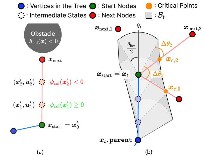
Figure 1: Illustration of the CBF constraints in the LQR-CBF-Steer function. The Integrator generates a sequence of intermediate states using the LQR gain $K_{\text{lqr}}$. At each intermediate state, the CBFConstraints are checked to ensure that the state satisfies the given constraints. If any constraint is violated, the steering process is terminated, and the last satisfied state is returned as the new node. (a) An example demonstrating the collision avoidance HOCBF constraint (20). (b) An example demonstrating the visibility CBF constraint (28). ${\bm{x}}_{\text{next},1}$ is already within the FOV at ${\bm{x}}_{t}$, satisfying the visibility constraint. For ${\bm{x}}_{\text{next},2}$, although it is outside the current FOV, it satisfies the visibility constraint. ${\bm{x}}_{\text{next},3}$ might satisfy the visibility constraint $h_{\text{vis}}({\bm{x}}_{t})\geq 0$ (27), but it violates the visibility CBF constraint $\psi_{\textup{vis}}({\bm{x}}_{t})\geq 0$ (28), causing the steering to terminate.

IV-C Incorporating Visibility Constraint into CBF

The collision-free path planning discussed in Section IV-B assumes the environment is fully known, i.e., $\mathcal{S}_{0}=\mathcal{S}$. However, partially-known environments and limited perception, such as restricted FOV and sensing range, can pose significant challenges in ensuring safe navigation. To mitigate the risks posed by these limitations, we introduce a visibility constraint formulated as a CBF to ensure that the generated path allows for any newly-detected obstacles to be avoided by a local tracking controller.

Definition 5 (Critical Point).

A critical point, denoted as ${\bm{x}}_{c}=[x_{c},y_{c},\theta_{c}]^{\top}$, is the intersecting point between the frontier $\partial\mathcal{B}_{t}$, which represents the boundary of the explored collision-free space $\mathcal{B}_{t}$ up to the current time $t$, and the path from the start node ${\bm{x}}_{t}$ to the next node ${\bm{x}}_{\textup{next}}$. The angle $\theta_{c}$ represents the direction from ${\bm{x}}_{t}$ to ${\bm{x}}_{c}$.

The critical point ${\bm{x}}_{c}$ represents the last sensed point along the linearized path (as illustrated in Fig. 1b), beyond which the robot has no updated information about potential unknown obstacles. The goal is to enforce the robot to have seen the critical point within its FOV before reaching it. To achieve this, we formulate a visibility constraint based on the time required for the robot to rotate towards and observe the critical point, denoted as $t_{\text{rot}}(\theta_{t})$, and the time needed to reach it, denoted as $t_{\text{reach}}(x_{t},y_{t})$. The visibility constraint requires that $t_{\text{reach}}(x_{t},y_{t})\geq t_{\text{rot}}(\theta_{t})$, guaranteeing that the robot will have sufficient time to detect any potential hidden obstacles at the critical point and allow the local tracking controller $\pi$ to take appropriate actions if necessary.

IV-C1 Time-to-Reach

Given the robot’s current position ${\bm{r}}_{t}=[x_{t},y_{t}]^{\top}$ and the critical point ${\bm{x}}_{c}$, let $\Delta{\bm{r}}=\sqrt{(x_{t}-x_{c})^{2}+(y_{t}-y_{c})^{2}}$ denote the Euclidean distance between them. To account conservatively for the robot radius $r_{\text{r}}$ and the maximum tracking error $\epsilon$ of the local controller $\pi$, we define $\Delta d=\Delta{\bm{r}}-r_{\text{r}}-\epsilon$. The time-to-reach is:

$$t_{\text{reach}}(x_{t},y_{t})=\frac{\Delta d}{v},$$ (22)

where $v$ is the constant velocity assumed during the planning cycle as mentioned in Sec. IV-B.

IV-C2 Time-to-Rotate

Given the current robot orientation $\theta_{t}$, the amount of angle that the robot should rotate to observe the critical point using the onboard sensor is:

$$\Delta\theta=|\theta_{t}-\theta_{c}|-\frac{\theta_{\text{fov}}}{2}.$$ (23)

Using the cosine difference, we can rewrite $\Delta\theta$ as:

$$\Delta\theta=\arccos{(\cos{\theta_{t}}\cos{\theta_{c}}+\sin{\theta_{t}}\sin{\theta_{c}})}-\frac{\theta_{\text{fov}}}{2}.$$ (24)

Then, time-to-rotate $t_{\text{rot}}(\theta_{t})$ can be obtained as:

$$t_{\text{rot}}(\theta_{t})=\frac{\Delta\theta}{\bar{\omega}_{t}},$$ (25)

where $\bar{\omega}_{t}$ is the average angular velocity computed by simulating the LQR controller $\mathcal{K}_{\text{lqr}}^{*}$ for a rotation of $\Delta\theta$ starting from time $t$:

$$\bar{\omega}_{t}=\frac{1}{T_{\omega}}\sum_{\tau=t}^{t+T_{\omega}}\omega_{\tau}^{\text{lqr}},$$ (26)

with $\omega_{\tau}^{\text{lqr}}$ denoting the angular velocity generated by the LQR controller $\mathcal{K}_{\text{lqr}}^{*}$ at time step $\tau$, and $T_{\omega}$ being the total number of time steps required for the rotation.

IV-C3 Visibility CBF

Based on the visibility constraint $t_{\text{reach}}(x_{t},y_{t})\geq t_{\text{rot}}(\theta_{t})$, we define the visibility CBF candidate $h_{\textup{vis}}:\mathbb{R}^{3}\rightarrow\mathbb{R}$ as:

$$h_{\textup{vis}}({\bm{x}}_{t})=t_{\text{reach}}(x_{t},y_{t})-t_{\text{rot}}(\theta_{t}).$$ (27)

Then, the CBF constraint with $r_{b}=1$ (6) is defined as:

$$\psi_{\textup{vis}}({\bm{x}}_{t})=\dot{h}_{\textup{vis}}({\bm{x}}_{t})+k_{3}\,h_{\textup{vis}}({\bm{x}}_{t})\geq 0,$$ (28)

where $k_{3}$ is positive constant that is designed to satisfy the CBF condition. The gradient $\dot{h}_{\textup{vis}}({\bm{x}}_{t})$ can be derived as:

$$\dot{h}_{\textup{vis}}({\bm{x}}_{t}) =L_{f}h_{\textup{vis}}({\bm{x}}_{t})+L_{g}h_{\textup{vis}}({\bm{x}}_{t}){\bm{u}}_{t}$$ (29)

$$=\frac{x_{t}-x_{c}}{\Delta{\bm{r}}}\cos\theta_{t}+\frac{y_{t}-y_{c}}{\Delta{\bm{r}}}\sin\theta_{t}$$

$$\quad-\frac{1}{\bar{\omega}_{t}}\left(\frac{\sin\theta_{t}\cos\theta_{c}-\cos\theta_{t}\sin\theta_{c}}{\sqrt{1-z_{t}^{2}}}\right)\omega_{t},$$ (30)

where $z_{t}=\cos{\theta_{t}}\cos{\theta_{c}}+\sin{\theta_{t}}\sin{\theta_{c}}$.

To demonstrate that this is a valid CBF, let us verify that (6) holds for all ${\bm{x}}\in\mathcal{X}$. $\frac{x_{t}-x_{c}}{\Delta{\bm{r}}}$, $\frac{y_{t}-y_{c}}{\Delta{\bm{r}}}$, $\cos\theta_{t}$ and $\sin\theta_{t}$ range between $-1$ and $1$. Plus, $\left|\frac{\sin\theta_{t}\cos\theta_{c}-\cos\theta_{t}\sin\theta_{c}}{\sqrt{1-z_{t}^{2}}}\right|\leq 1$. $\bar{\omega}_{t}$ is bounded since it is computed from the average LQR control input, which converges to zero over time, and the largest control input is bounded in the control space $\mathcal{X}$. Provided that all terms in (28) are bounded and $h_{\textup{vis}}({\bm{x}}_{t})\geq 0$, we can choose $k_{3}$ such that the condition (6) is satisfied for all ${\bm{x}}_{t}\in\mathcal{X}$. As a result, $h_{\textup{vis}}$ is a valid CBF.

The visibility CBF constraint $\psi_{\textup{vis}}({\bm{x}}_{t})\geq 0$ is incorporated into the LQR-CBF-Steer function, as illustrated in Fig. 1b, alongside the collision avoidance CBF constraint (20). By enforcing both constraints during the steering process, the algorithm generates paths that satisfy the feasibility of both safety conditions.

One issue in this formulation is that computing the location of the critical point ${\bm{x}}_{c}$ whenever the LQR-CBF-Steer function is called, either during tree expansion or rewiring, is computationally intensive since it requires calculating the entire local collision-free space $\mathcal{B}_{t}$ [8]. To mitigate this issue in the implementation, we assume that $\mathcal{B}_{t}$ forms a linear tube along the LQR trajectory between ${\bm{x}}_{t}$ and the parent node of ${\bm{x}}_{t}$. This allows us to calculate the critical point ${\bm{x}}_{c}$ geometrically without the need to track and store the entire $\mathcal{B}$ at each iteration, while still providing a reasonable approximation of the critical point.

V LOCAL TRACKING CONTROLLER

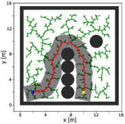
(a)

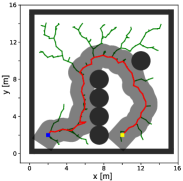
(b)

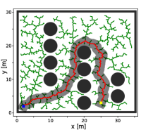
(c)

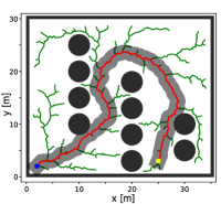
(d)

Figure 2: Visualization of the global planning results generated by Baseline 3 and the proposed method in two environments. maxIter is set to 2000 and 3000 for Env. 1 and Env. 2, respectively. The blue and yellow squares represent the start and goal position. The black circles represent the known obstacles. The green lines depict the edges of the tree $\mathcal{E}$ appended during the planning process. The red line depict the final reference path. The shaded areas in gray represent the local collision-free set $\mathcal{B}_{t}$ that the robot will sense while following the reference path.

After the global planning cycle described in Sec. IV, the local controller $\pi$ tracks the waypoints ${\bm{x}}_{i}^{\text{ref}}\in\mathcal{P}$ enabling the robot to navigate towards the goal. During navigation, the robot utilizes its onboard sensor to create a map of the environment and detect obstacles on-the-fly. The environment may contain unknown obstacles that were not considered during the global planning phase. The local controller must ensure that the robot remains within the true collision-free set $\mathcal{S}$ during navigation, avoiding collisions with both known and unknown obstacles.

Two main strategies exist for designing safety-critical controllers in such cases. The first strategy treats unmeasured space as free space and focuses on avoiding previously known and newly detected obstacles. A common approach to this problem is the use of CBFs to formally guarantee collision avoidance. CBF-based quadratic programs (CBF-QPs) have emerged as a popular and computationally efficient method for enforcing safety-critical control objectives [2, 18]. However, a notable challenge emerges under limited sensing capabilities. Specifically, if an obstacle is detected in close proximity to the robot, particularly during rotational maneuvers, the CBF-QP may become infeasible as there might not be a feasible solution to avoid the obstacle due to the proximity and the robot’s dynamics.

The second strategy treats the unmeasured space as an unsafe set and only controls the robot within the collision-free space sensed by the onboard sensor. The GateKeeper algorithm [12] is a recent advance in this strategy, acting as a safety filter between the planner and the low-level controller. If the nominal trajectory enters the unmeasured space, GateKeeper executes a backup controller to ensure the robot remains within the known collision-free space. While this strategy prevents collisions with hidden obstacles if a valid backup controller exists, the main challenge arises when the nominal global planner is agnostic to the robot’s local sensing capabilities. In such cases, GateKeeper frequently executes the backup controller and requires global replanning based on the updated environmental information, which can significantly degrade the system’s operational efficiency.

Assuming a safety-critical local controller $\pi$ interfacing with the global planner, we can now prove the properties of the resulting path from our proposed planner:

Theorem 3.

Let $p^{\textup{ref}}:\mathcal{X}\to\mathcal{P}$ be the global reference path generated by the Visibility-Aware RRT* (Alg. 1), represented by a set of waypoints $\mathcal{P}=\{{\bm{x}}^{\textup{ref}}_{i}\}_{i=0}^{N}$. If there exists a local tracking controller $\pi$ with a maximum tracking error $\epsilon$ that can track the trajectory between consecutive waypoints, then the reference path $p^{\textup{ref}}$, when tracked by such controller $\pi$, is both collision-free and visibility-aware.

Proof.

The trajectory $\bm{\sigma}_{i}$ connecting consecutive waypoints ${\bm{x}}^{\textup{ref}}_{i}$ and ${\bm{x}}^{\textup{ref}}_{i+1}$ is generated by the LQR-CBF-Steer function. By construction, each trajectory satisfies both collision avoidance (20) and visibility (28) CBF constraints, considering the robot radius $r_{\text{r}}$ and the maximum tracking error $\epsilon$. Since (20) is satisfied, the trajectories remain within the set $\mathcal{C}_{\textup{col}}=\{{\bm{x}}\in\mathcal{X}:h_{\textup{col}}({\bm{x}})\geq 0\}$, where $h_{\textup{col}}$ is given by (19). This guarantees that the local controller $\pi$ follows the trajectory $\bm{\sigma}_{i}$ with a maximum tracking error of $\epsilon$ to remain collision-free (13). Moreover, since (28) is met, the local controller $\pi$ forces the robot to move along position trajectories $\bm{\sigma}_{i}$ from which the critical point (according to Definition 5) is visible before it is reached. This guarantees that the local controller $\pi$ can detect and avoid hidden obstacles that, in the worst-case scenario, are placed at the boundary of the local safe set $\mathcal{B}_{t}$. Consequently, the local controller $\pi$ can keep the robot within the known local collision-free sets $\mathcal{B}_{t}$ while tracking the reference path $p^{\textup{ref}}$, satisfying the visibility-aware condition (16). ∎

VI RESULTS

In this section, we evaluate the proposed visibility-aware RRT* through simulation results in two distinct environments. We demonstrate that our approach can address the challenges faced by both CBF-QP and GateKeeper methods, providing a safe and efficient solution for navigating in environments with unknown obstacles, which visibility-agnostic planners fail to achieve.

The first environment (Env. 1) spans an area of 15 m $\times$ 15 m, while the second one (Env. 2) covers a larger area of 35 m $\times$ 30 m. Both environments contain known obstacles that prevent the robot from taking a straight-line path to the goal. The onboard sensor’s FOV $\theta_{\text{fov}}$ and the sensing range $l_{\text{range}}$ are set to $70^{\circ}$ and 3 m, respectively, unless otherwise specified.

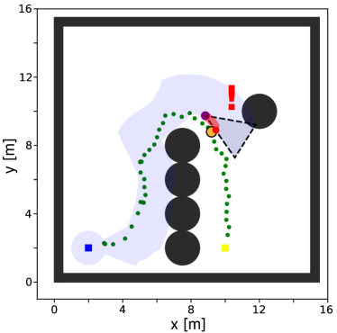
(a)

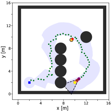
(b)

Figure 3: Visualization of the CBF-QP experiments for Env. 1 with a $45^{\circ}$ FOV. The reference waypoints (green dots) correspond to the paths in Fig. 2(a) and Fig. 2(b). The blue shaded areas represent the actual local collision-free set $\mathcal{B}_{t}$ collected from the onboard sensor. The orange circles are the hidden obstacles $\mathcal{H}$ and the red dots indicate the detection points of these hidden obstacles. (a) The CBF-QP becomes infeasible when it detects the hidden obstacle, as the robot is already within an unsafe distance to perform collision avoidance. (b) Tracking the reference path from our method, the CBF-QP successfully avoids the hidden obstacle and reaches the goal.

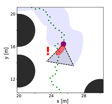
(a)

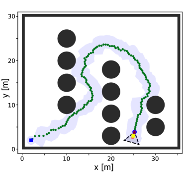
(b)

Figure 4: Visualization of the GateKeeper experiments for Env. 2. The reference waypoints correspond to the paths in Fig. 2(c) and Fig. 2(d). Red shaded areas depict the subsequent nominal trajectories at the robot’s position. (a) The GateKeeper executes a stop command as the nominal trajectory is deemed unsafe, where the trajectory lies outside of the local collision-free set $\mathcal{B}_{t}$. Consequently, global replanning is required from the current position. (b) By tracking our reference path, the GateKeeper successfully navigates to the goal without violating visibility constraint.

TABLE I: (left) Collision rates of the CBF-QP controller tracking reference paths generated by different planners in two environments with varying FOV angles. (right) Percentage of reference paths that triggered the execution of the backup controller in the GateKeeper algorithm, indicating the need for global replanning from scratch. Note that Baseline 1 is a deterministic planner, there is only one reference path tested.

Controller	CBF-QP				GateKeeper
Env.	Env. 1		Env. 2		Env. 1	Env. 2
FOV	$45^{\circ}$	$70^{\circ}$	$45^{\circ}$	$70^{\circ}$	$70^{\circ}$	$70^{\circ}$
Baseline 1	100%	0%	0%	0%	100%	100%
Baseline 2	5%	3%	13%	9%	23%	32%
Baseline 3	4%	0%	1%	1%	18%	13%
Ours	0%	0%	0%	0%	1%	0%

We compare four planning methods in our experiments: (i) The A* algorithm with an obstacle distance cost [19] (Baseline 1), (ii) the standard LQR-RRT* algorithm [13] (Baseline 2), (iii) our proposed method without the visibility constraint (Baseline 3), and (iv) the propsed visibility-aware RRT*. To highlight the effect of the visibility constraint, we illustrate the reference paths generated by Baseline 3 and our method in Fig. 2. The results demonstrate that our method maintains fewer nodes in the tree compared to Baseline 3, as it only extends the nodes that satisfy the visibility constraint. This selective expansion leads to a more computationally efficient exploration of the configuration space [20]. Furthermore, the final reference path generated by our method tends to take shallower turns around the known obstacles. This behavior complements the local tracking controller by providing a path that allows it to detect and avoid potential hidden obstacles.

To demonstrate the effectiveness of the generated paths when interfacing with the local tracking controllers, we employ two types of controllers to track the paths as discussed in Sec. V: a CBF-QP controller and the GateKeeper algorithm. We employ the dynamic unicycle model, which takes translational acceleration as input instead of velocity, in our tracking controllers to effectively capture the realistic dynamics and constraints of the robot [21].

First, we evaluate the safety perspective of the reference path when it interfaces with the CBF-QP controller. We formulate the CBF-QP as in [21], using the dynamic unicycle model, incorporating a CBF constraint for collision avoidance. In this experiment, we test two different FOV angles: $45^{\circ}$ and $70^{\circ}$. For Baseline 1, which is a deterministic planner, we run the algorithm once and for Baselines 2-3 and our proposed method, which are sampling-based planners, we generate 100 reference paths for each setting. After the planning phase, we place unknown obstacles near the known obstacles. Then, we evaluate whether the CBF-QP controller can successfully navigate the robot to the goal without collisions. One example of this experiment is shown in Fig. 3. The results, summarized in Table I, demonstrate that even with a safety-critical controller using a valid CBF for collision avoidance, safety cannot be guaranteed if the planner does not consider the robot’s perception limitations. This is because the robot detects the hidden obstacle too late, leaving no feasible solution for the CBF-QP to avoid the obstacle. This aspect becomes more prominent as the sensing capability becomes more limited. In contrast, the visibility-aware paths generated by our method can effectively complement the local tracking controller, ensuring safe navigation even in the presence of limited perception.

Next, we investigate the efficiency of the reference paths when interfacing with the GateKeeper algorithm [12]. GateKeeper assesses the safety of the nominal trajectory and decides whether to follow it or execute a backup controller, which, in this case, is a stop command. If the next nominal trajectory is deemed unsafe, meaning the robot might not be able to completely stop within the known collision-free space given its control authority, GateKeeper opts not to follow the nominal trajectory. Instead, it executes the backup controller and subsequently plans for global path again. We evaluate the percentage of the same set of reference paths that trigger the execution of the backup controller, indicating that the path was inefficient for navigation. One example of this experiment is shown in Fig. 4. The results, presented in Table I, show that visibility-aware RRT* significantly reduces the need for replanning compared to the baseline planners. This demonstrates that the proposed method generates reference paths that are more efficient for navigation by minimizing the frequency of replanning required when used with controllers that treat unmeasured space as an unsafe set.

VII CONCLUSION

In this paper, we considered that safety may not be guaranteed for robots with limited perception capabilities navigating in unknown environments, even when using safety-critical controllers. To address this challenge, we introduced the Visibility-Aware RRT* algorithm, which generates a global reference path that is both collision-free and visibility-aware, enabling the tracking controller to avoid hidden obstacles at all times. We introduced the visibility CBF to encode the robot’s visibility limitations, utilizing its constraint as a termination criterion during the steering process, alongside a standard collision avoidance CBF constraint. We also proved that our algorithm ensures the satisfaction of visibility constraints by the local controller, and we evaluated the performance of the integrated path planner with two different controllers via simulations. The results indicated that our method outperformed all other compared baselines in both safety and efficiency aspects.

References

- [1] J. G. da Silva Neto, P. J. da Lima Silva, F. Figueredo, J. M. X. N. Teixeira, and V. Teichrieb, “Comparison of RGB-D sensors for 3D reconstruction,” in Symposium on Virtual and Augmented Reality (SVR), 2020, pp. 252–261.
- [2] A. D. Ames, J. W. Grizzle, and P. Tabuada, “Control barrier function based quadratic programs with application to adaptive cruise control,” in IEEE Conference on Decision and Control, 2014, pp. 6271–6278.
- [3] I. Spasojevic, V. Murali, and S. Karaman, “Perception-aware time optimal path parameterization for quadrotors,” in IEEE International Conference on Robotics and Automation, 2020, pp. 3213–3219.
- [4] B. Zhou, J. Pan, F. Gao, and S. Shen, “RAPTOR: Robust and Perception-Aware Trajectory Replanning for Quadrotor Fast Flight,” IEEE Transactions on Robotics, vol. 37, no. 6, pp. 1992–2009, 2021.
- [5] V. Murali, I. Spasojevic, W. Guerra, and S. Karaman, “Perception-aware trajectory generation for aggressive quadrotor flight using differential flatness,” in American Control Conference (ACC), 2019, pp. 3936–3943.
- [6] R. M. Bena, C. Zhao, and Q. Nguyen, “Safety-Aware Perception for Autonomous Collision Avoidance in Dynamic Environments,” IEEE Robotics and Automation Letters, vol. 8, no. 12, pp. 7962–7969, 2023.
- [7] X. Chen, Y. Zhang, B. Zhou, and S. Shen, “APACE: Agile and Perception-Aware Trajectory Generation for Quadrotor Flights,” in IEEE International Conference on Robotics and Automation (ICRA), 2024.
- [8] G. Oriolo, M. Vendittelli, L. Freda, and G. Troso, “The SRT method: randomized strategies for exploration,” in IEEE International Conference on Robotics and Automation (ICRA), 2004, pp. 4688–4694.
- [9] A. D. Ames, S. Coogan, M. Egerstedt, G. Notomista, K. Sreenath, and P. Tabuada, “Control Barrier Functions: Theory and Applications,” in European Control Conference (ECC), 2019, pp. 3420–3431.
- [10] W. Xiao and C. Belta, “Control Barrier Functions for Systems with High Relative Degree,” in IEEE Conference on Decision and Control (CDC), 2019, pp. 474–479.
- [11] Q. Nguyen and K. Sreenath, “Exponential Control Barrier Functions for enforcing high relative-degree safety-critical constraints,” in American Control Conference (ACC), 2016, pp. 322–328.
- [12] D. Agrawal, R. Chen, and D. Panagou, “gatekeeper: Online Safety Verification and Control for Nonlinear Systems in Dynamic Environments,” in IEEE/RSJ International Conference on Intelligent Robots and Systems (IROS), 2023, pp. 259–266.
- [13] A. Perez, R. Platt, G. Konidaris, L. Kaelbling, and T. Lozano-Perez, “LQR-RRT*: Optimal sampling-based motion planning with automatically derived extension heuristics,” in IEEE International Conference on Robotics and Automation (ICRA), 2012, pp. 2537–2542.
- [14] S. Karaman and E. Frazzoli, “Sampling-based algorithms for optimal motion planning,” The International Journal of Robotics Research, vol. 30, no. 7, pp. 846–894, 2011.
- [15] G. Yang, M. Cai, A. Ahmad, A. Prorok, R. Tron, and C. Belta, “LQR-CBF-RRT*: Safe and Optimal Motion Planning,” in arXiv preprint arXiv:2304.00790, 2023.
- [16] G. Yang, B. Vang, Z. Serlin, C. Belta, and R. Tron, “Sampling-based Motion Planning via Control Barrier Functions,” in International Conference on Automation, Control and Robots, 2019, pp. 22–29.
- [17] H. Parwana and D. Panagou, “Recursive Feasibility Guided Optimal Parameter Adaptation of Differential Convex Optimization Policies for Safety-Critical Systems,” in IEEE International Conference on Robotics and Automation (ICRA), 2022, pp. 6807–6813.
- [18] M. Jankovic and M. Santillo, “Collision Avoidance and Liveness of Multi-agent Systems with CBF-based Controllers,” in IEEE Conference on Decision and Control (CDC), 2021, pp. 6822–6828.
- [19] T. Kim, S. Lim, G. Shin, G. Sim, and D. Yun, “An Open-Source Low-Cost Mobile Robot System With an RGB-D Camera and Efficient Real-Time Navigation Algorithm,” IEEE Access, vol. 10, pp. 127 871–127 881, 2022.
- [20] C. Tao, H. Kim, H. Yoon, N. Hovakimyan, and P. Voulgaris, “Control Barrier Function Augmentation in Sampling-based Control Algorithm for Sample Efficiency,” in American Control Conference (ACC), 2022, pp. 3488–3493.
- [21] H. Parwana, M. Black, B. Hoxha, H. Okamoto, G. Fainekos, D. Prokhorov, and D. Panagou, “Feasible Space Monitoring for Multiple Control Barrier Functions with application to Large Scale Indoor Navigation,” in arXiv preprint arXiv.2312.07803, 2023.