Nitsche stabilized Virtual element approximations for a Brinkman problem with mixed boundary conditions

Abstract

In this paper, we formulate, analyse and implement the discrete formulation of the Brinkman problem with mixed boundary conditions, including slip boundary condition, using the Nitsche’s technique for virtual element methods. The divergence conforming virtual element spaces for the velocity function and piecewise polynomials for pressure are approached for the discrete scheme. We derive a robust stability analysis of the Nitsche stabilized discrete scheme for this model problem. We establish an optimal and vigorous a priori error estimates of the discrete scheme with constants independent of the viscosity. Moreover, a set of numerical tests demonstrates the robustness with respect to the physical parameters and verifies the derived convergence results.

1 Introduction and problem statement

We are interested in the numerical approximation by the virtual element method of the Brinkman system with mixed boundary conditions, that is, Dirichlet conditions on one part on the boundary and slip conditions on the rest of the boundary. These boundary conditions, representing the inflow/outflow in domain, and flow through the boundary wall as well fluid slipping along the boundary wall, have been introduced in the several applications such as water treatment, reverse osmosis and so on. The Brinkman equations can be seen as an extension of Darcy’s law to describe the laminar flow behavior of a viscous fluid within a porous material with possibly heterogeneous permeability, so that the flow is dominated by Darcy regime on a part of the domain and by Stokes on the other parts of the domain. In the last years, the numerical solution of this system has acquired great interest due to high practical importance in different areas, including several industrial and environmental applications, such as, filtering porous layers, oil reservoirs, the study of foams, among others.

The virtual element method (VEM) introduced in daveiga-b13 , belong to the so-called polytopal methods for solving PDEs by using general polygonal/polyhedral meshes. These methods have received substantial attention in the last years, for instance, hybrid high order method HHO1 ; HHObook ; droniou2 ; droniou3 , discontinuous Galerkin method Cangiani14 ; paola2021 ; zhao1 , mimetic finite difference method Mimetic2014 , virtual element method huang1 ; MR4510898 ; MR4586821 The VEM can be seen as an extension of Finite Elements Method (FEM) to polygonal or polyhedral decompositions. The VEM has been applied for different problems in fluid mechanics, see for instance, ABMV2014 ; BMVjsc19 ; BLVm2an17 ; BLVsinum18 ; CGima17 ; CGSm3as17 ; GSm3as21 ; GMScalcolo18 ; Mora21imajna ; vacca17 and the references therein.

In GMScalcolo18 , virtual element method for a pseudostress-velocity formulation for the nonlinear Brinkman flow has been introduced. The stream virtual element method has been introduced and analyzed in Mora21imajna . In this case, the problem is written as a single equation in terms of the stream function of the velocity field by using the incompressibility condition, and optimal error estimates, independent of the viscosity parameter, are obtained. In BLVm2an17 ; BLVsinum18 the authors have introduced a novel divergence-free virtual element method for solving the Stokes and Navier-Stokes problems. This method has been used in vacca17 for solving the Brinkman problem with homogeneous Dirichlet boundary conditions, and the error estimates independent of the model parameters are written. Moreover, we also mention recent works for the numerical discretization of the Brinkman problem by finite element method anaya16 ; anaya17 ; meddahi1 ; fila1 .

The so-called Nitsche methods can be regarded as a stabilization technique where some terms are added to the variational formulation so that the boundary conditions can be incorporated in a weak form. One of the main advantages of the Nitsche method is its versatility. It can be applied to a wide range of partial differential equations, including elliptic, parabolic, and hyperbolic equations. For instance, finite element discretizations with Nitsche method has evolved to handle general boundary conditions juntunen2009nitsche , including interface problems hansbo2005nitsche , unilateral and frictional contact chouly2013nitsche ; chouly2018unbiased , or membrane filtration processes carro_ijnmf24 , among others. On each reference, we observe that a properly formulated penalty terms in the Nitsche method ensure consistency and stability of the numerical solution, even for complex problems and irregular domains. This stability property is crucial for obtaining reliable and accurate results in practical simulations. Moreover, the Nitsche method can be relatively straightforward to implement compared to other approaches for enforcing boundary conditions. Its penalty-based formulation simplifies the incorporation of boundary conditions into the variational formulation of the problem. By the nature of the method, this can be seamlessly integrated with modern numerical techniques such as adaptive mesh refinement, parallel computing, higher-order finite elements, or virtual elements method. In the latter, the literature regarding Nitsche’s method is scarce, with a recent contribution by bertoluzza2022weakly . Here, the authors study the extension to virtual elements of the Lagrange multiplier method, in its stabilized formulation as proposed by Barbosa and Hughes barbosa1991finite , and the Nitsche method nitsche91 . They proved stability and optimal error estimates, under custom conditions on the stabilization parameters. The results are extended for two and three dimensional geometries with curved domains, where the numerical experiments assess the performance of the method, suggesting a viable alternative to the corresponding scheme in the finite element method.

In the present contribution we propose a Nitsche method for the Brinkman system with mixed boundary conditions. We consider Dirichlet condition on a part of the boundary and slip conditions on the rest of the boundary. This approach have been employed in several Navier-Stokes models to impose a slip boundary condition. We have for example the work from urquiza2014weak , where they compare the Lagrange multiplier and Nitsche’s method for the weakly imposition of the slip boundary condition on curved domains. Recently, in gjerde2022nitsche the authors study the weak imposition of the slip-boundary through Nitsche’s method and projected normals between the computational and the continuous domain, and also explore the well-known Babuška-Sapondzhyan Paradox. The type of conditions behind the models presented in the aforementioned works are important in different areas for fluid flow problems. In particular, these boundary conditions appears naturally in the analysis of numerical methods for desalinization processes, filtration, among others. For that reason, in this work, we extend the results presented in vacca17 for the new model problem. Unlike the Dirichlet boundary conditions, the slip-boundary conditions are inadequate to impose strongly for discrete solution. This drawback is due to the unavailability of the degrees of freedom for the normal component and normal derivative of the function on the boundary in the discrete space. It is well know that different strategies can be considered for imposing mixed conditions, including slip conditions, such as, Lagrange multiplier method. However, we here propose a symmetric discrete variational formulation by adding Nitsche terms in order to incorporate the boundary conditions considered in the model problem. Moreover, we discretize the problem, by using the virtual element method presented in BLVm2an17 for the Stokes problem. We define a new Nitsche term to impose the slip boundary condition for the discrete scheme using the piecewise polynomial projection on each polygon $K$ (in the mesh) on the boundary. We establish that the discrete problem is well posed by proving a global inf-sup condition and we write stability by using appropriate mesh-parameter dependent norms. Under rather mild assumptions on the polygonal meshes and by using interpolation estimates, the convergence rate is proved to be optimal in terms of the mesh size $h$. We would like to emphasis that the constants in the derivation of error estimates are independent of the physical parameters in this model problem. The trace inequality for the piecewise polynomials are utilised in the analysis in order to prove the stability. In summary, the advantages of the proposed Nitsche VEM method for the Brinkman problem are, on the one hand, the possibility to use general polygonal meshes, and on the other hand, the possibility of an easy imposition of general boundary conditions, including non homogeneous Dirichlet conditions, slip conditions, among others.

The rest of the paper is organized as follows: in Section 2 we introduce the variational formulation of the Brinkman equations with mixed boundary conditions. In Section 3 we present the virtual element discretization of arbitrary order $k\geq 2$ with Nitsche’s technique. The existence, uniqueness and stability results of the discrete formulation by using a global inf-sup condition is presented in Section 4. In Section 5 we obtain error estimates for the velocity and pressure fields. Section 6 is devoted to analyze, through several numerical experiments, the performance and robustness of the proposed Nitsche method.

In this article, we will employ standard notations for Sobolev spaces, norms and seminorms. In addition, we will denote by $C$ a generic constant independent of the mesh parameter $h$ and model parameters, which may take different values in different occurrences.

2 Governing equations

Let $\Omega$ be an open, bounded subset of $\mathbb{R}^{2}$ having Lipschitz–continuous boundary, such that $\partial\Omega=\bar{\Gamma}_{D}\cup\bar{\Gamma}_{N}$, and $\Gamma_{D}\cap\Gamma_{N}=\emptyset$. The boundary subdomain $\Gamma_{D}$ represents a part of $\partial\Omega$ where a fixed value for the velocity (Dirichlet boundary) is given, while $\Gamma_{N}$ denotes a subdomain where we have a slip boundary condition. An example of such domain is depicted in Figure 2.1. Thus, the system of interest can be written as the following problem. Given the body force $\boldsymbol{f}\in[L^{2}(\Omega)]^{2}$ and boundary condition $\boldsymbol{g}\in[H^{1/2}(\Gamma_{D})]^{2}$, find the fluid velocity $\boldsymbol{u}$ and fluid pressure $p$, such that

$$\mathbb{K}^{-1}\boldsymbol{u}-\nu\mathop{\mathrm{div}}\nolimits(\boldsymbol{\varepsilon}(\boldsymbol{u}))+\nabla p =\boldsymbol{f} \text{in $\Omega$},$$ (2.1)

$$\nabla\cdot\boldsymbol{u} =0 \text{in $\Omega$},$$ (2.2)

$$\boldsymbol{u} =\boldsymbol{g} \text{on $\Gamma_{D}$},$$ (2.3)

$$(\boldsymbol{\varepsilon}(\boldsymbol{u})\boldsymbol{n})\cdot\boldsymbol{t}=0,\quad\text{and}\quad\boldsymbol{u}\cdot\boldsymbol{n} =0 \text{on $\Gamma_{N}$},$$ (2.4)

where $\nu$ is the viscosity of the fluid, $\boldsymbol{\varepsilon}(\boldsymbol{v}):=\frac{1}{2}(\nabla\boldsymbol{v}+(\nabla\boldsymbol{v})^{t})$ is the symmetric derivative, $\mathbb{K}$ is a bounded, symmetric, and positive definite tensor describing the permeability properties of the Brinkman region, and $\boldsymbol{n}:=(n_{1},n_{2})^{\texttt{t}}$ and $\boldsymbol{t}$ are unit normal and tangent on the boundary $\Gamma_{N}$, respectively, with $\boldsymbol{t}:=(-n_{2},n_{1})^{\texttt{t}}$.

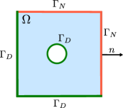
Figure 2.1: Sample geometry of the considered Brinkman domain with mixed boundary conditions.

In order to obtain the weak form of the governing equations, let us introduce the functional spaces for the velocity and pressure.

$$\mathbf{V}:=\{\boldsymbol{v}\in[H^{1}(\Omega)]^{2}:\boldsymbol{v}\cdot\boldsymbol{n}=0\text{ on }\Gamma_{N},\boldsymbol{v}=\boldsymbol{0}\text{ on }\Gamma_{D}\}\qquad\text{and}\qquad Q:=L^{2}_{0}(\Omega).$$

We first state the assumptions on the physical parameters used throughout this paper. The permeability tensor holds the positive definiteness for all $\boldsymbol{v}\in\mathbf{V}$, that is there exist $\kappa_{1},\kappa_{2}>0$ such that

$$0<\kappa_{1}\|\boldsymbol{v}\|_{0,\Omega}^{2}\leq(\mathbb{K}^{-1}\boldsymbol{v},\boldsymbol{v})_{0,\Omega}\leq\kappa_{2}\|\boldsymbol{v}\|_{0,\Omega}^{2}<\infty,$$

and we also assume that $0<\nu\leq 1$.

Next, we test the corresponding equations in (2.1)-(2.2) and using integration by parts and the fact that $\boldsymbol{v}\in\mathbf{V}$, we have

$$\int_{\Omega}\mathbb{K}^{-1}\boldsymbol{u}\cdot\boldsymbol{v}+\nu\int_{\Omega}\boldsymbol{\varepsilon}(\boldsymbol{u}):\boldsymbol{\varepsilon}(\boldsymbol{v})-\int_{\Omega}p\mathop{\mathrm{div}}\nolimits\boldsymbol{v}-\int_{\Gamma_{N}}(\nu\boldsymbol{\varepsilon}(\boldsymbol{u})-p\mathbb{I})\boldsymbol{n}\cdot\boldsymbol{v}\,\mathrm{d}s =\int_{\Omega}\boldsymbol{f}\cdot\boldsymbol{v}\qquad\forall\boldsymbol{v}\in\mathbf{V},$$

$$-\int_{\Omega}\mathop{\mathrm{div}}\nolimits\boldsymbol{u}\,q =0\qquad\qquad\quad\forall q\in Q.$$

To impose the Dirichlet condition for the continuous solution $\boldsymbol{u}$, we define the Sobolev space

$$\mathbf{V}_{g}:=\{\boldsymbol{v}\in\mathbf{V}:\boldsymbol{v}\cdot\boldsymbol{n}=0\text{ on }\Gamma_{N},\boldsymbol{v}=\boldsymbol{g}\text{ on }\Gamma_{D}\}.$$

The boundary term in the weak formulation for $\boldsymbol{u}\in\mathbf{V}_{g}$, $\boldsymbol{v}\in\mathbf{V}$ and $p\in Q$ can be computed by splitting the terms in terms of tangential and normal components ($\boldsymbol{w}=(\boldsymbol{w}\cdot\boldsymbol{n})\boldsymbol{n}+(\boldsymbol{w}\cdot\boldsymbol{t})\boldsymbol{t}$) as,

$$\int_{\Gamma_{N}}(\nu\boldsymbol{\varepsilon}(\boldsymbol{u})-p\mathbb{I})\boldsymbol{n}\cdot\boldsymbol{v}\,\mathrm{d}s =\int_{\Gamma_{N}}\Big{(}(\boldsymbol{n}^{t}(\nu\boldsymbol{\varepsilon}(\boldsymbol{u})\boldsymbol{n}))(\boldsymbol{v}\cdot\boldsymbol{n})+(\boldsymbol{t}^{t}(\nu\boldsymbol{\varepsilon}(\boldsymbol{u})\boldsymbol{n}))(\boldsymbol{v}\cdot\boldsymbol{t})-p(\boldsymbol{v}\cdot\boldsymbol{n})\Big{)}\,\mathrm{d}s$$

$$=\int_{\Gamma_{N}}(\boldsymbol{t}^{t}(\nu\boldsymbol{\varepsilon}(\boldsymbol{u})\boldsymbol{n}))(\boldsymbol{v}\cdot\boldsymbol{t})\,\mathrm{d}s=0,$$

where we have also used the boundary condition $\eqref{bc:Gamma}$.

Thus, the weak formulation of the problem is stated as: find $\boldsymbol{u}\in\mathbf{V}_{g}$ and $p\in Q$ such that

$$m(\boldsymbol{u},\boldsymbol{v})+a(\boldsymbol{u},\boldsymbol{v})+b(\boldsymbol{v},p) =F(\boldsymbol{v}) \quad\forall\boldsymbol{v}\in\mathbf{V},$$ (2.5a)

$$b(\boldsymbol{u},q) =0 \quad\forall q\in Q,$$ (2.5b)

where the corresponding bilinear forms and the linear functional are introduced as follows

$$m(\boldsymbol{u},\boldsymbol{v}):=\int_{\Omega}\mathbb{K}^{-1}\boldsymbol{u}\cdot\boldsymbol{v},\qquad a(\boldsymbol{u},\boldsymbol{v}):=\nu\int_{\Omega}\boldsymbol{\varepsilon}(\boldsymbol{u}):\boldsymbol{\varepsilon}(\boldsymbol{v}),$$

$$b(\boldsymbol{v},q):=-\int_{\Omega}q\mathop{\mathrm{div}}\nolimits\boldsymbol{v},\quad\text{and}\quad F(\boldsymbol{v}):=\int_{\Omega}\boldsymbol{f}\cdot\boldsymbol{v}.$$

Now, we introduce the parameter dependent norm for all $\boldsymbol{v}\in\mathbf{V}$ as follows:

$${\left|\kern-1.07639pt\left|\kern-1.07639pt\left|\boldsymbol{v}\right|\kern-1.07639pt\right|\kern-1.07639pt\right|}_{\mathbf{V}}^{2}:=\|\mathbb{K}^{-1/2}\boldsymbol{v}\|_{0,\Omega}^{2}+\nu\|\boldsymbol{\varepsilon}(\boldsymbol{v})\|_{0,\Omega}^{2}+\|\mathop{\mathrm{div}}\nolimits\boldsymbol{v}\|_{0,\Omega}^{2}.$$

Defining the kernel space as

$$\mathbf{Z}:=\{\boldsymbol{v}\in\mathbf{V}:b(\boldsymbol{v},q)=0\quad\forall q\in Q\}=\{\boldsymbol{v}\in\mathbf{V}:\mathop{\mathrm{div}}\nolimits\boldsymbol{v}=0\},$$

then we have the following properties of the bilinear forms:

$$m(\boldsymbol{u},\boldsymbol{v})\leq{\left|\kern-1.07639pt\left|\kern-1.07639pt\left|\boldsymbol{u}\right|\kern-1.07639pt\right|\kern-1.07639pt\right|}_{\mathbf{V}}{\left|\kern-1.07639pt\left|\kern-1.07639pt\left|\boldsymbol{v}\right|\kern-1.07639pt\right|\kern-1.07639pt\right|}_{\mathbf{V}},\qquad a(\boldsymbol{u},\boldsymbol{v})\leq{\left|\kern-1.07639pt\left|\kern-1.07639pt\left|\boldsymbol{u}\right|\kern-1.07639pt\right|\kern-1.07639pt\right|}_{\mathbf{V}}{\left|\kern-1.07639pt\left|\kern-1.07639pt\left|\boldsymbol{v}\right|\kern-1.07639pt\right|\kern-1.07639pt\right|}_{\mathbf{V}}\quad\forall\boldsymbol{u},\boldsymbol{v}\in\mathbf{V},$$

$$b(\boldsymbol{v},q)\leq{\left|\kern-1.07639pt\left|\kern-1.07639pt\left|\boldsymbol{v}\right|\kern-1.07639pt\right|\kern-1.07639pt\right|}_{\mathbf{V}}\|q\|_{Q}\quad\forall\boldsymbol{v}\in\mathbf{V},q\in Q,\qquad F(\boldsymbol{v})\leq\|\boldsymbol{f}\|_{\mathbf{V}^{*}}{\left|\kern-1.07639pt\left|\kern-1.07639pt\left|\boldsymbol{v}\right|\kern-1.07639pt\right|\kern-1.07639pt\right|}_{\mathbf{V}}\quad\forall\boldsymbol{v}\in\mathbf{V},$$

$$m(\boldsymbol{v},\boldsymbol{v})+a(\boldsymbol{v},\boldsymbol{v})\geq{\left|\kern-1.07639pt\left|\kern-1.07639pt\left|\boldsymbol{v}\right|\kern-1.07639pt\right|\kern-1.07639pt\right|}_{\mathbf{V}}^{2}\quad\forall\boldsymbol{v}\in\mathbf{Z},\quad\text{and}\quad\sup_{(0\neq)\boldsymbol{v}\in\mathbf{V}}\frac{b(\boldsymbol{v},q)}{{\left|\kern-1.07639pt\left|\kern-1.07639pt\left|\boldsymbol{v}\right|\kern-1.07639pt\right|\kern-1.07639pt\right|}_{\mathbf{V}}}\geq\beta\left\|q\right\|_{Q}\qquad\forall q\in Q,$$

where $\left\|q\right\|_{Q}:=\|q\|_{0,\Omega}$ and $\|\boldsymbol{f}\|_{\mathbf{V}^{*}}:=\sup_{\boldsymbol{v}\in\mathbf{V}}\frac{F(\boldsymbol{v})}{{\left|\kern-0.75346pt\left|\kern-0.75346pt\left|\boldsymbol{v}\right|\kern-0.75346pt\right|\kern-0.75346pt\right|}_{\mathbf{V}}}.$

Using the ellipticity of $m(\cdot,\cdot)+a(\cdot,\cdot)$ on $\mathbf{Z}$, and the inf-sup condition of $b(\cdot,\cdot)$, and continuity of the bilinear forms of $m(\cdot,\cdot)$, $a(\cdot,\cdot)$, $b(\cdot,\cdot)$ and continuity of the linear functional $F(\cdot)$, we have the well posedness of the weak formulation (2.5) (refer boffi13 ; brenner08 ).

Lemma 2.1

The continuous solution $(\boldsymbol{u},p)\in\mathbf{V}_{g}\times Q$ of formulation (2.5) holds the following bound, for a constant $C$ (independent of $\nu,\,\mathbb{K}$),

$${\left|\kern-1.07639pt\left|\kern-1.07639pt\left|\boldsymbol{u}\right|\kern-1.07639pt\right|\kern-1.07639pt\right|}_{\mathbf{V}}+\|p\|_{Q}\leq C\|\boldsymbol{f}\|_{\mathbf{V}^{*}}.$$ (2.6)

3 Virtual element approximation

In this section we construct a VEM for solving the Brinkman problem with mixed boundary conditions using Nitsche’s technique. We start denoting by $\{{\mathcal{T}}_{h}\}_{h}$ a sequence of partitions into polygons of the domain $\Omega$. The elements in $\mathcal{T}_{h}$ are denoted as $K$, and edges by $e$. Let $h_{K}$ denote the diameter of the element $K$ and $h:=\max_{K\in{\mathcal{T}}_{h}}h_{K}$ the maximum of the diameters of all the elements of the mesh. By $N^{v}_{K}$ we denote the number of vertices in the polygon $K$, $N^{e}_{K}$ stands for the number of edges on $\partial K$, and $e$ is a generic edge of $\mathcal{T}_{h}$. We denote by $\boldsymbol{n}_{K}^{e}$ the unit normal pointing outwards $K$ and by $\boldsymbol{t}^{e}_{K}$ the unit tangent vector along $e$ on $K$, and $V_{i}$ represents the $i^{th}$ vertex of the polygon $K$.

Next, we denote the sets of all boundary edges as $\mathcal{E}_{h}(\Omega)$ and denote the edges on the Dirichlet boundary as $\mathcal{E}_{h}^{D}:=\Gamma_{D}\cap\mathcal{E}_{h}(\Omega)$ and edges on the other boundary as $\mathcal{E}_{h}^{N}:=\Gamma_{N}\cap\mathcal{E}_{h}(\Omega)$.

In addition, for the theoretical analysis we will make the following assumptions: there exists $C_{{\mathcal{T}}}>0$ such that, for every $h$ and every $K\in{\mathcal{T}}_{h}$, (a) the ratio between the shortest edge and $h_{K}$ is larger than $C_{{\mathcal{T}}}$; and (b) $K\in{\mathcal{T}}_{h}$ is star-shaped with respect to every point within a ball of radius $C_{{\mathcal{T}}}h_{K}$.

In what follows, we denote by $\mathbb{P}_{k}(K)$ the space of polynomials of degree up to $k$, defined locally on $K\in\mathcal{T}_{h}$. Moreover, we denote by $\mathcal{G}_{k}(K):=\nabla(\mathbb{P}_{k+1}(K))\subseteq[\mathbb{P}_{k}(K)]^{2}$ and $\mathcal{G}_{k}^{\perp}(K)\subseteq[\mathbb{P}_{k}(K)]^{2}$ the $L^{2}$-orthogonal complement to $\mathcal{G}_{k}(K)$.

3.1 Discrete spaces and degrees of freedom

The local virtual element spaces are defined for $k\geq 2$ as,

$$\tilde{\mathbf{V}}_{h}^{k}(K):=\{\boldsymbol{v}\in[H^{1}(K)\cap C^{0}(\partial K)]^{2}: -\boldsymbol{\Delta}\boldsymbol{v}-\nabla s\in\mathcal{G}_{k-2}(K)^{\perp}(\text{for some }s\in L^{2}(K)),\quad\mathop{\mathrm{div}}\nolimits\boldsymbol{v}\in\mathbb{P}_{k-1}(K),$$

$$\quad\boldsymbol{v}|_{e}\in\mathbb{P}_{k}(e)\,\forall e\in\partial K\},$$

$$\quad Q_{h}^{k}(K):=\mathbb{P}_{k-1}(K).$$

Denote the dimension of local space $\tilde{\mathbf{V}}_{h}^{k}(K)$ as $N_{\mathbf{V}}^{K}$, and dimension of $Q_{h}^{k}(K)$ as $N_{Q}^{K}$.

The local degrees of freedom $(\text{dof}_{i}^{\mathbf{V}},\,1\leq i\leq N_{\mathbf{V}}^{K})$ for space $\tilde{\mathbf{V}}_{h}^{k}(K)$ for a generic $\boldsymbol{v}_{h}\in\tilde{\mathbf{V}}_{h}^{k}(K)$ are given by

• the values of $\boldsymbol{v}_{h}$ at the vertices of the polygon $K$,

• the values of $\boldsymbol{v}_{h}$ at $k-1$ points in the interior of edges $e\in\partial K$,

• the moments of $\boldsymbol{v}_{h}$

  $$\int_{K}\boldsymbol{v}_{h}\cdot\boldsymbol{g}_{k-2}^{\perp}\quad\text{ for all }\boldsymbol{g}_{k-2}^{\perp}\in\mathcal{G}_{k-2}(K)^{\perp},$$

• for $k>1$, the moments of $\mathop{\mathrm{div}}\nolimits\boldsymbol{v}_{h}$ in $K$,

  $$\int_{K}\mathop{\mathrm{div}}\nolimits\boldsymbol{v}_{h}\,q_{k-1}\quad\text{ for all }q_{k-1}\in\mathbb{P}_{k-1}(K),$$

And for the space $Q_{h}^{k}(K)$, the degrees of freedom are

• the moments of $q_{h}$

  $$\int_{K}q_{h}\,q_{k-1}\quad\text{ for all }q_{k-1}\in\mathbb{P}_{k-1}(K).$$

Denoting the bilinear forms on each element as $a^{K}(\cdot,\cdot):=a(\cdot,\cdot)|_{K}$ for any bilinear form, we introduce the energy projection operators $\boldsymbol{\Pi}^{\boldsymbol{\nabla},k}_{K}:[H^{1}(K)]^{2}\to[\mathbb{P}_{k}(K)]^{2},\boldsymbol{\Pi}^{\boldsymbol{\varepsilon},k}_{K}:[H^{1}(K)]^{2}\to[\mathbb{P}_{k}(K)]^{2},$ and $L^{2}$ projection operator $\boldsymbol{\Pi}^{\boldsymbol{0},k}_{K}:[L^{2}(K)]^{2}\to[\mathbb{P}_{k}(K)]^{2}$ for all $K\in\mathcal{T}_{h}$ to define the computable bilinear forms,

$$\quad(\boldsymbol{\Pi}^{\boldsymbol{0},k}_{K}\boldsymbol{v}-\boldsymbol{v},\boldsymbol{r}_{k})_{0,K}=0\qquad\forall\boldsymbol{v}\in[L^{2}(K)]^{2},\boldsymbol{r}_{k}\in[\mathbb{P}_{k}(K)]^{2},$$ (3.1)

$$\forall\boldsymbol{v}\in[H^{1}(K)]^{2}, \begin{cases}(\boldsymbol{\nabla}(\boldsymbol{\Pi}^{\boldsymbol{\nabla},k}_{K}\boldsymbol{v}-\boldsymbol{v}),\boldsymbol{\nabla}\boldsymbol{r}_{k})=0\,\quad\forall\boldsymbol{r}_{k}\in[\mathbb{P}_{k}(K)]^{2},\\ \boldsymbol{\Pi}^{\boldsymbol{0},k}_{K}(\boldsymbol{\Pi}^{\boldsymbol{\nabla},k}_{K}\boldsymbol{v}-\boldsymbol{v})=\boldsymbol{0}\end{cases}$$ (3.2)

$$\forall\boldsymbol{v}\in[H^{1}(K)]^{2}, \begin{cases}a^{K}(\boldsymbol{\Pi}^{\boldsymbol{\varepsilon},k}_{K}\boldsymbol{v}-\boldsymbol{v},\boldsymbol{r}_{k})=0\,\quad\forall\boldsymbol{r}_{k}\in[\mathbb{P}_{k}(K)]^{2},\\ (\boldsymbol{\Pi}^{\boldsymbol{\varepsilon},k}_{K}\boldsymbol{v}-\boldsymbol{v},\boldsymbol{r}_{k})_{0,K}=\boldsymbol{0}\quad\forall\boldsymbol{r}_{k}\in\ker(a^{K}(\cdot,\cdot)).\end{cases}$$ (3.3)

Refer to vacca17 , we utilize the modified virtual element space for flux with the help of energy projection (3.2) as,

$${\mathbf{V}}_{h}^{k}(K):=\{\boldsymbol{v}\in[H^{1}(K)\cap C^{0}(\partial K)]^{2}: -\boldsymbol{\Delta}\boldsymbol{v}-\nabla s\in\mathcal{G}_{k}(K)^{\perp}\quad\text{for some }s\in L^{2}(K),$$

$$\quad\mathop{\mathrm{div}}\nolimits\boldsymbol{v}\in\mathbb{P}_{k-1}(K),\quad\boldsymbol{v}|_{e}\in\mathbb{P}_{k}(e)\,\forall e\in\partial K,$$

$$\quad(\boldsymbol{\Pi}^{\boldsymbol{\nabla},k}_{K}\boldsymbol{w}-\boldsymbol{w},\boldsymbol{g}_{k\backslash k-2}^{\perp})_{0,K}=0\quad\forall\,\boldsymbol{g}_{k\backslash k-2}^{\perp}\in\mathcal{G}_{k}(K)^{\perp}\backslash\mathcal{G}_{k-2}(K)^{\perp}\}.$$

The degrees of freedom for the space ${\mathbf{V}}_{h}^{k}(K)$ are same as $\tilde{\mathbf{V}}_{h}^{k}(K)$.

Remark 3.1

The space ${\mathbf{V}}_{h}^{k}(K)$ will be useful for computing the $L^{2}$-projection (3.1) onto $\mathbb{P}_{k}(K)$ to approximate the zero order term presented in bilinear form $m(\cdot,\cdot)$.

Remark 3.2

The imposition of Dirichlet boundary condition using the interpolant is not enough with complex domains, and the slip boundary conditions are not easy to impose in numerical experiments. Thus, we proceed here with the Nitsche’s technique for mixed boundary imposition.

We introduce the virtual element spaces to be used in the discretization of the Brinkman problem as:

$$\mathbf{V}_{h}^{k}:=\{\boldsymbol{v}_{h}\in[H^{1}(\Omega)]^{2}:\boldsymbol{v}_{h}|_{K}\in\mathbf{V}_{h}^{k}(K)\,\,\forall K\in\mathcal{T}_{h}\},\qquad Q_{h}^{k}:=\{q_{h}\in Q:q_{h}|_{K}\in Q_{h}^{k}(K)\,\,\forall K\in\mathcal{T}_{h}\}.$$

Thus, the discrete formulation states that we seek the discrete velocity $\boldsymbol{u}_{h}\in\mathbf{V}_{h}^{k}$ and discrete fluid pressure $p_{h}\in Q_{h}^{k}$ such that the following holds for all $\boldsymbol{v}_{h}\in\mathbf{V}_{h}^{k}$ and $q_{h}\in Q_{h}^{k}$

$$\sum_{K\in\mathcal{T}_{h}}\Big{(}m^{K}(\boldsymbol{\Pi}^{\boldsymbol{0},k}_{K}\boldsymbol{u}_{h},\boldsymbol{\Pi}^{\boldsymbol{0},k}_{K}\boldsymbol{v}_{h})+\mathcal{S}^{0}_{K}((\mathbf{I}-\boldsymbol{\Pi}^{0,k}_{K})\boldsymbol{u}_{h},(\mathbf{I}-\boldsymbol{\Pi}^{0,k}_{K})\boldsymbol{v}_{h})$$

$$\qquad\qquad+a^{K}(\boldsymbol{\Pi}^{\boldsymbol{\varepsilon},k}_{K}\boldsymbol{u}_{h},\boldsymbol{\Pi}^{\boldsymbol{\varepsilon},k}_{K}\boldsymbol{v}_{h})+\mathcal{S}^{\boldsymbol{\varepsilon}}_{K}((\mathbf{I}-\boldsymbol{\Pi}^{\boldsymbol{\varepsilon},k}_{K})\boldsymbol{u}_{h},(\mathbf{I}-\boldsymbol{\Pi}^{\boldsymbol{\varepsilon},k}_{K})\boldsymbol{v}_{h})\Big{)}$$

$$\qquad+\sum_{e\in\mathcal{E}_{h}^{D}}\Big{(}\gamma_{D}\int_{e}h_{e}^{-1}\boldsymbol{u}_{h}\cdot\boldsymbol{v}_{h}\,\mathrm{d}s-\int_{e}(\nu\boldsymbol{\varepsilon}({\Pi^{\boldsymbol{\varepsilon},k}_{K_{e}}}\boldsymbol{u}_{h})\boldsymbol{n})\cdot\boldsymbol{v}_{h}\,\mathrm{d}s-\int_{e}(\nu\boldsymbol{\varepsilon}({\Pi^{\boldsymbol{\varepsilon},k}_{K_{e}}}\boldsymbol{v}_{h})\boldsymbol{n})\cdot\boldsymbol{u}_{h}\,\mathrm{d}s\Big{)}$$

$$\qquad+\sum_{e\in\mathcal{E}_{h}^{N}}\Big{(}\gamma_{N}\int_{e}h_{e}^{-1}(\boldsymbol{u}_{h}\cdot\boldsymbol{n})(\boldsymbol{v}_{h}\cdot\boldsymbol{n})\,\mathrm{d}s-\int_{e}(\boldsymbol{n}^{t}(\nu\boldsymbol{\varepsilon}({\Pi^{\boldsymbol{\varepsilon},k}_{K_{e}}}\boldsymbol{u}_{h})\boldsymbol{n}))(\boldsymbol{v}_{h}\cdot\boldsymbol{n})\,\mathrm{d}s-\int_{e}(\boldsymbol{n}^{t}(\nu\boldsymbol{\varepsilon}({\Pi^{\boldsymbol{\varepsilon},k}_{K_{e}}}\boldsymbol{v}_{h})\boldsymbol{n}))(\boldsymbol{u}_{h}\cdot\boldsymbol{n})\,\mathrm{d}s\Big{)}$$

$$\qquad+\sum_{K\in\mathcal{T}_{h}}b^{K}(\boldsymbol{v}_{h},p_{h})+\sum_{e\in\mathcal{E}_{h}^{D}}\int_{e}(p_{h}\boldsymbol{n})\cdot\boldsymbol{v}_{h}\,\mathrm{d}s+\sum_{e\in\mathcal{E}_{h}^{N}}\int_{e}p_{h}(\boldsymbol{v}_{h}\cdot\boldsymbol{n})\,\mathrm{d}s$$

$$=\sum_{K\in\mathcal{T}_{h}}(\boldsymbol{\Pi}^{\boldsymbol{0},k-1}_{K}\boldsymbol{f},\boldsymbol{v}_{h})_{0,K},$$

$$\sum_{K\in\mathcal{T}_{h}}b^{K}(\boldsymbol{u}_{h},q_{h})+\sum_{e\in\mathcal{E}_{h}^{D}}\int_{e}(q_{h}\boldsymbol{n})\cdot\boldsymbol{u}_{h}\,\mathrm{d}s+\sum_{e\in\mathcal{E}_{h}^{N}}\int_{e}q_{h}(\boldsymbol{u}_{h}\cdot\boldsymbol{n})\,\mathrm{d}s=\sum_{e\in\mathcal{E}_{h}^{D}}\int_{e}\boldsymbol{g}\cdot(q_{h}\boldsymbol{n})\,\mathrm{d}s,$$

where $\Pi^{\boldsymbol{\varepsilon},k}_{K_{e}}$ is the projection onto piecewise polynomial on element $K_{e}$ having boundary containing the edge $e$.

Introduce the discrete bilinear forms as, for all $\boldsymbol{u}_{h},\boldsymbol{v}_{h}\in\mathbf{V}_{h}^{k},\,q_{h}\in Q_{h}^{k},$

$$m_{h}(\boldsymbol{u}_{h},\boldsymbol{v}_{h}) :=\sum_{K\in\mathcal{T}_{h}}\big{(}m^{K}(\boldsymbol{\Pi}^{\boldsymbol{0},k}_{K}\boldsymbol{u}_{h},\boldsymbol{\Pi}^{\boldsymbol{0},k}_{K}\boldsymbol{v}_{h})+\mathcal{S}^{0}_{K}((\mathbf{I}-\boldsymbol{\Pi}^{0,k}_{K})\boldsymbol{u}_{h},(\mathbf{I}-\boldsymbol{\Pi}^{0,k}_{K})\boldsymbol{v}_{h})\big{)},$$

$$a_{h}(\boldsymbol{u}_{h},\boldsymbol{v}_{h}) :=\sum_{K\in\mathcal{T}_{h}}a_{h}^{K}(\boldsymbol{u}_{h},\boldsymbol{v}_{h})+\mathcal{N}_{h}^{S,D}(\boldsymbol{u}_{h},\boldsymbol{v}_{h})+\mathcal{N}_{h}^{B,D}(\boldsymbol{u}_{h},\boldsymbol{v}_{h})+\mathcal{N}_{h}^{B,D}(\boldsymbol{v}_{h},\boldsymbol{u}_{h})$$

$$\qquad+\mathcal{N}_{h}^{S,N}(\boldsymbol{u}_{h},\boldsymbol{v}_{h})+\mathcal{N}_{h}^{B,N}(\boldsymbol{u}_{h},\boldsymbol{v}_{h})+\mathcal{N}_{h}^{B,N}(\boldsymbol{v}_{h},\boldsymbol{u}_{h}),$$

$$b_{h}(\boldsymbol{v}_{h},q_{h}) :=\sum_{K\in\mathcal{T}_{h}}b^{K}(\boldsymbol{v}_{h},q_{h})+\mathcal{N}_{h}^{b,D}(\boldsymbol{v}_{h},q_{h})+\mathcal{N}_{h}^{b,N}(\boldsymbol{v}_{h},q_{h}),$$

$$F_{h}(\boldsymbol{v}_{h}) :=\langle\boldsymbol{f}_{h},\boldsymbol{v}_{h}\rangle+\gamma_{D}\sum_{e\in\mathcal{E}_{h}^{D}}\int_{e}h_{e}^{-1}\boldsymbol{g}\cdot\boldsymbol{v}_{h}\,\mathrm{d}s-\sum_{e\in\mathcal{E}_{h}^{D}}\int_{e}\boldsymbol{g}\cdot(\nu\boldsymbol{\varepsilon}({\Pi^{\boldsymbol{\varepsilon},k}_{K_{e}}}\boldsymbol{v}_{h})\boldsymbol{n})\,\mathrm{d}s,$$

$$\text{and }\quad G(q_{h}) :=\sum_{e\in\mathcal{E}_{h}^{D}}\int_{e}\boldsymbol{g}\cdot(q_{h}\boldsymbol{n})\,\mathrm{d}s,$$

$\text{where }\,a_{h}^{K}(\boldsymbol{u}_{h},\boldsymbol{v}_{h}):=a^{K}(\boldsymbol{\Pi}^{\boldsymbol{\varepsilon},k}_{K}\boldsymbol{u}_{h},\boldsymbol{\Pi}^{\boldsymbol{\varepsilon},k}_{K}\boldsymbol{v}_{h})+\mathcal{S}^{\boldsymbol{\varepsilon}}_{K}((\mathbf{I}-\boldsymbol{\Pi}^{\boldsymbol{\varepsilon},k}_{K})\boldsymbol{u}_{h},(\mathbf{I}-\boldsymbol{\Pi}^{\boldsymbol{\varepsilon},k}_{K})\boldsymbol{v}_{h}),$ and $\boldsymbol{f}_{h}|_{K}:=\boldsymbol{\Pi}^{\boldsymbol{0},k-1}_{K}\boldsymbol{f}.$

On the one hand, we note that the stabilization terms $\mathcal{S}^{\boldsymbol{\varepsilon}}_{K}(\cdot,\cdot),\mathcal{S}^{0}_{K}(\cdot,\cdot)$ are defined, for all $\boldsymbol{v}_{h}\in\mathbf{V}_{h}^{k}(K),$ so that we have the stability with respective bilinear forms, for constants $\zeta_{1},\zeta_{2},\xi_{1},\xi_{2}>0$, independent of $h$ and any physical parameters,

$$\zeta_{1}\,a^{K}(\boldsymbol{v}_{h},\boldsymbol{v}_{h})\leq\mathcal{S}^{\boldsymbol{\varepsilon}}_{K}(\boldsymbol{v}_{h},\boldsymbol{v}_{h})\leq\zeta_{2}\,a^{K}(\boldsymbol{v}_{h},\boldsymbol{v}_{h}),\,\,\text{and}\,\,\xi_{1}m^{K}(\boldsymbol{v}_{h},\boldsymbol{v}_{h})\leq\mathcal{S}^{0}_{K}(\boldsymbol{v}_{h},\boldsymbol{v}_{h})\leq\xi_{2}\,m^{K}(\boldsymbol{v}_{h},\boldsymbol{v}_{h}).$$ (3.4)

On the other hand, the Nitsche’s stabilization terms with parameter $\gamma_{D},\gamma_{N}>0$, $\forall\boldsymbol{v}_{h}\in\mathbf{V}_{h}^{k}$, $q_{h}\in Q_{h}^{k}$ as

$$\mathcal{N}_{h}^{S,D}(\boldsymbol{u}_{h},\boldsymbol{v}_{h}):=\gamma_{D}\sum_{e\in\mathcal{E}_{h}^{D}}\int_{e}h_{e}^{-1}\boldsymbol{u}_{h}\cdot\boldsymbol{v}_{h}\,\mathrm{d}s,\qquad\mathcal{N}_{h}^{B,D}(\boldsymbol{u}_{h},\boldsymbol{v}_{h}):=-\sum_{e\in\mathcal{E}_{h}^{D}}\int_{e}(\nu\boldsymbol{\varepsilon}({\Pi^{\boldsymbol{\varepsilon},k}_{K_{e}}}\boldsymbol{u}_{h})\boldsymbol{n})\cdot\boldsymbol{v}_{h}\,\mathrm{d}s,$$

$$\mathcal{N}_{h}^{b,D}(\boldsymbol{v}_{h},q_{h}):=\sum_{e\in\mathcal{E}_{h}^{D}}\int_{e}(q_{h}\boldsymbol{n})\cdot\boldsymbol{v}_{h}\,\mathrm{d}s,\qquad\mathcal{N}_{h}^{S,N}(\boldsymbol{u}_{h},\boldsymbol{v}_{h}):=\gamma_{N}\sum_{e\in\mathcal{E}_{h}^{N}}\int_{e}h_{e}^{-1}(\boldsymbol{u}_{h}\cdot\boldsymbol{n})(\boldsymbol{v}_{h}\cdot\boldsymbol{n})\,\mathrm{d}s,$$

$$\mathcal{N}_{h}^{B,N}(\boldsymbol{u}_{h},\boldsymbol{v}_{h}):=-\sum_{e\in\mathcal{E}_{h}^{N}}\int_{e}(\boldsymbol{n}^{t}(\nu\boldsymbol{\varepsilon}({\Pi^{\boldsymbol{\varepsilon},k}_{K_{e}}}\boldsymbol{u}_{h})\boldsymbol{n}))(\boldsymbol{v}_{h}\cdot\boldsymbol{n})\,\mathrm{d}s,\quad\text{and}\quad\mathcal{N}_{h}^{b,N}(\boldsymbol{v}_{h},q_{h}):=\sum_{e\in\mathcal{E}_{h}^{N}}\int_{e}q_{h}(\boldsymbol{v}_{h}\cdot\boldsymbol{n})\,\mathrm{d}s.$$

Now, we are in a position to introduce the virtual element formulation with Nitsche stabilization for the Brinkman problem with mixed boundary conditions, as follows: seek $\boldsymbol{u}_{h}\in\mathbf{V}_{h}^{k},$ and $p_{h}\in Q_{h}^{k}$ such that

$$m_{h}(\boldsymbol{u}_{h},\boldsymbol{v}_{h})+a_{h}(\boldsymbol{u}_{h},\boldsymbol{v}_{h})+b_{h}(\boldsymbol{v}_{h},p_{h}) =F_{h}(\boldsymbol{v}_{h}) \quad\forall\boldsymbol{v}_{h}\in\mathbf{V}_{h}^{k},$$ (3.5a)

$$b_{h}(\boldsymbol{u}_{h},q_{h}) =G(q_{h}) \quad\forall q_{h}\in Q_{h}^{k}.$$ (3.5b)

Denoting

$$\mathcal{A}_{h}((\boldsymbol{u}_{h},p_{h}),(\boldsymbol{v}_{h},q_{h})) :=m_{h}(\boldsymbol{u}_{h},\boldsymbol{v}_{h})+a_{h}(\boldsymbol{u}_{h},\boldsymbol{v}_{h})+b_{h}(\boldsymbol{v}_{h},p_{h})-b_{h}(\boldsymbol{u}_{h},q_{h}),$$

$$\mathcal{L}_{h}((\boldsymbol{v}_{h},q_{h})) ¨:=F_{h}(\boldsymbol{v}_{h})-G(q_{h}),$$

then we can rewrite the discrete formulation (3.5a)-(3.5b), in vector form as: find $(\boldsymbol{u}_{h},p_{h})\in\mathbb{V}_{h}:=\mathbf{V}_{h}^{k}\times Q_{h}^{k}$ such that

$$\mathcal{A}_{h}((\boldsymbol{u}_{h},p_{h}),(\boldsymbol{v}_{h},q_{h}))=\mathcal{L}_{h}((\boldsymbol{v}_{h},q_{h}))\qquad\forall(\boldsymbol{v}_{h},q_{h})\in\mathbb{V}_{h}.$$ (3.6)

Remark 3.3

The Nitsche stabilization terms in our formulation (3.5), such as, $\mathcal{N}_{h}^{S,D}(\cdot,\cdot)$ and $\mathcal{N}_{h}^{S,N}(\cdot,\cdot)$ are used to impose the Dirichlet and slip boundary conditions, respectively, for the discrete solution. The other terms in the formulation, such as, $\mathcal{N}_{h}^{B,D}(\boldsymbol{u}_{h},\boldsymbol{v}_{h}),\,\mathcal{N}_{h}^{B,N}(\boldsymbol{u}_{h},\boldsymbol{v}_{h}),\,\mathcal{N}_{h}^{b,D}(\boldsymbol{v}_{h},p_{h}),\mathcal{N}_{h}^{b,N}(\boldsymbol{v}_{h},p_{h})$ appears naturally while the terms $\mathcal{N}_{h}^{B,D}(\boldsymbol{v}_{h},\boldsymbol{u}_{h}),$ $\mathcal{N}_{h}^{B,N}(\boldsymbol{v}_{h},\boldsymbol{u}_{h}),$ $\mathcal{N}_{h}^{b,D}(\boldsymbol{u}_{h},q_{h}),\mathcal{N}_{h}^{b,N}(\boldsymbol{u}_{h},q_{h})$ are added to retain the symmetry in the discrete formulation.

4 Solvability of the VEM with Nitsche stabilized terms

In this section, we are going to prove the well-posedness of our discrete formulation. First, we state below the preliminary results used further in analysis. We recall the classical trace and inverse inequalities for piecewise polynomials.

Lemma 4.1 (Discrete trace inequality)

There exists a constant $C_{t}$ such that for all $w_{h}\in\mathbb{P}_{k}(K)$ and $K\in\mathcal{T}_{h}$ such that

$$\|w_{h}\|_{0,\partial K}\leq C_{t}(h_{K}^{-1/2}\|w_{h}\|_{0,K}+h_{K}^{1/2}\|\nabla w_{h}\|_{0,K}).$$

Lemma 4.2 (Discrete inverse inequality)

There exists a constant $C_{I}$ such that for all $w_{h}\in\mathbb{P}_{k}(K)$ and $K\in\mathcal{T}_{h}$ such that

$$\|\nabla w_{h}\|_{0,K}\leq C_{I}h_{K}^{-1}\|w_{h}\|_{0,K}.$$

Lemma 4.3

The following inequalities hold, with $C_{\text{tr}}$ and $C_{T}$ independent of $h$,

$$\|q_{h}\|_{h,D}:=\Big{(}\sum_{e\in\mathcal{E}_{h}^{D}}h_{e}\|q_{h}\|_{0,e}^{2}\Big{)}^{1/2} \leq C_{\text{tr}}\|q_{h}\|_{0,\Omega}\qquad\forall q_{h}\in Q_{h}^{k},$$

$$\Big{(}\sum_{e\in\mathcal{E}_{h}^{D}}h_{e}\|\boldsymbol{\varepsilon}({\Pi^{\boldsymbol{\varepsilon},k}_{K_{e}}}\boldsymbol{v}_{h})\boldsymbol{n}\|_{0,e}^{2}\Big{)}^{1/2} \leq C_{T}\|\boldsymbol{\varepsilon}(\boldsymbol{v}_{h})\|_{0,\Omega}\qquad\forall\boldsymbol{v}_{h}\in\mathbf{V}_{h}^{k}.$$

and same holds on the boundary $\Gamma$.

Proof

Use of Lemma 4.1 and Lemma 4.2 and for $C_{\text{tr}}:=C_{t}C_{I}$, there holds

$$\|q_{h}\|_{0,\partial K}\leq C_{\text{tr}}h_{K}^{-1/2}\|q_{h}\|_{0,K}\quad\forall q_{h}\in Q_{h}^{k}.$$

Using the above inequality, we achieve

$$\|q_{h}\|_{h,D} =\left(\sum_{e\in\mathcal{E}_{h}^{D}}h_{e}\|q_{h}\|_{0,e}^{2}\right)^{1/2}\leq\left(\sum_{K\in\mathcal{T}_{h}}h_{K}\|q_{h}\|_{0,\partial K}^{2}\right)^{1/2}\leq C_{\text{tr}}\left(\sum_{K\in\mathcal{T}_{h}}\|q_{h}\|_{0,K}^{2}\right)^{1/2}=C_{\text{tr}}\|q_{h}\|_{0,\Omega}.$$

Application of the discrete trace and inverse inequalities (massing_cmame18, , Section $5.2$) for the piecewise polynomials in vector form leads to

$$\Big{(}\sum_{e\in\mathcal{E}_{h}^{D}}h_{e}\|\boldsymbol{\varepsilon}({\Pi^{\boldsymbol{\varepsilon},k}_{K_{e}}}\boldsymbol{v}_{h})\boldsymbol{n}\|_{0,e}^{2}\Big{)}^{1/2} \leq\left(\sum_{K\in\mathcal{T}_{h}}h_{K}\|\boldsymbol{\varepsilon}({\Pi^{\boldsymbol{\varepsilon},k}_{K}}\boldsymbol{v}_{h})\boldsymbol{n}\|_{0,\partial K}^{2}\right)^{1/2}\leq\tilde{C}_{\text{tr}}\left(\sum_{K\in\mathcal{T}_{h}}\|\boldsymbol{\varepsilon}(\Pi^{\boldsymbol{\varepsilon},k}_{K}\boldsymbol{v}_{h})\|_{0,K}^{2}\right)^{1/2}.$$

The continuity of $\Pi^{\boldsymbol{\varepsilon},k}_{K}$ projection by definition (3.3), that is $\|\boldsymbol{\varepsilon}(\Pi^{\boldsymbol{\varepsilon},k}_{K}\boldsymbol{v}_{h})\|_{0,K}\leq C_{\Pi}\|\boldsymbol{\varepsilon}(\boldsymbol{v}_{h})\|_{0,K}$ for all $K\in\mathcal{T}_{h}$, and thus, we conclude the inequality with $C_{T}:=\tilde{C}_{\text{tr}}C_{\Pi}$.

Next, we introduce the following discrete norms on boundary parts.

$$\|\boldsymbol{v}_{h}\|_{1/2,h,D}^{2}:=\sum_{e\in\mathcal{E}_{h}^{D}}h_{e}^{-1}\|\boldsymbol{v}_{h}\|_{0,e}^{2},\qquad\text{ and }\qquad\|\boldsymbol{v}_{h}\|_{1/2,h,N}^{2}:=\sum_{e\in\mathcal{E}_{h}^{N}}h_{e}^{-1}\|\boldsymbol{v}_{h}\cdot\boldsymbol{n}\|_{0,e}^{2}.$$

Now, we have that the discrete forms satisfy the following properties.

Lemma 4.4

The boundary terms are bounded, for all $\boldsymbol{u}_{h},\boldsymbol{v}_{h}\in\mathbf{V}_{h}^{k}$, $q_{h}\in Q_{h}^{k}$, as follows:

$$\mathcal{N}_{h}^{S,D}(\boldsymbol{u}_{h},\boldsymbol{v}_{h}) \leq\gamma_{D}\|\boldsymbol{u}_{h}\|_{1/2,h,D}\|\boldsymbol{v}_{h}\|_{1/2,h,D},$$

$$\mathcal{N}_{h}^{B,D}(\boldsymbol{u}_{h},\boldsymbol{v}_{h}) \leq C_{T}\nu\|\boldsymbol{\varepsilon}(\boldsymbol{u}_{h})\|_{0,\Omega}\|\boldsymbol{v}_{h}\|_{1/2,h,D},$$

$$\mathcal{N}_{h}^{b,D}(\boldsymbol{v}_{h},q_{h}) \leq C_{\text{tr}}\|q_{h}\|_{0,\Omega}\|\boldsymbol{v}_{h}\|_{1/2,h,D},$$

$$\mathcal{N}_{h}^{S,N}(\boldsymbol{u}_{h},\boldsymbol{v}_{h}) \leq\gamma_{N}\|\boldsymbol{u}_{h}\|_{1/2,h,N}\|\boldsymbol{v}_{h}\|_{1/2,h,N},$$

$$\mathcal{N}_{h}^{B,N}(\boldsymbol{u}_{h},\boldsymbol{v}_{h}) \leq C_{T}\,\nu\|\boldsymbol{\varepsilon}(\boldsymbol{u}_{h})\|_{0,\Omega}\|\boldsymbol{v}_{h}\|_{1/2,h,N},$$

$$\mathcal{N}_{h}^{b,N}(\boldsymbol{v}_{h},q_{h}) \leq C_{\text{tr}}\|q_{h}\|_{0,\Omega}\|\boldsymbol{v}_{h}\|_{1/2,h,N}.$$

Proof

We start with the first bound. The Cauchy-Schwarz inequality yields

$$\mathcal{N}_{h}^{S,D}(\boldsymbol{u}_{h},\boldsymbol{v}_{h})\leq\gamma_{D}\sum_{e\in\mathcal{E}_{h}^{D}}\Big{(}\int_{e}h_{e}^{-1}\boldsymbol{u}_{h}^{2}\Big{)}^{1/2}\Big{(}\int_{e}h_{e}^{-1}\boldsymbol{v}_{h}^{2}\Big{)}^{1/2}\leq\gamma_{D}\|\boldsymbol{u}_{h}\|_{1/2,h,D}\|\boldsymbol{v}_{h}\|_{1/2,h,D}.$$

Next, by using the Cauchy-Schwarz inequality and the use of Lemma 4.3 leads to

$$\mathcal{N}_{h}^{B,D}(\boldsymbol{u}_{h},\boldsymbol{v}_{h}) \leq\sum_{e\in\mathcal{E}_{h}^{B}}\nu h_{e}^{1/2}\|\boldsymbol{\varepsilon}({\Pi^{\boldsymbol{\varepsilon},k}_{K_{e}}}\boldsymbol{u}_{h})\boldsymbol{n}\|_{0,e}h_{e}^{-1/2}\|\boldsymbol{v}_{h}\|_{0,e}$$

$$\leq C_{T}\nu\|\boldsymbol{\varepsilon}(\boldsymbol{u}_{h})\|_{0,\Omega}\big{(}\sum_{e\in\mathcal{E}_{h}^{B}}h_{e}^{-1}\|\boldsymbol{v}_{h}\|_{0,e}^{2}\big{)}^{1/2}.$$

Proceeding, in similar manner and using that $\|\boldsymbol{n}\|_{\infty,e}\leq 1$, we get the bound

$$\mathcal{N}_{h}^{b,D}(\boldsymbol{v}_{h},q_{h}) \leq\sum_{e\in\mathcal{E}_{h}^{D}}h_{e}^{1/2}\|q_{h}\|_{0,e}\|\boldsymbol{n}\|_{\infty,e}h_{e}^{-1/2}\|\boldsymbol{v}_{h}\|_{0,e}\leq C_{\text{tr}}\|q_{h}\|_{0,\Omega}\big{(}\sum_{e\in\mathcal{E}_{h}^{D}}h_{e}^{-1}\|\boldsymbol{v}_{h}\|_{0,e}^{2}\big{)}^{1/2}.$$

On boundary $\Gamma_{N}$, we have

$$\mathcal{N}_{h}^{S,N}(\boldsymbol{u}_{h},\boldsymbol{v}_{h})\leq\gamma_{N}\sum_{e\in\mathcal{E}_{h}^{N}}\Big{(}\int_{e}h_{e}^{-1}(\boldsymbol{u}_{h}\cdot\boldsymbol{n})^{2}\Big{)}^{1/2}\Big{(}\int_{e}h_{e}^{-1}(\boldsymbol{v}_{h}\cdot\boldsymbol{n})^{2}\Big{)}^{1/2}\leq\gamma_{N}\|\boldsymbol{u}_{h}\|_{1/2,h,N}\|\boldsymbol{v}_{h}\|_{1/2,h,N}.$$

Next, as before, by using the bound of unit normal $\|\boldsymbol{n}\|_{\infty,e}\leq 1$ and use of Lemma 4.3, we have

$$\mathcal{N}_{h}^{B,N}(\boldsymbol{u}_{h},\boldsymbol{v}_{h})\leq\sum_{e\in\mathcal{E}_{h}^{N}}\nu\|\boldsymbol{n}\|_{\infty,e}h_{e}^{1/2}\|\boldsymbol{\varepsilon}({\Pi^{\boldsymbol{\varepsilon},k}_{K_{e}}}\boldsymbol{u}_{h})\boldsymbol{n}\|_{0,e}h_{e}^{-1/2}\|\boldsymbol{v}_{h}\cdot\boldsymbol{n}\|_{0,e}\leq\nu C_{T}\|\boldsymbol{\varepsilon}(\boldsymbol{u}_{h})\|_{0,\Omega}\|\boldsymbol{v}_{h}\|_{1/2,h,N}.$$

Using again the previous arguments gives

$$\mathcal{N}_{h}^{b,N}(\boldsymbol{v}_{h},q_{h})\leq\sum_{e\in\mathcal{E}_{h}^{N}}h_{e}^{1/2}\|q_{h}\|_{0,e}h_{e}^{-1/2}\|\boldsymbol{v}_{h}\cdot\boldsymbol{n}\|_{0,e}\leq C_{\text{tr}}\|q_{h}\|_{0,\Omega}\big{(}\sum_{e\in\mathcal{E}_{h}^{N}}h_{e}^{-1}\|\boldsymbol{v}_{h}\cdot\boldsymbol{n}\|_{0,e}^{2}\big{)}^{1/2}.$$

Thus, the proof is complete.

Define the mesh-dependent norm for all $\boldsymbol{v}_{h}\in\mathbf{V}_{h}^{k}$ as,

$${\left|\kern-1.07639pt\left|\kern-1.07639pt\left|\boldsymbol{v}_{h}\right|\kern-1.07639pt\right|\kern-1.07639pt\right|}_{h}^{2}:={\left|\kern-1.07639pt\left|\kern-1.07639pt\left|\boldsymbol{v}_{h}\right|\kern-1.07639pt\right|\kern-1.07639pt\right|}_{\mathbf{V}}^{2}+\|\boldsymbol{v}_{h}\|_{1/2,h,D}^{2}+\|\boldsymbol{v}_{h}\|_{1/2,h,N}^{2},$$

and the parameter-dependent discrete norm on $\mathbb{V}_{h}^{k}$ as

$${\left|\kern-1.07639pt\left|\kern-1.07639pt\left|(\boldsymbol{v}_{h},q_{h})\right|\kern-1.07639pt\right|\kern-1.07639pt\right|}_{h}^{2} :={\left|\kern-1.07639pt\left|\kern-1.07639pt\left|\boldsymbol{v}_{h}\right|\kern-1.07639pt\right|\kern-1.07639pt\right|}_{h}^{2}+\|q_{h}\|_{0,\Omega}^{2}.$$

4.1 Continuity of the forms $\mathcal{A}_{h}$ and $\mathcal{L}_{h}$

In this subsection, we show the boundedness for the presented discrete forms in the discrete formulation. We start by bounding every term in the definitions of $\mathcal{A}_{h}$ and $\mathcal{L}_{h}$.

• $m_{h}(\cdot,\cdot)$ is continuous. In fact, we have that

  $$m_{h}(\boldsymbol{u}_{h},\boldsymbol{v}_{h}) \leq\sum_{K\in\mathcal{T}_{h}}\big{(}m^{K}(\boldsymbol{\Pi}^{\boldsymbol{0},k}_{K}\boldsymbol{u}_{h},\boldsymbol{\Pi}^{\boldsymbol{0},k}_{K}\boldsymbol{u}_{h})^{1/2}m^{K}(\boldsymbol{\Pi}^{\boldsymbol{0},k}_{K}\boldsymbol{v}_{h},\boldsymbol{\Pi}^{\boldsymbol{0},k}_{K}\boldsymbol{v}_{h})^{1/2}$$

  $$\qquad\quad+\xi_{2}\,m^{K}((\mathbf{I}-\boldsymbol{\Pi}^{0,k}_{K})\boldsymbol{u}_{h},(\mathbf{I}-\boldsymbol{\Pi}^{0,k}_{K})\boldsymbol{u}_{h})^{1/2}m^{K}((\mathbf{I}-\boldsymbol{\Pi}^{0,k}_{K})\boldsymbol{v}_{h},(\mathbf{I}-\boldsymbol{\Pi}^{0,k}_{K})\boldsymbol{v}_{h})^{1/2}\big{)}$$

  $$\leq\max\{1,\xi_{2}\}\,\sum_{K\in\mathcal{T}_{h}}m^{K}(\boldsymbol{u}_{h},\boldsymbol{u}_{h})\,m^{K}(\boldsymbol{v}_{h},\boldsymbol{v}_{h})=\xi^{*}\|\mathbb{K}^{-1/2}\boldsymbol{u}_{h}\|_{0,\Omega}\|\mathbb{K}^{-1/2}\boldsymbol{v}_{h}\|_{0,\Omega},$$

  where we have used (3.4) and with $\xi^{*}:=\max\{1,\xi_{2}\}.$

• $a_{h}(\cdot,\cdot)$ is continuous:

  $${a}_{h}^{K}(\boldsymbol{u}_{h},\boldsymbol{v}_{h}) \leq\big{(}a^{K}(\boldsymbol{\Pi}^{\boldsymbol{\varepsilon},k}_{K}\boldsymbol{u}_{h},\boldsymbol{\Pi}^{\boldsymbol{\varepsilon},k}_{K}\boldsymbol{u}_{h})^{1/2}a^{K}(\boldsymbol{\Pi}^{\boldsymbol{\varepsilon},k}_{K}\boldsymbol{v}_{h},\boldsymbol{\Pi}^{\boldsymbol{0},k}_{K}\boldsymbol{v}_{h})^{1/2}$$

  $$\qquad\quad+\zeta_{2}\,a^{K}((\mathbf{I}-\boldsymbol{\Pi}^{\boldsymbol{\varepsilon},k}_{K})\boldsymbol{u}_{h},(\mathbf{I}-\boldsymbol{\Pi}^{\boldsymbol{\varepsilon},k}_{K})\boldsymbol{u}_{h})^{1/2}\,a^{K}((\mathbf{I}-\boldsymbol{\Pi}^{\boldsymbol{\varepsilon},k}_{K})\boldsymbol{v}_{h},(\mathbf{I}-\boldsymbol{\Pi}^{\boldsymbol{\varepsilon},k}_{K})\boldsymbol{v}_{h})^{1/2}\big{)}$$

  $$\leq\max\{1,\zeta_{2}\}\,a^{K}(\boldsymbol{u}_{h},\boldsymbol{u}_{h})\,a^{K}(\boldsymbol{v}_{h},\boldsymbol{v}_{h})=\max\{1,\zeta_{2}\}\,\nu\|\boldsymbol{\varepsilon}(\boldsymbol{u}_{h})\|_{0,K}\|\boldsymbol{\varepsilon}(\boldsymbol{v}_{h})\|_{0,K},$$

  where we have used (3.4). Thus, we obtain

  $$a_{h}(\boldsymbol{u}_{h},\boldsymbol{v}_{h}) :=\sum_{K\in\mathcal{T}_{h}}{a}_{h}(\boldsymbol{u}_{h},\boldsymbol{v}_{h})+\mathcal{N}_{h}^{S,D}(\boldsymbol{u}_{h},\boldsymbol{v}_{h})+\mathcal{N}_{h}^{B,D}(\boldsymbol{u}_{h},\boldsymbol{v}_{h})+\mathcal{N}_{h}^{B,D}(\boldsymbol{v}_{h},\boldsymbol{u}_{h})$$

  $$\qquad+\mathcal{N}_{h}^{S,N}(\boldsymbol{u}_{h},\boldsymbol{v}_{h})+\mathcal{N}_{h}^{B,N}(\boldsymbol{u}_{h},\boldsymbol{v}_{h})+\mathcal{N}_{h}^{B,N}(\boldsymbol{v}_{h},\boldsymbol{u}_{h})$$

  $$\leq\max\{1,\zeta_{2}\}\,\nu\|\boldsymbol{\varepsilon}(\boldsymbol{u}_{h})\|_{0,\Omega}\|\boldsymbol{\varepsilon}(\boldsymbol{v}_{h})\|_{0,\Omega}+\gamma_{D}\|\boldsymbol{u}_{h}\|_{1/2,h,D}\|\boldsymbol{v}_{h}\|_{1/2,h,D}+C_{T}\nu\|\boldsymbol{\varepsilon}(\boldsymbol{u}_{h})\|_{0,\Omega}\|\boldsymbol{v}_{h}\|_{1/2,h,D}$$

  $$\qquad+C_{T}\nu\|\boldsymbol{\varepsilon}(\boldsymbol{v}_{h})\|_{0,\Omega}\|\boldsymbol{u}_{h}\|_{1/2,h,D}+\gamma_{N}\|\boldsymbol{u}_{h}\|_{1/2,h,N}\|\boldsymbol{v}_{h}\|_{1/2,h,N}+C_{T}\,\nu\|\boldsymbol{\varepsilon}(\boldsymbol{u}_{h})\|_{0,\Omega}\|\boldsymbol{v}_{h}\|_{1/2,h,N}$$

  $$\qquad+C_{T}\,\nu\|\boldsymbol{\varepsilon}(\boldsymbol{v}_{h})\|_{0,\Omega}\|\boldsymbol{u}_{h}\|_{1/2,h,N}$$

  $$\leq\zeta^{*}\big{(}\nu\|\boldsymbol{\varepsilon}(\boldsymbol{u}_{h})\|_{0,\Omega}^{2}+\|\boldsymbol{u}_{h}\|_{1/2,h,D}^{2}+\|\boldsymbol{u}_{h}\|_{1/2,h,N}^{2}\big{)}^{1/2}\big{(}\nu\|\boldsymbol{\varepsilon}(\boldsymbol{v}_{h})\|_{0,\Omega}^{2}+\|\boldsymbol{v}_{h}\|_{1/2,h,D}^{2}+\|\boldsymbol{v}_{h}\|_{1/2,h,N}^{2}\big{)}^{1/2},$$

  where $\zeta^{*}:=(2C_{T}\nu^{1/2}+\gamma_{D}+\gamma_{N}+\max\{1,\zeta_{2}\}).$

• $b_{h}(\cdot,\cdot)$ is continuous:

  $$b_{h}(\boldsymbol{v}_{h},q_{h}) \leq\|\mathop{\mathrm{div}}\nolimits\boldsymbol{v}_{h}\|_{0,\Omega}\|q_{h}\|_{0,\Omega}+C_{\text{tr}}\|q_{h}\|_{0,\Omega}(\|\boldsymbol{v}_{h}\|_{1/2,h,D}+\|\boldsymbol{v}_{h}\|_{1/2,h,N})$$

  $$\leq(1+C_{\text{tr}})\Big{(}\|\mathop{\mathrm{div}}\nolimits\boldsymbol{v}_{h}\|_{0,\Omega}^{2}+\|\boldsymbol{v}_{h}\|_{1/2,h,D}^{2}+\|\boldsymbol{v}_{h}\|_{1/2,h,N}^{2}\Big{)}^{1/2}\|q_{h}\|_{0,\Omega}.$$

• $F_{h}(\cdot)$ is continuous:

  $$F_{h}(\boldsymbol{v}_{h}) \leq\|\boldsymbol{f}_{h}\|_{0,\Omega}\|\boldsymbol{v}_{h}\|_{0,\Omega}+\gamma_{D}\sum_{e\in\mathcal{E}_{h}^{D}}\|h_{e}^{-1/2}\boldsymbol{g}\|_{0,e}\|h_{e}^{-1/2}\boldsymbol{v}_{h}\|_{0,e}+\sum_{e\in\mathcal{E}_{h}^{D}}\|h_{e}^{-1/2}\boldsymbol{g}\|_{0,e}\nu\|h_{e}^{1/2}\boldsymbol{\varepsilon}({\Pi^{\boldsymbol{\varepsilon},k}_{K_{e}}}\boldsymbol{v}_{h})\boldsymbol{n}\|_{0,e}$$

  $$\leq\|\mathbb{K}^{1/2}\|_{\infty,\Omega}\|\boldsymbol{f}\|_{0,\Omega}\|\mathbb{K}^{-1/2}\boldsymbol{v}_{h}\|_{0,\Omega}+\gamma_{D}\sum_{e\in\mathcal{E}_{h}^{D}}\|h_{e}^{-1/2}\boldsymbol{g}\|_{0,e}\|h_{e}^{-1/2}\boldsymbol{v}_{h}\|_{0,e}$$

  $$\qquad\quad+(\sum_{e\in\mathcal{E}_{h}^{D}}\|h_{e}^{-1/2}\boldsymbol{g}\|_{0,e}^{2})^{1/2}\nu C_{T}\|\boldsymbol{\varepsilon}(\boldsymbol{v}_{h})\|_{0,\Omega}$$

  $$\leq C\Big{(}\|\boldsymbol{f}\|_{0,\Omega}^{2}+(\gamma_{D}+\nu\,C_{T})\|\boldsymbol{g}\|_{1/2,h,D}^{2}\Big{)}^{1/2}{\left|\kern-1.07639pt\left|\kern-1.07639pt\left|\boldsymbol{v}_{h}\right|\kern-1.07639pt\right|\kern-1.07639pt\right|}_{h},$$

  where the discrete norm $\|\boldsymbol{g}\|_{1/2,h,D}:=\Big{(}\sum_{e\in\mathcal{E}_{h}^{D}}h_{e}^{-1}\|\boldsymbol{g}\|_{0,e}^{2}\Big{)}^{1/2}$ (see urquiza2014weak ).

• $G(\cdot)$ is continuous:

  $$G(q_{h}) \leq\sum_{e\in\mathcal{E}_{h}^{D}}h_{e}^{-1/2}\|\boldsymbol{g}\|_{0,e}h_{e}^{1/2}\|q_{h}\|_{0,e}\leq C_{tr}\|\boldsymbol{g}\|_{1/2,h,D}\|q_{h}\|_{0,\Omega}.$$

Thus, as a consequence of the above bounds, we have that the discrete bilinear form $\mathcal{A}_{h}$ and the linear form $\mathcal{L}_{h}$ are bounded with constants independent of the mesh-size and the physical parameters.

4.2 Global inf-sup condition

First, in the following lemma, we show that the bilinear form $b_{h}(\cdot,\cdot)$ satisfies the inf-sup condition on $\mathbf{V}_{h}^{k}\times Q_{h}^{k}$.

Lemma 4.5

The bilinear form $b_{h}(\cdot,\cdot)$ satisfies inf-sup condition on ${\mathbf{V}}_{h}^{k}\times Q_{h}^{k}$, that is, there exist constants $\beta>0$ such that

$$\sup_{(0\neq)\boldsymbol{v}_{h}\in\mathbf{V}_{h}^{k}}\frac{b_{h}(\boldsymbol{v}_{h},q_{h})}{{\left|\kern-1.07639pt\left|\kern-1.07639pt\left|\boldsymbol{v}_{h}\right|\kern-1.07639pt\right|\kern-1.07639pt\right|}_{h}}\geq\beta\|q_{h}\|_{0,\Omega}\quad\forall q_{h}\in Q_{h}^{k}.$$

Proof

From vacca17 , we have that

$$\sup_{(0\neq){\boldsymbol{v}}_{h}\in\mathbf{V}_{h}^{k}\cap\mathbf{V}}\frac{b({\boldsymbol{v}}_{h},q_{h})}{{\left|\kern-1.07639pt\left|\kern-1.07639pt\left|\boldsymbol{v}_{h}\right|\kern-1.07639pt\right|\kern-1.07639pt\right|}_{\mathbf{V}}}\geq\beta\|q_{h}\|_{0,\Omega}\qquad\forall q_{h}\in Q_{h}^{k}.$$

For ${\boldsymbol{v}}_{h}\in\mathbf{V}_{h}^{k}\cap\mathbf{V}$, ${\left|\kern-1.07639pt\left|\kern-1.07639pt\left|\boldsymbol{v}_{h}\right|\kern-1.07639pt\right|\kern-1.07639pt\right|}_{h}={\left|\kern-1.07639pt\left|\kern-1.07639pt\left|\boldsymbol{v}_{h}\right|\kern-1.07639pt\right|\kern-1.07639pt\right|}_{\mathbf{V}}$ and $b_{h}({\boldsymbol{v}}_{h},q_{h})=b({\boldsymbol{v}}_{h},q_{h})\,\,\forall q_{h}\in Q_{h}^{k}$ and thus yield

$$\sup_{(0\neq){\boldsymbol{v}}_{h}\in\mathbf{V}_{h}^{k}\cap\mathbf{V}}\frac{b_{h}({\boldsymbol{v}}_{h},q_{h})}{{\left|\kern-1.07639pt\left|\kern-1.07639pt\left|{\boldsymbol{v}}_{h}\right|\kern-1.07639pt\right|\kern-1.07639pt\right|}_{h}}=\sup_{(0\neq){\boldsymbol{v}}_{h}\in\mathbf{V}_{h}^{k}\cap\mathbf{V}}\frac{b({\boldsymbol{v}}_{h},q_{h})}{{\left|\kern-1.07639pt\left|\kern-1.07639pt\left|{\boldsymbol{v}}_{h}\right|\kern-1.07639pt\right|\kern-1.07639pt\right|}_{\mathbf{V}}}.$$

Trivially, we have $\mathbf{V}_{h}^{k}\cap\mathbf{V}\subseteq\mathbf{V}_{h}^{k}$ and achieve

$$\sup_{(0\neq)\boldsymbol{v}_{h}\in\mathbf{V}_{h}^{k}}\frac{b_{h}(\boldsymbol{v}_{h},q_{h})}{{\left|\kern-1.07639pt\left|\kern-1.07639pt\left|\boldsymbol{v}_{h}\right|\kern-1.07639pt\right|\kern-1.07639pt\right|}_{h}}\geq\sup_{(0\neq){\boldsymbol{v}}_{h}\in\mathbf{V}_{h}^{k}\cap\mathbf{V}}\frac{b_{h}({\boldsymbol{v}}_{h},q_{h})}{{\left|\kern-1.07639pt\left|\kern-1.07639pt\left|\boldsymbol{v}_{h}\right|\kern-1.07639pt\right|\kern-1.07639pt\right|}_{h}}\geq\beta\|q_{h}\|_{0,\Omega}\qquad\forall q_{h}\in Q_{h}^{k}.$$

Lemma 4.6

For $\gamma_{D},\gamma_{N}>\frac{2C_{T}^{2}}{\min\{1,\zeta_{1}\}}$ and for all $\boldsymbol{v}_{h}\in\mathbf{V}_{h}^{k}$, there holds,

$$m_{h}(\boldsymbol{v}_{h},\boldsymbol{v}_{h})+a_{h}(\boldsymbol{v}_{h},\boldsymbol{v}_{h})\geq(\xi_{*}+\zeta_{*})\big{(}\|\mathbb{K}^{-1/2}\boldsymbol{v}_{h}\|_{0,\Omega}^{2}+\nu\|\boldsymbol{\varepsilon}(\boldsymbol{v}_{h})\|_{0,\Omega}^{2}+\|\boldsymbol{v}_{h}\|_{1/2,h,D}^{2}+\|\boldsymbol{v}_{h}\|_{1/2,h,N}^{2}\big{)},$$

for $\xi_{*},\zeta_{*}$ independent of $h$ and all the physical parameters.

Proof

Use of the lower bound of $\mathcal{S}^{0}_{K}(\cdot,\cdot)$ from (3.4), and $\xi_{*}:=\min\{1,\xi_{1}\}$ yield

$$m_{h}(\boldsymbol{v}_{h},\boldsymbol{v}_{h}) :=\sum_{K\in\mathcal{T}_{h}}m_{h}^{K}(\boldsymbol{v}_{h},\boldsymbol{v}_{h})\geq\xi_{*}\|\mathbb{K}^{-1}\boldsymbol{v}_{h}\|_{0,\Omega}^{2}.$$

From definition of the bilinear forms, lower bound of $\mathcal{S}^{\boldsymbol{\varepsilon}}_{K}(\cdot,\cdot)$ in (3.4) and use of Lemma 4.4 gives

$$a_{h}(\boldsymbol{v}_{h},\boldsymbol{v}_{h}) :=\sum_{K\in\mathcal{T}_{h}}a_{h}^{K}(\boldsymbol{v}_{h},\boldsymbol{v}_{h})+\mathcal{N}_{h}^{S,D}(\boldsymbol{v}_{h},\boldsymbol{v}_{h})+2\,\mathcal{N}_{h}^{B,D}(\boldsymbol{v}_{h},\boldsymbol{v}_{h})+\mathcal{N}_{h}^{S,N}(\boldsymbol{v}_{h},\boldsymbol{v}_{h})+2\,\mathcal{N}_{h}^{B,N}(\boldsymbol{v}_{h},\boldsymbol{v}_{h})$$

$$\geq\min\{1,\zeta_{1}\}\nu\|\boldsymbol{\varepsilon}(\boldsymbol{v}_{h})\|_{0,\Omega}^{2}+\gamma_{D}\|\boldsymbol{v}_{h}\|_{h,D}^{2}+\gamma_{N}\|\boldsymbol{v}_{h}\|_{1/2,h,N}^{2}-2C_{T}\nu\|\boldsymbol{\varepsilon}(\boldsymbol{v}_{h})\|_{0,\Omega}\|\boldsymbol{v}_{h}\|_{h,D}$$

$$\qquad\qquad-2C_{T}\nu\|\boldsymbol{\varepsilon}(\boldsymbol{v}_{h})\|_{0,\Omega}\|\boldsymbol{v}_{h}\|_{1/2,h,N}.$$

Taking $C_{\zeta}:=\min\{1,\zeta_{1}\}$ and use of Young’s inequality with $\epsilon=C_{\zeta}/2>0$, there holds

$$2C_{T}\nu\|\boldsymbol{\varepsilon}(\boldsymbol{v}_{h})\|_{0,\Omega}\|\boldsymbol{v}_{h}\|_{1/2,h,D}\leq\frac{C_{\zeta}}{2}\nu^{2}\|\boldsymbol{\varepsilon}(\boldsymbol{v}_{h})\|_{0,\Omega}^{2}+\frac{2C_{T}^{2}}{C_{\zeta}}\|\boldsymbol{v}_{h}\|_{1/2,h,D}^{2},$$

and using $\nu\leq 1$, we achieve

$$a_{h}(\boldsymbol{v}_{h},\boldsymbol{v}_{h}) \geq\frac{C_{\zeta}}{2}\nu\|\boldsymbol{\varepsilon}(\boldsymbol{v}_{h})\|_{0,\Omega}^{2}+\big{(}\gamma_{D}-\frac{2C_{T}^{2}}{C_{\zeta}}\big{)}\|\boldsymbol{v}_{h}\|_{1/2,h,D}^{2}+\big{(}\gamma_{N}-\frac{2C_{T}^{2}}{C_{\zeta}}\big{)}\|\boldsymbol{v}_{h}\|_{1/2,h,N}^{2}.$$

Choosing $\gamma_{D},\gamma_{N}>\frac{2C_{T}^{2}}{C_{\zeta}}$ and choosing $\zeta_{*}:=\min\{\frac{C_{\zeta}}{2},\gamma_{D}-\frac{2C_{T}^{2}}{C_{\zeta}},\gamma_{N}-\frac{2C_{T}^{2}}{C_{\zeta}}\}$, we get

$$a_{h}(\boldsymbol{v}_{h},\boldsymbol{v}_{h}) \geq\zeta_{*}(\nu\|\boldsymbol{\varepsilon}(\boldsymbol{v}_{h})\|_{0,\Omega}^{2}+\|\boldsymbol{v}_{h}\|_{1/2,h,D}^{2}+\|\boldsymbol{v}_{h}\|_{1/2,h,N}^{2}).$$

Thus, we can conclude this lemma.

In the next theorem, we prove the global inf-sup condition for the discrete bilinear form $\mathcal{A}_{h}(\cdot,\cdot)$.

Theorem 4.1

For $(\boldsymbol{u}_{h},p_{h})\in\mathbb{V}_{h}^{k}$, there exists $(\boldsymbol{v}_{h},q_{h})\in\mathbb{V}_{h}^{k}$ with ${\left|\kern-1.07639pt\left|\kern-1.07639pt\left|(\boldsymbol{v}_{h},q_{h})\right|\kern-1.07639pt\right|\kern-1.07639pt\right|}_{h}\leq C{\left|\kern-1.07639pt\left|\kern-1.07639pt\left|(\boldsymbol{u}_{h},p_{h})\right|\kern-1.07639pt\right|\kern-1.07639pt\right|}_{h}$ such that

$$\mathcal{A}_{h}((\boldsymbol{u}_{h},p_{h}),(\boldsymbol{v}_{h},q_{h}))\geq C_{*}{\left|\kern-1.07639pt\left|\kern-1.07639pt\left|(\boldsymbol{u}_{h},p_{h})\right|\kern-1.07639pt\right|\kern-1.07639pt\right|}_{h}^{2}.$$

where $C_{*}$ is a constant independent of the mesh-size and the physical parameters.

Proof

By definition of $\mathcal{A}_{h}(\cdot,\cdot)$ and Lemma 4.6, we have

$$\mathcal{A}_{h}((\boldsymbol{u}_{h},p_{h}),(\boldsymbol{u}_{h},p_{h}))=m_{h}(\boldsymbol{u}_{h},\boldsymbol{u}_{h})+a_{h}(\boldsymbol{u}_{h},\boldsymbol{u}_{h})$$

$$\qquad\geq(\xi_{*}+\zeta_{*})\big{(}\|\mathbb{K}^{-1/2}\boldsymbol{u}_{h}\|_{0,\Omega}^{2}+\nu\|\boldsymbol{\varepsilon}(\boldsymbol{u}_{h})\|_{0,\Omega}^{2}+\|\boldsymbol{u}_{h}\|_{1/2,h,D}^{2}+\|\boldsymbol{u}_{h}\|_{1/2,h,N}^{2}\big{)}.$$ (4.1)

The discrete inf-sup condition in Lemma 4.5 gives the existence of $\boldsymbol{w}_{h}^{*}\in\mathbf{V}_{h}^{k}$ such that

$$-b_{h}(\boldsymbol{w}_{h}^{*},p_{h})\geq\beta_{*}\|p_{h}\|_{0,\Omega}^{2}\quad\text{and}\quad{\left|\kern-1.07639pt\left|\kern-1.07639pt\left|\boldsymbol{w}_{h}^{*}\right|\kern-1.07639pt\right|\kern-1.07639pt\right|}_{h}\leq\|p_{h}\|_{0,\Omega}.$$

Thus, we get

$$\mathcal{A}_{h}((\boldsymbol{u}_{h},p_{h}),(\boldsymbol{w}_{h}^{*},0)) =m_{h}(\boldsymbol{u}_{h},\boldsymbol{w}_{h}^{*})+a_{h}(\boldsymbol{u}_{h},\boldsymbol{w}_{h}^{*})+b_{h}(\boldsymbol{w}_{h}^{*},p_{h})$$

$$\leq(\xi^{*}+\zeta^{*})\big{(}\|\mathbb{K}^{-1}\boldsymbol{u}_{h}\|_{0,\Omega}^{2}+\nu\|\boldsymbol{\varepsilon}(\boldsymbol{u}_{h})\|_{0,\Omega}^{2}+\|\boldsymbol{u}_{h}\|_{1/2,h,D}^{2}+\|\boldsymbol{u}_{h}\|_{1/2,h,N}^{2}\big{)}^{1/2}{\left|\kern-1.07639pt\left|\kern-1.07639pt\left|\boldsymbol{w}_{h}^{*}\right|\kern-1.07639pt\right|\kern-1.07639pt\right|}_{h}$$

$$\quad-\beta_{*}\|p_{h}\|_{0,\Omega}^{2}$$

$$\leq(\xi^{*}+\zeta^{*})\big{(}\|\mathbb{K}^{-1}\boldsymbol{u}_{h}\|_{0,\Omega}^{2}+\nu\|\boldsymbol{\varepsilon}(\boldsymbol{u}_{h})\|_{0,\Omega}^{2}+\|\boldsymbol{u}_{h}\|_{1/2,h,D}^{2}+\|\boldsymbol{u}_{h}\|_{1/2,h,N}^{2}\big{)}^{1/2}\|p_{h}\|_{0,\Omega}$$

$$\quad-\beta_{*}\|p_{h}\|_{0,\Omega}^{2}.$$

By using Young’s inequality with $\epsilon_{1}>0$ gives

$$\mathcal{A}_{h}((\boldsymbol{u}_{h},p_{h}),(\boldsymbol{w}_{h}^{*},0)) \leq\frac{\epsilon_{1}}{2}(\xi^{*}+\zeta^{*})\big{(}\|\mathbb{K}^{-1}\boldsymbol{u}_{h}\|_{0,\Omega}^{2}+\nu\|\boldsymbol{\varepsilon}(\boldsymbol{u}_{h})\|_{0,\Omega}^{2}+\|\boldsymbol{u}_{h}\|_{1/2,h,D}^{2}+\|\boldsymbol{u}_{h}\|_{1/2,h,N}^{2}\big{)}$$

$$\qquad-\big{(}\beta_{*}-\frac{1}{2\epsilon_{1}}(\xi^{*}+\zeta^{*})\big{)}\|p_{h}\|_{0,\Omega}^{2}.$$ (4.2)

Moreover, we know that for $c:=\frac{1}{|\Omega|}\int_{\Omega}\mathop{\mathrm{div}}\nolimits\boldsymbol{u}_{h}$, we obtain

$$b_{h}(\boldsymbol{u}_{h},c) =-\sum_{K\in\mathcal{T}_{h}}(\mathop{\mathrm{div}}\nolimits\boldsymbol{u}_{h},c)_{0,K}+\sum_{e\in\mathcal{E}_{h}^{D}}(\boldsymbol{u}_{h},c\boldsymbol{n})_{0,e}+\sum_{e\in\mathcal{E}_{h}^{N}}(\boldsymbol{u}_{h}\cdot\boldsymbol{n},c)_{0,e}$$

$$=c\Big{(}-\int_{\Omega}\mathop{\mathrm{div}}\nolimits\boldsymbol{u}_{h}+\sum_{e\in\mathcal{E}_{h}^{D}\cup\mathcal{E}_{h}^{N}}\int_{e}(\boldsymbol{u}_{h}\cdot\boldsymbol{n})\,\mathrm{d}s\Big{)}=0$$

and $(\mathop{\mathrm{div}}\nolimits\boldsymbol{u}_{h}-c)\in Q_{h}^{k}$, then, we consider

$$\mathcal{A}_{h}((\boldsymbol{u}_{h},p_{h}),(\boldsymbol{0},\mathop{\mathrm{div}}\nolimits\boldsymbol{u}_{h}-c)) =-b_{h}(\boldsymbol{u}_{h},\mathop{\mathrm{div}}\nolimits\boldsymbol{u}_{h}-c)$$

$$=\|\mathop{\mathrm{div}}\nolimits\boldsymbol{u}_{h}\|_{0,\Omega}^{2}-\sum_{e\in\mathcal{E}_{h}^{D}}(\mathop{\mathrm{div}}\nolimits\boldsymbol{u}_{h},\boldsymbol{u}_{h})_{0,e}-\sum_{e\in\mathcal{E}_{h}^{N}}(\mathop{\mathrm{div}}\nolimits\boldsymbol{u}_{h},\boldsymbol{u}_{h}\cdot\boldsymbol{n})_{0,e}$$

$$\geq\|\mathop{\mathrm{div}}\nolimits\boldsymbol{u}_{h}\|_{0,\Omega}^{2}-\big{(}\sum_{e\in\mathcal{E}_{h}^{D}\cup\mathcal{E}_{h}^{N}}h_{e}\|\mathop{\mathrm{div}}\nolimits\boldsymbol{u}_{h}\|_{0,e}^{2}\big{)}^{1/2}\Big{(}\|\boldsymbol{u}_{h}\|_{1/2,h,D}^{2}+\|\boldsymbol{u}_{h}\cdot\boldsymbol{n}\|_{1/2,h,N}^{2}\Big{)}^{1/2}.$$

Use of trace inequality in Lemma 4.3 and Young’s inequality with $\epsilon_{2}>0$ gives

$$\mathcal{A}_{h}((\boldsymbol{u}_{h},p_{h}),(\boldsymbol{0},\mathop{\mathrm{div}}\nolimits\boldsymbol{u}_{h}-c)) \geq\|\mathop{\mathrm{div}}\nolimits\boldsymbol{u}_{h}\|_{0,\Omega}^{2}-C_{\text{tr}}\|\mathop{\mathrm{div}}\nolimits\boldsymbol{u}_{h}\|_{0,\Omega}\Big{(}\|\boldsymbol{u}_{h}\|_{1/2,h,D}^{2}+\|\boldsymbol{u}_{h}\cdot\boldsymbol{n}\|_{1/2,h,N}^{2}\Big{)}^{1/2}$$

$$\geq\Big{(}1-\frac{\epsilon_{2}}{2}C_{\text{tr}}\Big{)}\|\mathop{\mathrm{div}}\nolimits\boldsymbol{u}_{h}\|_{0,\Omega}^{2}-\frac{C_{\text{tr}}}{2\,\epsilon_{2}}\Big{(}\|\boldsymbol{u}_{h}\|_{1/2,h,D}^{2}+\|\boldsymbol{u}_{h}\cdot\boldsymbol{n}\|_{1/2,h,N}^{2}\Big{)}.$$ (4.3)

By considering $(\boldsymbol{v}_{h},q_{h}):=\delta(\boldsymbol{u}_{h},p_{h})-(\boldsymbol{w}_{h}^{*},0)+(\boldsymbol{0},\mathop{\mathrm{div}}\nolimits\boldsymbol{u}_{h}-c)$, for constant $\delta>0$, and using the bounds (4.2)-(4.2), we have

$$\mathcal{A}_{h}((\boldsymbol{u}_{h},p_{h}),(\boldsymbol{v}_{h},q_{h})) \geq\delta(\xi_{*}+\zeta_{*})\big{(}\|\mathbb{K}^{-1/2}\boldsymbol{u}_{h}\|_{0,\Omega}^{2}+\nu\|\boldsymbol{\varepsilon}(\boldsymbol{u}_{h})\|_{0,\Omega}^{2}+\|\boldsymbol{u}_{h}\|_{1/2,h,D}^{2}+\|\boldsymbol{u}_{h}\|_{1/2,h,N}^{2}\big{)}$$

$$\qquad-\frac{\epsilon_{1}}{2}(\xi^{*}+\zeta^{*})\big{(}\|\mathbb{K}^{-1}\boldsymbol{u}_{h}\|_{0,\Omega}^{2}+\nu\|\boldsymbol{\varepsilon}(\boldsymbol{u}_{h})\|_{0,\Omega}^{2}+\|\boldsymbol{u}_{h}\|_{1/2,h,D}^{2}+\|\boldsymbol{u}_{h}\|_{1/2,h,N}^{2}\big{)}$$

$$\qquad+\big{(}\beta_{*}-\frac{1}{2\epsilon_{1}}(\xi^{*}+\zeta^{*})\big{)}\|p_{h}\|_{0,\Omega}^{2}+\Big{(}1-\frac{\epsilon_{2}}{2}C_{\text{tr}}\Big{)}\|\mathop{\mathrm{div}}\nolimits\boldsymbol{u}_{h}\|_{0,\Omega}^{2}$$

$$\qquad-\frac{C_{\text{tr}}}{2\,\epsilon_{2}}\Big{(}\|\boldsymbol{u}_{h}\|_{1/2,h,D}^{2}+\|\boldsymbol{u}_{h}\cdot\boldsymbol{n}\|_{1/2,h,N}^{2}\Big{)}$$

$$\geq\Big{(}(\delta-\frac{\epsilon_{1}}{2})(\xi_{*}+\zeta_{*})-\frac{C_{\text{tr}}}{2\,\epsilon_{2}}\Big{)}\big{(}\|\mathbb{K}^{-1/2}\boldsymbol{u}_{h}\|_{0,\Omega}^{2}+\nu\|\boldsymbol{\varepsilon}(\boldsymbol{u}_{h})\|_{0,\Omega}^{2}+\|\boldsymbol{u}_{h}\|_{1/2,h,D}^{2}+\|\boldsymbol{u}_{h}\|_{1/2,h,N}^{2}\big{)}$$

$$\qquad+\big{(}\beta_{*}-\frac{1}{2\epsilon_{1}}(\xi^{*}+\zeta^{*})\big{)}\|p_{h}\|_{0,\Omega}^{2}+\Big{(}1-\frac{\epsilon_{2}}{2}C_{\text{tr}}\Big{)}\|\mathop{\mathrm{div}}\nolimits\boldsymbol{u}_{h}\|_{0,\Omega}^{2}.$$

Taking $\delta:=\frac{C_{\text{tr}}^{2}+\beta_{*}}{\xi_{*}+\zeta_{*}}$, $\epsilon_{1}:=\frac{\xi_{*}+\zeta_{*}}{\beta_{*}}$, and $\epsilon_{2}:=\frac{1}{C_{\text{tr}}}$, then we obtain

$$\mathcal{A}_{h}((\boldsymbol{u}_{h},p_{h}),(\boldsymbol{v}_{h},q_{h})) \geq\frac{C_{\text{tr}}^{2}+\beta_{*}}{2}\big{(}\|\mathbb{K}^{-1/2}\boldsymbol{u}_{h}\|_{0,\Omega}^{2}+\nu\|\boldsymbol{\varepsilon}(\boldsymbol{u}_{h})\|_{0,\Omega}^{2}+\|\boldsymbol{u}_{h}\|_{1/2,h,D}^{2}+\|\boldsymbol{u}_{h}\|_{1/2,h,N}^{2}\big{)}$$

$$\qquad+\frac{1}{2}\|\mathop{\mathrm{div}}\nolimits\boldsymbol{u}_{h}\|_{0,\Omega}^{2}+\frac{\beta_{*}}{2}\|p_{h}\|_{0,\Omega}^{2}$$

$$\geq C_{*}{\left|\kern-1.07639pt\left|\kern-1.07639pt\left|(\boldsymbol{u}_{h},p_{h})\right|\kern-1.07639pt\right|\kern-1.07639pt\right|}_{h}^{2},$$

with $C_{*}:=\frac{1}{2}\Big{(}C_{\text{tr}}^{2}+2\beta_{*}+1\Big{)}$.

Moreover, we see that $(\boldsymbol{v}_{h},q_{h})=(\delta\boldsymbol{u}_{h}-\boldsymbol{w}_{h}^{*},\delta p_{h}+\mathop{\mathrm{div}}\nolimits\boldsymbol{u}_{h}-c)$ satisfies

$${\left|\kern-1.07639pt\left|\kern-1.07639pt\left|(\boldsymbol{v}_{h},q_{h})\right|\kern-1.07639pt\right|\kern-1.07639pt\right|}_{h}^{2} \leq\|\mathbb{K}^{-1/2}(\delta\boldsymbol{u}_{h}-\boldsymbol{w}_{h}^{*})\|_{0,\Omega}^{2}+\nu\|\boldsymbol{\varepsilon}(\delta\boldsymbol{u}_{h}-\boldsymbol{w}_{h}^{*})\|_{0,\Omega}^{2}+\|\mathop{\mathrm{div}}\nolimits(\delta\boldsymbol{u}_{h}-\boldsymbol{w}_{h}^{*})\|_{0,\Omega}^{2}$$

$$\qquad+\sum_{e\in\mathcal{E}_{h}^{D}}h_{e}^{-1}\|\delta\boldsymbol{u}_{h}-\boldsymbol{w}_{h}^{*}\|_{0,e}^{2}+\sum_{e\in\mathcal{E}_{h}^{N}}h_{e}^{-1}\|(\delta\boldsymbol{u}_{h}-\boldsymbol{w}_{h}^{*})\cdot\boldsymbol{n}_{e}\|_{0,e}^{2}+\|{\delta}p_{h}+\mathop{\mathrm{div}}\nolimits\boldsymbol{u}_{h}-c\|_{0,\Omega}^{2}$$

$${\leq\left(\frac{C_{\text{tr}}^{2}+\beta_{*}}{\xi_{*}+\zeta_{*}}+2\right)({\left|\kern-1.07639pt\left|\kern-1.07639pt\left|\boldsymbol{u}_{h}\right|\kern-1.07639pt\right|\kern-1.07639pt\right|}_{h}^{2}+\|p_{h}\|_{0,\Omega}^{2})}\leq C{\left|\kern-1.07639pt\left|\kern-1.07639pt\left|(\boldsymbol{u}_{h},p_{h})\right|\kern-1.07639pt\right|\kern-1.07639pt\right|}_{h}^{2},$$

with $C:=\Big{(}\frac{C_{\text{tr}}^{2}+\beta_{*}}{\xi_{*}+\zeta_{*}}+{2}\Big{)}.$

Now, we are now in a position to establish the unique solvability, and the stability properties of the discrete problem (3.5). The proof is a direct consequence of the above result.

Theorem 4.2

For given $\boldsymbol{f}\in[L^{2}(\Omega)]^{2}$ and $\boldsymbol{g}\in[H^{1/2}(\Gamma_{D})]^{2}$, the discrete problem (3.6) is well-posed and solution $(\boldsymbol{u}_{h},p_{h})\in\mathbf{V}_{h}^{k}\times Q_{h}^{k}$ satisfies

$${\left|\kern-1.07639pt\left|\kern-1.07639pt\left|(\boldsymbol{u}_{h},p_{h})\right|\kern-1.07639pt\right|\kern-1.07639pt\right|}_{h}\leq C(\|\boldsymbol{f}\|_{0,\Omega}^{2}+(\gamma_{D}+\nu\,C_{T}+C_{\text{tr}})\|\boldsymbol{g}\|_{1/2,h,D}^{2})^{1/2}.$$

where $C$ is a constant independent of viscosity and mesh size $h$.

5 Abstract error analysis

We assume the regularity of the given data $\boldsymbol{f}\in[H^{\max\{0,r-1\}}(\Omega)]^{2}$ and $\boldsymbol{g}\in[H^{r+\frac{1}{2}}(\Gamma_{D})]^{2}$ with $r>0$ then we have the regularity estimate for the continuous solutions as

$$\|\boldsymbol{u}\|_{1+r,\Omega}+\|p\|_{r,\Omega}\leq C_{\text{reg}}(\|\boldsymbol{f}\|_{\max\{0,r-1\},\Omega}+\|\boldsymbol{g}\|_{r+\frac{1}{2},\Gamma_{D}}).$$ (5.1)

Lemma 5.1 (Polynomial approximation)

For $\boldsymbol{u}\in[H^{1+r}(\Omega)]^{2}$ with ${r>0}$, there exists a polynomial approximation $\boldsymbol{u}_{\pi}|_{K}\in[\mathbb{P}_{k}(K)]^{2}$ for each polygon $K$ and satisfies

$$\sum_{K\in\mathcal{T}_{h}}\Big{(}\|\boldsymbol{u}-\boldsymbol{u}_{\pi}\|_{0,K}+h|\boldsymbol{u}-\boldsymbol{u}_{\pi}|_{1,K}\Big{)} \lesssim h^{\min\{k,r\}+1}|\boldsymbol{u}|_{1+r,\Omega}.$$

Lemma 5.2 (Interpolation approximation)

For $\boldsymbol{u}\in[H^{1+r}(\Omega)]^{2}$ with ${r>0}$, there exists a polynomial approximation $\boldsymbol{u}_{I}\in\mathbf{V}_{h}^{k}$ and satisfies

$$\|\boldsymbol{u}-\boldsymbol{u}_{I}\|_{0,\Omega}+h|\boldsymbol{u}-\boldsymbol{u}_{I}|_{1,\Omega} \lesssim h^{\min\{k,r\}+1}|\boldsymbol{u}|_{1+r,\Omega}.$$

The following theorem provides the rate of convergence of our virtual element scheme with Nitsche stabilization, for the Brinkman problem with mixed boundary conditions, presented in (3.5).

Theorem 5.1

Let $(\boldsymbol{u},p)\in\mathbf{V}\times Q$ and $(\boldsymbol{u}_{h},p_{h})\in\mathbf{V}_{h}^{k}\times Q_{h}^{k}$ be the solutions of the continuous and discrete problems. Assuming $\boldsymbol{f}\in[H^{\max\{r,k\}-1}(\Omega)]^{2}$ and $\boldsymbol{g}\in[H^{r+\frac{1}{2}}(\Gamma_{D})]^{2}$ for $r>0$, there holds

$${\left|\kern-1.07639pt\left|\kern-1.07639pt\left|(\boldsymbol{u},p)-(\boldsymbol{u}_{h},p_{h})\right|\kern-1.07639pt\right|\kern-1.07639pt\right|}_{h}\leq Ch^{\min\{r,k\}}{(\|\boldsymbol{f}\|_{\max\{r,k\}-1,\Omega}+\|\boldsymbol{g}\|_{r+\frac{1}{2},\Gamma_{D}})},$$

where $C$ is a generic constant independent of $\nu$ and $h$.

Proof

Let $\boldsymbol{\delta}_{h}:=(\boldsymbol{u}_{h},p_{h})-(\boldsymbol{v}_{h},q_{h})\in\mathbb{V}_{h}^{k}=\mathbf{V}_{h}^{k}\times Q_{h}^{k}$, then, as a consequence of the global inf-sup condition in Theorem 4.1, we have

$$C{\left|\kern-1.07639pt\left|\kern-1.07639pt\left|\boldsymbol{\delta}_{h}\right|\kern-1.07639pt\right|\kern-1.07639pt\right|}_{h} \leq\sup_{((\boldsymbol{0},0)\neq)(\boldsymbol{w}_{h},r_{h})\in\mathbb{V}_{h}^{k}}\frac{\mathcal{A}_{h}(\boldsymbol{\delta}_{h}\pm(\boldsymbol{u},p),(\boldsymbol{w}_{h},r_{h}))}{{\left|\kern-1.07639pt\left|\kern-1.07639pt\left|(\boldsymbol{w}_{h},r_{h})\right|\kern-1.07639pt\right|\kern-1.07639pt\right|}_{h}}$$

$$=\sup_{((\boldsymbol{0},0)\neq)(\boldsymbol{w}_{h},r_{h})\in\mathbb{V}_{h}^{k}}\left(\frac{\mathcal{L}_{h}(\boldsymbol{w}_{h},r_{h})-\mathcal{A}_{h}((\boldsymbol{u},p),(\boldsymbol{w}_{h},r_{h}))}{{\left|\kern-1.07639pt\left|\kern-1.07639pt\left|(\boldsymbol{w}_{h},r_{h})\right|\kern-1.07639pt\right|\kern-1.07639pt\right|}_{h}}+\frac{\mathcal{A}_{h}((\boldsymbol{u},p)-(\boldsymbol{v}_{h},q_{h}),(\boldsymbol{w}_{h},r_{h}))}{{\left|\kern-1.07639pt\left|\kern-1.07639pt\left|(\boldsymbol{w}_{h},r_{h})\right|\kern-1.07639pt\right|\kern-1.07639pt\right|}_{h}}\right).$$

We start the error analysis with estimating the consistency error for any $(\boldsymbol{w}_{h},r_{h})\in\mathbf{V}_{h}^{k}\times Q_{h}^{k}$

$$E_{c}(\boldsymbol{u},p):=\mathcal{L}_{h}((\boldsymbol{w}_{h},r_{h}))-\mathcal{A}_{h}((\boldsymbol{u},p),(\boldsymbol{w}_{h},r_{h})).$$

Use of the definition of discrete formulation (3.6) leads to

$$E_{c}(\boldsymbol{u},p) =F_{h}(\boldsymbol{w}_{h})-G(r_{h})-m_{h}(\boldsymbol{u},\boldsymbol{w}_{h})-a_{h}(\boldsymbol{u},\boldsymbol{w}_{h})-b_{h}(\boldsymbol{w}_{h},p)+b_{h}(\boldsymbol{u},r_{h})$$

$$=\langle\boldsymbol{f}_{h},\boldsymbol{w}_{h}\rangle-\sum_{K\in\mathcal{T}_{h}}\big{(}m_{h}^{K}(\boldsymbol{u},\boldsymbol{w}_{h})+a_{h}^{K}(\boldsymbol{u},\boldsymbol{w}_{h})\big{)}-\sum_{K\in\mathcal{T}_{h}}b^{K}(\boldsymbol{w}_{h},p)-\sum_{e\in\mathcal{E}_{h}^{D}}\int_{e}(p\boldsymbol{n})\cdot\boldsymbol{w}_{h}\,\mathrm{d}s$$

$$\qquad-\sum_{e\in\mathcal{E}_{h}^{N}}\int_{e}p(\boldsymbol{w}_{h}\cdot\boldsymbol{n})\,\mathrm{d}s+\sum_{e\in\mathcal{E}_{h}^{D}}\int_{e}(\nu\boldsymbol{\varepsilon}({\Pi^{\boldsymbol{\varepsilon},k}_{K_{e}}}\boldsymbol{u})\boldsymbol{n})\cdot\boldsymbol{w}_{h}\,\mathrm{d}s+\sum_{e\in\mathcal{E}_{h}^{N}}\int_{e}(\boldsymbol{n}^{t}(\nu\boldsymbol{\varepsilon}({\Pi^{\boldsymbol{\varepsilon},k}_{K_{e}}}\boldsymbol{u})\boldsymbol{n}))(\boldsymbol{w}_{h}\cdot\boldsymbol{n})\,\mathrm{d}s.$$

The boundary conditions for continuous solution $\boldsymbol{u}$ (2.3)-(2.4) and the continuous formulation (2.5) implies

$$E_{c}(\boldsymbol{u},p) =\Big{(}\langle\boldsymbol{f}_{h},\boldsymbol{w}_{h}\rangle-(\boldsymbol{f},\boldsymbol{w}_{h})\Big{)}+\Big{(}m(\boldsymbol{u},\boldsymbol{w}_{h})+a(\boldsymbol{u},\boldsymbol{w}_{h})+b(\boldsymbol{w}_{h},p)-\sum_{e\in\mathcal{E}_{h}^{D}}\int_{e}(\nu\boldsymbol{\varepsilon}(\boldsymbol{u})-p\mathbf{I})\boldsymbol{n}\cdot\boldsymbol{w}_{h}\,\mathrm{d}s$$

$$\qquad-\sum_{e\in\mathcal{E}_{h}^{N}}\int_{e}(\boldsymbol{n}^{t}(\nu\boldsymbol{\varepsilon}(\boldsymbol{u})-p\mathbb{I})\boldsymbol{n})(\boldsymbol{w}_{h}\cdot\boldsymbol{n})\,\mathrm{d}s\Big{)}-\sum_{K\in\mathcal{T}_{h}}\big{(}m_{h}^{K}(\boldsymbol{u},\boldsymbol{w}_{h})+a_{h}^{K}(\boldsymbol{u},\boldsymbol{w}_{h})\big{)}$$

$$\qquad-\sum_{K\in\mathcal{T}_{h}}b^{K}(\boldsymbol{w}_{h},p)-\sum_{e\in\mathcal{E}_{h}^{D}}\int_{e}(p\boldsymbol{n})\cdot\boldsymbol{w}_{h}\,\mathrm{d}s-\sum_{e\in\mathcal{E}_{h}^{N}}\int_{e}p(\boldsymbol{w}_{h}\cdot\boldsymbol{n})\,\mathrm{d}s$$

$$\qquad+\sum_{e\in\mathcal{E}_{h}^{D}}\int_{e}(\nu\boldsymbol{\varepsilon}({\Pi^{\boldsymbol{\varepsilon},k}_{K_{e}}}\boldsymbol{u})\boldsymbol{n})\cdot\boldsymbol{w}_{h}\,\mathrm{d}s+\sum_{e\in\mathcal{E}_{h}^{N}}\int_{e}(\boldsymbol{n}^{t}(\nu\boldsymbol{\varepsilon}({\Pi^{\boldsymbol{\varepsilon},k}_{K_{e}}}\boldsymbol{u})\boldsymbol{n}))(\boldsymbol{w}_{h}\cdot\boldsymbol{n})\,\mathrm{d}s$$

$$=\Big{(}\langle\boldsymbol{f}_{h},\boldsymbol{w}_{h}\rangle-(\boldsymbol{f},\boldsymbol{w}_{h})\Big{)}+\sum_{K\in\mathcal{T}_{h}}\big{(}m^{K}(\boldsymbol{u},\boldsymbol{w}_{h})-m_{h}^{K}(\boldsymbol{u},\boldsymbol{w}_{h})\big{)}+\sum_{K\in\mathcal{T}_{h}}\big{(}a^{K}(\boldsymbol{u},\boldsymbol{w}_{h})-a_{h}^{K}(\boldsymbol{u},\boldsymbol{w}_{h})\big{)}$$

$$\qquad-\sum_{e\in\mathcal{E}_{h}^{D}}\int_{e}(\nu\boldsymbol{\varepsilon}((\mathbf{I}-\Pi^{\boldsymbol{\varepsilon},k}_{K_{e}})\boldsymbol{u})\boldsymbol{n})\cdot\boldsymbol{w}_{h}\,\mathrm{d}s-\sum_{e\in\mathcal{E}_{h}^{N}}\int_{e}(\boldsymbol{n}^{t}(\nu\boldsymbol{\varepsilon}((\mathbf{I}-\Pi^{\boldsymbol{\varepsilon},k}_{K_{e}})\boldsymbol{u})\boldsymbol{n}))(\boldsymbol{w}_{h}\cdot\boldsymbol{n})\,\mathrm{d}s$$

$$=:\sum_{j=1}^{5}T_{j}.$$

The Cauchy-Schwarz inequality with $C_{\mathbb{K}}$ is a constant depending on the bound $\|\mathbb{K}\|_{\infty,\Omega}$ gives

$$T_{1} \leq C_{\mathbb{K}}\Big{(}\sum_{K\in\mathcal{T}_{h}}\|(I-\Pi^{0,k-1}_{K})\boldsymbol{f}\|_{0,K}^{2}\Big{)}^{1/2}\|\mathbb{K}^{-1/2}\boldsymbol{w}_{h}\|_{0,\Omega}$$

$$\leq C_{\mathbb{K}}h^{k}|\boldsymbol{f}|_{k-1,\Omega}\|\mathbb{K}^{-1/2}\boldsymbol{w}_{h}\|_{0,\Omega}.$$

Referring to Mora21imajna for the estimates of the term $T_{2}$ as

$$T_{2} =\sum_{K\in\mathcal{T}_{h}}\big{(}m^{K}(\boldsymbol{u},\boldsymbol{w}_{h})-m_{h}^{K}(\boldsymbol{u},\boldsymbol{w}_{h})\big{)}$$

$$=\sum_{K\in\mathcal{T}_{h}}\big{(}(\mathbb{K}^{-1}\boldsymbol{u},\boldsymbol{w}_{h})_{0,K}-(\mathbb{K}^{-1}\Pi^{0,k}_{K}\boldsymbol{u},\Pi^{0,k}_{K}\boldsymbol{w}_{h})-S^{0}_{K}((\mathbf{I}-\Pi^{0,k}_{K})\boldsymbol{u},(\mathbf{I}-\Pi^{0,k}_{K})\boldsymbol{w}_{h})\big{)}$$

$$=\sum_{K\in\mathcal{T}_{h}}\big{(}((\mathbf{I}-\Pi^{0,k}_{K})(\mathbb{K}^{-1}\boldsymbol{u}),(\mathbf{I}-\Pi^{0,k}_{K})\boldsymbol{w}_{h})_{0,K}-((\mathbf{I}-\Pi^{0,k}_{K})\boldsymbol{u},(\mathbf{I}-\Pi^{0,k}_{K})(\mathbb{K}^{-1}\boldsymbol{w}_{h}))_{0,K}$$

$$\qquad\qquad-((\mathbf{I}-\Pi^{0,k}_{K})\boldsymbol{u},\mathbb{K}^{-1}(\mathbf{I}-\Pi^{0,k}_{K})\boldsymbol{w}_{h})_{0,K}-S^{0}_{K}((\mathbf{I}-\Pi^{0,k}_{K})\boldsymbol{u},(\mathbf{I}-\Pi^{0,k}_{K})\boldsymbol{w}_{h})\big{)}$$

$$\leq C_{\mathbb{K}}\sum_{K\in\mathcal{T}_{h}}\Big{(}\|(\mathbf{I}-\Pi^{0,k}_{K})(\mathbb{K}^{-1}\boldsymbol{u})\|_{0,K}\|(\mathbf{I}-\Pi^{0,k}_{K})\boldsymbol{w}_{h}\|_{0,K}+\|(\mathbf{I}-\Pi^{0,k}_{K})\boldsymbol{u}\|_{0,K}\|(\mathbf{I}-\Pi^{0,k}_{K})(\mathbb{K}^{-1}\boldsymbol{w}_{h})\|_{0,K}$$

$$\qquad\qquad\quad+\|\mathbb{K}^{-1}\|_{\infty,K}\|(\mathbf{I}-\Pi^{0,k}_{K})\boldsymbol{u}\|_{0,K}\|(\mathbf{I}-\Pi^{0,k}_{K})\boldsymbol{w}_{h}\|_{0,K}\Big{)}$$

$$\leq C_{\mathbb{K}}h^{\min\{r,k\}}|\boldsymbol{u}|_{1+r,\Omega}\|\mathbb{K}^{-1/2}\boldsymbol{w}_{h}\|_{0,\Omega}.$$

Use of polynomial approximation Lemma 5.1 and polynomial consistency leads to

$$T_{3} =\sum_{K\in\mathcal{T}_{h}}\big{(}a^{K}(\boldsymbol{u}-\boldsymbol{u}_{\pi},\boldsymbol{w}_{h})-a_{h}^{K}(\boldsymbol{u}-\boldsymbol{u}_{\pi},\boldsymbol{w}_{h})\big{)}$$

$$\leq 2\big{(}\sum_{K\in\mathcal{T}_{h}}\nu\|\boldsymbol{\varepsilon}(\boldsymbol{u}-\boldsymbol{u}_{\pi})\|_{0,K}^{2}\big{)}^{1/2}\big{(}\sum_{K\in\mathcal{T}_{h}}\nu\|\boldsymbol{\varepsilon}(\boldsymbol{w}_{h})\|_{0,K}^{2}\big{)}^{1/2}$$

$$\leq Ch^{\min\{r,k\}}|\boldsymbol{u}|_{1+r,\Omega}\,\nu\|\boldsymbol{\varepsilon}(\boldsymbol{w}_{h})\|_{0,\Omega}.$$

Combination of Cauchy-Schwarz inequality and Lemma 4.3 gives

$$T_{4} \leq\sum_{e\in\mathcal{E}_{h}^{D}}h_{e}^{-1/2}\|\nu\boldsymbol{\varepsilon}((\mathbf{I}-\Pi^{\boldsymbol{\varepsilon},k}_{K_{e}})\boldsymbol{u})\boldsymbol{n}\|_{0,e}h_{e}^{1/2}\|\boldsymbol{w}_{h}\|_{0,e}$$

$$\leq\nu C_{\text{tr}}\Big{(}\sum_{K\in\mathcal{T}_{h}}\|\boldsymbol{\varepsilon}((\mathbf{I}-\Pi^{\boldsymbol{\varepsilon},k}_{K})\boldsymbol{u})\|_{0,K}^{2}\Big{)}^{1/2}\|\boldsymbol{w}_{h}\|_{1/2,h,D}$$

$$\leq\nu C_{\text{tr}}h^{\min\{r,k\}}|\boldsymbol{u}|_{1+r,\Omega}\|\boldsymbol{w}_{h}\|_{1/2,h,D}.$$

In similar manner asthebound for term $T_{4}$, there holds

$$T_{5} \leq\sum_{e\in\mathcal{E}_{h}^{N}}h_{e}^{-1/2}\|\nu\boldsymbol{\varepsilon}((\mathbf{I}-\Pi^{\boldsymbol{\varepsilon},k}_{K_{e}})\boldsymbol{u})\boldsymbol{n}\|_{0,e}h_{e}^{1/2}\|\boldsymbol{w}_{h}\cdot\boldsymbol{n}\|_{0,e}$$

$$\leq\nu C_{\text{tr}}\Big{(}\sum_{K\in\mathcal{T}_{h}}\|\boldsymbol{\varepsilon}((\mathbf{I}-\Pi^{\boldsymbol{\varepsilon},k}_{K_{e}})\boldsymbol{u})\|_{0,K_{e}}^{2}\Big{)}^{1/2}\|\boldsymbol{w}_{h}\|_{1/2,h,N}$$

$$\leq\nu C_{\text{tr}}h^{\min\{r,k\}}|\boldsymbol{u}|_{1+r,\Omega}\|\boldsymbol{w}_{h}\|_{1/2,h,N}.$$

The use of the estimates of $T_{1}$– $T_{5}$ and the continuity of discrete form arrive to

$$C{\left|\kern-1.07639pt\left|\kern-1.07639pt\left|\boldsymbol{\delta}_{h}\right|\kern-1.07639pt\right|\kern-1.07639pt\right|}_{h} \leq{\left|\kern-1.07639pt\left|\kern-1.07639pt\left|(\boldsymbol{u},p)-(\boldsymbol{v}_{h},q_{h})\right|\kern-1.07639pt\right|\kern-1.07639pt\right|}_{h}+C_{\mathbb{K}}h^{\min\{k,r\}}\Big{(}{|\boldsymbol{f}|_{\max\{r,k\}-1,\Omega}}+|\boldsymbol{u}|_{1+r,\Omega}^{2}\Big{)}^{1/2}{\left|\kern-1.07639pt\left|\kern-1.07639pt\left|\boldsymbol{w}_{h}\right|\kern-1.07639pt\right|\kern-1.07639pt\right|}_{h}.$$

The triangle inequality along with the previous bound for ${\left|\kern-1.07639pt\left|\kern-1.07639pt\left|\boldsymbol{\delta}_{h}\right|\kern-1.07639pt\right|\kern-1.07639pt\right|}_{h}$ yield

$${\left|\kern-1.07639pt\left|\kern-1.07639pt\left|(\boldsymbol{u},p)-(\boldsymbol{u}_{h},p_{h})\right|\kern-1.07639pt\right|\kern-1.07639pt\right|}_{h} \leq{\left|\kern-1.07639pt\left|\kern-1.07639pt\left|(\boldsymbol{u},p)-(\boldsymbol{v}_{h},q_{h})\right|\kern-1.07639pt\right|\kern-1.07639pt\right|}_{h}+{\left|\kern-1.07639pt\left|\kern-1.07639pt\left|(\boldsymbol{v}_{h},q_{h})-(\boldsymbol{u}_{h},p_{h})\right|\kern-1.07639pt\right|\kern-1.07639pt\right|}_{h}$$

$$\leq 2{\left|\kern-1.07639pt\left|\kern-1.07639pt\left|(\boldsymbol{u},p)-(\boldsymbol{v}_{h},q_{h})\right|\kern-1.07639pt\right|\kern-1.07639pt\right|}_{h}+C\,h^{\min\{k,r\}}\Big{(}{|\boldsymbol{f}|^{2}_{\max\{r,k\}-1,\Omega}}+|\boldsymbol{u}|_{1+r,\Omega}^{2}\Big{)}^{1/2}.$$

Taking $\boldsymbol{v}_{h}=\boldsymbol{u}_{I}$, $q_{h}|_{K}=\Pi^{0,k-1}_{K}p$ followed with the use of Lemma 5.2 and regularity estimate (5.1) then we have the estimates

$${\left|\kern-1.07639pt\left|\kern-1.07639pt\left|(\boldsymbol{u},p)-(\boldsymbol{u}_{h},p_{h})\right|\kern-1.07639pt\right|\kern-1.07639pt\right|}_{h} \leq Ch^{\min\{k,r\}}\Big{(}{|\boldsymbol{f}|^{2}_{\max\{r,k\}-1,\Omega}}+|\boldsymbol{u}|_{1+r,\Omega}^{2}+|p|_{r,\Omega}^{2}\Big{)}^{1/2}$$

$${\leq Ch^{\min\{r,k\}}(\|\boldsymbol{f}\|_{\max\{r,k\}-1,\Omega}+\|\boldsymbol{g}\|_{r+\frac{1}{2},\Gamma_{D}})},$$

where $C$ is independent of $\nu$ and $h$. The proof is complete.

Remark 5.1

The global inf-sup condition for the continuous Taylor-Hood virtual element spaces cannot be followed in the same manner due to the fact that $\mathop{\mathrm{div}}\nolimits\mathbf{V}_{h}^{k}$ is a piecewise discontinuous polynomial space of degree $k-1$ while $Q_{h}^{k}$ is continuous polynomial space of degree $k-1$, and hence the error analysis for these spaces do not follow from the previous theorem and requires a different treatment though the coercivity on the kernel of $b_{h}(\cdot,\cdot)$.

6 Numerical results

This section is devoted to explore different numerical experiments to verify the performance and robustness of the proposed method. The numerical approach involves the utilization of the Dune-Fem library dedner2010generic , specifically the Dune-Vem module dedner2022framework for generating the computational spaces $\mathbf{V}_{h}^{k}$ and $Q_{h}^{k}$. We resort to the DivfreeSpace + $\mathbb{P}_{0}$ on polygonal meshes to construct these spaces. Then, similar to BLVm2an17 , a more accurate pressure is recovered by an element-wise post-processing procedure. For completeness, we represent the pressure surface plots using the $\mathbb{P}_{0}$ discrete approximation.

In order to tackle the resulting sparse linear system $\boldsymbol{Ax}=\boldsymbol{F}$, arising from the discretization process, we employ the sparse linear solver spsolve from the Scipy library 2020SciPy-NMeth with UMFPACK . A critical parameter in our simulations is the Nitsche parameter, which is chosen to satisfy $\gamma_{D}=\gamma_{N}=\gamma$, with $\gamma\geq 100(k+1)^{2}$, where $k$ represents the order of the numerical scheme employed (see also bertoluzza2022weakly ).

We denote by $N$ the number of elements in the mesh. To study the rate of convergence, we use the relations $\mathcal{O}(h)\approx\mathcal{O}(N^{-1/2})$. By $e(\cdot)$ we denote the error associated with the quantity $\cdot$ in its natural norm, and will denote by $h_{i}$ the mesh size corresponding to a refinement level $i$. The experimental convergence order is computed as

$$r(\cdot)=\frac{\log(e_{i}(\cdot))-\log(e_{i+1}(\cdot))}{\log(h_{i})-\log(h_{i+1})}\approx\frac{\log(e_{i}(\cdot))-\log(e_{i+1}(\cdot))}{-2(\log(N_{i})-\log(N_{i+1}))},$$

where $N_{i}$ and $N_{i+1}$ are two consecutive measures of the number of elements for the refinements $h_{i}$ and $h_{i+1}$, respectively.

When evaluating the performance of our numerical scheme, we explore different geometric configurations, thereby assessing its robustness and versatility. Triangle and quad meshes are generated using the Dune mesher or the GMSH software geuzaine2009gmsh through the Pygmsh interface pygmshschlomer2021 . Voronoi and other polygonal meshes are constructed using Polymesher polymeshertalischi2012 and Matlab, respectively.

For the experiments we consider that the domain is partitioned considering the following types of meshes:

• $\mathcal{T}_{1,h}:=$ A mesh using triangles

• $\mathcal{T}_{2,h}:=$ A mesh with quadrilaterals

• $\mathcal{T}_{3,h}:=$ A mesh with a Voronoi tessellation

• $\mathcal{T}_{4,h}:=$ A mesh with non-convex polygons

Other mesh types were considered and the results were similar to those presented below.

6.1 Convergence on a square domain

We start by considering the square domain $\Omega:=(0,1)^{2}$ together with smooth solutions for the velocity and pressure. The right-hand side and boundary conditions are chosen such that the exact solutions are given by

$$\boldsymbol{u}(x,y):=\left(\frac{\partial\varphi}{\partial y},-\frac{\partial\varphi}{\partial x}\right),\qquad p(x,y):=\sin(x-y),$$

where $\varphi(x,y):=-256x^{2}(x-1)^{2}y(y-1)(2y-1)$. The velocity is solenoidal and is characterized for having high tangential components across $y=0$ and $y=1$.

The error history, together with the values for the $L^{2}$-norm of $\nabla\cdot\boldsymbol{u}_{h}$ are presented in Tables 6.1-6.2. Here, we observe that the rates behave optimal trough the different meshes, and the velocity divergence is converging to zero. Also, we note that the scheme is not divergence-free because of the Nitsche method employed. For comparison, the error curves for $k=2,3$ are presented in Figure 6.1. We observe that the energy error behaves like $\mathcal{O}(h^{k})$, as expected.

Several computed solutions on different meshes are portrayed in Figures 6.2-6.3. On Figure 6.2, the velocity components and vector field are represented in different meshes. On the other hand, Figure 6.3 describe the behavior of the discrete pressure throughout several meshes, where we observe a good match between them.

Table 6.1: Example 6.1. Error history on different meshes with $k=2$ for $\boldsymbol{u}_{h}$ and $p_{h}$ on the unit square domain $\Omega=(0,1)^{2}$.

$\mathcal{T}_{i,h}$	N	$h$	$\mathrm{e}(\boldsymbol{u})$	$r(\boldsymbol{u})$	$\mathrm{e}(p)$	$r(p)$	$\|\nabla\cdot\boldsymbol{u}_{h}\|_{0,\Omega}$
$1$	128	0.177	1.94e+00	$\star$	7.98e-01	$\star$	1.47e-04
	512	0.088	6.16e-01	1.66	2.11e-01	1.92	2.69e-05
	2048	0.044	1.79e-01	1.78	5.40e-02	1.97	5.01e-06
	8192	0.022	4.76e-02	1.91	1.36e-02	1.99	8.71e-07
	32768	0.011	1.22e-02	1.97	3.41e-03	2.00	1.79e-07
$2$	64	0.125	2.08e+00	$\star$	1.95e+00	$\star$	1.14e-03
	256	0.063	5.30e-01	1.97	5.61e-01	1.79	1.92e-04
	1024	0.031	1.33e-01	1.99	1.50e-01	1.91	3.16e-05
	4096	0.016	3.33e-02	2.00	3.84e-02	1.96	5.51e-06
	16384	0.008	8.32e-03	2.00	9.69e-03	1.99	1.07e-06
$3$	64	0.162	2.01e+00	$\star$	1.28e+00	$\star$	7.39e-03
	256	0.089	4.85e-01	2.05	3.26e-01	1.97	8.47e-04
	1024	0.046	1.28e-01	1.92	8.81e-02	1.89	1.24e-04
	4096	0.021	3.03e-02	2.08	1.91e-02	2.21	2.37e-05
	16384	0.011	7.54e-03	2.01	4.51e-03	2.08	3.86e-06
$4$	64	0.156	2.36e+00	$\star$	1.61e+00	$\star$	6.24e-03
	256	0.078	6.23e-01	1.93	4.54e-01	1.83	8.49e-04
	1024	0.039	1.58e-01	1.98	1.18e-01	1.94	1.09e-04
	4096	0.020	3.97e-02	1.99	2.95e-02	2.00	1.35e-05
	16384	0.010	9.94e-03	2.00	7.27e-03	2.02	1.59e-06

Table 6.2: Example 6.1. Error history on different meshes with $k=3$ for $\boldsymbol{u}_{h}$ and $p_{h}$ on the unit square domain $\Omega=(0,1)^{2}$.

$\mathcal{T}_{i,h}$	N	$h$	$\mathrm{e}(\boldsymbol{u})$	$r(\boldsymbol{u})$	$\mathrm{e}(p)$	$r(p)$	$\|\nabla\cdot\boldsymbol{u}_{h}\|_{0,\Omega}$
$1$	128	0.177	2.00e-01	$\star$	7.45e-02	$\star$	3.03e-05
	512	0.088	2.42e-02	3.05	1.05e-02	2.83	3.89e-06
	2048	0.044	2.96e-03	3.03	1.38e-03	2.93	1.14e-06
	8192	0.022	3.65e-04	3.02	1.76e-04	2.96	3.96e-07
	32768	0.011	4.72e-05	2.95	2.23e-05	2.98	1.39e-07
$2$	64	0.125	3.52e-01	$\star$	2.15e-01	$\star$	1.38e-04
	256	0.063	4.08e-02	3.11	3.57e-02	2.59	1.56e-05
	1024	0.031	4.67e-03	3.13	5.04e-03	2.82	4.69e-06
	4096	0.016	5.47e-04	3.10	6.66e-04	2.92	1.66e-06
	16384	0.008	6.56e-05	3.06	8.54e-05	2.96	5.88e-07
$3$	64	0.162	2.67e-01	$\star$	1.08e-01	$\star$	1.36e-04
	256	0.089	3.39e-02	2.98	1.45e-02	2.89	8.00e-06
	1024	0.046	4.63e-03	2.87	1.63e-03	3.16	1.71e-06
	4096	0.021	5.23e-04	3.15	1.56e-04	3.38	6.52e-07
	16384	0.011	6.62e-05	2.98	1.77e-05	3.14	2.31e-07
$4$	64	0.156	2.99e-01	$\star$	1.54e-01	$\star$	1.06e-04
	256	0.078	3.72e-02	3.01	2.15e-02	2.84	7.86e-06
	1024	0.039	4.58e-03	3.02	2.74e-03	2.97	1.26e-06
	4096	0.020	5.65e-04	3.02	3.41e-04	3.00	4.12e-07
	16384	0.010	7.01e-05	3.01	4.25e-05	3.01	1.46e-07

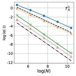
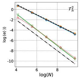
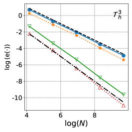
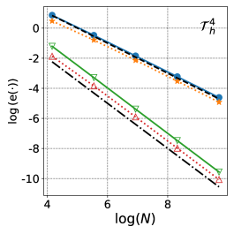
Figure 6.1: Test 6.1. Error curves of the virtual element scheme for the Brinkman equations using different meshes. Here, we set the parameters $\mathbb{K}=\mathbb{I}$, and $\nu=1$.

$\boldsymbol{u}_{1,h}$

$\boldsymbol{u}_{2,h}$

$|\boldsymbol{u}_{h}|$

Figure 6.2: Test 6.1. Scalar components of the computed velocity $\boldsymbol{u}_{i,h},i=1,2$ in different meshes together with the corresponding field $\boldsymbol{u}_{h}$.

$p_{h}$

$p_{h}$

$p_{h}$

Figure 6.3: Test 6.1. Comparison between the computed pressure $p_{h}$ on different polygonal meshes.

6.2 Robustness with respect to $\nu$

In this section we aim to test the robustness of the scheme with respect to the viscosity. More precisely, we observe the error behavior when $\nu$ becomes small. For simplicity, the exact solutions are the ones given in section 6.1, and we take $\mathcal{T}=\mathcal{T}_{3,h}$ (Voronoi mesh).

We consider a given viscosity $\nu=10^{-3j},\,j=1,2,3,4,$ and $\mathbb{K}=\mathbb{I}$. The computed errors and experimental rates of convergence are given in Tables 6.3-6.4. We observe small variations in the computed errors between taking $\nu=10^{-3}$ and the rest, that do not affect the convergence rate. This can also be said about the present results and the ones given in Section 6.1 for $\mathcal{T}_{3,h}$. The pattern is repeated for the scheme orders $k=2,3$, confirming the theoretical robustness with respect to the viscosity predicted in Section 5.

Table 6.3: Example 6.2. Error history with respect to different values of $\nu$ on the unit square domain for $\boldsymbol{u}_{h}$ and $p_{h}$. Here, we consider $k=2$ as the scheme order.

$\nu$	N	$h$	$\mathrm{e}(\boldsymbol{u})$	$r(\boldsymbol{u})$	$\mathrm{e}(p)$	$r(p)$	$\|\nabla\cdot\boldsymbol{u}_{h}\|_{0,\Omega}$
$10^{-3}$	64	0.162	2.19e+00	$\star$	9.48e-02	$\star$	7.04e-03
	256	0.089	4.95e-01	2.14	3.02e-02	1.65	8.14e-04
	1024	0.046	1.28e-01	1.96	6.72e-03	2.17	1.10e-04
	4096	0.021	3.03e-02	2.08	1.62e-03	2.05	1.92e-05
	16384	0.011	7.54e-03	2.00	3.68e-04	2.14	1.10e-06
$10^{-6}$	64	0.162	2.37e+00	$\star$	9.40e-02	$\star$	7.04e-03
	256	0.089	5.61e-01	2.08	3.00e-02	1.65	8.14e-04
	1024	0.046	1.49e-01	1.91	6.66e-03	2.17	1.10e-04
	4096	0.021	3.37e-02	2.14	1.61e-03	2.05	1.92e-05
	16384	0.011	8.27e-03	2.03	3.65e-04	2.14	1.10e-06
$10^{-9}$	64	0.162	2.37e+00	$\star$	9.40e-02	$\star$	7.04e-03
	256	0.089	5.61e-01	2.08	3.00e-02	1.65	8.14e-04
	1024	0.046	1.49e-01	1.91	6.66e-03	2.17	1.10e-04
	4096	0.021	3.39e-02	2.14	1.61e-03	2.05	1.92e-05
	16384	0.011	8.44e-03	2.01	3.65e-04	2.14	1.10e-06
$10^{-12}$	64	0.162	2.37e+00	$\star$	9.40e-02	$\star$	7.04e-03
	256	0.089	5.61e-01	2.08	3.00e-02	1.65	8.14e-04
	1024	0.046	1.49e-01	1.91	6.66e-03	2.17	1.10e-04
	4096	0.021	3.39e-02	2.14	1.61e-03	2.05	1.92e-05
	16384	0.011	8.44e-03	2.01	3.65e-04	2.14	1.10e-06

Table 6.4: Example 6.2. Error history with respect to different values of $\nu$ on the unit square domain for $\boldsymbol{u}_{h}$ and $p_{h}$. Here, we consider $k=3$ as the scheme order.

$\nu$	N	$h$	$\mathrm{e}(\boldsymbol{u})$	$r(\boldsymbol{u})$	$\mathrm{e}(p)$	$r(p)$	$\|\nabla\cdot\boldsymbol{u}_{h}\|_{0,\Omega}$
$10^{-3}$	64	0.162	2.74e-01	$\star$	1.15e-02	$\star$	1.02e-04
	256	0.089	2.96e-02	3.21	1.44e-03	3.00	7.42e-06
	1024	0.046	4.06e-03	2.87	1.59e-04	3.18	1.75e-06
	4096	0.021	5.01e-04	3.02	1.52e-05	3.38	6.56e-07
	16384	0.011	6.54e-05	2.94	1.66e-06	3.20	2.32e-07
$10^{-6}$	64	0.162	3.47e-01	$\star$	1.14e-02	$\star$	1.02e-04
	256	0.089	4.45e-02	2.96	1.43e-03	3.00	7.42e-06
	1024	0.046	5.96e-03	2.90	1.58e-04	3.18	1.75e-06
	4096	0.021	6.80e-04	3.13	1.51e-05	3.38	6.56e-07
	16384	0.011	8.09e-05	3.07	1.65e-06	3.20	2.32e-07
$10^{-9}$	64	0.162	3.47e-01	$\star$	1.14e-02	$\star$	1.02e-04
	256	0.089	4.46e-02	2.96	1.43e-03	3.00	7.42e-06
	1024	0.046	6.00e-03	2.89	1.58e-04	3.18	1.75e-06
	4096	0.021	6.93e-04	3.11	1.51e-05	3.38	6.56e-07
	16384	0.011	8.68e-05	3.00	1.65e-06	3.20	2.32e-07
$10^{-12}$	64	0.162	3.47e-01	$\star$	1.14e-02	$\star$	1.02e-04
	256	0.089	4.46e-02	2.96	1.43e-03	3.00	7.42e-06
	1024	0.046	6.00e-03	2.89	1.58e-04	3.18	1.75e-06
	4096	0.021	6.93e-04	3.11	1.51e-05	3.38	6.56e-07
	16384	0.011	8.68e-05	3.00	1.65e-06	3.20	2.32e-07

6.3 Applications with several boundary conditions

This experiment aims to test the behavior of our method in applications where several geometric conditions are assumed. Let $\boldsymbol{g}_{1}$ and $\boldsymbol{g}_{2}$ be two vector fields such that

$$\boldsymbol{u}\cdot\boldsymbol{n}=\boldsymbol{g}_{1}\cdot\boldsymbol{n},\qquad(\boldsymbol{\varepsilon}(\boldsymbol{u}))\boldsymbol{n}\cdot\boldsymbol{t}=\boldsymbol{g}_{2}\cdot\boldsymbol{t},\quad\text{ on }\Gamma_{N}.$$

Then, the discrete right-hand sides forms with additional Nitsche terms are given as follow (cf. Section 3.1).

$$\widetilde{F}_{h}(\boldsymbol{v}_{h}) :=F_{h}(\boldsymbol{v}_{h})+\gamma_{N}\sum_{e\in\mathcal{E}_{h}^{N}}\int_{e}h_{e}^{-1}(\boldsymbol{g}_{1}\cdot\boldsymbol{n})(\boldsymbol{v}_{h}\cdot\boldsymbol{n})\,\mathrm{d}s-\sum_{e\in\mathcal{E}_{h}^{N}}\int_{e}(\boldsymbol{n}^{t}(\nu\boldsymbol{\varepsilon}({\Pi^{\boldsymbol{\varepsilon},k}_{K_{e}}}\boldsymbol{v}_{h})\boldsymbol{n}))(\boldsymbol{g}_{1}\cdot\boldsymbol{n})\,\mathrm{d}s$$

$$\hskip 56.9055pt+\sum_{e\in\mathcal{E}_{h}^{N}}\int_{e}(\boldsymbol{g}_{2}\cdot\boldsymbol{t})(\boldsymbol{v}_{h}\cdot\boldsymbol{t})\,\mathrm{d}s$$

$$\widetilde{G}(q_{h}):=G(q_{h})+\sum_{e\in\mathcal{E}_{h}^{N}}\int_{e}\boldsymbol{g}_{1}\cdot(q_{h}\boldsymbol{n})\,\mathrm{d}s.$$

We divide the test in three cases, that we detail below.

6.3.1 Flow past cylinder

We first focuse on the simulation of a cross-flow around a cylinder between two paralel plates. This phenomena can be characterized in a 2D model, for which we take $R=0.05$ as the radius of the cylinder, and the length and height of the channel are given by $L=0.82$ and $H=0.41$, respectively. The resulting domain is of the form

$$\Omega:=(0,L)\times(0,H)\backslash D_{R}(x_{c},y_{c}),$$

where $D_{R}$ is the disk of radius $R$ and centered at $(x_{c},y_{c})=(0.2,0.2)$. We divide the boundaries as $\partial\Omega:=\Gamma_{\text{in}}\cup\Gamma_{\text{wall}}\cup\Gamma_{\text{circ}}\cup\Gamma_{\text{out}}$, corresponding to the inlet, walls, inner circle and outlet boundary, respectively. Each of these subdomains have the following data.

$$\boldsymbol{u}=\boldsymbol{0},\quad\text{ on }\Gamma_{w}\cup\Gamma_{\text{circ}},$$

$$\boldsymbol{u}\cdot\boldsymbol{n}=\boldsymbol{g}_{1}\cdot\boldsymbol{n},\quad(\nu\boldsymbol{\varepsilon}(\boldsymbol{u}))\boldsymbol{n}\cdot\boldsymbol{t}=\boldsymbol{g}_{1}\cdot\boldsymbol{t},\quad\text{ with }\boldsymbol{g}_{1}(x,y)=\left(\frac{6u_{\max}y(H-y)}{H^{2}},0\right)^{\texttt{t}},\quad\text{ on }\Gamma_{\text{in}},$$

$$(\nu\boldsymbol{\varepsilon}(\boldsymbol{u})-p\mathbb{I})\boldsymbol{n}=\boldsymbol{0},\quad\text{on }\Gamma_{\text{out}},$$

with $u_{\max}=2$. The viscosity is taken to be $\nu=1$. Note that $\boldsymbol{g}_{1}$ corresponds to a Poiseuille flow and the condition over $\Gamma_{\text{out}}$ is a free flow boundary condition, which is beyond the scope of the proposed theory.

We have depicted the computed velocity data in Figure 6.4. Here, we observe that the boundary conditions are applied correctly, having no-slip around the inner circle and the walls. Also, by comparing the plots of $\boldsymbol{u}_{1,h}$ and $\boldsymbol{u}_{2,h}$ in the outflow we observe that is similar to that of Stokes and Navier-stokes on a channel that ends at $\Gamma_{\text{out}}$. To observe the behavior at the inlet, we have also plotted the velocity profiles in Figure 6.5. Here, we observe that the parabolic and zero-tangential stress profiles are properly imposed. We finish this part of the experiment showing the surface plot of the pressure drop on two different meshes in Figure 6.6.

$\boldsymbol{u}_{1,h}$

$\boldsymbol{u}_{2,h}$

$|\boldsymbol{u}_{h}|$

$|\boldsymbol{u}_{h}|$

Figure 6.4: Test 6.3.1. Computed scalar components of the velocity field (top) along with the corresponding velocity field and streamlines (bottom) in the cross-flow model.

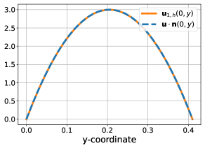
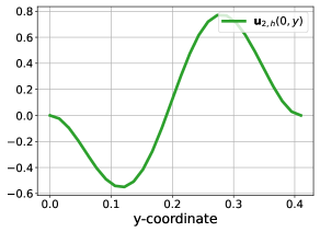
Figure 6.5: Test 6.3.1. Plots of the resulting computed inlet velocity components weakly imposed at $\Gamma_{\text{in}}$. The behavior of $\boldsymbol{u}_{2,h}$ results from imposing $(\nu\boldsymbol{\varepsilon}(\boldsymbol{u}))\boldsymbol{n}\cdot\boldsymbol{t}=\boldsymbol{g}_{1}\cdot\boldsymbol{t}$.

$p_{h},\;\mathcal{T}_{1,h}$

$p_{h},\;\mathcal{T}_{3,h}$

Figure 6.6: Test 6.3.1. Comparison between computed pressures in the cross-flow model using $\mathcal{T}_{1,h}$ and $\mathcal{T}_{3,h}$.

6.3.2 Flow into a backwards facing step

A classical benchmark test for Stokes, Navier-Stokes or Brinkman equations is the backward facing step. Let us consider $H:=1$ and a channel given by

$$\Omega:=(0,9H)\times(0,2H)\backslash\{(0,2H)\times(0,H)\},$$

where we have a backward facing step in $(2H,H)$. We consider as the inlet region the left boundary, where we weakly impose

$$\boldsymbol{u}\cdot\boldsymbol{n}=\boldsymbol{g}_{1}\cdot\boldsymbol{n},\quad(\nu\boldsymbol{\varepsilon}(\boldsymbol{u}))\boldsymbol{n}\cdot\boldsymbol{t}=\boldsymbol{g}_{1}\cdot\boldsymbol{t},\quad\text{with }\quad\boldsymbol{g}_{1}(x,y)=\left(u_{\max}-0.5(y-1.5H)^{2},0\right)^{\texttt{t}}.$$

As before, the inflow consist of a Poiseuille type flow, with $u_{\max}=0.125$. In the outlet (right boundary), we impose a zero stress boundary condition $(\nu\boldsymbol{\epsilon}(\boldsymbol{u})-p\mathbb{I})\boldsymbol{n}=\boldsymbol{0}$, and no-slip boundary conditions on the rest of $\partial\Omega$. The viscosity is taken to be $\nu=1$. The experiment was carried in two different Voronoi meshes: one with 4096 elements, and the other with 16384. The behavior for both meshes where similar, and we present the results with the coarsest mesh. The physical parameters were taken as $\mathbb{K}=\mathbb{I}$ and $\nu=1$. The approximated velocity field and pressure are presented in Figure 6.7. Here, we have some well-known phenomena that include singularities at the reentrant corner and recirculation zones. The negative pressure values is valid due to the incompressible formulation of the problem, which allows to write the variable $p$ in terms of the gauge pressure. To observe the weak imposition of the boundary conditions at the inlet, we depict the velocity components in Figure 6.8, where we have a parabolic behavior of the first velocity component together with the tangential stress provided by the Poiseuille flow.

$\boldsymbol{u}_{2,h}$

$|\boldsymbol{u}_{h}|$

$|\boldsymbol{u}_{h}|$

$p_{h}$

Figure 6.7: Test 6.3.2. Second velocity compoment (top) Velocity field streamlines (two in the middle) with pressure distribution (bottom), computed in a Voronoi mesh with 4096 elements.

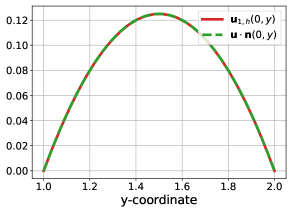
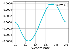
Figure 6.8: Test 6.3.2. Plots of the resulting computed inlet velocity components weakly imposed at the inlet for the flow into a backwards facing step. The behavior of $\boldsymbol{u}_{2,h}$ results from imposing $(\nu\boldsymbol{\varepsilon}(\boldsymbol{u}))\boldsymbol{n}\cdot\boldsymbol{t}=\boldsymbol{g}_{1}\cdot\boldsymbol{t}$.

6.3.3 The lid-driven cavity flow

We end this section by performing the classical lid-driven cavity test where we model the steady flow of an immiscible fluid in a box. We consider the unit square domain $\Omega=(0,1)^{2}$. The viscosity is taken to be $\nu=10^{-3}$. The test is initially done with $\mathbb{K}=\kappa\mathbb{I}$, with $\kappa=10^{8}$. We take $\Gamma_{N}=\emptyset$ and $\Gamma_{D}=\Gamma_{\text{wall}}\cup\Gamma_{\text{lid}}$, where $\Gamma_{\text{wall}}$ corresponds to the bottom, left and right boundarires, and $\Gamma_{\text{lid}}$ is the top boundary. We set $\boldsymbol{u}|_{\Gamma_{\text{lid}}}=(1,0)^{\texttt{t}}$ and $\boldsymbol{u}|_{\Gamma_{\text{wall}}}=\boldsymbol{0}$. We note that this type of boundary condition is also not covered by the theory.

The approximate velocities and pressure (displayed in Figure 6.9) remain stable and corner singularities are clearly observed. Moreover, to assess the robustness of the method with respect to the choice of $\mathbb{K}$ , we run several tests varying $\mathbb{K}$ and keeping $\nu=10^{-3}$. Plots of the streamlines of each case are presented on Figure 6.10, where we confirm the stability of the approximation for each choice of $\mathbb{K}$.

$\boldsymbol{u}_{1,h}$

$\boldsymbol{u}_{2,h}$

$|\boldsymbol{u}_{h}|$

$p_{h}$

Figure 6.9: Test 6.3.3. Approximated velocity components and computed pressure on a Voronoi mesh for the lid-driven cavity test.

$\mathbb{K}^{-1}=10^{-8}\mathbb{I}$

$\mathbb{K}^{-1}=10\mathbb{I}$

$\mathbb{K}^{-1}=10^{2}\mathbb{I}$

$\mathbb{K}^{-1}=10^{8}\mathbb{I}$

Figure 6.10: Test 6.3.3. Comparison of the velocity streamlines obtained for several values of $\mathbb{K}$ for the lid-driven cavity test.

References

• (1) V. Anaya, D. Mora, R. Oyarzúa, and R. Ruiz-Baier, A priori and a posteriori error analysis of a mixed scheme for the Brinkman problem, Numer. Math., 133 (2016), pp. 781–817.
• (2) V. Anaya, D. Mora, and R. Ruiz-Baier, Pure vorticity formulation and Galerkin discretization for the Brinkman equations, IMA J. Numer. Anal., 37 (2017), pp. 2020–2041.
• (3) P. F. Antonietti, L. Beirão da Veiga, and G. Manzini, eds., The virtual element method and its applications, vol. 31 of SEMA SIMAI Springer Series, Springer, Cham, [2022] ©2022.
• (4) P. F. Antonietti, L. Beirão da Veiga, D. Mora, and M. Verani, A stream virtual element formulation of the Stokes problem on polygonal meshes, SIAM J. Numer. Anal., 52 (2014), pp. 386–404.
• (5) P. F. Antonietti, C. Facciolà, P. Houston, I. Mazzieri, G. Pennesi, and M. Verani, High-order discontinuous Galerkin methods on polyhedral grids for geophysical applications: seismic wave propagation and fractured reservoir simulations, in Polyhedral methods in geosciences, vol. 27 of SEMA SIMAI Springer Ser., Springer, Cham, [2021] ©2021, pp. 159–225.
• (6) H. J. Barbosa and T. J. Hughes, The finite element method with lagrange multipliers on the boundary: circumventing the babuška-brezzi condition, Computer Methods in Applied Mechanics and Engineering, 85 (1991), pp. 109–128.
• (7) L. Beirão da Veiga, F. Brezzi, L. D. Marini, and A. Russo, The virtual element method, Acta Numer., 32 (2023), pp. 123–202.
• (8) L. Beirão da Veiga, K. Lipnikov, and G. Manzini, The mimetic finite difference method for elliptic problems, vol. 11 of MS&A. Modeling, Simulation and Applications, Springer, Cham, 2014.
• (9) L. Beirão da Veiga, C. Lovadina, and G. Vacca, Divergence free virtual elements for the Stokes problem on polygonal meshes, ESAIM Math. Model. Numer. Anal., 51 (2017), pp. 509–535.
• (10) L. Beirão da Veiga, C. Lovadina, and G. Vacca, Virtual elements for the Navier-Stokes problem on polygonal meshes, SIAM J. Numer. Anal., 56 (2018), pp. 1210–1242.
• (11) L. Beirão da Veiga, D. Mora, and G. Vacca, The Stokes complex for virtual elements with application to Navier-Stokes flows, J. Sci. Comput., 81 (2019), pp. 990–1018.
• (12) L. Beirão da Veiga, F. Brezzi, A. Cangiani, G. Manzini, L. D. Marini, and A. Russo, Basic principles of virtual element methods, Mathematical Models and Methods in Applied Sciences, 23 (2013), pp. 199–214.
• (13) S. Bertoluzza, M. Pennacchio, and D. Prada, Weakly imposed dirichlet boundary conditions for 2d and 3d virtual elements, Computer Methods in Applied Mechanics and Engineering, 400 (2022), p. 115454.
• (14) D. Boffi, F. Brezzi, M. Fortin, et al., Mixed finite element methods and applications, vol. 44, Springer, 2013.
• (15) L. Botti, D. A. Di Pietro, and J. Droniou, A Hybrid High-Order discretisation of the Brinkman problem robust in the Darcy and Stokes limits, Comput. Methods Appl. Mech. Engrg., 341 (2018), pp. 278–310.
• (16) S. C. Brenner, The mathematical theory of finite element methods, Springer, 2008.
• (17) E. Cáceres and G. N. Gatica, A mixed virtual element method for the pseudostress-velocity formulation of the Stokes problem, IMA J. Numer. Anal., 37 (2017), pp. 296–331.
• (18) E. Cáceres, G. N. Gatica, and F. A. Sequeira, A mixed virtual element method for the Brinkman problem, Math. Models Methods Appl. Sci., 27 (2017), pp. 707–743.
• (19) A. Cangiani, E. H. Georgoulis, and P. Houston, $hp$-version discontinuous Galerkin methods on polygonal and polyhedral meshes, Math. Models Methods Appl. Sci., 24 (2014), pp. 2009–2041.
• (20) N. Carro, D. Mora, and J. Vellojin, A finite element model for concentration polarization and osmotic effects in a membrane channel, Internat. J. Numer. Methods Fluids, 96 (2024), pp. 601–625.
• (21) F. Chouly and P. Hild, A nitsche-based method for unilateral contact problems: numerical analysis, SIAM Journal on Numerical Analysis, 51 (2013), pp. 1295–1307.
• (22) F. Chouly, R. Mlika, and Y. Renard, An unbiased nitsche’s approximation of the frictional contact between two elastic structures, Numerische Mathematik, 139 (2018), pp. 593–631.
• (23) A. Dedner and A. Hodson, A framework for implementing general virtual element spaces, SIAM Journal on Scientific Computing, 46 (2024), pp. B229–B253.
• (24) A. Dedner, R. Klöfkorn, M. Nolte, and M. Ohlberger, A generic interface for parallel and adaptive discretization schemes: abstraction principles and the dune-fem module, Computing, 90 (2010), pp. 165–196.
• (25) D. A. Di Pietro and J. Droniou, The hybrid high-order method for polytopal meshes, vol. 19 of MS&A. Modeling, Simulation and Applications, Springer, Cham, [2020] ©2020. Design, analysis, and applications.
• (26) D. A. Di Pietro and J. Droniou, A polytopal method for the Brinkman problem robust in all regimes, Comput. Methods Appl. Mech. Engrg., 409 (2023), pp. Paper No. 115981, 23.
• (27) D. A. Di Pietro and A. Ern, A hybrid high-order locking-free method for linear elasticity on general meshes, Comput. Methods Appl. Mech. Engrg., 283 (2015), pp. 1–21.
• (28) G. N. Gatica, M. Munar, and F. A. Sequeira, A mixed virtual element method for a nonlinear Brinkman model of porous media flow, Calcolo, 55 (2018), pp. Paper No. 21, 36.
• (29) G. N. Gatica and F. A. Sequeira, An ${\rm L}^{p}$ spaces-based mixed virtual element method for the two-dimensional Navier-Stokes equations, Math. Models Methods Appl. Sci., 31 (2021), pp. 2937–2977.
• (30) L. F. Gatica and F. A. Sequeira, A priori and a posteriori error analyses of an HDG method for the Brinkman problem, Comput. Math. Appl., 75 (2018), pp. 1191–1212.
• (31) C. Geuzaine and J.-F. Remacle, Gmsh: A 3-d finite element mesh generator with built-in pre-and post-processing facilities, International journal for numerical methods in engineering, 79 (2009), pp. 1309–1331.
• (32) I. Gjerde and L. Scott, Nitsche’s method for navier–stokes equations with slip boundary conditions, Mathematics of Computation, 91 (2022), pp. 597–622.
• (33) P. Hansbo, Nitsche’s method for interface problems in computa-tional mechanics, GAMM-Mitteilungen, 28 (2005), pp. 183–206.
• (34) X. Huang and F. Wang, Analysis of divergence free conforming virtual elements for the Brinkman problem, Math. Models Methods Appl. Sci., 33 (2023), pp. 1245–1280.
• (35) M. Juntunen and R. Stenberg, Nitsche’s method for general boundary conditions, Mathematics of computation, 78 (2009), pp. 1353–1374.
• (36) A. Massing, B. Schott, and W. A. Wall, A stabilized Nitsche cut finite element method for the Oseen problem, Comput. Methods Appl. Mech. Engrg., 328 (2018), pp. 262–300.
• (37) S. Meddahi and R. Ruiz-Baier, A new DG method for a pure-stress formulation of the Brinkman problem with strong symmetry, Netw. Heterog. Media, 17 (2022), pp. 893–916.
• (38) D. Mora, C. Reales, and A. Silgado, A $C^{1}$-virtual element method of high order for the Brinkman equations in stream function formulation with pressure recovery, IMA J. Numer. Anal., 42 (2022), pp. 3632–3674.
• (39) J. Nitsche, Über ein variationsprinzip zur lösung von dirichlet-problemen bei verwendung von teilräumen, die keinen randbedingungen unterworfen sind, in Abhandlungen aus dem mathematischen Seminar der Universität Hamburg, vol. 36, Springer, 1971, pp. 9–15.
• (40) N. Schlömer, pygmsh: a Python frontend for Gmsh, Zenodo, (2021).
• (41) C. Talischi, G. H. Paulino, A. Pereira, and I. F. Menezes, Polymesher: a general-purpose mesh generator for polygonal elements written in Matlab, Structural and Multidisciplinary Optimization, 45 (2012), pp. 309–328.
• (42) J. M. Urquiza, A. Garon, and M.-I. Farinas, Weak imposition of the slip boundary condition on curved boundaries for stokes flow, Journal of Computational Physics, 256 (2014), pp. 748–767.
• (43) G. Vacca, An $H^{1}$-conforming virtual element for Darcy and Brinkman equations, Mathematical Models and Methods in Applied Sciences, 28 (2018), pp. 159–194.
• (44) P. Virtanen, R. Gommers, T. E. Oliphant, M. Haberland, T. Reddy, D. Cournapeau, E. Burovski, P. Peterson, W. Weckesser, J. Bright, S. J. van der Walt, M. Brett, J. Wilson, K. J. Millman, N. Mayorov, A. R. J. Nelson, E. Jones, R. Kern, E. Larson, C. J. Carey, İ. Polat, Y. Feng, E. W. Moore, J. VanderPlas, D. Laxalde, J. Perktold, R. Cimrman, I. Henriksen, E. A. Quintero, C. R. Harris, A. M. Archibald, A. H. Ribeiro, F. Pedregosa, P. van Mulbregt, and SciPy 1.0 Contributors, SciPy 1.0: Fundamental Algorithms for Scientific Computing in Python, Nature Methods, 17 (2020), pp. 261–272.
• (45) L. Zhao, E. Chung, and M. F. Lam, A new staggered DG method for the Brinkman problem robust in the Darcy and Stokes limits, Comput. Methods Appl. Mech. Engrg., 364 (2020), pp. 112986, 18.