Bifurcation analysis of figure-eight choreography in the three-body problem based on crystallographic point groups

Abstract

We report on the bifurcation analysis of figure-eight choreography by irreducible real orthogonal representations of its symmetry groups based on variational principle of the action. There are four types of bifurcation solutions in the sequence of the bifurcation cascade: (i) the trivial type represented by trivial representation, (ii) the two-fold type by non-trivial one-dimensional representation, (iii) the three-fold and (iv) the six-fold types by two-dimensional irreducible representations. As numerical examples, we present four new bifurcation solutions: non-symmetric choreographic solution of the two-fold type, non-planar solution of the two-fold type, $y$-axis symmetric solution of the three-fold type, and non-symmetric solution of the six-fold type.

Keywords: irreducible representation, real orthogonal representation, symmetry

1 Introduction

The figure-eight choreography in the three-body problem is a motion of three equal masses, chasing each other in the common figure-eight shaped orbit [1, 2]. For inhomogeneous interaction potential, the shape of the orbit varies as a function of the period of the motion and it bifurcates [3, 4, 5, 6]. For homogeneous interaction potential, it remains similar independent of the period, however, bifurcations occur by the power of homogeneous potential or one of the masses of the bodies as a parameter [6, 7, 8].

In this paper, we analyze the bifurcation of the figure-eight choreography based on crystallographic point group and the variational principle of the action [9]. In section 2, a necessary condition for bifurcation are shown and a representation of bifurcation solutions by the Lyapunov-Schmidt reduction is proposed. In section 3, a theorem on the representation is proved, then a corollary on symmetries of bifurcation solution is derived. In section 4, another corollary on symmetries of the Lyapunov-Schmidt reduced action is derived. From the corollaries, it is shown that four types of bifurcation are possible. In section 5, numerically calculated bifurcation solutions, including four new solutions, are shown. Section 6 is summary and discussions.

2 Necessary condition and representation for bifurcation

We consider a periodic solution $q(t)=q(t+T)$ with the period $T$ of the Euler-Lagrange equations

$$\frac{d}{dt}\frac{\partial L}{\partial\dot{q}}=\frac{\partial L}{\partial q}$$ (1)

for the Lagrangian of the equal mass three-body problem:

$$L=\frac{1}{2}\dot{q}^{2}-U,\;U=\sum_{i>j}u(|\bi{r}_{i}-\bi{r}_{j}|),$$ (2)

where $\bi{r}_{i}=(x_{i},y_{i},z_{i})$, $i=1,2,3$ are the position vectors of body $i$ and

$$q=(q_{1},q_{2},\ldots,q_{N})=(x_{1},y_{1},z_{1},x_{2},y_{2},z_{2},x_{3},y_{3},z_{3}),$$ (3)

with $N=9$. We use matrix notation, however, we do not distinguish column and row vectors strictly if it is obvious from the context.

2.1 Necessary condition for bifurcation

Suppose a periodic solution $q$ depends on a parameter $\xi$, such as the period $T$ or the order of homogeneous potential and bifurcates into $q^{(b)}$ at $\xi=\xi^{(b)}$. Since both $q$ and $q^{(b)}$ are solutions of (1) with (2), their difference

$$\Delta q=q^{(b)}-q$$ (4)

satisfies a relation made of the Hessian of the Lagrangian

$$\frac{d^{2}}{dt^{2}}\Delta q=\left.\frac{\partial L}{\partial q}\right|_{q+\Delta q}-\frac{\partial L}{\partial q}=\left(\frac{\partial}{\partial q}\frac{\partial L}{\partial q}\right)\Delta q+\Or\left(|\Delta q|^{2}\right).$$ (5)

We thus define an $N\times N$ matrix operator,

$$H(q)=-\frac{d^{2}}{dt^{2}}+\frac{\partial^{2}}{\partial q^{2}}L(q,\dot{q}),$$ (6)

and consider an eigenvalue problem of $H(q)$

$$H(q)v=\alpha v,$$ (7)

where $v$ is a column vector of length $N$ and $\alpha$ an eigenvalue. Since $H(q)$ is real symmetric, both $\alpha$ and $v$ are real.

For $\xi\to\xi^{(b)}$, by the relation (5), there exist eigenvalues

$$\alpha\to 0$$ (8)

with

$$\Delta q\to v.$$ (9)

2.2 Representation of bifurcation

In the vicinity of the bifurcation point $\xi^{(b)}$, we represent the bifurcation solution as

$$q^{(b)}=q+h(\phi r+\psi\epsilon).$$ (10)

Here,

$$\phi=(\phi_{1},\phi_{2},\ldots,\phi_{d})$$ (11)

is an $N\times d$ matrix composed of orthonormal eigenfunctions of $H(q)$

$$H(q)\phi_{i}=\kappa_{i}\phi_{i},\;\int_{0}^{T}dt\phi_{i}\phi_{j}=\delta_{ij},$$ (12)

for eigenvalues $\kappa_{i}$ going to zero for $\xi\to\xi^{(b)}$, and

$$\psi=(\psi_{1},\psi_{2},\ldots)$$ (13)

is the orthonormal eigenfunctions for the other, non zero, eigenvalues $\lambda_{i}$,

$$H(q)\psi_{i}=\lambda_{i}\psi_{i},\;\int_{0}^{T}dt\psi_{i}\psi_{j}=\delta_{ij},$$ (14)

where $\delta_{ij}$ is Kronecker delta. The coefficients $r$ and $\epsilon$ are the column vectors

$$r={}^{t}(r_{1},r_{2},\ldots,r_{d}),\;\epsilon={}^{t}(\epsilon_{1},\epsilon_{2},\ldots),$$ (15)

with $r_{i}\in\mathbb{R}$ and $\epsilon_{i}\in\mathbb{R}$, where ^t denotes transpose. A factor $h=1$ is introduced to count the order $\Delta q$.

In this representation by $r$ and $\epsilon$, variational principle of action

$$\frac{\partial}{\partial r}S(q+h(\phi r+\psi\epsilon))=0,\;$$ (16)

$$\frac{\partial}{\partial\epsilon}S(q+h(\phi r+\psi\epsilon))=0,$$ (17)

is suitable for the Euler-Lagrange equation (1), where $S(f)$ is the action of periodic function $f(t+T)=f(t)$,

$$S(f)=\int_{0}^{T}L(f,\dot{f})dt.$$ (18)

A solution of (16) and (17) at $r\to 0$ for $\xi\to\xi^{(b)}$ corresponds to a bifurcation solution $q^{(b)}$ and that at $r=0$ the original solution $q$.

We introduce seven variation functions corresponding to infinitesimally small translation of time, translation, and infinitesimally small rotation,

$$\Phi_{1}=\dot{q},\;\Phi_{2}=(e_{x},e_{x},e_{x}),\;\Phi_{3}=(e_{y},e_{y},e_{y}),\;\Phi_{4}=(e_{z},e_{z},e_{z}),$$ (19)

$$\Phi_{5}=q\times e_{x},\;\Phi_{6}=q\times e_{y},\;\Phi_{7}=q\times e_{z},\;$$ (20)

where $e_{i}=(\delta_{xi},\delta_{yi},\delta_{zi})$, $q\times e_{i}=(\bi{r}_{1}\times e_{i},\bi{r}_{2}\times e_{i},\bi{r}_{3}\times e_{i})$, and $\times$ is outer product. These are eigenfunctions of $H(q)$ for zero eigenvalue,

$$H(q)\Phi_{i}=0,\;i=1,2,\ldots 7$$ (21)

and do not contribute to the variational principle (16), since for any $r$

$$\frac{\partial}{\partial r}S(q+\Phi_{i}r)=0.$$ (22)

Thus we exclude the seven eigenfunctions (19)–(20) from (11). Then in the simple case $\phi$ spans eigenspace of $d$ degenerate eigenvalues $\kappa_{1}=\kappa_{2}=\cdots=\kappa_{d}$.

The following methods, utilizing irreducible representation, the Lyapunov-Schmidt reduction are developed in the area of condensed matter physics, particle physics, etc. [10, 11, 12, 13, 14].

2.3 The Lyapunov-Schmidt reduction

Formally $\epsilon$ in the representation (10) is determined by expanding $S$ in (17) in powes of $h$,

$$S(q+h\delta q)=\sum_{k=1}^{\infty}\frac{h^{k}}{k!}S^{(k)}(q,\delta q),$$ (23)

where

$$S^{(k)}(q,\delta q)=\int_{0}^{T}dt\left(\delta q\frac{\partial}{\partial q}+\dot{\delta q}\frac{\partial}{\partial\dot{q}}\right)^{k}L,$$ (24)

is the $k$th variation of the action and $\delta q=\phi r+\psi\epsilon$. The first variation

$$S^{(1)}(q,\delta q)=\int_{0}^{T}dt\delta q\left(\frac{\partial L}{\partial q}-\frac{d}{dt}\frac{\partial L}{\partial\dot{q}}\right)$$ (25)

is zero since $q$ satisfies (1). The second variation is written by integral by parts as

$$S^{(2)}(q,\delta q)=\int_{0}^{T}dt\delta qH(q)\delta q=\sum_{i=1}^{d}\kappa_{i}r_{i}^{2}+\sum_{i}\lambda_{i}\epsilon_{i}^{2}$$ (26)

and for $k\geq 3$,

$$S^{(k)}(q,\delta q)=\int_{0}^{T}dt\left((\phi r+\psi\epsilon)\frac{\partial}{\partial q}\right)^{k}L.$$ (27)

Then (17)

$$\epsilon=\sum_{k=1}^{\infty}\frac{h^{k}}{(k+1)!\lambda}\int_{0}^{T}dt\left(\psi\frac{\partial}{\partial q}\right)\left((\phi r+\psi\epsilon)\frac{\partial}{\partial q}\right)^{k+1}L,$$ (28)

determines $\epsilon$ by the recursive substitution of $\epsilon$ from the left side to the right side as

$$\epsilon=h\epsilon^{(1)}+h^{2}\epsilon^{(2)}+\cdots,$$ (29)

$$\epsilon^{(1)}=-\frac{1}{2\lambda}\int_{0}^{T}dt(\psi\frac{\partial}{\partial q})(\phi r\frac{\partial}{\partial q})^{2}L,$$ (30)

$$\epsilon^{(2)}=-\frac{1}{6\lambda}\int_{0}^{T}dt\left((\psi\frac{\partial}{\partial q})(\phi r\frac{\partial}{\partial q})^{3}+6(\psi\frac{\partial}{\partial q})(\phi r\frac{\partial}{\partial q})(\psi\epsilon^{(1)}\frac{\partial}{\partial q})\right)L,$$ (31)

and so on, where

$$(\lambda)_{ij}=\delta_{ij}\lambda_{i}.$$ (32)

This procedure, known as the Lyapunov-Schmidt reduction, leaves $r$, and determines $\epsilon$ as a function of $r$, $\epsilon(r)$. Note that from (30) $\epsilon^{(1)}(\alpha r)=\alpha^{2}\epsilon^{(1)}(r)$, and then from (31), $\epsilon^{(2)}(\alpha r)=\alpha^{3}\epsilon^{(2)}(r)$, and by induction, $\epsilon^{(k)}(r)$ is homogeneous function of $r$,

$$\epsilon^{(k)}(\alpha r)=\alpha^{k+1}\epsilon^{(k)}(r),\;k=1,2,\ldots,\;\alpha\in\mathbb{R}.$$ (33)

Consequently, by the $\epsilon(r)$, the bifurcation solution (10) is represented by $r$,

$$q^{(b)}(r;q)=q+h(\phi r+\psi\epsilon(r)).$$ (34)

Thus, its action

$$S(r)=S(q^{(b)}(r;q)),$$ (35)

and the variational principle (16) and (17)

$$\frac{\partial}{\partial r}S(r)=0,$$ (36)

are also reduced into a $d$-dimensional space of $r$.

3 Symmetries of bifurcation solutions

We denote a symmetry group of a periodic function $f$ as

$$G(f)=\{g|gf=f\}.$$ (37)

If matrix $H(q)$ commutes with all $g\in G(q)$,

$$gH(q)=H(q)g,$$ (38)

the operation by $g\in G(q)$ to eigenfunction $\phi r$ of $H(q)$ is given by a $d$-dimensional representation $D(g)$, a $d\times d$ real orthogonal matrix, of $g$ as

$$g\phi r=\phi D(g)r,$$ (39)

since $\phi$ is real and orthonormal. Thus, $G(\phi r)$, a group of symmetries for $\phi r$, is written without $\phi$

$$G(r;q)=\{g|g\in G(q),D(g)r=r\}.$$ (40)

Further,

Theorem 1

If all $g\in G(q)$ commute with $H(q)$, the bifurcation solution $q^{(b)}(r;q)$ defined by (34) satisfies

$$gq^{(b)}(r;q)=q^{(b)}(D(g)r;q),$$ (41)

where $D(g)$ is a real orthogonal representation of $g$ in $\phi$, that is, $g\phi r=\phi D(g)r$.

Proof. Multiplying $\psi$ from the left, then operating $g$ in the both side of (28), we obtain

$$\psi D\epsilon=-\sum_{k>0}\frac{h^{k}}{(k+1)!\lambda}\psi\int_{0}^{T}dt\left(\psi\frac{\partial}{\partial q}\right)\left((\phi D(g)r+\psi D\epsilon)\frac{\partial}{\partial q}\right)^{k+1}L,$$ (42)

since $gL=L$ and $D\lambda^{-1}{}^{t}D=\lambda^{-1}$, where $D$ is the representation of $g$ in $\psi$. Then multiplying ${}^{t}\psi$ from the left in the both side and integrating by $t$ from $0$ to $T$,

$$D\epsilon=-\sum_{k>0}\frac{h^{k}}{(k+1)!\lambda}\int_{0}^{T}dt\left(\psi\frac{\partial}{\partial q}\right)\left((\phi D(g)r+\psi D\epsilon)\frac{\partial}{\partial q}\right)^{k+1}L.$$ (43)

Here (43) is obtained by replacing $r$ and $\epsilon$ by $D(g)r$ and $D\epsilon$ in (28), respectively. (28) determines $\epsilon$ from $r$, then (43) determines $D\epsilon$ from $D(q)r$. Thus $D\epsilon(r)=\epsilon(D(g)r)$. Since, for $g\in G(q)$, $gq^{(b)}(r;q)=g(q+h\phi r+\psi\epsilon(r))=q+h(\phi D(g)r+\psi D\epsilon(r))=q+h(\phi D(g)r+\epsilon(D(g)r))=q^{(b)}(D(g)r;q).$ □

Corollary 1

If all $g\in G(q)$ commute with $H(q)$, the bifurcation solution $q^{(b)}(r;q)$ is invariant under $g\in G(r;q)$, $gq^{(b)}(r;q)=q^{(b)}(r;q)$, or $G\left(q^{(b)}(r;q)\right)=G(r;q)$.

Therefore, the representations of $G(q)$ determine the symmetry of the bifurcation solution $q^{(b)}(r;q)$ independent of $H(q)$, if all $g\in G(q)$ commute with $H(q)$.

3.1 Symmetries of the figure-eight choreography

For the figure-eight choreography $q$, the $G(q)$ is generated by the four operators, choreographic shift ${\cal C}$,

$${\cal C}q(t)=\sigma q(t-T/3),\\$$ (44)

space and time inversion ${\cal S}$,

$${\cal S}q(t)=-\tau q(-t),\\$$ (45)

$x$-inversion with time shift ${\cal M}$,

$${\cal M}q(t)=\mu_{x}q(t-T/2),\\$$ (46)

and inversion of $z$ coordinate $\mu=\mu_{z}$, where $\sigma$ is cyclic permutation of bodies,

$$\sigma q=\sigma(\bi{r}_{1},\bi{r}_{2},\bi{r}_{3})=(\bi{r}_{2},\bi{r}_{3},\bi{r}_{1}),$$ (47)

$\tau$ exchange of body 1 and 2,

$$\tau q=\tau(\bi{r}_{1},\bi{r}_{2},\bi{r}_{3})=(\bi{r}_{2},\bi{r}_{1},\bi{r}_{3}),$$ (48)

$\mu_{j}$ inversion of $j=x,y,z$ coordinate,

$$\mu_{j}q=(\mu_{j}\bi{r}_{1},\mu_{j}\bi{r}_{2},\mu_{j}\bi{r}_{3}),\;\mu_{j}\bi{r}_{i}=(s_{xj}x_{i},s_{yj}y_{i},s_{zj}z_{i}),\;s_{cj}=1-2\delta_{cj},$$ (49)

and $\bi{r}_{3}=0$ at $t=0$ is assumed [2, 10, 9, 15]. Since

$${\cal C}^{3}={\cal S}^{2}={\cal M}^{2}=\mu^{2}=1,\;{\cal CS}={\cal SC}^{-1}$$ (50)

and

$${\cal CM}={\cal MC},\;{\cal C}\mu=\mu{\cal C},\;{\cal SM}={\cal MS},\;{\cal S}\mu=\mu{\cal S},\;{\cal M}\mu=\mu{\cal M},$$ (51)

the group $G(q)$ is isomorphic to a crystallographic point group $D_{6h}$ or a direct product of abstract groups $D_{6}\times C_{2}$ where $C_{n}$ and $D_{n}$ are the cyclic and the dihedral group, respectively [18]. Hereafter, we denote generators of the group by curly parenthesis following the Schoenflies notation of isomorphic group, then

$$G(q)=D_{6h}\{{\cal C},{\cal S},{\cal M},\mu\}.$$ (52)

It is verified that the operators $\mathcal{C}$, $\mathcal{S}$, $\mathcal{M}$ and $\mu$ commute with $H(q)$. Therefore, the symmetry group $G(r;q)$ for bifurcation solution $q^{(b)}(r;q)$ from figure-eight choreography $q$ is a real orthogonal representations of $D_{6h}\{{\cal C},{\cal S},{\cal M},\mu\}$ by the corollary 1.

3.2 Symmetries of the bifurcation solutions from figure-eight choreography

Table 1: Symmetries of bifurcation solution $G(r;q)$ for $D_{6h}\{{\cal CM},{\cal S},\mu\}$.

• $\{D({\cal CM}),D({\cal S}),D(\mu)\}$	$G(r;q)$
  $C_{1}\{+1,+1,+1\}$	$D_{6h}\{{\cal CM,S},\mu\}$		P
  $C_{2}\{+1,-1,+1\}$	$C_{6h}\{{\cal CM},\mu\}$		P
  $C_{2}\{-1,+1,+1\}$	$D_{6}\{\mu{\cal C},{\cal S}\}$		P
  $C_{2}\{-1,-1,+1\}$	$D_{6}\{\mu{\cal C},{\cal SM}\}$		P
  $C_{2}\{+1,+1,-1\}$	$D_{6}\{{\cal CM,S}\}$		I
  $C_{2}\{+1,-1,-1\}$	$D_{6}\{{\cal CM},\mu{\cal S}\}$		N
  $C_{2}\{-1,+1,-1\}$	$D_{6}\{\mu{\cal CM},{\cal S}\}$		I
  $C_{2}\{-1,-1,-1\}$	$D_{6}\{\mu{\cal CM},\mu{\cal S}\}$		N
  $D_{3}\{C(3),F,+E\}$	$\left\{\begin{array}[]{l}D_{2h}\{\mathcal{C}^{n-1}\mathcal{S},\mathcal{M},\mu\}\\ D_{2}\{\mathcal{M},\mu\}\end{array}\right.$	$\begin{array}[]{l}\displaystyle(\theta=\theta_{2n+1})\\ \mbox{(otherwise)}\end{array}$	P
  $D_{6}\{C(3),F,-E\}$	$\left\{\begin{array}[]{l}D_{2}\{\mu\mathcal{C}^{n+1}\mathcal{S},{\cal M}\}\\ D_{2}\{\mathcal{C}^{n-1}\mathcal{S},\mathcal{M}\}\\ C_{2}\{{\cal M}\}\\ \end{array}\right.$	$\begin{array}[]{l}(\theta=\theta_{2n})\\ (\theta=\theta_{2n+1})\\ (\mbox{otherwise})\end{array}$	I
  $D_{6}\{C(6),F,+E\}$	$\left\{\begin{array}[]{l}D_{2}\{\mathcal{C}^{-n}\mathcal{SM},\mu\}\\ D_{2}\{\mathcal{C}^{1-n}\mathcal{S},\mu\}\\ C_{2}\{\mu\}\end{array}\right.$	$\begin{array}[]{l}(\theta=\theta_{2n})\\ (\theta=\theta_{2n+1})\\ (\mbox{otherwise})\end{array}$	P
  $D_{6h}\{C(6),F,-E\}$	$\left\{\begin{array}[]{l}D_{2}\{\mathcal{C}^{-n}\mathcal{SM},\mu\mathcal{M}\}\\ D_{2}\{\mathcal{C}^{1-n}\mathcal{S},\mu\mathcal{M}\}\\ C_{2}\{\mu\mathcal{M}\}\end{array}\right.$	$\begin{array}[]{l}(\theta=\theta_{2n})\\ (\theta=\theta_{2n+1})\\ (\mbox{otherwise})\end{array}$	I

In table 1, symmetries of bifurcation solutions, $G(r;q)$, for the irreducible real orthogonal representation of $D_{6h}\{{\cal C},{\cal S},{\cal M},\mu\}$ are tabulated, where $D_{nh}=D_{n}\times C_{2}$, $C_{nh}=C_{n}\times C_{2}$, $\theta=\arctan(r_{2},r_{1})$,

$$\theta_{n}=\frac{\pi}{6}n,\;C(n)=R\left(\frac{2\pi}{n}\right),E=\left(\begin{array}[]{cc}1&0\\ 0&1\end{array}\right),F=\left(\begin{array}[]{cc}-1&0\\ 0&1\end{array}\right),$$ (57)

and

$$R(\theta)=\left(\begin{array}[]{cc}\cos\theta&-\sin\theta\\ \sin\theta&\cos\theta\end{array}\right).$$ (58)

Note that since $({\cal CM})^{4}={\cal C}$ and $({\cal CM})^{3}={\cal M}$, ${\cal CM}$ is also a generator of the group instead of ${\cal C}$ and ${\cal M}$,

$$D_{6h}\{{\cal C},{\cal S},{\cal M},\mu\}=D_{6h}\{{\cal CM},{\cal S},\mu\}.$$ (59)

The first column is the irreducible representations of generators of $G(q)$, and the second column is the group $G(r;q)$. For one-dimensional representations the group $G(r;q)$ is given by simply $\{g|D(g)=1\}$, and for two-dimensional representations it is derived by the following relation: For two-dimensional real orthogonal matrix $D$, the solution of $Dr=r$ for real $r\neq 0$ are

$$r=\left\{\begin{array}[]{ll}\mbox{no solution}&(\theta\neq 0,D=R(\theta))\\ \mbox{all }r&(\theta=0,D=R(\theta))\\ {}^{t}(\sin\theta,1+\cos\theta)&(\theta\neq\pi,D=FR(\theta))\\ {}^{t}(1,0)&(\theta=\pi,D=FR(\theta)).\end{array}\right.$$ (60)

3.3 Impossible symmetry

If a periodic motion has a symmetry $\alpha_{x}\mu_{x}+\alpha_{y}\mu_{y}+\alpha_{z}\mu_{z}$, the motion is planar in the plane perpendicular to $(\alpha_{x},\alpha_{y},\alpha_{z})$, and vise versa. In our case since the origin of such operator is only $\mu=\mu_{z}$, we could state that if a periodic motion does not have $\mu$ symmetry the motion is not planar.

On the other hand, motion with ${\cal S}{\cal C}^{x}$, $x\in\mathbb{Z}$ symmetry is planar. This is because motion with $J=0$ is planar [16, 17], and ${\cal S}J=-J$ and ${\cal C}J=J$, where $J=\sum_{j}\bi{r}_{j}\times\dot{\bi{r}}_{j}$ is angular momentum. Therefore, the symmetry with ${\cal S}{\cal C}^{x}={\cal C}^{-x}{\cal S}$ but without $\mu$ is impossible.

In table 1, the impossible symmetry is denoted in the last column by “I”. Further, the non-planar symmetry is denoted by “N” and the planar by “P”.

3.4 Symmetry of the sequence of bifurcation solutions

Table 2: $G(r;q^{(b)})$ for $D_{6}\{m{\cal C},S\}$,
$(m,S)=(\mu,{\cal S})^{\rm a)}$, $(\mu,{\cal SM})^{\rm b)}$, $({\cal M},\mu{\cal S})^{\rm c)}$, $(\mu{\cal M},\mu{\cal S})^{\rm c)}$.

• $\{D(m{\cal C}),D(S)\}$	$G(r;q^{(b)})$		a)	b)	c)
  $C_{1}\{+1,+1\}$	$D_{6}\{m{\cal C},S\}$		P	P	N
  $C_{2}\{+1,-1\}$	$C_{6}\{m{\cal C}\}$		P	P	N
  $C_{2}\{-1,+1\}$	$D_{3}\{{\cal C},S\}$		I	N	N
  $C_{2}\{-1,-1\}$	$D_{3}\{{\cal C},mS\}$		N	N	N
  $D_{3}\{C(3),F\}$	$\left\{\begin{array}[]{l}D_{2}\{{\cal C}^{n-1}S,m\}\\ C_{2}\{m\}\end{array}\right.$	$\begin{array}[]{l}\displaystyle(\theta=\theta_{2n+1})\\ (\mbox{otherwise})\end{array}$	P	P	N
  $D_{6}\{C(6),F\}$	$\left\{\begin{array}[]{l}C_{2}\{m{\cal C}^{-n}S\}\\ C_{2}\{{\cal C}^{1-n}S\}\\ C_{1}\{1\}\end{array}\right.$	$\begin{array}[]{l}(\theta=\theta_{2n})\\ (\theta=\theta_{2n+1})\\ (\mbox{otherwise})\end{array}$	I	N	N

In table 2, the symmetry $G(r;q^{(b)})$ of the bifurcation solution from $q^{(b)}$ with $G(q^{(b)})=D_{6}$, the second bifurcation solutions from the figure-eight choreography $q$ through $D_{6}$, are shown in the same manner. There are six $D_{6}$ representations in table 1 but two of them are impossible indicated by “I” and the rest four, $D_{6}\{\mu{\cal C},{\cal S}\}$, $D_{6}\{\mu{\cal C},{\cal SM}\}$, $D_{6}\{{\cal CM},\mu{\cal S}\}$ and $D_{6}\{\mu{\cal CM},\mu{\cal S}\}$, are listed in the caption with reference marks a–c in table 2. The classifications, “I”, “N” and “P” in section 3.3, of these groups are tabulated in the last three columns titled by the reference marks a–c.

Table 3: $G(r;q^{(b)})$ for

• (a) $C_{6h}\{{\cal CM},\mu\}$,
  $\{D({\cal CM}),D(\mu)\}$	$G(r;q^{(b)})$
  $C_{1}\{+1,+1\}$	$C_{6h}\{{\cal CM},\mu\}$	P
  $C_{2}\{-1,+1\}$	$C_{6}\{\mu{\cal C}\}$	P
  $C_{2}\{+1,-1\}$	$C_{6}\{{\cal CM}\}$	N
  $C_{2}\{-1,-1\}$	$C_{6}\{\mu{\cal CM}\}$	N
  $C_{3}\{C(3),+E\}$	$D_{2}\{{\cal M},\mu\}$	P
  $C_{6}\{C(3),-E\}$	$C_{2}\{{\cal M}\}$	N
  $C_{6}\{C(6),+E\}$	$C_{2}\{\mu\}$	P
  $C_{6h}\{C(6),-E\}$	$C_{2}\{\mu{\cal M}\}$	N

  (b) $D_{2h}\{S,{\cal M},\mu\},S={\cal C}^{n-1}{\cal S}$.
  $\{D(S),D({\cal M}),D(\mu)\}$	$G(r;q^{(b)})$
  $C_{1}\{+1,+1,+1\}$	$D_{2h}\{S,{\cal M},\mu\}$	P
  $C_{2}\{+1,-1,+1\}$	$D_{2}\{S,\mu\}$	P
  $C_{2}\{-1,+1,+1\}$	$D_{2}\{{\cal M},\mu\}$	P
  $C_{2}\{-1,-1,+1\}$	$D_{2}\{S{\cal M},\mu\}$	P
  $C_{2}\{+1,+1,-1\}$	$D_{2}\{S,{\cal M}\}$	I
  $C_{2}\{+1,-1,-1\}$	$D_{2}\{S,\mu{\cal M}\}$	I
  $C_{2}\{-1,+1,-1\}$	$D_{2}\{\mu S,{\cal M}\}$	N
  $C_{2}\{-1,-1,-1\}$	$D_{2}\{\mu S,\mu{\cal M}\}$	N

Table 4: $G(r;q^{(b)^{k}})$, $k=1,2$ for $D_{2}\{S,m\}$, $(S,m)=$$({\cal C}^{n}{\cal S},\mu)^{\rm a)}$, $({\cal C}^{n}{\cal SM},\mu)^{\rm b)}$, $({\cal M},\mu)^{\rm b)}$, $(\mu{\cal C}^{n}{\cal S},{\cal M})^{\rm c)}$, $(\mu{\cal C}^{n}{\cal S},\mu{\cal M})^{\rm c)}$.

• $\{D(S),D(m)\}$	$G(r;q^{(b)^{k}})$	a)	b)	c)
  $C_{1}\{+1,+1\}$	$D_{2}\{S,m\}$	P	P	N
  $C_{2}\{+1,-1\}$	$C_{2}\{S\}$	I	N	N
  $C_{2}\{-1,+1\}$	$C_{2}\{m\}$	P	P	N
  $C_{2}\{-1,-1\}$	$C_{2}\{mS\}$	N	N	N

In tables 3 and 4, symmetries of the bifurcation solutions from $q$ through $C_{6h}$, $D_{2h}$ and $D_{2}$, that is the other second bifurcation solutions, are shown. Though the table 3 contains only direct bifurcations through $C_{6h}$ and $D_{2h}$ in table 1, the table 4 contains not only $D_{2}$ in table 1 but also $D_{2}$ in tables 2 and 3, that is the third bifurcation $q^{(b)^{2}}=(q^{(b)})^{(b)}$ from $q$.

Table 5: $G(r;q^{(b)^{2}})$ for $D_{3}\{{\cal C},S\}$, $S=\mu{\cal S}^{\rm a)},{\cal S}{\cal M}^{\rm a)},\mu{\cal S}{\cal M}^{\rm a)}$.

• $\{D(\mu{\cal C}),D(S)\}$	$G(r;q^{(b)^{2}})$		a)
  $C_{1}\{+1,+1\}$	$D_{3}\{{\cal C},S\}$		N
  $C_{2}\{+1,-1\}$	$C_{3}\{{\cal C}\}$		N
  $D_{3}\{C(3),F\}$	$\left\{\begin{array}[]{l}C_{2}\{\mathcal{C}^{n-1}S\}\\ C_{2}\{1\}\end{array}\right.$	$\begin{array}[]{l}\displaystyle(\theta=\theta_{2n+1})\\ (\mbox{otherwise})\end{array}$	N

Table 6: $G(r;q^{(b)^{2}})$ for $C_{6}\{m{\cal C}\}$, $m=\mu^{\rm a)},{\cal M}^{\rm b)},\mu{\cal M}^{\rm b)}$.

• $\{D(m{\cal C})\}$	$G(r;q^{(b)^{2}})$	a)	b)
  $C_{1}\{+1\}$	$C_{6}\{m{\cal C}\}$	P	N
  $C_{2}\{-1\}$	$C_{3}\{{\cal C}\}$	N	N
  $C_{3}\{C(3)\}$	$C_{2}\{m\}$	P	N
  $C_{6}\{C(6)\}$	$C_{1}\{1\}$	N	N

Further, in tables 5 and 6, symmetries $G(r;b^{(b)^{2}})$ of the third bifurcation solutions from $q$ through $D_{6}\to D_{3}$, $D_{6}\to C_{6}$ are shown.

Table 7: $G(r;q^{(b)^{k}})$, $k=2,3$ for

• (a) $C_{3}\{{\cal C}\}$,
  $\{D({\cal C})\}$	$G(r;q^{(b)^{3}})$
  $C_{1}\{+1\}$	$C_{3}\{{\cal C}\}$	N
  $C_{3}\{C(3)\}$	$C_{1}\{1\}$	N

  (b) $C_{2}\{m\}$, $m=\mu^{\rm a)}$, otherwiseb).
  $\{D(m)\}$	$G(r;q^{(b)^{k}})$	a)	b)
  $C_{1}\{+1\}$	$C_{2}\{m\}$	P	N
  $C_{2}\{-1\}$	$C_{1}\{1\}$	N	N

Finally in table 7, the forth $q^{(b)^{3}}=(q^{(b)^{2}})^{(b)}$ through $C_{3}$, and the third and the forth through $C_{2}$ are shown.

These sequences of bifurcations stop at bifurcation solution with no symmetry, $C_{1}\{1\}$. Tables 1–7, thus, cover the all sequence of bifurcations from figure-eight choreography $q$ through the irreducible representations.

Figure 1: Diagram for cascade of bifurcations. Shapes with $n$-fold symmetry show groups $D_{n(h)}$ or $C_{n(h)}$. The symbol with dark edge is $D_{n(h)}$, the light edge $C_{n(h)}$, the rounded edge $n$ accompanying $h$, and the grayed face non-planar. $n\geq 3$ is choreographic. Lines connecting symbols show fold $n$ of representation $D_{n(h)}$ or $C_{n(h)}$. Solid line is $n=2$, dot-dashed 3, and dashed 6, respectively. Factor ${\cal C}^{x}$ in generators are omitted.

Figure 1 shows a diagram of the bifurcations, that is, a diagram of tables 1–7. Shapes with $n$-fold symmetry show the bifurcation solutions with symmetries $D_{n(h)}$ or $C_{n(h)}$. The shape with dark edge is $D_{n(h)}$, the light edge $C_{n(h)}$, the rounded edge $n$ accompanying $h$, and the grayed face non-planar. Note that solutions with $n\geq 3$ are choreographic and vise versa.

Lines connecting symbols show fold $n$ of the group $D_{n(h)}$ or $C_{n(h)}$ isomorphic to the representation shown in the first column in tables 1–7, corresponding to bifurcation type defined in section 4. Solid line is $n=2$, dot-dashed 3, and dashed 6, respectively.

4 Symmetries of the action

If all $g\in G(q)$ commute with $H(q)$ and a $g\in G(q)$ is a invariance of the action, that is

$$S(gf)=S(f)$$ (61)

for any periodic function $f$, action for main term of bifurcation solution has symmetry

$$S(q+h\phi r)=S(g(q+h\phi r))=S(q+h\phi D(g)r).$$ (62)

Further by theorem 1,

$$S(r) =S\left(q^{(b)}(r;q)\right)=S\left(gq^{(b)}(r;q)\right)=S\left(q^{(b)}(D(g)r;q)\right)$$ (63)

$$=S\left(D(g)r\right).$$

Corollary 2

If all $g\in G(q)$ commute with $H(q)$ and a $g\in G(q)$ is a invariance of action (61), the action $S(r)$ defined by (35) has a symmetry

$$S(r)=S\left(D(g)r\right).$$ (64)

Moreover, if we expand $S(r)$ in powers of $h$,

$$S(r)=\sum_{k\geq 0}\frac{h^{k}}{k!}A^{(k)}(r),$$ (65)

each order $A^{(k)}(r)$ also has the same symmetry

$$A^{(k)}(r)=A^{(k)}\left(D(g)r\right),$$ (66)

since

$$S(r)=\sum_{k}\frac{h^{k}}{k!}A^{(k)}(r)=S(D(q)r)=\sum_{k}\frac{h^{k}}{k!}A^{(k)}(D(q)r)$$

holds independent of $h$.

Here, from $S(r)=S(q+h\delta q)$ with $\delta q=\phi r+\psi(h\epsilon^{(1)}(r)+h^{2}\epsilon^{(2)}(r)+\cdots)$

$$A^{(0)}(r)=S(q),\;A^{(1)}(r)=0,\;A^{(2)}(r)=\kappa|r|^{2},$$ (67)

$$A^{(3)}(r)=\int_{0}^{T}dt(\phi r\frac{\partial}{\partial q})^{3}L,$$ (68)

$$A^{(4)}(r)=\int_{0}^{T}dt(\phi r\frac{\partial}{\partial q})^{4}L-12\,^{t}\epsilon^{(1)}(r)\lambda\epsilon^{(1)}(r),$$ (69)

and so on. It is important to note that, by (67)–(69) with (33) and by induction, $A^{(k)}(r)$ is $k$’th homogeneous expression of $r$

$$A^{(k)}(\alpha r)=\alpha^{k}A^{(k)}(r),\;k=0,1,\ldots,\;\alpha\in\mathbb{R}.$$ (70)

Since all $g={\cal C},{\cal S},{\cal M}$ and $\mu$ are invariances of the action (61), the equation (66) hold and (66) and (70) determine the structure of $S(r)$ and of bifurcation. We denote group of representations for $G(q)$ as

$$D(q)=\{D(g)|g\in G(q)\},$$ (71)

and inversely set of elements corresponding to $D^{\prime}\in D(q)$ as

$$g(D^{\prime})=\{g|D(g)=D^{\prime},D(g)\in D(G)\}.$$ (72)

4.1 One-dimensional bifurcation

We consider the case $d=1$. The bifurcation corresponding to non-degenerate eigenvalue of $H(q)$ is this type. We denote $r_{1}$ by $r$ and $\kappa_{1}$ by $\kappa$. Thus by (65), (70) and (67), $A^{(k)}(r)=A_{k}r^{k}$, then

$$S(r)=S(q)+\frac{\kappa}{2}r^{2}+\frac{A_{3}}{3!}r^{3}+\frac{A_{4}}{4!}r^{4}+\cdots.$$ (73)

4.1.1 One-fold type (Trivial type)

If $D(q)=C_{1}\{1\}$, that is, trivial representation, the corollary 2 gives no symmetry in $S(r)$, then (36) is

$$\frac{d}{dr}S(r)=r(\kappa+\frac{A_{3}}{2!}r+\Or(r^{2}))=0.$$ (74)

Suppose $A_{3}\neq 0$ since symmetries allow, solution at $r\neq 0$ with $r\to 0$ for $\kappa\to 0$ is given by

$$r=-\frac{2}{A_{3}}\kappa+\Or(\kappa^{2}).$$ (75)

Thus, there exist two bifurcation solutions with the same symmetry $G(r;q)=G(q)$ in the both sides of $\kappa$, $\kappa>0$ and $\kappa<0$, with the action value

$$S(\kappa)=S(q)+\frac{2}{3A_{3}^{2}}\kappa^{3}+\Or(\kappa^{4}).$$ (76)

In this case, sometimes relation between $\xi$ and $\kappa$ is quadratic, $\xi=\xi^{(b)}+a\kappa^{2}+\Or(\kappa^{3})$, which gives fold bifurcation in the one side of parameter $\xi$, $\xi>\xi^{(b)}$ or $\xi<\xi^{(b)}$.

4.1.2 Two-fold type

If $D(q)=C_{2}\{1,-1\}$, by the corollary 2, $S(-r)=S(r)$, thus $A_{2k+1}=0$, then

$$S(r)=S(q)+\frac{\kappa}{2}r^{2}+\frac{A_{4}}{4!}r^{4}+\Or(r^{6}),$$ (77)

and (36) is

$$\frac{d}{dr}S(r)=r(\kappa+\frac{A_{4}}{3!}r^{2}+\Or(r^{4}))=0.$$ (78)

Suppose $A_{4}\neq 0$ since symmetries allow, solution at $r\neq 0$ with $r\to 0$ for $\kappa\to 0$ is given by

$$r=\pm\sqrt{\frac{-6\kappa}{A_{4}}}+\Or(\kappa).$$ (79)

Thus, there exist two bifurcation solutions with the same symmetry $G(r;q)$, and with the same action value

$$S(\kappa)=S(q)-\frac{3}{2A_{4}}\kappa^{2}+\Or(\kappa^{3})$$ (80)

in the $\kappa/A_{4}<0$ side of the bifurcation point. If we denote one of the two bifurcation solutions by $q^{(b)}$, the other is given by $g_{c}q^{(b)}$, $g_{c}\in g(-1)$ by the theorem 1, thus two solutions share the congruent orbit.

4.2 Two-dimensional bifurcation

We consider the case $d=2$. Thus by (70)

$$A^{(k)}(r_{1},r_{2})=\sum_{i=0}^{k}A_{i}^{(k)}r_{1}^{i}r_{2}^{k-i},$$ (81)

and by (66) and (71), $A_{i}^{(k)}$, $i=0,1,\ldots,k$ satisfy $(k+1)(|D(q)|-1)$ coupled equations,

$$A_{i}^{(k)}=\frac{1}{i!(k-i)!}\frac{\partial^{i}}{\partial r_{1}^{i}}\frac{\partial^{k-i}}{\partial r_{2}^{k-i}}A^{(k)}(D^{\prime}\left(\begin{array}[]{c}r_{1}\\ r_{2}\end{array}\right)),\;D^{\prime}\in D(q)-E.$$ (82)

We assume that $\kappa_{1}=\kappa_{2}=\kappa$ and the representation is irreducible. Bifurcation corresponding to doubly degenerate eigenvalue of $H(q)$ will be of this type, at least in all our numerical calculations [6, 22, 21]. We denote $r=|(r_{1},r_{2})|$ and $\theta=\arctan(r_{2},r_{1})$.

4.2.1 Three-fold type

If $D(q)$ is isomorphic to $D_{3}$ or $C_{3}$, by the corollary 2, $A_{i}^{(k)}$ satisfy (82) with (81) and (67), which determine $S(r,\theta)$ as

$$S(r,\theta)= S(q)+\frac{\kappa}{2}r^{2}+\frac{A_{3}^{\prime}\sin(3\theta+3\varphi_{3}^{\prime})}{3!}r^{3}+\frac{A_{4}^{(0)}}{4!}r^{4}+\Or(r^{5})$$ (83)

where

$$A_{3}^{\prime}=-\frac{1}{3}\sqrt{(A_{3}^{(1)})^{2}+(3A_{3}^{(0)})^{2}},\;\varphi_{3}^{\prime}=\frac{1}{3}\arctan(A_{3}^{(1)},3A_{3}^{(0)}),$$ (84)

and if $D(q)=D_{3}$, $A_{3}^{(1)}=0$. Then (36) is

$$\frac{\partial}{\partial\theta}S(r,\theta)=\frac{A_{3}^{\prime}}{2}r^{3}\cos(3\theta+3\varphi_{3}^{\prime})+\Or(r^{5})=0,$$ (85)

$$\frac{\partial}{\partial r}S(r,\theta)=r(\kappa+\frac{A_{3}^{\prime}}{2}r\sin(3\theta+3\varphi_{3}^{\prime})+\frac{A_{4}^{(0)}}{6}r^{2}+\Or(r^{3}))=0.$$ (86)

Suppose $A_{3}^{\prime}\neq 0$ since symmetries allow, $r>0$ solution with $r\to 0$ for $\kappa\to 0$ is given by

$$r=\left|\frac{2\kappa}{A_{3}^{\prime}}\right|+\Or(\kappa^{2}),\;\theta=\left\{\begin{array}[]{ll}\displaystyle\theta_{4n+1}-\varphi_{3}&(\kappa>0)\\ \displaystyle\theta_{4n-1}-\varphi_{3}&(\kappa<0)\\ \end{array}\right.,\;\varphi_{3}=\varphi_{3}^{\prime}+\Or(\kappa^{2})$$ (89)

where $\Or(\kappa^{2})$ in $\varphi_{3}$ does not depend on $n$ since $C(3)\in D(q)$. Further if $D(q)=D_{3}$, $\Or(\kappa^{2})=\varphi_{3}=0$ since $F\in D(q)$ and $A_{3}^{(1)}=0$. Thus, there exist six bifurcation solutions with the action value

$$S(\kappa)=S(q)+\frac{2}{3(A_{3}^{\prime})^{2}}\kappa^{3}+\Or(\kappa^{4}).$$ (90)

The three solutions in the $\kappa>0$ side have the symmetry $G(r,\theta_{4n+1}-\varphi_{3};q)$ and three solutions in the $\kappa<0$ side $G(r,\theta_{4n-1}-\varphi_{3};q)$. In one side, if we denote one of the three bifurcation solutions by $q^{(b)}$, the rest two are given by $g_{c}^{j}q^{(b)}$, $j=1,2$, $g_{c}\in g(C(3))$, by the theorem 1. Thus the three solutions share the congruent orbit.

4.2.2 Six-fold type

If $D(q)$ is isomorphic to $C_{6(h)}$ or $D_{6(h)}$, by the corollary 2, $A_{i}^{(k)}$ satisfy (82) with (81) and (67), which determine $S(r,\theta)$ as

$$S(r,\theta)= S(q)+\frac{\kappa}{2}r^{2}+\frac{A_{4}^{(0)}}{4!}r^{4}+\frac{A_{6}^{\prime}\cos(6\theta+6\varphi_{6}^{\prime})+A_{6}^{\prime\prime}}{6!}r^{6}+\Or(r^{8})$$ (91)

where

$$A_{6}^{\prime}=\frac{1}{18}\sqrt{(-3A_{6}^{(0)}+A_{6}^{(2)})^{2}+(3A_{6}^{(1)})^{2}},\;A_{6}^{\prime\prime}=\frac{15A_{6}^{(0)}+A_{6}^{(2)}}{18},$$

$$\varphi_{6}^{\prime}=\frac{1}{6}\arctan(-3A_{6}^{(0)}+A_{6}^{(2)},3A_{6}^{(1)})$$ (92)

and if $D(q)=D_{6(h)}$, $A_{6}^{(1)}=0$. Then (36) are

$$\frac{\partial}{\partial\theta}S(r,\theta)=-\frac{A_{6}^{\prime}\sin(6\theta+6\varphi_{6}^{\prime})}{5!}r^{6}+\Or(r^{8})=0,$$ (93)

$$\frac{\partial}{\partial r}S(r,\theta)=r(\kappa+\frac{A_{4}^{(0)}}{6}r^{2}+\frac{A_{6}^{\prime}\cos(6\theta+6\varphi_{6}^{\prime})+A_{6}^{\prime\prime}}{5!}r^{4}+\Or(r^{6}))=0,$$ (94)

Suppose $A^{(0)}_{4}\neq 0$ and $A_{6}^{\prime}\neq 0$ since symmetries allow, then $r>0$ solution with $r\to 0$ for $\kappa\to 0$ is given by

$$r=\sqrt{-\frac{6\kappa}{A^{(0)}_{4}}}+\Or(\kappa^{\frac{3}{2}}),\;\theta=\displaystyle\theta_{n}-\varphi_{6},\;\varphi_{6}=\varphi_{6}^{\prime}+\Or(\kappa),$$ (95)

where $\Or(\kappa)$ in $\varphi_{6}$ does not depend on $n$ since $C(6)\in D(q)$. Further if $D(q)=D_{6(h)}$, $\Or(\kappa)=\varphi_{6}=0$ since $F\in D(q)$ and $A_{6}^{(1)}=0$. Thus, there exist twelve bifurcation solutions, in the $\kappa/A^{(0)}_{4}<0$ side.

The six solutions at $\theta=\theta_{2n}-\varphi_{6}$ with the symmetry $G(r,\theta_{2n}-\varphi_{6};q)$ have the same action value, and the other six at $\theta=\theta_{2n+1}-\varphi_{6}$ with the symmetry $G(r,\theta_{2n+1}-\varphi_{6};q)$ have the same action value. Their action values are slightly different as

$$S(\kappa)=S(q)-\frac{3}{2A_{4}^{(0)}}\kappa^{2}-\frac{3((-1)^{n}A_{6}^{\prime}+A_{6}^{\prime\prime})}{10(A_{4}^{(0)})^{3}}\kappa^{3}+\Or(\kappa^{4}).$$ (96)

If we denote one of the six bifurcation solutions with the same action value by $q^{(b)}$ , the rest five are $g_{c}^{j}q^{(b)}$, $g_{c}\in g(C(6))$, $j=1,2,\ldots,5$ by the theorem 1. Thus the six solutions share congruent orbit. Note that $(-C(3))^{5}=C(6)$.

In tables 1 and 2, we classified six-fold representation of $D_{6}$ impossible if symmetry at either $\theta_{2n}$ or $\theta_{2n+1}$ is impossible. This is because both $\theta_{2n}$ and $\theta_{2n+1}$ are stationary points as shown in (95). Further this conclusion is unchanged in the next order of $r$, since $r^{7}$ term is zero and $r^{8}$ term is

$$\frac{A_{8}^{\prime}\cos 6\theta+A_{8}^{\prime\prime}}{8!}r^{8},\;A_{8}^{\prime}=\frac{-6A_{8}^{(0)}+A_{8}^{(4)}}{6},\;A_{8}^{\prime\prime}=\frac{A_{8}^{(4)}}{6}.$$ (97)

5 Numerical solutions

Numerical solutions were calculated by Mathematica 14 [19]. Periodic solutions with symmetries are searched according to the method described in [6, 15]. The solutions without symmetry is searched as follows: Solve the Euler-Lagrange equation (1) in the center of mass system with initial conditions by seven (five in planar motion) parameters $\bi{r}_{2}(0)$, $|\dot{\bi{r}}_{1}(0)|$, $\dot{\bi{r}}_{2}(0)$ for fixed $\bi{r}_{1}(0)$ and direction of $\dot{\bi{r}}_{1}(0)$. Then demand the same number of conditions $\bi{r}_{1}(0)=\bi{r}_{1}(T)$, $|\dot{\bi{r}}_{1}(0)|=|\dot{\bi{r}}_{1}(T)|$, $\bi{r}_{2}(0)=\bi{r}_{2}(T)$ by the Newton method.

In the calculation of the Euler-Lagrange equation (1) and eigenvalue problem of $H(q)$, instead of $q=(\bi{r}_{1},\bi{r}_{2},\bi{r}_{3})$ we use the Jacobi coordinate,

$$Q=(R_{1},R_{2}),\;R_{1}=\bi{r}_{2}-\bi{r}_{1},R_{2}=\bi{r}_{3}-\frac{\bi{r}_{1}+\bi{r}_{2}}{2},$$ (98)

which separate center of mass and reduce the number of variables from $9$ to $6$ ($6$ to $4$ for the planar problem). Then results are displayed by inverse relation

$$q=(-\frac{1}{2}R_{1}-\frac{1}{3}R_{2},\frac{1}{2}R_{1}-\frac{1}{3}R_{2},\frac{2}{3}R_{2}).$$ (99)

We first calculate eigenvalues of $H(q)$ and search their zero [20]. Then in the vicinity of zero, identify the symmetry $G(q+\phi r)$ of a function $q+\phi r$ composed of their eigenfunctions by the plot of $q+\phi r$ with suitably large $r$ to emphasize spacial symmetry [6]. The symmetry of the bifurcation solution $G(q^{(b)}(r;q))$ is $G(q+\phi r)$ by the corollary 1, and the bifurcation type is found in the first column in tables 1–7 from the symmetry in the second column.

5.1 The Lennard-Jones potential system

Table 8: $q^{(b)}$ from $\alpha^{\pm}$ solution $q$ with $D_{6h}\{{\cal CM},{\cal S},\mu\}$ for LJ system.

• $T^{(b)}$	branch	$\kappa$	$D$	$G(q^{(b)})$	side
  $14.861$	$-$	$\swarrow$	$D_{6}$	$D_{2}\{{\cal C}^{-n}{\cal SM},\mu\}>D_{2}\{{\cal C}^{1-n}{\cal S},\mu\}$	R
  $14.836$	$-$	$\swarrow$	$D_{3}$	$D_{2h}\{{\cal C}^{n-1}{\cal S},{\cal M},\mu\}$	B
  $14.595$	$-$	$\swarrow$	$C_{2}$	$D_{6}\{\mu{\cal C},{\cal SM}\}$	R
  $14.479$	$0$	$(\uparrow$	$C_{1}$	$D_{6h}\{{\cal CM},{\cal S},\mu\}$	B
  $16.111$	$+$	$\searrow$	$C_{6}$	$D_{2}\{{\cal C}^{-n}{\cal SM},\mu\}<D_{2}\{{\cal C}^{1-n}{\cal S},\mu\}$	R
  $16.878$	$+$	$\searrow$	$D_{3}$	$D_{2h}\{{\cal C}^{n-1}{\cal S},{\cal M},\mu\}$	B
  $17.132$	$+$	$\searrow$	$C_{2}$	$C_{6h}\{{\cal CM},\mu\}$	R
  $18.615$	$+$	$\searrow$	$C_{2}$	$D_{6}\{\mu{\cal C},{\cal S}\}$	R

In table 8, we show all bifurcations calculated numerically in [6] for the system with the Lennard-Jones (LJ) potential

$$u(r)=-\frac{1}{r^{6}}+\frac{1}{r^{12}}.$$ (100)

The bifurcation parameter $\xi$ is the period $T$ and the bifurcation point $\xi^{(b)}$ is $T^{(b)}$ tabulated in the first column.

The second column, “branch”, shows the sign of eigenvalue for trivial representation corresponding to fold bifurcation of original solution $q$ itself. At the point denoted by 0 trivial type bifurcation occurs and the branch of $q$ changes. We called the “$-$” branch $\alpha^{-}$ solution and “$+$” $\alpha^{+}$ [5]. The $T^{(b)}$ in the first column is tabulated in the order tracing branches in turn.

The third column, “$\kappa$”, shows the tangent vector of curve $(T,\kappa(T))$ for the bifurcation solution $q^{(b)}$ with $T$ as a parameter varying in the order of $T^{(b)}$ in the first column. A single parenthesis accompanied by up or down vector shows derivative of tangent.

The groups of irreducible representations and the symmetries of bifurcation solutions $q^{(b)}$ are shown in the columns “$D$” and “$G(q^{(b)})$”, respectively. The bifurcation type is given by the subscript $n$ of $D_{n(h)}$ or $C_{n(h)}$ in the column “D” as $n$-fold type. An inequality between symmetries in the column “$G(q^{(b)})$” is the magnitude relation of their action values.

The last column, “side”, shows the side that bifurcation solution exists. “L”, “R” and “B” means left, right and both side, respectively. Note that “B” is determined by the eigenvalue $\kappa$ and eigenfunctions $\phi$ without bifurcation solution, whereas, in order to determine “L” or “R” and also inequality in the column “$G(q^{(b)})$” numerical solution is necessary.

Table 9: $q^{(b)^{2}}$ from $q^{(b)}$ with $D_{6}\{\mu{\cal C},{\cal S}\}$ from $\alpha^{+}$ solution $q$ in table 8.

• $T^{(b)^{2}}$	branch	$\kappa$	$D$	$G(q^{(b)^{2}})$	side
  $18.615$	$0$	$\nearrow$	$C_{1}$	$D_{6}\{\mu{\cal C},{\cal S}\}$	R
  $19.020$	$+$	$\nearrow$	$C_{2}$	$C_{6}\{\mu{\cal C}\}$	R
  $19.250$	$+$	$\nearrow$	$D_{3}$	$D_{2}\{{\cal C}^{n-1}{\cal S},\mu\}$	B
  $20.100$	$+$	$\nearrow$	$D_{3}$	$D_{2}\{{\cal C}^{n-1}{\cal S},\mu\}$	B

• 

Figure 2: Orbit at $T=45$ for non-symmetric choreography $q^{(b)^{2}}$ with $C_{6}\{\mu{\cal C}\}$ bifurcated at $T^{(b)^{2}}=19.020$ from $q^{(b)}$ with $D_{2h}\{{\cal C},{\cal S},\mu\}$ in table 9. Initial conditions: $(x_{1},y_{1})=(1.2013307,0.85317488)$, $(x_{2},y_{2})=(-1.8559322,-0.32791656)$, $(\dot{x}_{1},\dot{y}_{1})=(-0.30882003,-0.13297343)$ and $(\dot{x}_{2},\dot{y}_{2})=(-0.041060813,0.14612712)$.

Table 10: $q^{(b)^{2}}$ from $q^{(b)}$ with $C_{6h}\{{\cal CM},\mu\}$ from $\alpha^{+}$ solution $q$ in table 8.

• $T^{(b)^{2}}$	branch	$\kappa$	$D$	$G(q^{(b)^{2}})$	side
  $17.132$	$0$	$\nearrow$	$C_{1}$	$C_{6h}\{{\cal CM},\mu\}$	R
  $17.240$	$+$	$\nearrow$	$C_{3}$	$D_{2}\{{\cal M},\mu\}$	B
  $17.785$	$+$	$\nearrow$	$C_{6}$	$C_{2}\{\mu\}$ $C_{2}\{\mu\}$	R

• 
  

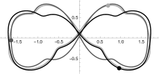
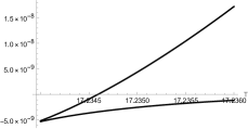
  (a)                                (b)                                      (c)

Figure 3: Orbits at $T=30$ for $y$-axis symmetric solution $q^{(b)^{2}}$ with $D_{2}\{{\cal M},\mu\}$ [21] and their action values, bifurcated at $T^{(b)^{2}}=17.240$ from $q^{(b)}$ with $C_{6h}\{{\cal CM},\mu\}$. (a) $q^{(b)^{2}}$ from the left side of bifurcation point, (b) from right side, and (c) action value $S(q^{(b)^{2}})-S(q^{(b)})$. Initial conditions: (a) $(x_{1},y_{1})=(0,0.10529629)$, $(x_{2},y_{2})=(1.5421890,0.45426224)$, $(\dot{x}_{1},\dot{y}_{1})=(0.30563750,-0.37778377)$ and $(\dot{x}_{2},\dot{y}_{2})=(-0.17440457,0.19744777)$. (b) $(x_{1},y_{1})=(0,0.0014326920)$, $(x_{2},y_{2})=(1.6469521,0.47710996)$, $(\dot{x}_{1},\dot{y}_{1})=(0.23166197,-0.38278558)$ and $(\dot{x}_{2},\dot{y}_{2})=(-0.12592133,0.18861645)$.

• 
  

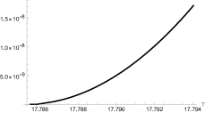
  (a)                                (b)                                      (c)

Figure 4: Orbits at $T=20$ for non-symmetric solution $q^{(b)^{2}}$ with $C_{2}\{\mu\}$ and their action values, bifurcated at $T^{(b)^{2}}=17.785$ from the $q^{(b)}$ with $C_{6h}\{{\cal CM},\mu\}$. (a) $q^{(b)^{2}}$ with higher action value, (b) with lower action value, and (c) their action values $S(q^{(b)^{2}})-S(q^{(b)})$. Initial conditions: (a) $(x_{1},y_{1})=(0,0.045)$, $(x_{2},y_{2})=(1.4396475,0.5347018)$, $(\dot{x}_{1},\dot{y}_{1})=(0.34271348,0.30563750)$ and $(\dot{x}_{2},\dot{y}_{2})=(-0.17598165,0.25858920)$. (b) $(x_{1},y_{1})=(0,0.045)$, $(x_{2},y_{2})=(1.4327086,0.40489872)$, $(\dot{x}_{1},\dot{y}_{1})=(0.35818585,-0.52798612)$ and $(\dot{x}_{2},\dot{y}_{2})=(-0.12592133,0.18861645)$.

In tables 9 and 10, bifurcation solution $q^{(b)^{2}}$ at $T^{(b)^{2}}=(T^{(b)})^{(b)}$ from $q^{(b)}$ at $T^{(b)}=18.615$, $17.132$ in table 8 are tabulated, respectively, in the same manner. Since $q^{(b)}$ is bifurcated by one side bifurcation from $q$, $q^{(b)}$ begins at the bifurcation point $T^{(b)}$.

Three planar solutions with symmetry $G(q^{(b)^{2}})=C_{6}\{\mu{\cal C}\}$, $D_{2}\{{\cal M},\mu\}$ and $C_{2}\{\mu\}$, in tables 9 and 10, are new type of solutions in our numerical calculations.

5.1.1 Non-symmetric choreography

The two-fold type bifurcation solution $q^{(b)^{2}}$ at $T^{(b)^{2}}=19.020$ in tables 9 with symmetry $G(q^{(b)^{2}})=C_{6}\{\mu{\cal C}\}$ is non-symmetric choreography. In figure 2, its non-symmetric orbit at $T=45$ with initial conditions is shown.

5.1.2 Three-fold type of $C_{3}$ representation

The three-fold type bifurcation solution $q^{(b)^{2}}$ at $T^{(b)^{2}}=17.240$ in table 10 with symmetry $G(q^{(b)^{2}})=D_{2}\{{\cal M},\mu\}$ has three separate $y$-axis symmetric orbits [21]. In figure 3, their orbits at $T=30$ with initial conditions and the action value $S(q^{(b)^{2}})-S(q^{(b)})$ around bifurcation point is shown. The solution to the left side of the bifurcation point soon turn back by fold bifurcation as other three-fold type [6].

This solution is the first numerical example with the three-fold type of $C_{3}$ representation where its $G(r;q^{(b)})$ does not depend on the direction of $r$, see $C_{3}\{C(3),+E\}$ in table 3 (a).

5.1.3 Six-fold type of $C_{6}$ representation

The six-fold type bifurcation solutions $q^{(b)^{2}}$ at $T^{(b)^{2}}=17.785$ in table 10 consist of two incongruent solutions with the same symmetry $G(q^{(b)^{2}})=C_{2}\{\mu\}$. In figure 4 (a) and (b), their orbits at $T=20$ with initial conditions are shown. The orbits of two solutions, (a) and (b), are very similar but not congruent and distinguishable. The both orbits are eight-shaped, however, have no spacial symmetry.

In figure 4 (c), their action values $S(q^{(b)^{2}})-S(q^{(b)})$ around bifurcation point are shown. However, since absolute difference of two values is too small compared with $|S(q^{(b)^{2}})-S(q^{(b)})|$ it is impossible to distinguish two curves in figure 4 (c).

This solution is the first numerical example with the six-fold type of $C_{6}$ representation where its $G(r;q^{(b)})$ does not depend on the direction of $r$ and two kinds of solutions have the same symmetry, see $C_{6}\{C(6),+E\}$ in table 3 (a).

5.2 Homogeneous potential system

Table 11: $q^{(b)}$ from $q$ with $D_{6h}\{{\cal CM},{\cal S},\mu\}$ for $u(r)=-1/r^{a}$.

• $a^{(b)}$		$\kappa$	$D$	$G(q^{(b)})$	side
  $-0.3817$		$\nearrow$	$D_{6}$	$D_{2}\{{\cal C}^{-n}{\cal SM},\mu\}$ $D_{2}\{{\cal C}^{1-n}{\cal S},\mu\}$
  $-0.2142$		$\nearrow$	$C_{2}$	$D_{6}\{\mu{\cal C},{\cal SM}\}$	R
  $0.9966$		$\nearrow$	$D_{3}$	$D_{2h}\{{\cal C}^{n-1}{\cal S},{\cal M},\mu\}$	B
  $1.3424$		$\nearrow$	$D_{6}$	$D_{2}\{{\cal C}^{-n}{\cal SM},\mu\}>D_{2}\{{\cal C}^{1-n}{\cal S},\mu\}$	R

In table 11, bifurcations calculated numerically for the system with the homogeneous potential

$$u(r)=-\frac{1}{r^{a}}$$ (101)

from the figure-eight choreography $q$ [6, 9], are shown in the same manner. The bifurcation parameter $\xi$ is the power $a$ and the bifurcation point $\xi^{(b)}$ is $a^{(b)}$ tabulated in the first column. Note that bifurcation at $a^{(b)}=-0.3817$ is identified by eigenvalue $\kappa$ and eigenfunction $\phi$ but the bifurcation solution is not calculated numerically, and its “side” and inequality between symmetries are empty.

Table 12: $q^{(b)^{2}}$ from $q^{(b)}$ with $D_{2h}\{{\cal C}^{n-1}{\cal S},{\cal M},\mu\}$, $n=1$, in table 11.

• $a^{(b)^{2}}$	branch	$\kappa$	$D$	$G(q^{(b)^{2}})$	side
  $0.9100$	$-$	$\swarrow$	$C_{2}$	$D_{2}\{{\cal S},\mu\}$	R
  $0.8156$	$0$	$(\uparrow$	$C_{1}$	$D_{2h}\{{\cal S},{\cal M},\mu\}$	B
  $0.8460$	$+$	$\nearrow$	$C_{2}$	$D_{2}\{\mu{\cal S},\mu{\cal M}\}$	L
  $0.9966$	$0$	$\searrow$	$C_{1}$	$D_{2h}\{{\cal S},{\cal M},\mu\}$	X
  $0.9966$	$0$	$\nearrow$	$C_{2}$	$D_{2}\{{\cal M},\mu\}$	X
  $1.0000$	$-$	Simó’s H		$D_{2h}\{{\cal S},{\cal M},\mu\}$
  $1.0272$	$0$	$\uparrow)$	$C_{1}$	$D_{2h}\{{\cal S},{\cal M},\mu\}$	B

• 

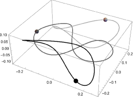
Figure 5: Orbit at $a=0.75$ for non-planar solution $q^{(b)^{2}}$ with $D_{2}\{\mu{\cal S},\mu{\cal M}\}$ bifurcated at $a^{(b)^{2}}=0.8460$ by two-fold type bifurcation from $q^{(b)}$ with $D_{2h}\{{\cal C}^{n-1}{\cal S},{\cal M},\mu\}$, $n=1$ in table 12 [15]. Initial conditions: $(x_{1},y_{1},z_{1})=(0.13030202,0.19616588,0.098259590)$, $(x_{2},y_{2},z_{2})=(-2x_{1},0,0)$, $(\dot{x}_{1},\dot{y}_{1},\dot{z}_{1})=(-v\cos\theta,-v\sin\theta,-0.013911923)$, $(\dot{x}_{2},\dot{y}_{2},\dot{z}_{2})=(0,-2\dot{y}_{1},-2\dot{z}_{1})$, $v=1.0045200$, $\theta=\arctan(y_{1},3x_{1})$ and $T=1$.

In table 12, bifurcation solution $q^{(b)^{2}}$ at $a^{(b)^{2}}=(a^{(b)})^{(b)}$ from $q^{(b)}$ at $a^{(b)}=0.9966$ shown in table 11 which becomes Simó’s H solution at $a=1$ [23] are tabulated. The row at $a^{(b)^{2}}=1.0000$ is not bifurcation but its indication. At $a^{(b)^{2}}=0.9966$, two eigenvalues for one-dimensional representation denoted by “X” in the “side” column cross. This is a point where the solutions $q^{(b)}$ bifurcate from $q$. We will comment on this in section 6.

5.2.1 Non-planar bifurcation solution

The two-fold type solution $q^{(b)^{2}}$ bifurcated at $a^{(b)^{2}}=0.8460$ with symmetry $G(q^{(b)^{2}})=D_{2}\{\mu{\cal S},\mu{\cal M}\}$ in table 12 is only non-planar solution among our numerical calculations [15], whereas there is non-planar solution by taking mass as bifurcation parameter [8]. Its orbit at $a=0.75$ is shown in figure 5 with initial conditions.

6 Summary and discussions

We could explain all bifurcations $q^{(b)^{k}}$ numerically observed from figure-eight choreography $q$ by the irreducible representation $D(q^{(b)^{k-1}})$ representing eigenspace of $H(q^{(b)^{k-1}})$. There are four types of bifurcation solutions. (i) the trivial type bifurcates two solutions in the both sides of bifurcation point in $\kappa$, sometimes in the fold-bifurcation in $\xi$. (ii) The two-fold type bifurcates two congruent solutions in one side. (iii) The three-fold type bifurcates two kinds of three congruent solutions in the both side. (iv) The six-fold type bifurcates two kinds of six congruent solutions in one side.

Note that in our preprint [9] though bifurcations are classified into six types I–VI, in this paper we combined three one-dimensional types II–IV in [9] into two-fold type, and the two two-dimensional types V and VI are extended to the three-fold and the six-fold types, respectively. Type I in [9] is the same as the trivial type in this paper.

Accordingly, we understand how to yield the bifurcation solution $q^{(b)}$ from the original solution $q$, however, we do not describe yet, inverse process, how to yield $q$ from $q^{(b)}$. From the numerical calculation, we observe that the inverse process will be represented by the eigenfunctions of $H(q^{(b)})$ with the same number and the same symmetry as the original process described by $H(q)$.

• 
  

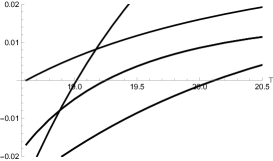
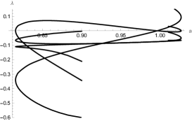
  (a)                                            (b)

Figure 6: Eigenvalues of $H(q^{(b)})$ (a) for $G(q^{(b)})=D_{6}\{\mu{\cal C},{\cal S}\}$ [21] and (b) for planar eigenfunctions for $G(q^{(b)})=D_{2h}\{{\cal S},{\cal M},\mu\}$ [22].

In figure 6 (a), eigenvalues of $H(q^{(b)})$ for $G(q^{(b)})=D_{6}\{\mu{\cal C},{\cal S}\}$ in table 2 are shown [21]. The eigenfunction of the curve going to zero toward $T=18.615$ has the same symmetry with $q^{(b)}$ and represents the inverse process. The original bifurcation is represented by one-dimensional eigenfunction with the same $D_{6}\{\mu{\cal C},{\cal S}\}$ symmetry.

In figure 6 (b), planar eigenvalues for $G(q^{(b)})=D_{2h}\{{\cal S},{\cal M},\mu\}$ in table 12 are shown [22]. The eigenfunctions of the non-degenerate two curves crossing at $a=0.9966$ have the same symmetries with the eigenfunctions representing original process, $D_{2h}\{{\cal C}^{n-1}{\cal S},{\cal M},\mu\}$, $n=1$ and $D_{2}\{{\cal M},\mu\}$ of doubly degenerate eigenvalue in table 1. As in the one-dimensional case in figure 6 (a), one of the eigenfunctions has the same symmetry with $q^{(b)}$.

Other than the processes from $q^{(b)}$ to $q$, we have never met the bifurcation represented by reducible representations. However, the current method should be extended to the reducible representations.

In numerical search, we found a non-planar bifurcation solution, which is unfortunately not choreographic, in the homogeneous interaction potential system. Though the LJ potential system possesses a lot of bifurcations, we could not find any non-planar solution. We do not know the reason why the remarkable, up to now theoretically possible, “non-planar figure-eight choreographic” bifurcation solution is not found.

Our method of analysis will be applicable to the bifurcation of the periodic solution for general few body system if it has symmetries.

References

References

- [1] Moore C 1993 Phys. Rev. Lett. 70 3675–3679
- [2] Chenciner A and Montgomery R 2000 Annals of Mathematics 152(3) 881–901
- [3] Sbano L 2004 Symmetry and Perturbation Theory 291–299
- [4] Sbano L and Southall J 2010 Dynamical Systems 25(1) 53–73
- [5] Fukuda H, Fujiwara T and Ozaki H 2017 J. Phys. A: Math. Theor. 50, 105202
- [6] Fukuda H, Fujiwara T and Ozaki H 2019 J. Phys. A: Math. Theor. 52, 185201
- [7] Galán J, Muñoz-Almaraz F J, Freire E, Doedel E and Vanderbauwhede A 2002 Phys. Rev. Lett. 88 241101-1–4
- [8] Doedel E J, Paffenroth R C, Keller H B, Dichmann D J and Galán-Vioque J 2003 International Journal of Bifurcation and Chaos 13 No. 6 1353–1381
- [9] Fujiwara T, Fukuda H and Ozaki H 2020 arXiv:2002.03496v3 [math-ph]
- [10] Chenciner A, Féjoz J and Montgomery R 2005 Nonlinearity 18 1407–1424
- [11] Golubitsky M and Schaeffer D G 1984 Singularities and Groups in Bifurcation Theory I (Springer New York, NY)
- [12] Golubitsky M, Stewart I and Schaeffer D G 1988 Singularities and Groups in Bifurcation Theory II (Springer New York, NY)
- [13] Ikeda K and Murota K 2019 Imperfect Bifurcation in Structures and Materials (Springer Cham)
- [14] Sattinger D H 1979 Group Theoretic Methods in Bifurcation Theory (Springer Berlin, Heidelberg)
- [15] Fukuda H, Fujiwara T and Ozaki H 2020 The Japan Society for Industrial and Applied Mathematics, Annual Meeting, Proceedings 252–253
- [16] Wintner A 1941 The Analytical Foundations of Celestial Mechanics (Princeton University Press)
- [17] Siegel C L and Moser J K 1971 Lectures on Celestial Mechanics (Springer Berlin, Heidelberg)
- [18] Harris D and Bertolucci M 1989 Symmetry and Spectroscopy (New York: Dover Publications)
- [19] Wolfram Research Inc. 2024 Mathematica, Version 14.0, Champaign, IL
- [20] Fukuda H, Fujiwara T and Ozaki H 2018 J. Phys. A: Math. Theor. 51, 145201
- [21] Fukuda H, Fujiwara T and Ozaki H 2023 10th International Congress on Industrial and Applied Mathematics, ICIAM 2023 Tokyo
- [22] Fukuda H, Fujiwara T and Ozaki H 2019 Symposium on Celestial Mechanics in Sagamihara
- [23] Simó C 2002 Contemporary mathematics, 292 209–228