Loss Gradient Gaussian Width based
Generalization and Optimization Guarantees

Arindam Banerjee
Department of Computer Science
University of Illinois at Urbana-Champaign
arindamb@illinois.edu
   Qiaobo Li
Department of Computer Science
University of Illinois at Urbana-Champaign
qiaobol2@illinois.edu
   Yingxue Zhou
Department of Computer Science
University of Minnesota, Twin Cities
zhou0877@umn.edu
Abstract

Generalization and optimization guarantees on the population loss in machine learning often rely on uniform convergence based analysis, typically based on the Rademacher complexity of the predictors. The rich representation power of modern models has led to concerns about this approach. In this paper, we present generalization and optimization guarantees in terms of the complexity of the gradients, as measured by the Loss Gradient Gaussian Width (LGGW). First, we introduce generalization guarantees directly in terms of the LGGW under a flexible gradient domination condition, which we demonstrate to hold empirically for deep models. Second, we show that sample reuse in finite sum (stochastic) optimization does not make the empirical gradient deviate from the population gradient as long as the LGGW is small. Third, focusing on deep networks, we present results showing how to bound their LGGW under mild assumptions. In particular, we show that their LGGW can be bounded (a) by the $L_{2}$-norm of the loss Hessian eigenvalues, which has been empirically shown to be $\tilde{O}(1)$ for commonly used deep models; and (b) in terms of the Gaussian width of the featurizer, i.e., the output of the last-but-one layer. To our knowledge, our generalization and optimization guarantees in terms of LGGW are the first results of its kind, avoid the pitfalls of predictor Rademacher complexity based analysis, and hold considerable promise towards quantitatively tight bounds for deep models.

1 Introduction

Machine learning theory typically characterizes generalization behavior and related aspects in terms of uniform convergence guarantees, often in terms of Rademacher complexities of predictor function classes [44, 9, 73, 60]. However, given the rich representation power of modern deep models, it has been difficult to develop sharp uniform bounds, and concerns have been raised whether non-vacuous bounds following the uniform convergence route may be possible [61, 62, 43, 42, 11, 31]. On the other hand, the empirical successes of deep learning has highlighted the importance of gradients, which play a critical role in learning over-parameterized models with deep representations [14, 32, 45]. The motivation behind this paper is to investigate generalization and optimization guarantees based on uniform convergence analysis of gradients, rather than the predictors.

Empirical work in recent years has demonstrated that gradients of overparameterized deep learning models are typically “simple,” e.g., only a small fraction of entries have large values [64, 65, 47, 86, 88], gradients typically lie in a low-dimensional space [33, 29, 71, 39], using top-$k$ components with suitable bias corrections work well in practice [71, 39], etc. In this paper, we view such simplicity in terms of the loss gradient Gaussian width (LGGW) [80, 83]. Based on the empirical evidence, we posit that loss gradients of modern machine learning models have small Gaussian widths. Our main technical results in the paper present generalization and optimization guarantees for learning in terms of the LGGW. While our main technical results hold irrespective of whether the LGGW is small or not, similar to their classical Rademacher complexity counterparts, the results imply sharper bounds if the LGGW is small. Further, while deep learning gradients form the motivation behind the work, some of the technical results we present are not restricted to deep learning and hold for general models under simple regularity conditions.

In Section 2, we present generalization bounds in terms of the LGGW. Our analysis needs a mechanism to transition from losses to gradients of losses, and we assume the population loss function satisfies a flexible gradient domination (GD) condition [27], which includes the PL (Polyak-Łojasiewicz) condition [66] used in modern deep learning [50, 53, 49] as a simple special case. We empirically demonstrate that GD holds for commonly used deep models. Then, based on recent advances in uniform convergence of gradients and, more generally, vector-valued functions [56, 57, 27], one can readily get generalization bounds based on the vector Rademacher complexity of gradients. Our main new result on generalization is to show that such vector Rademacher complexity can be bounded by the LGGW, which makes the bound explicitly depend on the geometry of gradients. The result may seem surprising at first as the expectation of randomness in vector Rademacher complexity is over $n$ Rademacher variables $\{\varepsilon_{i},i\in[n]\}$ corresponding to the samples whereas the expectation of randomness in Gaussian width is over $p$ Gaussian variables $\mathbf{g}\sim{\cal N}(0,\mathbb{I}_{p\times p})$ corresponding to the $p$ parameters in the model. Our proof is based on generic chaining (GC) [80], where we first bound the vector Rademacher complexity using a hierarchical covering argument, and then bound the hierarchical covering in terms of the Gaussian width using the majorizing measure theorem [80]. To our knowledge, this is the first generalization bound in terms of Gaussian width of loss gradients, and the results imply that models with small LGGW will generalize well.

In Section 3, we present optimization guarantees based on the LGGW. One of the arguably biggest disconnects between the theory and practice of (mini-batch) stochastic gradient descent (SGD) is that the theory assumes a mini-batch of fresh samples in each step whereas in practice one reuses samples. If one just focuses on the finite sum empirical risk minimization (ERM), sample reuse is not an issue. However, the goal of such optimization is to reduce the population loss, and sample reuse derails the standard analysis. We show that even with sample reuse, the discrepancy between the (mini-batch) sample average and the population gradient can be bounded by the LGGW along with only a logarithmic dependence on how many times the sample has been reused. Thus, if the LGGW is small, the sample average gradients stay close to the population gradients, even under sample reuse. We establish such results for both full-batch and mini-batch, and use these results to establish population convergence results for mini-batch gradient descent with sample reuse. Since our bounds are uniform, there is no dependence on the mechanism by which the mini-batches are selected, e.g., random draw with replacement [34, 67], permute/shuffle and draw without replacement [54, 72], etc.

In Section 4, we present the first results on bounding LGGW of deep learning gradients. Recent empirical work has demonstrated sharply decaying eigenvalues of the loss Hessian [92, 87, 89]. Based on such observations, our first result is to show that the LGGW can be bounded by an upper bound on the $L_{2}$-norm of the loss Hessian eigenvalues, which has been empirically shown to be $\tilde{O}(1)$ for commonly used deep models  [92, 87]. Further, we consider formal models for feed-forward and residual networks widely studied in the deep learning theory literature [1, 21, 7, 51, 8] and show that their LGGW can be bounded by the Gaussian width of the featurizer, i.e., the output of the last-but-one layer. The results emphasize the benefits of Hessian eigendecay and the simplicity as well as stability of featurizers for deep learning.

A brief word on notation: $c_{1},c_{2},c_{3}$, etc., denote constants, and they may mean different constants at different places. Such repeat use of constants is common in the GC literature [80]. We use $\tilde{O}$ to hide poly-log terms. The exact dependencies are in the proofs in the Appendix.

2 Gaussian Width based Generalization Bounds

In this section, we formalize the notion of Loss Gradient Gaussian Width (LGGW) [83, 80], and as the main result, establish generalization bounds in terms of LGGW. For parameters $\theta\in\Theta\subset\mathbb{R}^{p}$ and data points $z\in{\cal Z}$ where $z=(\mathbf{x},y),\mathbf{x}\in\mathbb{R}^{d},y\in\mathbb{R}$, for any suitable loss $\ell(\theta;z):\Theta\times{\cal Z}\mapsto\mathbb{R}_{+}$, the gradients of interest are $\xi(\theta;z)=\nabla_{\theta}\ell(\theta;z)\in\mathbb{R}^{p}$. Given a dataset of $n$ samples, we start by defining the sets of all empirical average gradients and $n$-tuple of individual gradients:

Definition 1 (Gradient Sets).

Given $n$ samples $z^{(n)}=\{z_{1},\ldots,z_{n}\}\in{\cal Z}^{(n)}$, for a suitable choice of parameter set $\Theta$ and loss $\ell:\Theta\times{\cal Z}\mapsto\mathbb{R}_{+}$, let the set of all possible empirical average and $n$-tuple of individual loss gradients be respectively denoted as:

$\displaystyle\hat{\Xi}_{n}(\Theta)$ $\displaystyle:=\left\{\hat{\xi}_{n}\in\mathbb{R}^{p}\mid\exists\theta\in\Theta~{}~{}~{}\text{s.t.}~{}~{}\hat{\xi}_{n}=\frac{1}{n}\sum_{i=1}^{n}\nabla\ell(\theta;z_{i})\right\}~{},$ (1)
$\displaystyle\hat{\Xi}^{(n)}(\Theta)$ $\displaystyle:=\left\{\hat{\xi}^{(n)}=\{\xi_{i},i\in[n]\}\mid\exists\theta\in\Theta~{}\text{s.t.}~{}\xi_{i}=\nabla\ell(\theta;z_{i})\right\}~{}.$ (2)

For convenience, we will denote the empirical average gradient in (1) as $\hat{\Xi}_{n}$, and the set of $n$-tuples of gradients in (2) as $\hat{\Xi}^{(n)}$. Note that the sets $\hat{\Xi}_{n}$ and $\hat{\Xi}^{(n)}$ are conditioned on $z^{(n)}$, and the results we will present will hold for any $z^{(n)}\subset{\cal Z}^{n}$, i.e., any $n$ samples under suitable regularity conditions (see Section 4.2.1). We use $\hat{\xi}_{n}(\theta)$ and $\hat{\xi}_{n}$ interchangeably to denote the n sample average gradient. Next, we define the Loss Gradient Gaussian Width:

Definition 2 (Loss Gradient Gaussian Width).

Given the empirical average gradient set $\hat{\Xi}_{n}$ as in Definition 1, the loss gradient Gaussian width (LGGW) is defined as:

$\displaystyle w(\hat{\Xi}_{n}):=\mathbb{E}_{\mathbf{g}\sim{\cal N}(0,\mathbb{I}_{p\times p})}\left[\sup_{\hat{\xi}_{n}\in\hat{\Xi}_{n}}~{}\langle\hat{\xi}_{n},\mathbf{g}\rangle\right]~{}.$ (3)

2.1 Bounds based on Vector Rademacher Complexity

Our approach to generalization bounds is based on vector Rademacher complexities. Unlike the traditional approach which focus on bounds based on Rademacher complexities of the set of predictors $f(\theta;x)$ [44, 9, 73, 60], we will develop generalization bounds based on vector Rademacher complexities [56, 57, 27] of the set of loss gradients $\xi(\theta,z)=\nabla\ell(\theta;z)$. In particular, following [27], we consider Normed Empirical Rademacher Complexity (NERC), which is the extension of standard Rademacher complexity to sets of vectors or vector-valued functions.

Definition 3.

In the setting of Definition 1, for the set $\hat{\Xi}^{(n)}$ of $n$-tuples of individual gradients, the Normed Empirical Rademacher Complexity (NERC) is defined as

$\displaystyle\hat{R}_{n}(\hat{\Xi}^{(n)})$ $\displaystyle:=\frac{1}{n}\mathbb{E}_{\varepsilon^{(n)}}\left[\sup_{\hat{\xi}^{(n)}\in\hat{\Xi}^{(n)}}\left\|\sum_{i=1}^{n}\varepsilon_{i}\xi_{i}\right\|~{}\right]~{},$ (4)

where $\varepsilon^{(n)}$ are a set of $n$ i.i.d. Rademacher random variables, i.e., $P(\varepsilon_{i}=+1)=P(\varepsilon_{i}=-1)=\frac{1}{2}$, and $\hat{\Xi}^{(n)}$ is the set of $n$-tuples of gradients as in (2).

For (4), we present results for the $L_{2}$ norm $\|\cdot\|_{2}$, but the analyses tools and results have counterparts for general norms [46] and such results will be in terms of $\gamma$-functions in generic chaining [80].

Given a loss function $\ell$ and a distribution ${\cal D}$ over examples $z\in{\cal Z}$, we consider the minimization of the population risk function, that is,

$$\min_{\theta}{\cal L}_{{\cal D}}(\theta):=\mathbb{E}_{z\sim{\cal D}}\left[\ell(\theta;z)\right].$$ (5)

The learner does not observe the distribution ${\cal D}$ and typically minimize the empirical risk

$$\hat{\cal L}_{n}(\theta):=\frac{1}{n}\sum_{i=1}^{n}\ell(\theta;z_{i}),$$ (6)

where $z^{(n)}\sim{\cal D}^{n}$ are i.i.d. draws. While the loss functions are usually non-convex in modern machine learning, including deep learning, they usually satisfy a form of the gradient domination (GD) condition [27], which includes the popular Polyak-Łojasiewicz (PL) condition as a simple special case [66, 50, 53, 49]. Further, we assume the gradients to be bounded.

Assumption 1 (Population Risk: Gradient Domination).

The population risk ${\cal L}_{\cal D}$ satisfies the $(\alpha,\bar{c}_{\alpha})$-GD condition with respect to a norm $\|\cdot\|$, if there are constants $\bar{c}_{\alpha}>0$, $\alpha\in[1,2]$, such that $\forall\theta\in\Theta$ and $\theta^{\star}\in\operatorname{argmin}_{\theta\in\Theta}{\cal L}_{\mathcal{D}}(w)$, we have

$\displaystyle{\cal L}_{\mathcal{D}}(\theta)-{\cal L}_{\mathcal{D}}\left(\theta^{\star}\right)\leq\bar{c}_{\alpha}\left\|\nabla{\cal L}_{\mathcal{D}}(\theta)\right\|^{\alpha}~{}.$ (7)
Assumption 2 (Bounded Gradients).

The sample gradients $\xi(\theta;z)=\nabla\ell(\theta;z)$ are bounded, i.e., $\|\xi(\theta;z)\|_{2}=O(1),\theta\in\Theta,z\in{\cal Z}$.

Remark 2.1.

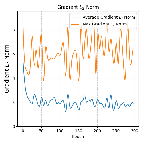
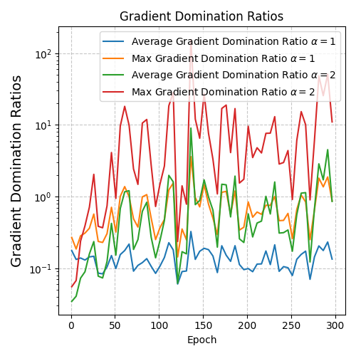
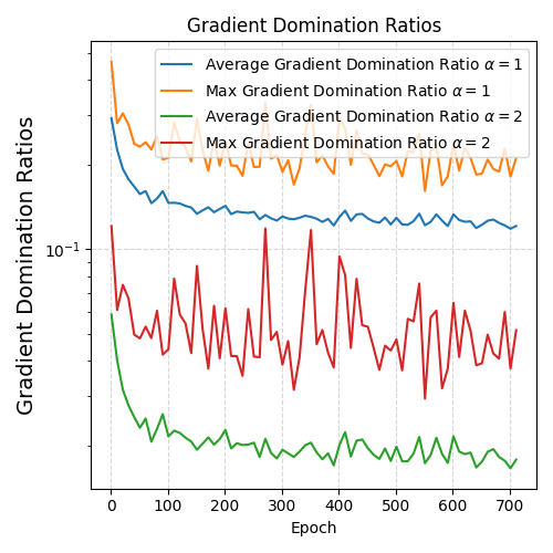
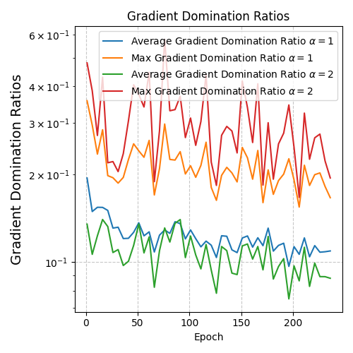
It is practically important is to understand whether the $(\alpha,\bar{c}_{\alpha})$-GD condition in Assumption 1 holds for widely used models, e.g., modern deep learning models. In Figure 1, we plot the gradient domination ratio $\frac{{\cal L}_{\mathcal{D}}(\theta)}{\left\|\nabla{\cal L}_{\mathcal{D}}(\theta)\right\|^{\alpha}}$ for $\alpha=1,2$ for three standard deep learning models. The plots demonstrate that the condition indeed clearly holds for $\alpha=1$ with a small constant $\bar{c}_{1}<5$ for all models, and for $\alpha=2$, i.e., the PL condition [66, 50, 53, 49], with $\bar{c}_{2}<1$ for some models, but needs large constants $\bar{c}_{2}>100$ for for ResNet18 on CIFAR-10. We establish results for any $\alpha\in[1,2]$, which along with the empirical evidence for $\alpha=1$ makes the Assumption 1 valid. ∎

Refer to caption
(a) ResNet18 on CIFAR-10
Refer to caption
(b) FFN on CIFAR-10
Refer to caption
(c) CNN on Fashion-MNIST
Figure 1: Gradient Domination Ratio for $\alpha=1,2$ for (a) ResNet18 on CIFAR-10, (b) FFN on CIAFR-10 and (c) CNN on Fashion-MNIST. Each experiment is repeated 5 times and we report the average and the maximum ratio. The results demonstrate that the gradient domination condition indeed clearly holds for $\alpha=1$ with a small constant $\bar{c}_{1}<5$ for all models, and for $\alpha=2$, with $\bar{c}_{2}<1$ for some models, but needs large constants $\bar{c}_{2}>100$ for for ResNet18.

We start with a generalization bound from [27] for losses satisfying gradient domination.

Proposition 1.

Under Assumptions 1 and 2, with $\theta^{\star}\in\operatorname{argmin}_{\theta\in\Theta}{\cal L}_{\mathcal{D}}(\theta)$ denoting any population loss minimizer and $\hat{R}_{n}(\hat{\Xi}^{(n)})$ as in Definition 3, for any $\delta>0$, with probability at least $1-\delta$ over the draw of the samples $z^{(n)}\sim{\cal D}^{n}$, for any $\hat{\theta}\in\Theta$ we have

$${\cal L}_{{\cal D}}(\hat{\theta})-{\cal L}_{{\cal D}}(\theta^{*})\leq 2\bar{c}_{\alpha}\bigg{(}\|\nabla\hat{{\cal L}}_{n}(\hat{\theta})\|_{2}^{\alpha}+2\left(4\hat{R}_{n}(\hat{\Xi}^{(n)})+c_{3}\frac{\log\frac{1}{\delta}}{n}\right)^{\alpha}\bigg{)}+c_{4}\left(\frac{\log\frac{1}{\delta}}{n}\right)^{\frac{\alpha}{2}}$$ (8)

For such a bound to be useful, the NERC $\hat{R}_{n}(\Xi^{(n)})$ needs to be small, e.g., $\hat{R}_{n}(\hat{\Xi}^{(n)})=O(\frac{1}{\sqrt{n}})$. [27] analyzed the NERC for loss functions of the form $\ell(\theta,(x,y))=h(\psi_{\theta}(x))$, where $\psi_{\theta}(x)=\langle\theta,x\rangle$ and $h$ is Lipschitz. For this case, it suffices to bound the NERC of the gradient of linear predictor $\psi_{\theta}(x)=\theta^{T}x$. Since $\nabla\psi_{\theta}(x)=x$ is independent of $\theta$, as long as each $\|x_{i}\|$ is bounded (Assumption 2), we have $\frac{1}{n}\mathbb{E}_{\varepsilon^{(n)}}\left[\sup_{\theta\in\Theta}\left\|\sum_{i=1}^{n}\varepsilon_{i}\nabla\phi(\theta,x_{i})\right\|\right]=\frac{1}{n}\mathbb{E}_{\varepsilon^{(n)}}\left[\left\|\sum_{i=1}^{n}\varepsilon_{i}x_{i}\right\|\right]=\frac{c}{\sqrt{n}}$, by Khintchine’s inequality [46, 82] for $L_{2}$ norm and under suitable assumptions on certain other norms [43, 42, 27]. The key simplification here is that the $\sup_{\theta\in\Theta}$ drops out since the gradient does not depend on $\theta$. However, the simplification is only possible for linear predictors. To go beyond, our analysis considers the general case where the $\sup_{\theta}$ does not drop out, and has to handled explicitly.

2.2 Main Result: Gaussian Width Bound

For our main result, we consider whether the NERC $\hat{R}_{n}(\hat{\Xi}^{(n)})$ can somehow be related to the Gaussian width $w(\hat{\Xi}_{n})$ as in (1), which arguably captures the geometry of the gradients more directly.

Theorem 1.

Based on Definitions 1, 2, and 3, with $\varepsilon^{(n)}$ denoting $n$ i.i.d. Rademacher variables, conditioned on any $z^{(n)}\in{\cal Z}^{(n)}$, for any $u>0$, with probability at least $(1-c_{0}\exp(-u^{2}/2))$ over the randomness of $\varepsilon^{(n)}$, we have

$\displaystyle\sup_{\hat{\xi}^{(n)}\in\hat{\Xi}^{(n)}}\frac{1}{\sqrt{n}}\left\|\sum_{i=1}^{n}\varepsilon_{i}\xi_{i}\right\|_{2}\leq c_{5}(1+u)w(\hat{\Xi}_{n})~{}.\vspace*{-2mm}$ (9)

As a result, the normed empirical Rademacher complexity (NERC) satisfies

$$\hat{R}_{n}(\hat{\Xi}^{(n)})=\frac{1}{n}\mathbb{E}_{\varepsilon^{(n)}}\left[\sup_{\hat{\xi}^{(n)}\in\hat{\Xi}^{(n)}}\left\|\sum_{i=1}^{n}\varepsilon_{i}\xi_{i}\right\|_{2}\right]\leq\frac{c_{6}w(\hat{\Xi}_{n})}{\sqrt{n}}~{}.$$ (10)

One can plug-in the Theorem 1 to Proposition 1 to get the desired generalization bound. For example, with Assumption 1 holding for $\alpha=1$ (Figure 1), with probability $(1-\delta)$, for any $\hat{\theta}\in\Theta$ we have

$${\cal L}_{{\cal D}}(\hat{\theta})-{\cal L}_{{\cal D}}(\theta^{*})\leq 2\bar{c}_{1}\left(\|\nabla\hat{{\cal L}}_{n}(\hat{\theta})\|_{2}+2\left(\frac{4c_{6}w(\hat{\Xi}_{n})}{\sqrt{n}}+c_{3}\frac{\log\frac{1}{\delta}}{n}\right)\right)+c_{4}\sqrt{\frac{\log\frac{1}{\delta}}{n}}~{}.$$ (11)
Remark 2.2.

A technically curious aspect of the result in (10) is that the randomness in $\hat{R}_{n}(\hat{\Xi}^{(n)})$ is from $n$ Rademacher variables over samples whereas that in $w(\hat{\Xi}_{n})$ is from $p$ normal variables over gradient components. The shift from samples to gradient components makes the bound geometric. ∎

Remark 2.3.

It is important to understand that the bound in (11) does not depend on the algorithm used to reach $\hat{\theta}\in\Theta$. Thus, one can use variants of stochastic gradient descent, adaptive optimization, or sharpness aware minimization [90, 69, 25] to reach $\hat{\theta}$, and the bound would still hold. ∎

Remark 2.4.

For the result to be meaningful, $\Theta$ needs to be suitably chosen, without using the training set. For example, for deep learning models, $\Theta$ can constitute parameters encountered in the last 10% of epochs during training. There is empirical evidence showing loss gradients close to convergence have small norms and the loss Hessians, which capture the change in gradients, have sharply decaying eigenvalues. We review and build on such results in Section 4. ∎

2.3 Proof sketch of Main Result

Our analysis is based on generic chaining (GC) and needs the following key definition due to [80].

Definition 4.

For a metric space $(T,d)$, an admissible sequence of $T$ is a collection of subsets of $T$, $\Gamma=\{T_{r}:r\geq 0\}$, with $|T_{0}|=1$ and $|T_{r}|\leq 2^{2^{r}}$ for all $r\geq 1$. For $\beta\geq 1$, the $\gamma_{\beta}$ functional is defined by

$$\gamma_{\beta}(T,d):=\inf_{\Gamma}\sup_{t\in T}\sum_{r=0}^{\infty}2^{r/\beta}d(t,T_{r})~{},$$ (12)

where the infimum is over all admissible sequences $\Gamma$ of $T$.

Remark 2.5.

There has been substantial developments on GC over the past two decades [80, 81]. GC lets one develop sharp upper bounds to suprema of stochastic processes indexed in a set with a metric structure in terms of $\gamma_{\beta}$ functions. Typically, the bounds are in terms of $\gamma_{2}$ functions for sub-Gaussian processes and a mix of $\gamma_{1}$ and $\gamma_{2}$ functions for sub-exponential processes. ∎

To get to and understand the proof of Theorem 1, we first recap the standard GC argument. For any suitable stochastic process under consideration, say $\{X_{\xi}\}$, the key step is to find a suitable pseudo-metric $d(\xi_{1},\xi_{2})$ that satisfies increment condition (IC) [80]: for any $u>0$

$$\mathbb{P}(|X_{\xi_{1}}-X_{\xi_{2}}|\geq ud(\xi_{1},\xi_{2}))\leq 2\exp(-u^{2}/2)~{}.$$ (13)

Then, under some simple assumptions, e.g., $X_{\xi}=0$ for some $\xi\in\Xi$, GC shows that $\mathbb{E}[\sup_{\xi\in\Xi}X_{\xi}]\leq c\gamma_{2}(\Xi,d)$, for some constant $c$, and there is a corresponding high probability version of the result [80]. The analysis is typically done using the canonical distance

$\displaystyle d(\xi_{1},\xi_{2}):=(\mathbb{E}[(X_{\xi_{1}}-X_{\xi_{2}})^{2}])^{1/2}~{},$ (14)

though one can use other (not canonical) distance $\bar{d}(\xi_{1},\xi_{2})$ which satisfies the increment condition (13).

At a high level, our proof has three parts:

  • Since the NERC $\hat{R}_{n}(\hat{\Xi}^{(n)})$ is defined in terms of the set of $n$-tuples $\hat{\Xi}^{(n)}$, we start with a suitable (non canonical) distance $\bar{d}^{(n)}(\hat{\xi}^{(n)}_{1},\hat{\xi}^{(n)}_{2})$ over $n$-tuples in $\hat{\Xi}^{(n)}$ and establish a version of Theorem 1 in terms of $\gamma_{2}(\hat{\Xi}^{(n)},\bar{d}^{(n)})$, showing $\hat{R}_{n}(\hat{\Xi}^{(n)})\leq c_{2}\frac{\gamma_{2}(\hat{\Xi}^{(n)},\bar{d}^{(n)})}{\sqrt{n}}$.

  • For the set $\hat{\Xi}_{n}$ of average gradients $\hat{\xi}_{n}$, we construct a Gaussian process $X_{\hat{\xi}_{n}}=\langle\hat{\xi}_{n},\mathbf{g}\rangle$ where $\mathbf{g}\sim{\cal N}(0,\mathbb{I}_{p\times p})$. We note a simple one-to-one correspondence between the set of average gradients $\hat{\Xi}_{n}$ and the set of $n$-tuples $\hat{\Xi}^{(n)}$ since $\hat{\xi}_{n}=\frac{1}{n}\sum_{i=1}^{n}\xi_{i}$. Further, we show that the canonical distance $d(X_{\hat{\xi}_{1,n}},X_{\hat{\xi}_{2,n}})$ as in (14) from the Gaussian process on $\hat{\Xi}_{n}$ satisfies $d(X_{\hat{\xi}_{1,n}},X_{\hat{\xi}_{2,n}})=\bar{d}^{(n)}(\hat{\xi}^{(n)}_{1},\hat{\xi}^{(n)}_{2})$, the non-canonical distance on $\hat{\Xi}^{(n)}$. Based on the set correspondence and exact same distance measure, we have $\gamma_{2}(\hat{\Xi}_{n},d)=\gamma_{2}(\hat{\Xi}^{(n)},\bar{d}^{(n)})$, so that $\hat{R}_{n}(\hat{\Xi}^{(n)})\leq c_{2}\frac{\gamma_{2}(\hat{\Xi}_{n},d)}{\sqrt{n}}$.

  • The final step of the analysis is to show that $\gamma_{2}(\hat{\Xi}_{n},d)\leq c_{4}w(\hat{\Xi}_{n})$. The result follows directly from the Majorizing Measure Theorem [80] since we are working with a Gaussian process indexed on $\hat{\Xi}_{n}$ and using the canonical distance $d$.

We provide additional details and associated Lemma for the first part of the analysis. Consider the stochastic process $X_{\hat{\xi}^{(n)}}:=\frac{1}{\sqrt{n}}\left\|\sum_{i=1}^{n}\varepsilon_{i}\xi_{i}\right\|_{2}$, by triangle inequality, we have

$\displaystyle\left|X_{\hat{\xi}^{(n)}_{1}}-X_{\hat{\xi}^{(n)}_{2}}\right|\leq\frac{1}{\sqrt{n}}\left\|\sum_{i=1}^{n}\varepsilon_{i}(\xi_{i,1}-\xi_{i,2})\right\|_{2}~{}.$ (15)

Thus, for a suitable (non canonical) metric $\bar{d}^{(n)}(\hat{\xi}^{(n)}_{1},\hat{\xi}^{(n)}_{2})$, it suffices to show an increment condition (IC) of the form: for any $u>0$, with probability at least $1-2\exp(-u^{2}/2)$ over the randomness of $\varepsilon^{(n)}$, we have

$$\frac{1}{\sqrt{n}}\left\|\sum_{i=1}^{n}\varepsilon_{i}(\xi_{i,1}-\xi_{i,2})\right\|_{2}\leq u\bar{d}^{(n)}(\hat{\xi}^{(n)}_{1},\hat{\xi}^{(n)}_{2})~{}.$$ (16)

The in-expectation version of such a result is usually easy to establish using Jensen’s inequality, e.g., see (26.16) in [73]. The high probability version can be more tricky. We focus on a variant of the increment condition which allows for a constant shift, i.e., right hand side of the form $(\mu+u)\bar{d}^{(n)}(\hat{\xi}^{(n)}_{1},\hat{\xi}^{(n)}_{2})$ where $\mu=O(1)$. First, we consider the non-cannnical distance

$\displaystyle\bar{d}^{(n)}(\hat{\xi}^{(n)}_{1},\hat{\xi}^{(n)}_{2}):=\left(\frac{1}{n}\sum_{i=1}^{n}\|\xi_{i,1}-\xi_{i,2}\|_{2}^{2}\right)^{1/2}$ (17)

which is greater or equal to the canonical distance as in (14), due to Jensen’s inequality in (15). With our choice of distance $\bar{d}^{(n)}$, note that $\mathbf{v}_{i}=\frac{\xi_{i,1}-\xi_{i,2}}{\bar{d}^{(n)}(\hat{\xi}^{(n)}_{1},\hat{\xi}^{(n)}_{2})}$ satisfies $\sum_{i=1}^{n}\|\mathbf{v}_{i}\|^{2}_{2}=n$. Then, the following result is effectively a shifted increment condition (SIC), a shifted variant of (16) with a constant shift of $\mu\leq 1$:

Lemma 1.

Let $\mathbf{v}_{i}\in\mathbb{R}^{p},i=1,\ldots,n$ be a set of vectors such that $\sum_{i=1}^{n}\|\mathbf{v}_{i}\|^{2}_{2}\leq n$. Let $\varepsilon_{i}$ be a set of i.i.d. Rademacher random variables. Then, for any $u>0$,

$$\mathbb{P}_{\varepsilon^{(n)}}\left(\left|\left\|\frac{1}{\sqrt{n}}\sum_{i=1}^{n}\varepsilon_{i}\mathbf{v}_{i}\right\|_{2}-\mu\right|\geq u\right)\leq 2\exp\left(-\frac{u^{2}}{2}\right),$$ (18)

where $\mu\leq 1$ is a positive constant.

Next, we show that such constant shifts can be gracefully handled by GC:

Lemma 2.

Consider a stochastic process $\{X_{\hat{\xi}^{(n)}}\},\hat{\xi}^{(n)}\in\hat{\Xi}^{(n)}$ which satisfies: for any $u>0$, with probability at least $1-c_{1}\exp(-u^{2}/2)$, we have

$$\left|X_{\hat{\xi}^{(n)}_{1}}-X_{\hat{\xi}^{(n)}_{2}}\right|\leq c_{0}(\mu+u)\bar{d}^{(n)}\left(\hat{\xi}^{(n)}_{1},\hat{\xi}^{(n)}_{2}\right)~{}.$$ (19)

Further, assume that $X_{\hat{\xi}^{(n)}_{0}}=0$ for some $\hat{\xi}^{(n)}_{0}\in\hat{\Xi}^{(n)}$. Then, for any $u>0$, with probability at least $1-c_{3}\exp(-u^{2}/2)$, we have

$$\sup_{\hat{\xi}^{(n)}\in\hat{\Xi}^{(n)}}\left|X_{\hat{\xi}^{(n)}}\right|\leq c_{2}(\mu+u)\gamma_{2}\left(\hat{\Xi}^{(n)},\bar{d}^{(n)}\right)~{}.$$ (20)
Remark 2.6.

The $X_{\hat{\xi}^{(n)}_{0}}=0$ is easy to satisfy for gradients as long as the gradients are all zero for some $\theta_{0}$, e.g., minima of the loss, interpolation condition, etc. That condition is not necessary, and a more general result can be established, e.g., see [80][Theorem 2.4.12]. ∎

The SIC in Lemma 1 and the shifted variant of GC in Lemma 20 can now be used to establish the first part of the proof of Theorem 1. The technicalities for the other parts are more straightforward and are directly handled in the proof of Theorem 1.

3 SGD with Sample Reuse

Stochastic gradient descent (SGD) updates parameters following $\theta_{t+1}=\theta_{t}-\eta_{t}\nabla\ell(\theta_{t},z_{t}^{(b)})$, where $z_{t}^{(b)}$ are a mini-batch of $b$ fresh samples drawn from the underlying distribution ${\cal D}$. The mini-batch stochastic gradient is assumed to be unbiased. In practice, however, one reuses samples, by repeatedly drawing $z_{t}^{(b)}$ from a fixed set of $n$-samples $z^{(n)}=\{z_{1},\ldots,z_{n}\}$ drawn i.i.d. from ${\cal D}$ at the beginning. Such sample reuse violates the fresh sample assumption, and in turn cannot assume the mini-batch SGs to be unbiased [18, 77]. The theory and practice of SGD and variants have diverged: the theory continues to assume fresh samples [90, 28] whereas in practice one does multiple passes (epochs) over the fixed $z^{(n)}$ [34, 72]. Such sample reuse can be viewed as empirical risk minimization (ERM) [75, 73, 28, 63] where the analysis is focused only on the finite-sum objective, and one needs to use uniform convergence (UC) to get population results [75, 73]. While the machinery of ERM followed by UC is quite well established, the classical UC analysis is usually over large function class, and so cannot quite take advantage of the geometry of individual stochastic gradients [59, 3, 20].

In this section, we provide a generalization and optimization analysis of SGD with sample reuse. We start with the simple case, i.e., gradient descent (GD), and show the deviation of the sample estimate from the population gradient can be bounded in terms of LGGW. We present detailed results and analyses of general mini-batch SGD in Appendix B.2.

Gradient descent. For $t\in[T]$, GD uses the full set $z^{(n)}$ and $\theta_{t+1}=\theta_{t}-\eta_{t}\nabla\ell(\theta_{t},z^{(n)})$, where $\nabla\ell(\theta_{t};z^{(n)})=\frac{1}{n}\sum_{i=1}^{n}\nabla\ell(\theta_{t},z_{i})$. At each epoch $t$, our goal is to characterize the deviation of the sample estimate $\nabla\ell(\theta_{t};z^{(n)})$ from the population gradient $\nabla{\cal L}_{{\cal D}}(\theta_{t})$.

Theorem 2.

Let $\theta_{t}\in\Theta,t\in[T]$ be a sequence of parameters obtained from GD by reusing a fixed set of samples $z^{(n)}\sim{\cal D}^{n}$ in each epoch. With $w(\hat{\Xi}_{n})$ denoting the LGGW as in Definition 2, for any $\delta\leq\frac{1}{2}$, with probability at least $(1-2\delta)$ over $z^{(n)}\sim{\cal D}^{n}$, we have

$\displaystyle\max_{t\in[T]}\sup_{\theta_{t}\in\Theta}\left\|\frac{1}{n}\sum_{i=1}^{n}\nabla\ell(\theta_{t},z_{i})-\nabla{\cal L}_{D}(\theta_{t})\right\|_{2}\leq\frac{c_{7}w(\hat{\Xi}_{n})+\sqrt{(\log T+\log\frac{1}{\delta})/2}}{\sqrt{n}}~{},$ (21)

where the population gradient $\nabla{\cal L}_{D}(\theta_{t})=\mathbb{E}_{z\sim{\cal D}}[\nabla\ell(\theta_{t};z)],t\in[T]$.

Note that the result in Theorem 2 holds for each $\theta_{t}$, where $\theta_{t}$ for any $t>1$ is adaptively generated based on the reused samples $z^{(n)}$. Further, our proof does not utilize the specific form of the GD/SGD updates, and in fact goes through for any update of the form $\theta_{t+1}=f(\{\theta_{s},s\leq t\},z^{(b)})$. Thus, Theorem 2 is an adaptive data analysis (ADA) result, but without using the traditional tools such as differential privacy [23, 41]. Our proof carefully utilizes the conditional probability of events, conditioned on suitable past events, and expresses adaptive events in terms of events based on fresh samples. Proofs are in Appendix B. The mini-batch SGD with batch size $b$ will have a similar bound with sample dependence $\frac{1}{\sqrt{b}}$ (Theorem 7 in Appendix B.2), which highlights a computational and statistical trade-off between GD and SGD: GD has a $\frac{1}{\sqrt{n}}$ statistical rate but takes $O(n)$ computation per step whereas SGD has a $\frac{1}{\sqrt{b}}$ statistical rate but only needs $O(b)$ computation per step.

Remark 3.1.

There are a few key takeaways from Theorems 2 and 7. First, note that the key term in the bound is essentially the same in both results: the LGGW $w(\hat{\Xi}_{n})$. As long as the LGGW $w(\hat{\Xi}_{n})$ is small, the bound stays small. Second, the bounds have a benign dependence on the number of steps, in particular $\log T$. Third, the sample dependence is $\frac{1}{\sqrt{n}}$ for GD with batch size $n$ and $\frac{1}{\sqrt{b}}$ for mini-batch SGD with batch size $b$. Larger mini-batch sizes yield a sharper bound. ∎

Population Convergence in Optimization. The results in Theorems 2 can be readily used to straightforwardly go from uniform convergence of empirical gradients during optimization to convergence of population gradients, without needing an additional uniform convergence argument [75, 74].

Theorem 3.

Consider a non-convex loss ${\cal L}_{{\cal D}}(\theta)=\mathbb{E}_{z\sim{\cal D}}\left[\ell(\theta,z)\right]$ with $\tau$-Lipschitz gradient. For GD using a total of $z^{(n)}\sim{\cal D}^{n}$ original samples and re-using $n$ samples in each step as in Theorem 2, with step-size $\eta=\frac{1}{4\tau}$, with probability at least $(1-2\delta)$ for any $\delta>0$ over $z^{(n)}\sim{\cal D}^{n}$,

$\displaystyle\mathbb{E}_{R}\left\|\nabla{\cal L}_{{\cal D}}\left(\mathbf{\theta}_{R}\right)\right\|^{2}\leq O\left(\frac{1}{T}\right)+O\left(\frac{c_{1}w(\hat{\Xi}_{n})+\sqrt{(\log T+\log\frac{1}{\delta})/2}}{\sqrt{b}}\right),$

where $R$ is uniformly distributed over $\{1,\ldots,T\}$ and the expectation is over the randomness of $R$.

Remark 3.2.

The bound has two terms: the first term comes from the finite-sum optimization error, which depends on the number of iterations $T$, and the second term comes from the statistical error, which depends on the sample size $n$ and the LGGW $w(\hat{\Xi}_{n})$. Similar results can be developed under additional assumptions on the loss, e.g., for a $\alpha$-strongly convex with Lipshitz gradient, we can get a similar bound with the first term improving to $\exp(-T/\alpha)$. ∎

Remark 3.3.

While such an analysis for SGD can be done using differential privacy based adaptive data analysis (ADA) [24, 41] and algorithmic stability [16, 36], the best-known efficient algorithm in such framework [12] have gradient error scaling with $\sqrt{p}$. Further, without any assumption, lower bounds in ADA [78] also show that it is hard to release more than $\tilde{O}(n^{2})$ statistical queries. Therefore, capturing the structure in the gradients to obtain sharper bounds for sample reuse is novel and avoids the issues with existing analysis. ∎

4 Gaussian Width of Deep Learning Gradients

In this section, we initiate the study of loss gradient Gaussian width (LGGW) of deep learning gradients. As a warm up, we review that bounded $L_{2}$ norm, e.g., $\|\xi(\theta;z)\|_{2}\leq c$ for any $\theta\in\Theta$ and $z\in{\cal Z}$, with no additional structure, leads to a large Gaussian width since for such $\hat{\Xi}_{n}$, $w({\hat{\Xi}_{n}})=\mathbb{E}_{\mathbf{g}}[\sup_{\hat{\xi}_{n}}\langle\hat{\xi}_{n},\mathbf{g}\rangle]\leq c\mathbb{E}_{\mathbf{g}}[\langle\mathbf{g}/\|\mathbf{g}\|_{2},\mathbf{g}\rangle]=c\mathbb{E}_{\mathbf{g}}[\|\mathbf{g}\|_{2}]=O(\sqrt{p})$. We posit that the Gaussian width of deep learning gradients is much smaller and present a set of technical results in support. In Section 4.1, motivated by the empirically observed sharp eigenvalue decay of loss Hessians, under mild assumptions we show that LGGW can be bounded by an upper bound on the $L_{2}$ norm of the Hessian eigenvalues, which has been empirically shown to be $\tilde{O}(1)$ [92, 87]. Further, in Section 4.2, we show that under standard assumptions, the LGGW can be bounded in terms of the Gaussian width of the featurizer, i.e., output of the last-but-one layer, for both feedforward and residual networks. The results emphasize the benefits of Hessian eigenvalue decay and the stability of featurizers for deep learning.

4.1 Loss Gradient Gaussian Width using Empirical Eigen Geometry of Hessian

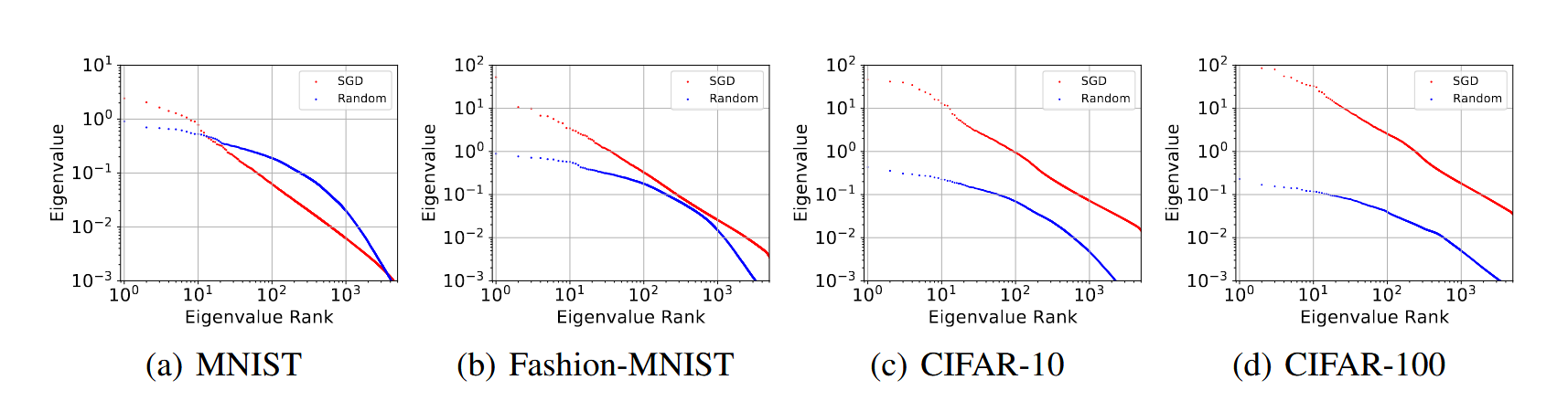
In the context of deep learning, recent work has illustrated that empirically the gradients are considerably structured and gradients are effectively live in a low-dimensional space [33, 64, 65, 29, 47], and close to convergence, almost all gradients are really close to zero, the so-called interpolation condition [13, 62, 55, 10]. Such observations have formed the basis of more memory or communication-efficient algorithms, e.g., based on top-$k$ count-sketch, truncated SGD, and heavy hitters based analysis [71, 39]. In parallel, considerable advances have been made in understanding the eigenspectrum of the Hessian [92, 87, 89, 48]. In particular, fast decaying eigenvalues have been observed across the entire range of models including ConvNets, ResNets, as well as GPT and ViT variants [92, 89], and some work [87] have empirically shown that the $k$-th largest (absolute) eigenvalue decays following power-law, i.e., $\lambda_{k}\leq\lambda_{1}k^{-s}$ with $s>\frac{1}{2}$ empirically.

We make some assumptions based on the empirically observed eigenvalue decay of the Hessian and establish bounds on the loss gradient Gaussian width based on properties of the Hessian eigenvalues.

Assumption 3.

Let $\hat{H}_{n}(\theta)=\frac{1}{n}\sum_{i=1}^{n}\nabla^{2}\ell(\theta,z_{i})$ denote the loss Hessian for $\theta\in\Theta$ and let $\bm{\lambda}(\theta)=[\lambda_{i}(\theta)],i\in[p]$ denote the (not necessarily positive) eigenvalues of $\hat{H}_{n}(\theta)$. For any $\theta\in\Theta$, the empirical gradient $\hat{\xi}_{n}(\theta)=\hat{H}_{n}(\tilde{\theta})(\theta-\theta_{0})+\hat{\xi}_{n}(\theta_{0})$ for some $\theta_{0}\in\mathbb{R}^{p},\|\theta-\theta_{0}\|_{2}\leq c$, where $\tilde{\theta}=a_{\theta}\theta+(1-a_{\theta})\theta_{0},a_{\theta}\in[0,1]$. With $\bm{\lambda}(\tilde{\theta})$ denoting the Hessian eigenvalues of $\hat{H}_{n}(\tilde{\theta})$ at any such $\tilde{\theta}$, we assume $\left\|\bm{\lambda}(\tilde{\theta})\right\|_{2}\leq\Lambda^{(u)}$ for some fixed $\Lambda^{(u)}\in\mathbb{R}_{+}$.

Remark 4.1.

Assumption 3 is inspired by the empirical evidence of Hessian eigenvalue decay especially close to convergence [92, 87], and it is reasonable to expect $\left\|\lambda(\tilde{\theta})\right\|_{2}=\tilde{O}(1)$, which means we could set $\Lambda^{(u)}=\tilde{O}(1)$. In Assumption 3, $\theta_{0}$ can be from a pretrained model or a random initialization. Further, we can replace the single $\theta_{0}$ by a set $\Theta_{0}$ of cardinality $|\Theta_{0}|=N$, so that for any $\theta\in\Theta,\exists\theta_{0}\in\Theta_{0}$ such that $\|\theta-\theta_{0}\|_{2}\leq c$, and our main result below will continue to hold with only an additional $\log N$ term [58, 17]. ∎

Theorem 4.

Under Assumption 3, the LGGW for $\theta\in\Theta$ is $w(\hat{\Xi}_{n})\leq c\Lambda^{(u)}\sqrt{\log p}$.

Remark 4.2.

The width bound in Theorem 4 depend on $\Lambda^{(u)}$, the upper bound of $\left\|\bm{\lambda}(\tilde{\theta})\right\|_{2}$, so that a power law decay of sorted absolute Hessian eigenvalues $|\lambda_{(i)}(\tilde{\theta})|\leq c^{(u)}i^{-s}$ with $s\geq\frac{1}{2}$ (e.g., as empirically observed in [87]) will lead to $\Lambda^{(u)}=O(\sqrt{\log p})$. Then, the overall bound is $w(\hat{\Xi}_{n})\leq c\log p$ yielding a generalization bound from (11) with complexity term $c\frac{\log p}{\sqrt{n}}$, hence a sharp bound. ∎

4.2 Gaussian Width Bounds for Neural Networks

Consider a training set $z^{(n)}=\{z_{i},i\in[n]\},z_{i}=(\mathbf{x}_{i},y_{i}),\mathbf{x}_{i}\in{\cal X}\subseteq\mathbb{R}^{d},y_{i}\in{\cal Y}\subseteq\mathbb{R}$. For some loss function $l$, the goal is to minimize: $\hat{\cal L}_{n}(\theta)=\frac{1}{n}\sum_{i=1}^{n}l(y_{i},\hat{y}_{i})=\frac{1}{n}\sum_{i=1}^{n}l(y_{i},f(\theta;\mathbf{x}_{i}))$, where the prediction $\hat{y}_{i}:=f(\theta;\mathbf{x}_{i})$ is from a neural network, and the parameter vector $\theta\in\mathbb{R}^{p}$. For our analysis, we will assume square loss $l(y_{i},\hat{y}_{i})=\frac{1}{2}(y_{i}-\hat{y}_{i})^{2}$, though the analyses extends to more general losses under mild additional assumptions. We focus on feedforward networks (FFNs) and residual networks (RestNets), and consider them as $L$ layer neural networks $f(\theta;\mathbf{x})$ with parameters $\theta$, where each layer has width $m$. We make two standard assumptions [1, 21, 52, 8].

Assumption 4 (Activation).

The activation function $\phi$ is 1-Lipschitz, i.e., $|\phi^{\prime}|\leq 1$ and $\phi(0)=0$.

Assumption 5 (Random initialization).

Let $\theta_{0}:=(\operatorname{vec}(W_{0}^{(1)})^{\top},\ldots,\operatorname{vec}(W_{0}^{(L)})^{\top},\mathbf{v}_{0}^{\top})^{\top}$ denote the initial weights, and $w_{0,ij}^{(l)}$ denote $i,j$-th element of weight matrix $W_{0}^{(l)}$ for $l\in[L]$. At initialization, $w_{0,ij}^{(l)}\sim{\cal N}(0,\sigma_{0}^{2})$ for $l\in[L]$ where $\sigma_{0}=\frac{\sigma_{1}}{2\left(1+\frac{\sqrt{\log m}}{\sqrt{2m}}\right)},\sigma_{1}>0$, and $\left\lVert\mathbf{v}_{0}\right\rVert_{2}=1$.

Assumption 1 is satisfied by commonly used activation functions such as (non-smooth) ReLU [2] and (smooth) GeLU [38]. The second assumption is regarding the random initialization of the weights, variants of which are typically used in most work in deep learning theory [40, 2, 37, 30, 79, 6, 22, 21].

4.2.1 Bounds for FeedForward Networks (FFNs)

We consider $f$ to be an FFN given by

$$f(\theta;x)=\mathbf{v}^{\top}\phi(\frac{1}{\sqrt{m}}W^{(L)}\phi(\cdots\phi(\frac{1}{\sqrt{m}}W^{(1)}\mathbf{x}))))~{},$$ (22)

where $W^{(1)}\in\mathbb{R}^{m\times d},W^{(l)}\in\mathbb{R}^{m\times m},l\in\{2,\ldots,L\}$ are the layer-wise weight matrices, $\mathbf{v}\in\mathbb{R}^{m}$ is the last layer vector, $\phi(\cdot)$ is the (pointwise) activation function, and the total set of parameters $\theta\in\mathbb{R}^{p},p=(L-1)m^{2}+md+m$ is given by

$\displaystyle\theta=(\operatorname{vec}(W^{(1)})^{\top},\ldots,\operatorname{vec}(W^{(L)})^{\top},\mathbf{v}^{\top})^{\top}.$ (23)

Our analysis for both FFNs and ResNets will be for gradients over all parameters in a fixed radius spectral norm ball around the initialization $\theta_{0}$, which is more flexible than Frobenius norm balls typically used in the literature [85, 19, 94, 8]:

Bρ,ρ1Spec(θ0):={θpas in (23)𝐯𝐯02ρ1,W()W0()2ρ,[L]}.assignsuperscriptsubscript𝐵𝜌subscript𝜌1Specsubscript𝜃0conditional-set𝜃superscript𝑝as in (23)formulae-sequencesubscriptnorm𝐯subscript𝐯02subscript𝜌1formulae-sequencesubscriptnormsuperscript𝑊superscriptsubscript𝑊02𝜌delimited-[]𝐿B_{\rho,\rho_{1}}^{\operatorname{Spec}}(\theta_{0}):=\big{\{}\theta\in\mathbb{R}^{p}~{}\text{as in \eqref{eq:theta_def}}~{}\mid\|\mathbf{v}-\mathbf{v}_{0}\|_{2}\leq\rho_{1},\|W^{(\ell)}-W_{0}^{(\ell)}\|_{2}\leq\rho,\ell\in[L]\big{\}}~{}. (24)

Let $B_{\rho}^{\operatorname{Spec}}(\theta_{0})\in\mathbb{R}^{p-m}$ be the corresponding set of weight matrices $W=\{W^{(l)},\ell\in[L]\}$. The main implications of our results and analyses go through as long as the layerwise spectral radius $\rho=o(\sqrt{m})$ and last layer radius $\rho_{1}=O(1)$, which are arguably practical.

Let

$\displaystyle h^{(L)}(W,\mathbf{x})$ $\displaystyle:=\phi\left(\frac{1}{\sqrt{m}}W^{(L)}\phi(\cdots\phi(\frac{1}{\sqrt{m}}W^{(1)}\mathbf{x})))\right)~{}\in\mathbb{R}^{m}$ (25)

be the “featurizer,” i.e., output of the last but one layer, so that $f(\theta;\mathbf{x})=\mathbf{v}^{\top}h^{(L)}(W,\mathbf{x})$ with $\theta=(W,\mathbf{v})$. Consider the set of all featurizer values for a single sample and as average over samples:

$\displaystyle A^{(L)}(\mathbf{x})=\left\{h^{(L)}(W,\mathbf{x})\mid W\in B_{\rho}^{\operatorname{Spec}}(\theta_{0})\right\},~{}\hat{A}_{n}^{(L)}:=\left\{\frac{1}{n}\sum_{i=1}^{n}h^{(L)}(W,\mathbf{x}_{i})\mid W\in B_{\rho}^{\operatorname{Spec}}(\theta_{0})\right\}~{}.$ (26)

We now establish an upper bound on the LGGW of FFN gradient set $\hat{\Xi}_{n}^{\operatorname{ffn}}$ corresponding to parameters in $B_{\rho,\rho_{1}}^{\operatorname{Spec}}(\theta_{0})$. In particular, we show that the LGGW can effectively be bounded by the Gaussian width of the sample average of the featurizer.

Theorem 5 (Gaussian Width of Gradients: FFNs).

Under Assumptions 4 and 5, with $\beta:=\sigma_{1}+\frac{\rho}{\sqrt{m}}$, with probability at least $\left(1-\frac{2L}{m}\right)$ over the randomness of the initialization, we have

$\displaystyle w(\hat{\Xi}_{n}^{\operatorname{ffn}})\leq c_{1}w(\hat{A}_{n}^{(L)})+c_{2}L(1+\rho_{1})\beta^{L-1}~{}.$ (27)
Remark 4.3.

Note that choosing $\sigma_{1}<1-\frac{\rho}{\sqrt{m}}$, i.e., mildly small initialization variance, satisfies $\beta<1$. When $\beta<1$, we have $w(\hat{\Xi}_{n}^{\operatorname{ffn}})=O(1)$ as long as $L=\Omega(\frac{\log(\sqrt{m}+L(1+\rho_{1}))}{\log\frac{1}{\beta}})$, which holds for moderate depth $L$. To see this, note that we have $w(\hat{\Xi}_{n}^{\operatorname{ffn}})=O(w(\hat{A}^{(L)}_{n})+L(1+\rho_{1})\beta^{L-1})$. Further, we have whp $\|\alpha^{(L)}\|_{2}\leq\beta^{L}$ (Lemma 5 in Appendix C), so that $w(\hat{A}^{(L)}_{n})\leq c\beta^{L}\sqrt{m}$. Then, for $\beta<1$, the bound $\beta^{L}\sqrt{m}+\beta^{L-1}L(1+\rho_{1})=O(1)$ if $L=\Omega(\frac{\log(\sqrt{m}+L(1+\rho_{1}))}{\log\frac{1}{\beta}})$. Interestingly, sufficient depth $L$ helps control the Gaussian width in the theoretical setting. ∎

Technicalities aside, Theorem 5 has two qualitative implications which are important to understand.

Remark 4.4.

Theorem 5 bounds the Gaussian width uniformly over all parameters in $B_{\rho,\rho_{1}}^{\operatorname{Spec}}(\theta_{0})$. Instead, we can consider the bound for parameters in $\Theta$ which are in the last 10% of the epochs of deep learning training. If the featurizer for such parameters $\theta\in\Theta$ are more stable, i.e., does not change much with changes in $W$, then the Gaussian width of the featurizer will be small. ∎

Remark 4.5.

The result implies that under suitable conditions, the Gaussian width of gradients over all $p=md+(L-1)m^{2}+m$ parameters can be reduced to the Gaussian width of the featurizer, which is $m$ dimensional. If the featurizer does feature selection, e.g., as in variants of invariant risk minimization (IRM) [5, 93] or sharpness aware minimization (SAM) [26, 4], then the Gaussian width of the featurizer will be small. On the other hand, if the featurizer has many spurious and/or random features [70, 93], then the Gaussian width will be large. ∎

Refer to caption
(a) ResNet18 on CIFAR-10
Refer to caption
(b) FFN on CIFAR-10
Refer to caption
(c) CNN on Fashion-MNIST
Figure 2: $L_{0}$ norm and $L_{1}$ norm of featurizers for (a) ResNet18 on CIFAR-10, (b) FFN on CIFAR-10, and (c) CNN on Fashion-MNIST of the last 10% epochs close to convergence. We plot both the average and maximum norms among 5 repetitions for each experiment. The figures demonstrate that for these models, as approaching convergence, the featurizers has relatively low $L_{0}$ norm and $L_{1}$ norm, which further indicates a small LGGW. All experiments are run on A100 GPUs.

4.2.2 Bounds for Residual Networks (ResNets)

We consider $f$ to be a ResNet given by

$$\begin{split}\alpha^{(l)}(\mathbf{x})&=\alpha^{(l-1)}(\mathbf{x})+\phi\left(\frac{1}{L\sqrt{m}}W^{(l)}\alpha^{(l-1)}(\mathbf{x})\right)~{},\\ f(\theta;\mathbf{x})&=\alpha^{(L+1)}(\mathbf{x})=\frac{1}{\sqrt{m}}\mathbf{v}^{\top}\alpha^{(L)}(\mathbf{x})~{},\end{split}$$ (28)

where $\alpha^{(0)}(\mathbf{x})=\mathbf{x}$, and $W^{(l)},l\in[L],\mathbf{v},\phi$ are as in FFNs. Let $h^{(L)}(W,\mathbf{x}):=\frac{1}{\sqrt{m}}\alpha^{(L)}(\mathbf{x})$ be the “featurizer,” i.e., output of the last layer, so that $f(\theta;\mathbf{x})=\mathbf{v}^{\top}h^{(L)}(W,\mathbf{x})$ with $\theta=(W,\mathbf{v})$. Note that the scaling of the residual layers is assumed to have a smaller scaling factor $\frac{1}{L}$ following standard theoretical analysis of ResNets [21] and also aligns with practice where smaller initialization variance yields state-of-the-art performance [91]. With the featurizer and associated sets defined as in (26) for FFNs, we now establish an upper bound on the LGGW of gradients in terms of that of the featurizer.

Theorem 6 (Gaussian Width of Gradients: ResNets).

Under Assumptions 4 and 5, with $\beta:=\sigma_{1}+\frac{\rho}{\sqrt{m}}$, with probability at least $\left(1-\frac{2L}{m}\right)$ over the randomness of the initialization, we have

$\displaystyle w(\hat{\Xi}_{n}^{\operatorname{rn}})\leq c_{1}w(\hat{A}_{n}^{(L)})+c_{2}(1+\rho_{1})e^{\beta}~{}.$ (29)
Remark 4.6.

As for FFNs, choosing $\sigma_{1}<1-\frac{\rho}{\sqrt{m}}$, i.e., mildly small initialization variance, satisfies $\beta<1$. When $\beta<1$, we have $w(\hat{\Xi}_{n}^{\operatorname{rn}})=O(w(\hat{A}_{n}^{(L)}))$ since $(1+\rho_{1})e^{\beta}=O(1)$. Thus, for ResNets, the Gaussian width of gradients on all parameters reduces to the Gaussian width of the featurizer. ∎

Remark 4.7.

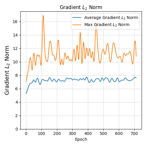
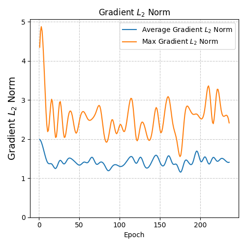
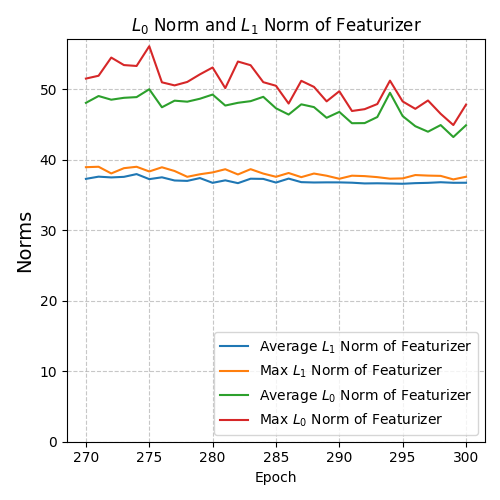
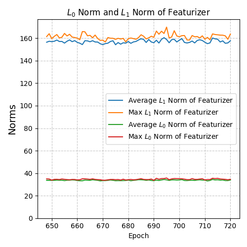
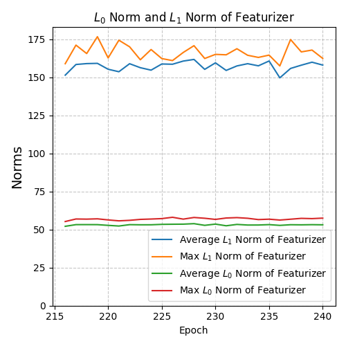
In Figure 2, we plot the average and max (over 5 runs) of the $L_{0}$ and $L_{1}$ norm of the featurizer for the last $10\%$ epochs close to convergence for three standard deep learning models: ResNet18 on CIFAR-10 (512 dimension featurizer), FFN on CIFAR-10 (256 dimension featurizer), and CNN on Fashion-MNIST (128 dimension featurizer). The small $L_{0}$ and $L_{1}$ norm of the featurizer, indicating both feature selection and being in small $L_{1}$ ball, imply small Gaussian width of the featurizer which in turn implies small LGGW based on Theorems 5 and 6. ∎

5 Conclusions

In this work, we have introduced a new approach to analyzing the generalization and optimization of learning models based on the loss gradient Gaussian width (LGGW). For loss satisfying the gradient domination condition, which includes the popular PL condition as a special case, we establish generalization bounds in terms of LGGW. In the context of optimization, we show that stochastic mini-batch gradient descent with sample reuse does not go haywire and the gradient estimates stay close to the population counterparts as long as the Gaussian width of the gradient is small. We also discuss the LGGW of deep learning models through empirical evidence, examples, and analysis of some special cases. We show that the LGGW can be bounded by the $L_{2}$ norm of the Hessian eigenvalues and the Gaussian width of the featurizer. Overall, our work demonstrates the benefits of small Gaussian width in the context of learning, and will hopefully serve as motivation for further study of this geometric perspective especially for modern learning models.

Acknowledgements.

The work was supported in part by the National Science Foundation (NSF) through awards IIS 21-31335, OAC 21-30835, DBI 20-21898, as well as a C3.ai research award.

References

  • [1] Zeyuan Allen-Zhu, Yuanzhi Li, and Zhao Song. A Convergence Theory for Deep Learning via Over-Parameterization. arXiv:1811.03962 [cs, math, stat], June 2019. arXiv: 1811.03962.
  • [2] Zeyuan Allen-Zhu, Yuanzhi Li, and Zhao Song. A convergence theory for deep learning via over-parameterization. In International conference on machine learning, pages 242–252. PMLR, 2019.
  • [3] Idan Amir, Roi Livni, and Nati Srebro. Thinking outside the ball: Optimal learning with gradient descent for generalized linear stochastic convex optimization. Advances in Neural Information Processing Systems, 35:23539–23550, 2022.
  • [4] Maksym Andriushchenko, Dara Bahri, Hossein Mobahi, and Nicolas Flammarion. Sharpness-Aware Minimization Leads to Low-Rank Features. November 2023.
  • [5] Martin Arjovsky, Léon Bottou, Ishaan Gulrajani, and David Lopez-Paz. Invariant Risk Minimization, March 2020. arXiv:1907.02893 [cs, stat].
  • [6] Sanjeev Arora, Simon Du, Wei Hu, Zhiyuan Li, and Ruosong Wang. Fine-grained analysis of optimization and generalization for overparameterized two-layer neural networks. In International Conference on Machine Learning, pages 322–332. PMLR, 2019.
  • [7] Sanjeev Arora, Simon S. Du, Wei Hu, Zhiyuan Li, Ruslan Salakhutdinov, and Ruosong Wang. On Exact Computation with an Infinitely Wide Neural Net. arXiv:1904.11955 [cs, stat], November 2019. arXiv: 1904.11955.
  • [8] A. Banerjee, P. Cisneros-Velarde, L. Zhu, and M. Belkin. Restricted strong convexity of deep learning models with smooth activations. In International Conference on Learning Representations (ICLR), 2023.
  • [9] P. L. Bartlett and S. Mendelson. Rademacher and Gaussian complexities: Risk bounds and structural results. Journal of Machine Learning Research, 3:463–482, 2002.
  • [10] Peter Bartlett. [1906.11300] Benign Overfitting in Linear Regression, 2019.
  • [11] Peter Bartlett, Dylan J. Foster, and Matus Telgarsky. Spectrally-normalized margin bounds for neural networks. arXiv:1706.08498 [cs, stat], June 2017. arXiv: 1706.08498.
  • [12] Raef Bassily, Adam Smith, and Abhradeep Thakurta. Differentially Private Empirical Risk Minimization: Efficient Algorithms and Tight Error Bounds. arXiv:1405.7085 [cs, stat], May 2014. arXiv: 1405.7085.
  • [13] Mikhail Belkin, Daniel Hsu, Siyuan Ma, and Soumik Mandal. Reconciling modern machine learning practice and the bias-variance trade-off. Proceedings of the National Academy of Sciences (PNAS), 116(32), 2019.
  • [14] Léon Bottou, Frank E. Curtis, and Jorge Nocedal. Optimization Methods for Large-Scale Machine Learning. arXiv:1606.04838 [cs, math, stat], June 2016. arXiv: 1606.04838.
  • [15] Stéphane Boucheron, Gábor Lugosi, and Pascal Massart. Concentration Inequalities: A Nonasymptotic Theory of Independence. Oxford University Press, February 2013.
  • [16] Olivier Bousquet and André Elisseeff. Stability and generalization. The Journal of Machine Learning Research, 2:499–526, 2002.
  • [17] Sheng Chen and Arindam Banerjee. Structured estimation with atomic norms: General bounds and applications. In Advances in Neural Information Processing Systems 28, 2015.
  • [18] Sheng Chen and Arindam Banerjee. An improved analysis of alternating minimization for structured multi-response regression. In Advances in Neural Information Processing Systems (NeurIPS), 2018.
  • [19] Lénaïc Chizat, Edouard Oyallon, and Francis Bach. On Lazy Training in Differentiable Programming. page 11.
  • [20] Damek Davis and Dmitriy Drusvyatskiy. Graphical convergence of subgradients in nonconvex optimization and learning. Mathematics of Operations Research, 47(1):209–231, 2022.
  • [21] Simon S. Du, Jason D. Lee, Haochuan Li, Liwei Wang, and Xiyu Zhai. Gradient Descent Finds Global Minima of Deep Neural Networks. International Conference on Machine Learning (ICML), November 2019. arXiv: 1811.03804.
  • [22] Simon S Du, Xiyu Zhai, Barnabas Poczos, and Aarti Singh. Gradient descent provably optimizes over-parameterized neural networks. In International Conference on Learning Representations, 2018.
  • [23] Cynthia Dwork, Vitaly Feldman, Moritz Hardt, Toniann Pitassi, Omer Reingold, and Aaron Roth. Generalization in Adaptive Data Analysis and Holdout Reuse. arXiv:1506.02629 [cs], June 2015. arXiv: 1506.02629.
  • [24] Cynthia Dwork, Vitaly Feldman, Moritz Hardt, Toniann Pitassi, Omer Reingold, and Aaron Leon Roth. Preserving statistical validity in adaptive data analysis. In Rocco A. Servedio and Ronitt Rubinfeld, editors, Proceedings of the Forty-Seventh Annual ACM on Symposium on Theory of Computing, STOC 2015, Portland, OR, USA, June 14-17, 2015, pages 117–126. ACM, 2015.
  • [25] Pierre Foret, Ariel Kleiner, Hossein Mobahi, and Behnam Neyshabur. Sharpness-aware minimization for efficiently improving generalization. In International Conference on Learning Representations, 2020.
  • [26] Pierre Foret, Ariel Kleiner, Hossein Mobahi, and Behnam Neyshabur. Sharpness-Aware Minimization for Efficiently Improving Generalization, April 2021. arXiv:2010.01412 [cs, stat].
  • [27] Dylan J. Foster, Ayush Sekhari, and Karthik Sridharan. Uniform convergence of gradients for non-convex learning and optimization. In Proceedings of the 32nd International Conference on Neural Information Processing Systems, NIPS’18, 2018.
  • [28] S. Ghadimi and G. Lan. Optimal Stochastic Approximation Algorithms for Strongly Convex Stochastic Composite Optimization I: A Generic Algorithmic Framework. SIAM Journal on Optimization, 22(4):1469–1492, January 2012.
  • [29] Behrooz Ghorbani, Shankar Krishnan, and Ying Xiao. An Investigation into Neural Net Optimization via Hessian Eigenvalue Density. arXiv:1901.10159 [cs, stat], January 2019. arXiv: 1901.10159.
  • [30] Xavier Glorot and Yoshua Bengio. Understanding the difficulty of training deep feedforward neural networks. In Proceedings of the Thirteenth International Conference on Artificial Intelligence and Statistics, 2010.
  • [31] Noah Golowich, Alexander Rakhlin, and Ohad Shamir. Size-Independent Sample Complexity of Neural Networks. arXiv:1712.06541 [cs, stat], December 2017. arXiv: 1712.06541.
  • [32] Ian Goodfellow, Yoshua Bengio, and Aaron Courville. Deep Learning. MIT Press, 2016.
  • [33] Guy Gur-Ari, Daniel A. Roberts, and Ethan Dyer. Gradient Descent Happens in a Tiny Subspace. September 2018.
  • [34] Jeff Haochen and Suvrit Sra. Random shuffling beats sgd after finite epochs. In International Conference on Machine Learning, pages 2624–2633. PMLR, 2019.
  • [35] Jeffery Z. HaoChen and Suvrit Sra. Random Shuffling Beats SGD after Finite Epochs. arXiv:1806.10077 [math, stat], June 2018. arXiv: 1806.10077.
  • [36] Moritz Hardt, Ben Recht, and Yoram Singer. Train faster, generalize better: Stability of stochastic gradient descent. In International conference on machine learning, pages 1225–1234. PMLR, 2016.
  • [37] Kaiming He, Xiangyu Zhang, Shaoqing Ren, and Jian Sun. Delving deep into rectifiers: Surpassing human-level performance on imagenet classification. In Proceedings of the IEEE International Conference on Computer Vision, 2015.
  • [38] Dan Hendrycks and Kevin Gimpel. Gaussian error linear units (gelus). arXiv preprint arXiv:1606.08415, 2016.
  • [39] Nikita Ivkin, Daniel Rothchild, Enayat Ullah, Ion Stoica, Raman Arora, et al. Communication-efficient distributed sgd with sketching. Advances in Neural Information Processing Systems, 32, 2019.
  • [40] Arthur Jacot, Franck Gabriel, and Clément Hongler. Neural Tangent Kernel: Convergence and Generalization in Neural Networks. arXiv:1806.07572 [cs, math, stat], February 2020. arXiv: 1806.07572.
  • [41] Christopher Jung, Katrina Ligett, Seth Neel, Aaron Roth, Saeed Sharifi-Malvajerdi, and Moshe Shenfeld. A new analysis of differential privacy’s generalization guarantees. In Thomas Vidick, editor, 11th Innovations in Theoretical Computer Science Conference, ITCS 2020, January 12-14, 2020, Seattle, Washington, USA, volume 151 of LIPIcs, pages 31:1–31:17. Schloss Dagstuhl - Leibniz-Zentrum für Informatik, 2020.
  • [42] Sham M. Kakade, Shai Shalev-Shwartz, and Ambuj Tewari. Regularization techniques for learning with matrices. J. Mach. Learn. Res., 13:1865–1890, 2012.
  • [43] Sham M. Kakade, Karthik Sridharan, and Ambuj Tewari. On the complexity of linear prediction: Risk bounds, margin bounds, and regularization. In NIPS, 2009.
  • [44] V. Koltchinskii and D. Panchenko. Rademacher processes and bounding the risk of function learning. High Dimensional Probability II, pages 443–457, 2000.
  • [45] Yann LeCun, Yoshua Bengio, and Geoffrey Hinton. Deep learning. Nature, 521(7553):436–444, May 2015.
  • [46] M. Ledaux and M. Talagrand. Probability in Banach Spaces: Isometry and Processes. Springer, 1991.
  • [47] Xinyan Li, Qilong Gu, Yingxue Zhou, Tiancong Chen, and Arindam Banerjee. Hessian based analysis of SGD for deep nets: Dynamics and generalization. In SIAM International Conference on Data Mining, (SDM), pages 190–198, 2020.
  • [48] Xinyan Li, Qilong Gu, Yingxue Zhou, Tiancong Chen, and Arindam Banerjee. Hessian based analysis of sgd for deep nets: Dynamics and generalization. In Proceedings of the 2020 SIAM International Conference on Data Mining, pages 190–198. SIAM, 2020.
  • [49] C. Liu, L. Zhu, and M. Belkin. Loss landscapes and optimization in over-parameterized non-linear systems and neural networks. Applied and Computational Harmonic Analysis, 59:85–116, 2022.
  • [50] Chaoyue Liu, Libin Zhu, and Mikhail Belkin. Toward a theory of optimization for over-parameterized systems of non-linear equations: the lessons of deep learning. arXiv:2003.00307 [cs, math, stat], February 2020. arXiv: 2003.00307.
  • [51] Chaoyue Liu, Libin Zhu, and Mikhail Belkin. Loss landscapes and optimization in over-parameterized non-linear systems and neural networks. arXiv:2003.00307 [cs, math, stat], May 2021. arXiv: 2003.00307.
  • [52] Chaoyue Liu, Libin Zhu, and Mikhail Belkin. On the linearity of large non-linear models: when and why the tangent kernel is constant. arXiv:2010.01092 [cs, stat], February 2021. arXiv: 2010.01092.
  • [53] Chaoyue Liu, Libin Zhu, and Misha Belkin. On the linearity of large non-linear models: when and why the tangent kernel is constant. In Advances in Neural Information Processing Systems, 2020.
  • [54] Yucheng Lu, Si Yi Meng, and Christopher De Sa. A general analysis of example-selection for stochastic gradient descent. In International Conference on Learning Representations, 2022.
  • [55] Siyuan Ma, Raef Bassily, and Mikhail Belkin. The Power of Interpolation: Understanding the Effectiveness of SGD in Modern Over-parametrized Learning. arXiv:1712.06559 [cs, stat], December 2017. arXiv: 1712.06559.
  • [56] Andreas Maurer. A vector-contraction inequality for rademacher complexities. In Algorithmic Learning Theory (ALT), volume 9925, pages 3–17, 2016.
  • [57] Andreas Maurer and Massimiliano Pontil. Bounds for vector-valued function estimation. arXiv, abs/1606.01487, 2016.
  • [58] Andreas Maurer, Massimiliano Pontil, and Bernardino Romera-Paredes. An Inequality with Applications to Structured Sparsity and Multitask Dictionary Learning. arXiv:1402.1864 [cs, stat], February 2014. arXiv: 1402.1864.
  • [59] Song Mei, Yu Bai, and Andrea Montanari. The landscape of empirical risk for nonconvex losses. The Annals of Statistics, 46(6A):2747–2774, 2018.
  • [60] Mehryar Mohri, Afshin Rostamizadeh, and Ameet Talwalkar. Foundations of Machine Learning. MIT Press, 2018.
  • [61] Vaishnavh Nagarajan and J. Zico Kolter. Uniform convergence may be unable to explain generalization in deep learning. arXiv:1902.04742 [cs, stat], December 2019. arXiv: 1902.04742.
  • [62] Jeffrey Negrea, Gintare Karolina Dziugaite, and Daniel M. Roy. In Defense of Uniform Convergence: Generalization via derandomization with an application to interpolating predictors. arXiv:1912.04265 [cs, stat], December 2019. arXiv: 1912.04265.
  • [63] A. Nemirovski, A. Juditsky, G. Lan, and A. Shapiro. Robust Stochastic Approximation Approach to Stochastic Programming. SIAM Journal on Optimization, 19(4):1574–1609, January 2009.
  • [64] Vardan Papyan. The Full Spectrum of Deepnet Hessians at Scale: Dynamics with SGD Training and Sample Size. arXiv:1811.07062 [cs, stat], November 2018. arXiv: 1811.07062.
  • [65] Vardan Papyan. Measurements of three-level hierarchical structure in the outliers in the spectrum of deepnet hessians. In International Conference on Machine Learning, pages 5012–5021. PMLR, 2019.
  • [66] Boris Polyak. Gradient methods for the minimisation of functionals. Ussr Computational Mathematics and Mathematical Physics, 3:864–878, 12 1963.
  • [67] Shashank Rajput, Anant Gupta, and Dimitris Papailiopoulos. Closing the convergence gap of SGD without replacement. In Hal Daumé III and Aarti Singh, editors, Proceedings of the 37th International Conference on Machine Learning, volume 119 of Proceedings of Machine Learning Research, pages 7964–7973. PMLR, 13–18 Jul 2020.
  • [68] Benjamin Recht and Christopher Re. Beneath the valley of the noncommutative arithmetic-geometric mean inequality: conjectures, case-studies, and consequences. arXiv:1202.4184 [math, stat], February 2012. arXiv: 1202.4184.
  • [69] Sashank J Reddi, Satyen Kale, and Sanjiv Kumar. ON THE CONVERGENCE OF ADAM AND BEYOND. page 23, 2018.
  • [70] Elan Rosenfeld, Pradeep Ravikumar, and Andrej Risteski. The Risks of Invariant Risk Minimization, March 2021. arXiv:2010.05761 [cs, stat].
  • [71] Daniel Rothchild, Ashwinee Panda, Enayat Ullah, Nikita Ivkin, Ion Stoica, Vladimir Braverman, Joseph Gonzalez, and Raman Arora. Fetchsgd: Communication-efficient federated learning with sketching. In International Conference on Machine Learning, pages 8253–8265. PMLR, 2020.
  • [72] Itay Safran and Ohad Shamir. How good is sgd with random shuffling? In Conference on Learning Theory, pages 3250–3284. PMLR, 2020.
  • [73] Shai Shalev-Shwartz and Shai Ben-David. Understanding machine learning: From theory to algorithms. Cambridge University Press, 2014.
  • [74] Shai Shalev-Shwartz, Ohad Shamir, Nathan Srebro, and Karthik Sridharan. Stochastic Convex Optimization. page 9, 2009.
  • [75] Shai Shalev-Shwartz, Ohad Shamir, Nathan Srebro, and Karthik Sridharan. Learnability, Stability and Uniform Convergence. Journal of Machine Learning Research, 11(Oct):2635–2670, 2010.
  • [76] Ohad Shamir. Without-Replacement Sampling for Stochastic Gradient Methods. In D. D. Lee, M. Sugiyama, U. V. Luxburg, I. Guyon, and R. Garnett, editors, Advances in Neural Information Processing Systems 29, pages 46–54. Curran Associates, Inc., 2016.
  • [77] Lorenzo De Stefani and Eli Upfal. A rademacher complexity based method for controlling power and confidence level in adaptive statistical analysis. In IEEE International Conference on Data Science and Advanced Analytics, DSAA. IEEE, 2019.
  • [78] Thomas Steinke and Jonathan Ullman. Interactive fingerprinting codes and the hardness of preventing false discovery. In 2016 Information Theory and Applications Workshop, ITA 2016, La Jolla, CA, USA, January 31 - February 5, 2016, pages 1–41. IEEE, 2016.
  • [79] Ilya Sutskever, James Martens, George Dahl, and Geoffrey Hinton. On the importance of initialization and momentum in deep learning. In Proceedings of the 30th International Conference on Machine Learning, 2013.
  • [80] M. Talagrand. Upper and Lower Bounds for Stochastic Processes. Springer, 2014.
  • [81] Michel Talagrand. Majorizing measures: the generic chaining. The Annals of Probability, 24(3):1049–1103, July 1996.
  • [82] R. Vershynin. Introduction to the non-asymptotic analysis of random matrices. In Y. Eldar and G. Kutyniok, editors, Compressed Sensing, chapter 5, pages 210–268. Cambridge University Press, 2012.
  • [83] Roman Vershynin. High-Dimensional Probability. page 301, 2018.
  • [84] Roman Vershynin. High-Dimensional Probability: An Introduction with Applications in Data Science. Cambridge Series in Statistical and Probabilistic Mathematics. Cambridge University Press, 2018.
  • [85] Blake Woodworth, Suriya Gunasekar, Jason D. Lee, Edward Moroshko, Pedro Savarese, Itay Golan, Daniel Soudry, and Nathan Srebro. Kernel and Rich Regimes in Overparametrized Models. arXiv:2002.09277 [cs, stat], February 2020. arXiv: 2002.09277.
  • [86] Yikai Wu, Xingyu Zhu, Chenwei Wu, Annie Wang, and Rong Ge. Dissecting hessian: Understanding common structure of hessian in neural networks. arXiv preprint arXiv:2010.04261, 2022.
  • [87] Zeke Xie, Qian-Yuan Tang, Yunfeng Cai, Mingming Sun, and Ping Li. On the Power-Law Hessian Spectrums in Deep Learning, August 2022. arXiv:2201.13011 [physics, q-bio].
  • [88] Zeke Xie, Qian-Yuan Tang, Zheng He, Mingming Sun, and Ping Li. Rethinking the structure of stochastic gradients: Empirical and statistical evidence. arXiv preprint arXiv:2212.02083, 2022.
  • [89] Zhewei Yao, Amir Gholami, Kurt Keutzer, and Michael Mahoney. PyHessian: Neural Networks Through the Lens of the Hessian, March 2020. arXiv:1912.07145 [cs, math].
  • [90] Manzil Zaheer, Sashank Reddi, Devendra Sachan, Satyen Kale, and Sanjiv Kumar. Adaptive Methods for Nonconvex Optimization. In S. Bengio, H. Wallach, H. Larochelle, K. Grauman, N. Cesa-Bianchi, and R. Garnett, editors, Advances in Neural Information Processing Systems 31, pages 9793–9803. Curran Associates, Inc., 2018.
  • [91] Chiyuan Zhang, Samy Bengio, Moritz Hardt, Benjamin Recht, and Oriol Vinyals. Understanding deep learning requires rethinking generalization. arXiv:1611.03530 [cs], February 2017. arXiv: 1611.03530.
  • [92] Yushun Zhang, Congliang Chen, Tian Ding, Ziniu Li, Ruoyu Sun, and Zhi-Quan Luo. Why Transformers Need Adam: A Hessian Perspective, February 2024. arXiv:2402.16788 [cs].
  • [93] Xiao Zhou, Yong Lin, Weizhong Zhang, and Tong Zhang. Sparse Invariant Risk Minimization. In Proceedings of the 39th International Conference on Machine Learning, pages 27222–27244. PMLR, June 2022. ISSN: 2640-3498.
  • [94] Difan Zou, Yuan Cao, Dongruo Zhou, and Quanquan Gu. Stochastic Gradient Descent Optimizes Over-parameterized Deep ReLU Networks. arXiv:1811.08888 [cs, math, stat], November 2018. arXiv: 1811.08888.

Appendix A Generalization Bounds: Proofs for Section 2

In this section, we provide proofs for results in Section 2.

A.1 Generalization bound in terms NERC, following [27]

Proof sketch of Main Result

We start with a variation of Proposition 1 of [27], which will be convenient for our purposes.

Proposition 2.

Under Assumptions 1 and 2, with $\theta^{\star}\in\arg\min_{\theta\in\Theta}L_{\mathcal{D}}(w)$ denoting any population loss minimizer and $\hat{R}_{n}(\hat{\Xi}^{(n)})$ as in Definition 3, for any $\delta>0$, with probability at least $1-\delta$ over the draw of the samples $z^{(n)}\sim{\cal D}^{n}$, for any $\hat{\theta}\in\Theta$ we have

$\displaystyle{\cal L}_{{\cal D}}(\hat{\theta})-{\cal L}(\theta^{*})\leq 2c_{0}\left(\|\nabla\hat{{\cal L}}_{n}(\hat{\theta})\|^{\alpha}+2\left(\mathbb{E}\sup_{\theta\in\Theta}\|\nabla\hat{{\cal L}}_{n}(\theta)-\nabla{\cal L}_{D}(\theta)\|\right)^{\alpha}+c_{2}\left(\frac{\log\frac{1}{\delta}}{n}\right)^{\frac{\alpha}{2}}\right)~{}.$ (30)
Proof.

Since ${\cal L}_{{\cal D}}$ satisfies the $(\alpha,c_{0})$-GD condition, since $\alpha\in[1,2]$, we have

$\displaystyle{\cal L}_{{\cal D}}(\hat{\theta})-{\cal L}(\theta^{*})$ $\displaystyle\leq c_{0}\|\nabla{\cal L}_{{\cal D}}(\hat{\theta})\|^{\alpha}\leq 2c_{0}\left(\|\nabla\hat{{\cal L}}_{n}(\hat{\theta})\|^{\alpha}+\|\nabla\hat{{\cal L}}_{n}(\hat{\theta})-\nabla{\cal L}_{{\cal D}}(\hat{\theta})\|^{\alpha}\right)$
$\displaystyle\leq 2c_{0}\left(\|\nabla\hat{{\cal L}}_{n}(\hat{\theta})\|^{\alpha}+\left(\sup_{\theta\in\Theta}\|\nabla\hat{{\cal L}}_{n}(\theta)-\nabla{\cal L}_{{\cal D}}(\theta)\|\right)^{\alpha}\right)$

Now, by a direct application of McDiarmid’s inequality, since $z^{(n)}\sim{\cal D}^{n}$, with probability at least $(1-\delta)$ over the draw of $z^{(n)}$, we have

$\displaystyle\sup_{\theta\in\Theta}~{}\left\|\frac{1}{n}\sum_{i=1}^{n}\nabla\ell(\theta;z_{i})-\mathbb{E}_{z}[\nabla\ell(\theta;z)]\right\|\leq\mathbb{E}\sup_{\theta\in\Theta}\left\|\frac{1}{n}\sum_{i=1}^{n}\nabla\ell(\theta;z_{i})-\mathbb{E}_{z}[\nabla\ell(\theta;z)]\right\|+c\sup_{\begin{subarray}{c}\theta\in\Theta\\ z\in{\cal Z}\end{subarray}}\|\nabla\ell(\theta;z)\|\sqrt{\frac{\log\frac{1}{\delta}}{n}}~{}.$

Noting that $\|\nabla\ell(\theta;z)\|_{2}=O(1)$ for $\theta\in\Theta,z\in{\cal Z}$ completes the proof. ∎

Next, we effectively restate Proposition 2 of [27], in our notation.

Proposition 3.

Let $\hat{\Xi}^{(n)}$ be the set of all $n$-tuple gradients as in (2) and $\hat{R}_{n}(\hat{\Xi}^{(n)})$ be the NERC (normed empirical Rademacher complexity) as in Definition 3. For any $\delta>0$, with probability at least $1-\delta$ over the draw of $z^{(n)}\sim{\cal D}^{n}$, we have

$$\mathbb{E}\sup_{\theta\in\Theta}\left\|\nabla\widehat{L}_{n}(\theta)-\nabla L_{\mathcal{D}}(\theta)\right\|\leq 4\cdot\hat{R}_{n}(\hat{\Xi}^{(n)})+c_{1}\left(\frac{\log\left(\frac{1}{\delta}\right)}{n}\right)~{}.$$ (31)
Proof.

The proof follows from that of Proposition 2 of [27]. ∎

Combining Propositions 2 and 3, we now get the following result. See 1

A.2 Bounding NERC with Gaussian width

See 1

We establish the result by an application of the entropy method, and the specific application is just the bounded difference inequality [15]. Recall that a function $f:{\cal X}^{n}\mapsto\mathbb{R}$ is said to have the bounded difference property is for some non-negative constants $c_{1},\ldots,c_{n}$, we have for $1\leq i\leq n$

$$\sup_{\begin{subarray}{c}x_{1},\ldots,x_{n}\\ x_{i}^{\prime}\in{\cal X}\end{subarray}}~{}|f(x_{1},\ldots,x_{n})-f(x_{1},\ldots,x_{i-1},x_{i}^{\prime},x_{i+1},\ldots,x_{n})|\leq c_{i}~{}.$$ (32)

If $f$ satisfies the bounded difference property, then an application of the Efron-Stein inequality [15][Theorem 3.1] implies that $Z=f(X_{1},\ldots,X_{n})$ satisfies the variance $\text{var}(Z)\leq\frac{1}{4}\sum_{i=1}^{n}c_{i}^{2}$ [15][Corollary 3.2]. The bounded difference inequality is an application of the entropy method [15][Theorem 6.2] which shows that such $Z$ satisfies a sub-Gaussian tail inequality where the role of the sub-Gaussian norm [82, 84] is played by the variance $v=\frac{1}{4}\sum_{i}c_{i}^{2}$, so that

$$\mathbb{P}(|Z-\mathbb{E}[Z]|>u)\leq 2\exp(-u^{2}/2v)~{}.$$ (33)

We now focus on the specific result we need and prove it using the bounded difference inequality.

Proof.

Since $\mathbf{v}_{i}$ are fixed, let

$\displaystyle f(\varepsilon_{i},\ldots,\varepsilon_{n}):=\left\|\frac{1}{\sqrt{n}}\sum_{i=1}^{n}\varepsilon_{i}\mathbf{v}_{i}\right\|_{2}~{}.$

By triangle inequality, for any $j\in\{1,\ldots,n\}$, we have

$\displaystyle\sup_{\begin{subarray}{c}\varepsilon_{1},\ldots,\varepsilon_{n}\\ \varepsilon_{j}^{\prime}\in\{-1,+1\}\end{subarray}}$ $\displaystyle~{}|f(\varepsilon_{1},\ldots,\varepsilon_{n})-f(\varepsilon_{1},\ldots,\varepsilon_{j-1},\varepsilon_{j}^{\prime},\varepsilon_{j+1},\ldots,\varepsilon_{n})|$
$\displaystyle\leq\sup_{\begin{subarray}{c}\varepsilon_{1},\ldots,\varepsilon_{n}\\ \varepsilon_{j}^{\prime}\in\{-1,+1\}\end{subarray}}~{}\left|\left\|\frac{1}{\sqrt{n}}\sum_{i=1}^{n}\varepsilon_{i}\mathbf{v}_{i}\right\|_{2}-\left\|\frac{1}{\sqrt{n}}\left(\sum_{i=1}^{n}\varepsilon_{i}\mathbf{v}_{i}-\varepsilon_{j}\mathbf{v}_{j}+\varepsilon_{j}^{\prime}\mathbf{v}_{j}\right)\right\|_{2}\right|$
$\displaystyle\leq\sup_{\varepsilon_{j},\varepsilon_{j}^{\prime}\in\{-1,+1\}}\frac{1}{\sqrt{n}}\left\|\varepsilon_{j}\mathbf{v}_{j}-\varepsilon_{j}^{\prime}\mathbf{v}_{j}\right\|_{2}$
$\displaystyle\leq\frac{2}{\sqrt{n}}\|\mathbf{v}_{j}\|_{2}~{}.$

As a result, the varinace bound $v=\frac{1}{4}\sum_{i=1}^{n}\frac{2^{2}}{n}\|\mathbf{v}_{i}\|_{2}^{2}\leq 1$, since $\sum_{i=1}^{n}\|\mathbf{v}_{i}\|^{2}_{2}\leq n$.

Further, we have $\mathbb{E}[f(\varepsilon_{1},\ldots,\varepsilon_{n})]\leq 1$. To see this, first note that

$\displaystyle\mathbb{E}[f^{2}(\varepsilon_{1},\ldots,\varepsilon_{n})]=\mathbb{E}\left[\left\|\frac{1}{\sqrt{n}}\sum_{i=1}^{n}\varepsilon_{i}\mathbf{v}_{i}\right\|_{2}^{2}\right]=\frac{1}{n}\mathbb{E}\left[\sum_{i=1}^{n}\|\mathbf{v}_{i}\|_{2}^{2}+\sum_{\begin{subarray}{c}i,j=1\\ i\neq j\end{subarray}}^{n}\langle\varepsilon_{i}\mathbf{v}_{i},\varepsilon_{j}\mathbf{v}_{j}\rangle\right]\overset{(a)}{\leq}1$

where $(a)$ follows since $\sum_{i=1}^{n}\|\mathbf{v}_{i}\|^{2}_{2}\leq n$ and by independence, for $i\neq j$, $\mathbb{E}[\langle\varepsilon_{i}\mathbf{v}_{i},\varepsilon_{j}\mathbf{v}_{j}\rangle]=\langle\mathbb{E}[\varepsilon_{i}\mathbf{v}_{i}],\mathbb{E}[\varepsilon_{j}\mathbf{v}_{j}]\rangle=0$ since $\mathbb{E}[\varepsilon_{i}]=0$. Then, by Jensen’s inequality, we have

$\displaystyle\mathbb{E}[f((\varepsilon_{1},\ldots,\varepsilon_{n})]$ $\displaystyle=\mathbb{E}\left[\left\|\frac{1}{\sqrt{n}}\sum_{i=1}^{n}\varepsilon_{i}\mathbf{v}_{i}\right\|_{2}\right]\leq\sqrt{\mathbb{E}\left[\left\|\frac{1}{\sqrt{n}}\sum_{i=1}^{n}\varepsilon_{i}\mathbf{v}_{i}\right\|_{2}^{2}\right]}\leq 1~{}.$

Then, an application of the bounded difference inequality (33[15][Theorem 6.2] completes the proof. ∎

Next we focus on the proof of Lemma 20. The proof follows the standard generic chaining analysis [80] with suitable adjustments to handle the constant shift $\mu$.

See 2

Proof.

We consider an optimal admissible sequence $\{\Gamma^{(n)}_{r}\}$, i.e., sequence of subsets $\Gamma^{(n)}_{r}$ of  $\hat{\Xi}^{(n)}$ with $|\Gamma^{(n)}_{r}|\leq N_{r}$, where $N_{0}=1,N_{r}=2^{2^{r}}\text{ if }r\geq 1$, and

$\displaystyle\gamma_{2}(\hat{\Xi}^{(n)},\bar{d}^{(n)})=\sup_{\hat{\xi}^{(n)}\in\hat{\Xi}^{(n)}}\sum_{r\geq 0}2^{r/2}\bar{d}^{(n)}(\hat{\Xi}^{(n)},\Gamma^{(n)}_{r})~{}.$ (34)

For any $\hat{\xi}^{(n)}\in\hat{\Xi}^{(n)}$, let $\pi_{r}(\hat{\xi}^{(n)})\in\Gamma^{(n)}_{r}$ be the ”projection” of $\hat{\xi}^{(n)}$ to $\Gamma^{(n)}_{r}$, i.e.,

$\displaystyle\pi_{r}(\hat{\xi}^{(n)})=\underset{\hat{\xi}^{(n)}_{r}\in\Gamma^{(n)}_{r}}{\operatorname{argmin}}~{}\bar{d}^{(n)}(\hat{\xi}^{(n)},\hat{\xi}^{(n)}_{r})~{}.$ (35)

Further, let $\hat{\xi}^{(n)}_{0}\in\hat{\Xi}^{(n)}$ be such that $X_{\hat{\xi}^{(n)}_{0}}=0$. For any $\hat{\xi}^{(n)}\in\hat{\Xi}^{(n)}$, we can decompose $X_{\hat{\xi}^{(n)}}$ as

$\displaystyle X_{\hat{\xi}^{(n)}}=\sum_{r\geq 1}\left(X_{\pi_{r}(\hat{\xi}^{(n)})}-X_{\pi_{r-1}(\hat{\xi}^{(n)})}\right)+X_{\hat{\xi}^{(n)}_{0}}~{},$ (36)

which holds provided we have chosen the sequence of sets $\{\Gamma^{(n)}_{r}\}$ such that $\pi_{R}(\hat{\xi}^{(n)})=\hat{\xi}^{(n)}$ for $R$ large enough. Now, based on the shifted increment condition (19), for any $u>0$, we have

$\displaystyle\mathbb{P}(\left|X_{\pi_{r}(\hat{\xi}^{(n)})}-X_{\pi_{r-1}(\hat{\xi}^{(n)})}\right|>c_{0}(\mu+u2^{r/2})\bar{d}^{(n)}(\pi_{r}(\hat{\xi}^{(n)}),\pi_{r-1}(\hat{\xi}^{(n)}))\leq c_{1}\exp(-u^{2}2^{r}/2)~{}.$ (37)

Over all $\hat{\xi}^{(n)}\in\hat{\Xi}^{(n)}$, the number of possible pairs $\left(\pi_{r}(\hat{\xi}^{(n)}),\pi_{r-1}(\hat{\xi}^{(n)})\right)$ is

$$|\Gamma^{(n)}_{r}|\cdot|\Gamma^{(n)}_{r-1}|\leq N_{r}N_{r-1}\leq N_{r+1}=2^{2^{r+1}}~{}.$$

Applying union bound over all the possible pairs of $\left(\pi_{r}(\hat{\xi}^{(n)}),\pi_{r-1}(\hat{\xi}^{(n)})\right)$, we have

$\displaystyle\forall r\geq 1,\forall\hat{\xi}^{(n)}\in\hat{\Xi}^{(n)},\qquad\left|X_{\pi_{r}(\hat{\xi}^{(n)})}-X_{\pi_{r-1}(\hat{\xi}^{(n)})}\right|\leq c_{0}(\mu+u2^{r/2})\bar{d}^{(n)}(\pi_{r}(\hat{\xi}^{(n)}),\pi_{r-1}(\hat{\xi}^{(n)}))$ (38)

with probability at least

$\displaystyle 1-\sum_{r\geq 1}2^{2^{r+1}}\cdot c_{1}\exp(-u^{2}2^{r}/2)\geq 1-c_{3}\exp(-u^{2}/2)~{},$ (39)

where $c_{3}$ is a positive constant. From (36), (38), and (39), using the fact that $X_{\hat{\xi}^{(n)}_{0}}=0$, we have

$\displaystyle\mathbb{P}$ $\displaystyle\left(\sup_{\hat{\xi}^{(n)}\in\hat{\Xi}^{(n)}}~{}\left|X_{\hat{\xi}^{(n)}}\right|>\sup_{\hat{\xi}^{(n)}\in\hat{\Xi}^{(n)}}\sum_{r\geq 1}c_{0}(\mu+u2^{r/2})\bar{d}^{(n)}(\pi_{r}(\hat{\xi}^{(n)}),\pi_{r-1}(\hat{\xi}^{(n)}))\right)\leq c_{3}\exp\left(-\frac{u^{2}}{2}\right)~{}.$

By triangle inequality, we have

$\displaystyle\bar{d}^{(n)}(\pi_{r}(\hat{\xi}^{(n)}),\pi_{r-1}(\hat{\xi}^{(n)}))\leq\bar{d}^{(n)}(\hat{\xi}^{(n)},\pi_{r}(\hat{\xi}^{(n)}))+\bar{d}^{(n)}(\hat{\xi}^{(n)},\pi_{r-1}(\hat{\xi}^{(n)}))~{},$

so that

$\displaystyle\sup_{\hat{\xi}^{(n)}\in\hat{\Xi}^{(n)}}\sum_{r\geq 1}(\mu+u2^{r/2})\bar{d}^{(n)}(\pi_{r}(\hat{\xi}^{(n)}),\pi_{r-1}(\hat{\xi}^{(n)}))$ $\displaystyle\leq\sup_{\hat{\xi}^{(n)}\in\hat{\Xi}^{(n)}}2\sum_{r\geq 0}(\mu+u2^{r/2})\bar{d}^{(n)}(\hat{\xi}^{(n)},\pi_{r}(\hat{\xi}^{(n)}))$
$\displaystyle\leq 2(\mu+u)\sup_{\hat{\xi}^{(n)}\in\hat{\Xi}^{(n)}}\sum_{r\geq 0}2^{r/2}\bar{d}^{(n)}(\hat{\xi}^{(n)},\pi_{r}(\hat{\xi}^{(n)}))$
$\displaystyle\leq 2(\mu+u)\gamma_{2}(\hat{\Xi}^{(n)},\bar{d}^{(n)})~{}.$

As a result, we have

$\displaystyle\mathrm{P}\left(\sup_{\hat{\xi}^{(n)}\in\hat{\Xi}^{(n)}}\left|X_{\hat{\xi}^{(n)}}\right|>2c_{0}(\mu+u)\gamma_{2}(\hat{\Xi}^{(n)},\bar{d}^{(n)})\right)\leq c_{3}\exp\left(-\frac{u^{2}}{2}\right).$ (40)

That completes the proof. ∎

Using Lemma 1 and 20, we can now prove Theorem 1.

See 1

Proof.

For any $\hat{\xi}^{(n)}_{1},\hat{\xi}^{(n)}_{2}\in\hat{\Xi}^{(n)}$, for any $u>0$, by triangle inequality,

$\displaystyle\mathbb{P}_{\varepsilon^{(n)}}$ $\displaystyle\left(\left\|\frac{1}{\sqrt{n}}\sum_{i=1}^{n}\varepsilon_{i}\xi_{i,1}\right\|_{2}-\left\|\frac{1}{\sqrt{n}}\sum_{i=1}^{n}\varepsilon_{i}\xi_{i,2}\right\|_{2}\geq u\bar{d}^{(n)}(\hat{\xi}_{1}^{(n)},\hat{\xi}_{2}^{(n)})\right)\leq\mathbb{P}_{\varepsilon^{(n)}}\left(\left\|\frac{1}{\sqrt{n}}\sum_{i=1}^{n}\varepsilon_{i}(\xi_{i,1}-\xi_{i,2})\right\|_{2}\geq u\bar{d}^{(n)}(\hat{\xi}_{1}^{(n)},\hat{\xi}_{2}^{(n)})\right)~{}.$

Similarly,

$\displaystyle\mathbb{P}_{\varepsilon^{(n)}}$ $\displaystyle\left(\left\|\frac{1}{\sqrt{n}}\sum_{i=1}^{n}\varepsilon_{i}\xi_{i,2}\right\|_{2}-\left\|\frac{1}{\sqrt{n}}\sum_{i=1}^{n}\varepsilon_{i}\xi_{i,1}\right\|_{2}\geq u\bar{d}^{(n)}(\hat{\xi}_{1}^{(n)},\hat{\xi}_{2}^{(n)})\right)\leq\mathbb{P}_{\varepsilon^{(n)}}\left(\left\|\frac{1}{\sqrt{n}}\sum_{i=1}^{n}\varepsilon_{i}(\xi_{i,1}-\xi_{i,2})\right\|_{2}\geq u\bar{d}^{(n)}(\hat{\xi}_{1}^{(n)},\hat{\xi}_{2}^{(n)})\right)~{}.$

Let $\mathbf{v}_{i}=\frac{\xi_{i,1}-\xi_{i,2}}{\bar{d}^{(n)}(\hat{\xi}_{1}^{(n)},\hat{\xi}_{2}^{(n)})}$, so that $\sum_{i=1}^{n}\|\mathbf{v}_{i}\|^{2}_{2}=n$. Then, from Lemma 1, for some $\mu\leq 1$, for any $u>0$ we have

$\displaystyle\mathbb{P}_{\varepsilon^{(n)}}\left(\left|\left\|\frac{1}{\sqrt{n}}\sum_{i=1}^{n}\varepsilon_{i}\mathbf{v}_{i}\right\|_{2}-\mu\right|\geq u\right)$ $\displaystyle\leq 2\exp\left(-\frac{u^{2}}{2}\right)~{}.$

so that

$\displaystyle\mathbb{P}_{\varepsilon^{(n)}}\left(\left\|\frac{1}{\sqrt{n}}\sum_{i=1}^{n}\varepsilon_{i}(\xi_{i,1}-\xi_{i,2})\right\|_{2}\geq(\mu+u)\bar{d}^{(n)}(\hat{\xi}_{1}^{(n)},\hat{\xi}_{2}^{(n)})\right)$ $\displaystyle\leq 2\exp\left(-\frac{u^{2}}{2}\right)$

Then,

$\displaystyle\mathbb{P}_{\varepsilon^{(n)}}$ $\displaystyle\left(\left|\left\|\frac{1}{\sqrt{n}}\sum_{i=1}^{n}\varepsilon_{i}\xi_{i,1}\right\|_{2}-\left\|\frac{1}{\sqrt{n}}\sum_{i=1}^{n}\varepsilon_{i}\xi_{i,2}\right\|_{2}\right|\geq(\mu+u)\bar{d}^{(n)}(\hat{\xi}_{1}^{(n)},\hat{\xi}_{2}^{(n)})\right)$
$\displaystyle\leq\mathbb{P}_{\varepsilon^{(n)}}\left(\left\|\frac{1}{\sqrt{n}}\sum_{i=1}^{n}\varepsilon_{i}\xi_{i,1}\right\|_{2}-\left\|\frac{1}{\sqrt{n}}\sum_{i=1}^{n}\varepsilon_{i}\xi_{i,2}\right\|_{2}\geq(\mu+u)\bar{d}^{(n)}(\hat{\xi}_{1}^{(n)},\hat{\xi}_{2}^{(n)})\right)$
$\displaystyle\qquad\qquad+\mathbb{P}_{\varepsilon^{(n)}}\left(\left\|\frac{1}{\sqrt{n}}\sum_{i=1}^{n}\varepsilon_{i}\xi_{i,1}\right\|_{2}-\left\|\frac{1}{\sqrt{n}}\sum_{i=1}^{n}\varepsilon_{i}\xi_{i,2}\right\|_{2}\geq(\mu+u)\bar{d}^{(n)}(\hat{\xi}_{1}^{(n)},\hat{\xi}_{2}^{(n)})\right)$
$\displaystyle\leq 2\mathbb{P}_{\varepsilon^{(n)}}\left(\left\|\frac{1}{\sqrt{n}}\sum_{i=1}^{n}\varepsilon_{i}(\xi_{i,1}-\xi_{i,2})\right\|_{2}\geq(\mu+u)\bar{d}^{(n)}(\hat{\xi}_{1}^{(n)},\hat{\xi}_{2}^{(n)})\right)$
$\displaystyle\leq 4\exp(-u^{2}/2)~{}.$

Then, applying Lemma 20 with constants, for any $u>0$ we have

$\displaystyle\mathbb{P}_{\varepsilon^{(n)}}\left[\sup_{\hat{\xi}^{(n)}\in\hat{\Xi}^{(n)}}\frac{1}{\sqrt{n}}\left\|\sum_{i=1}^{n}\varepsilon_{i}\xi_{i}\right\|_{2}\geq c_{1}(1+u)\gamma_{2}(\hat{\Xi}^{(n)},\bar{d}^{(n)})\right]\leq c_{0}\exp(-u^{2}/2)~{}.$ (41)

Let

$\displaystyle Y=\frac{\underset{{\hat{\xi}^{(n)}\in\hat{\Xi}^{(n)}}}{\sup}~{}\frac{1}{\sqrt{n}}\|\sum_{i=1}^{n}\varepsilon_{i}\xi_{i}\|_{2}}{c_{1}\gamma_{2}(\hat{\Xi}^{(n)},\bar{d}^{(n)})}~{}.$

For any constant $u_{0}>0$, i.e., $u_{0}=O(1)$, we have

$\displaystyle\mathbb{E}[Y]$ $\displaystyle=\int_{0}^{\infty}\mathbb{P}(Y\geq u)\mathrm{d}u$
$\displaystyle=\int_{0}^{1+u_{0}}\mathbb{P}(Y\geq u)\mathrm{d}u+\int_{u_{0}+2}^{\infty}\mathbb{P}(Y\geq u)\mathrm{d}u$
$\displaystyle\leq 1+u_{0}+\int_{u_{0}}^{\infty}\mathbb{P}(Y\geq 2+u)\mathrm{d}u$
$\displaystyle=1+u_{0}+\frac{c_{0}}{u_{0}}\exp\left(-\frac{u_{0}^{2}}{2}\right)$
$\displaystyle\leq 1+c_{3},$

where $c_{3}$ is a constant. Hence,

$\displaystyle\mathbb{E}_{\varepsilon^{(n)}}\left[\sup_{\hat{\xi}^{(n)}\in\hat{\Xi}^{(n)}}\frac{1}{\sqrt{n}}\left\|\sum_{i=1}^{n}\varepsilon_{i}\xi_{i}\right\|_{2}\right]$ $\displaystyle\leq c_{1}(1+c_{3})\gamma_{2}(\hat{\Xi}^{(n)},\bar{d}^{(n)})~{}$
$\displaystyle\Rightarrow\qquad\frac{1}{n}\mathbb{E}_{\varepsilon^{(n)}}\left[\sup_{\hat{\xi}^{(n)}\in\hat{\Xi}^{(n)}}\left\|\sum_{i=1}^{n}\varepsilon_{i}\xi_{i}\right\|_{2}\right]$ $\displaystyle\leq c_{2}\frac{\gamma_{2}(\hat{\Xi}^{(n)},\bar{d}^{(n)})}{\sqrt{n}}~{},$

for a suitable constant $c_{2}$.

Now that we have established a version of both parts of Theorem 1 in terms of $\gamma_{2}(\hat{\Xi}^{(n)},\bar{d}^{(n)})$, to complete the proof by showing that $\gamma_{2}(\hat{\Xi}^{(n)},\bar{d}^{(n)})\leq c_{4}w(\hat{\Xi}_{n})$ for some constant $c_{4}$. We do this in two steps:

  • first showing that $\gamma_{2}(\hat{\Xi}^{(n)},\bar{d}^{(n)})=\gamma_{2}(\hat{\Xi}_{n},d)$ ; and

  • then showing $\gamma_{2}(\hat{\Xi}_{n},d)\leq c_{4}w(\hat{\Xi}_{n})$.

For the first step, note that there is a correspondence between $\hat{\xi}^{(n)}\in\hat{\Xi}^{(n)}$ and $\hat{\xi}_{n}\in\hat{\Xi}_{n}$ as $\hat{\xi}_{n}=\frac{1}{n}\sum_{i=1}^{n}\xi_{i}$, i.e., average of the $n$ gradients in $\hat{\xi}^{(n)}$. Moreover, for any pair $\hat{\xi}^{(n)}_{1},\hat{\xi}^{(n)}_{2}\in\hat{\Xi}^{(n)}$ respectively corresponding to $\hat{\xi}_{1,n},\hat{\xi}_{2,n}\in\hat{\Xi}_{n}$, by definition of $\bar{d}^{(n)}$ as in (17) and $d$ as in (14), we have

$\displaystyle\bar{d}^{(n)}(\hat{\xi}^{(n)}_{1},\hat{\xi}^{(n)}_{2})=d(\hat{\xi}_{1,n},\hat{\xi}_{2,n})~{}.$ (42)

Further, because of the correspondence between the elements of $\hat{\Xi}^{(n)}$ and $\hat{\Xi}_{n}$, there is also a correspondence between admissible sequences $\Gamma^{(n)}$ of $\hat{\Xi}^{(n)}$ and $\Gamma$ of $\hat{\Xi}_{n}$. As a result, we have

$\displaystyle\gamma_{2}(\hat{\Xi}^{(n)},\bar{d}^{(n)})$ $\displaystyle=\inf_{\Gamma^{(n)}}\sup_{\hat{\xi}^{(n)}\in\hat{\Xi}^{(n)}}\sum_{r=0}^{\infty}2^{r/2}\bar{d}^{(n)}(\hat{\xi}^{(n)},\Gamma^{(n)}_{r})$ (43)
$\displaystyle=\inf_{\Gamma}\sup_{\hat{\xi}_{n}\in\hat{\Xi}_{n}}\sum_{r=0}^{\infty}2^{r/2}d(\hat{\xi}_{n},\Gamma_{r})$ (44)
$\displaystyle=\gamma_{2}(\hat{\Xi}_{n},d)~{}.$ (45)

For the second step, consider the Gaussian process $X_{\hat{\xi}_{n}}=\langle\hat{\xi}_{n},\mathbf{g}\rangle$ on $\hat{\Xi}_{n}$. The canonical distance for the Gaussian process is

$\displaystyle\left(\mathbb{E}\left[\left(X_{\hat{\xi}_{1,n}}-X_{\hat{\xi}_{2,n}}\right)^{2}\right]\right)^{1/2}=\left(\frac{1}{n}\sum_{i=1}^{n}\|\xi_{i,1}-\xi_{i,2}\|^{2}_{2}\right)^{1/2}~{},$ (46)

which is exactly $d$ as in (14). As a result, from the majorizing measure theorem [80], for some constant $c_{4}$, we have

$\displaystyle\gamma_{2}(\hat{\Xi}_{n},d)\leq c_{4}w(\hat{\Xi}_{n})$ (47)

That completes the proof. ∎

Appendix B SGD with Sample Reuse: Proofs for Section 3

In this section, we provide proofs for results in Section 3.

B.1 GD with sample reuse

See 2

Proof.

Remembering that the population gradient $\nabla{\cal L}_{D}(\theta_{t})=\mathbb{E}_{z\sim{\cal D}}[\nabla\ell(\theta_{t};z)]$, for $t\in[T]$ consider the sequence of events

$\displaystyle\Lambda_{t}\triangleq\left\{\sup_{\theta_{t}\in\Theta}\bigg{\|}\frac{1}{n}\sum_{i=1}^{n}\nabla\ell(\theta_{t},z_{i})-\nabla{\cal L}_{D}(\theta_{t})\bigg{\|}_{2}\leq\epsilon\right\}~{},~{}~{}\text{and}~{}~{}\bar{\Lambda}_{t}\triangleq\left\{\sup_{\theta_{t}\in\Theta}\bigg{\|}\frac{1}{n}\sum_{i=1}^{n}\nabla\ell(\theta_{t},z_{i})-\nabla{\cal L}_{D}(\theta_{t})\bigg{\|}_{2}>\epsilon\right\}~{}.$ (48)

We define a filtration based these sequence of events $\Lambda_{t}$ which considers conditional events $\lambda|\{\Lambda_{\tau\leq t}\}$with corresponding conditional probability distributions:

$\displaystyle{\cal D}_{0}$ $\displaystyle={\cal D}~{},$ (49)
$\displaystyle{\cal D}_{t}$ $\displaystyle={\cal D}\mid\{\Lambda_{\tau\leq t}\}~{}.$ (50)

To make the analysis precise, we use $\mathbb{P}_{{\cal D}_{t}}[\lambda]$ to denote probability of events $\lambda$ in the $t$-th stage of the filtration and $\mathbb{P}_{{\cal D}}[\lambda]$ to denote probability of suitable events $\lambda$ according to the original distribution ${\cal D}$.

Note that (posterior) probability of any event $\lambda$ at stage $1$, i.e., conditioned on $\Lambda_{1}$ of the filtration can be written in terms of probabilities at the previous stage based on the definition of conditional probability as

$$\mathbb{P}_{{\cal D}_{1}}[\lambda]=\mathbb{P}_{{\cal D}|\{\Lambda_{1}\}}[\lambda]=\frac{\mathbb{P}_{{\cal D}}[\lambda,\Lambda_{1}]}{\mathbb{P}_{{\cal D}}[\Lambda_{1}]}~{}.$$ (51)

More generally, by the definition of conditional probability

$$\mathbb{P}_{{\cal D}_{t}}[\lambda]=\mathbb{P}_{{\cal D}|\{\Lambda_{\tau\leq t}\}}[\lambda]=\frac{\mathbb{P}_{{\cal D}}[\lambda,\{\Lambda_{\tau\leq t}\}]}{\mathbb{P}_{{\cal D}}[\{\Lambda_{\tau\leq t}\}]}~{},$$ (52)

where $\{\Lambda_{\tau\leq t}\}$ denotes the joint event $\{\Lambda_{1},\ldots,\Lambda_{t}\}$ where individual events $\Lambda_{\tau},\tau\in[t]$ differ based on $\theta_{\tau}$ for that event, and $\mathbb{P}_{{\cal D}}[\{\Lambda_{\tau\leq t}\}]$ is the probability of the joint according to the original distribution ${\cal D}$. While seemingly straightforward, (54) shows a way to express probabilities $\mathbb{P}_{{\cal D}_{t}}[\cdot]$ of events in the stochastic process directly in terms $\mathbb{P}_{{\cal D}}[\cdot]$, the original distribution.

For our analysis, instead of working with the full distributions, we will be working on the finite sample versions based on $z^{(n)}\sim{\cal D}^{n}$. In particular, let ${\cal D}_{0}(z^{(n)})$ be the empirical distribution based on the samples, i.e., ${\cal D}_{0}(z^{(n)})=\frac{1}{n}\sum_{i=1}^{n}\mathbbm{1}_{z_{i}}$, where $\mathbbm{1}$ is the indicator function. As before, the (posterior) probability of any event $\lambda$ at any stage $1$ of the filtration can be written in terms of probabilities at the previous stage based on the definition of conditional probability:

$$\mathbb{P}_{{\cal D}_{1}(z^{(n)})}[\lambda]=\mathbb{P}_{{\cal D}_{0}(z^{(n)})|\{\Lambda_{1}\}}[\lambda]=\frac{\mathbb{P}_{{\cal D}_{0}(z^{(n)})}[\lambda,\Lambda_{1}]}{\mathbb{P}_{{\cal D}_{0}(z^{(n)})}[\Lambda_{1}]}~{}.$$ (53)

More generally, by the definition of conditional probability:

$$\mathbb{P}_{{\cal D}_{t}(z^{(n)})}[\lambda]=\mathbb{P}_{{\cal D}_{0}(z^{(n)})|\{\Lambda_{\tau\leq t}\}}[\lambda]=\frac{\mathbb{P}_{{\cal D}_{0}(z^{(n)})}[\lambda,\{\Lambda_{\tau\leq t}\}]}{\mathbb{P}_{{\cal D}_{0}(z^{(n)})}[\{\Lambda_{\tau\leq t}\}]}~{}.$$ (54)

Note that events, $\Lambda_{t}$, of interest are defined in terms of the samples $z^{(n)}$, and the definition of conditional probability provides a way to express the probabilities of such events under ${\cal D}_{t}(z^{(n)})$ in terms of events under ${\cal D}_{0}(z^{(n)})$. Since ${\cal D}_{0}(z^{(n)})$ is the empirical distribution of the samples $z^{(n)}\sim{\cal D}^{n}$, for convenience, we will denote $\mathbb{P}_{{\cal D}_{0}(z^{(n)})}[\cdot]$ as $\mathbb{P}_{z^{(n)}\sim{\cal D}^{n}}[\cdot]$ and even more briefly as $\mathbb{P}_{z^{(n)}}[\cdot]$.

The focus of our work is to bound to following probability

To simplify the notation, let random variable ${X}_{t}\triangleq\sup_{\theta_{t}\in\Theta}\bigg{\|}\frac{1}{n}\sum_{i=1}^{n}\nabla\ell(\theta_{t},z_{i})-\nabla{\cal L}_{D}(\theta_{t})\bigg{\|}_{2}$. We have events $\Lambda_{t}=\{X_{t}\leq\epsilon\}$ and $\bar{\Lambda}_{t}=\{X_{t}>\epsilon\}$, for $t\in[T]$. Thus we have

$\displaystyle\mathbb{P}_{{\cal D}_{T}(z^{(n)})}\left[\max_{t\in[T]}\sup_{\theta_{t}\in\Theta}\bigg{\|}\frac{1}{n}\sum_{i=1}^{n}\nabla\ell(\theta_{t},z_{i})-\nabla{\cal L}_{D}(\theta_{t})\bigg{\|}_{2}>\epsilon\right]$ $\displaystyle\leq\sum_{t=1}^{T}\mathbb{P}_{{\cal D}_{t}(z^{(n)})}\left[\sup_{\theta_{t}\in\Theta}\bigg{\|}\frac{1}{n}\sum_{i=1}^{n}\nabla\ell(\theta_{t},z_{i})-\nabla{\cal L}_{D}(\theta_{t})\bigg{\|}_{2}>\epsilon\right]$
$\displaystyle=\sum_{t=1}^{T}\mathbb{P}_{{\cal D}_{t}(z^{(n)})}\left[X_{t}>\epsilon\right]$
$\displaystyle=\sum_{t=1}^{T}\mathbb{P}_{{\cal D}_{t}(z^{(n)})}[\bar{\Lambda}_{t}]$ (55)

The unique aspect in developing such a large deviation bound is the need to acknowledge and incorporate the fact that the sequence $\theta_{1:T}$ was computed sequentially, i.e., any $\theta_{t}$ depends on $\{\theta_{\tau<t}\}$. We have

$\displaystyle\mathbb{P}_{{\cal D}_{T}(z^{(n)})}$ $\displaystyle\left[\max_{t\in[T]}\sup_{\theta_{t}\in\Theta}\bigg{\|}\frac{1}{n}\sum_{i=1}^{n}\nabla\ell(\theta_{t},z_{i})-\nabla{\cal L}_{D}(\theta_{t})\bigg{\|}_{2}>\epsilon\right]$
$\displaystyle=\sum_{t=1}^{T}\mathbb{P}_{{\cal D}_{t}(z^{(n)})}[\bar{\Lambda}_{t}]$
$\displaystyle=\mathbb{P}_{{\cal D}_{0}(z^{(n)})}[\bar{\Lambda}_{1}]+\mathbb{P}_{{\cal D}_{1}(z^{(n)})}[\bar{\Lambda}_{2}]+\ldots+\mathbb{P}_{{\cal D}_{T-1}(z^{(n)})}[\bar{\Lambda}_{T}]$
$\displaystyle=\mathbb{P}_{z^{(n)}}[\bar{\Lambda}_{1}]+\frac{\mathbb{P}_{z^{(n)}}[\Lambda_{1},\bar{\Lambda}_{2}]}{\mathbb{P}_{z^{(n)}}[\Lambda_{1}]}+\ldots+\frac{\mathbb{P}_{z^{(n)}}[\{\Lambda_{t\leq(T-1)}\},\bar{\Lambda}_{T}]}{\mathbb{P}_{z^{(n)}}[\{\Lambda_{t\leq(T-1)}\}]}$
$\displaystyle\overset{(a)}{\leq}\frac{\mathbb{P}_{z^{(n)}}[\bar{\Lambda}_{1}]}{\mathbb{P}_{z^{(n)}}[\{\Lambda_{t\leq(T-1)}\}]}+\frac{\mathbb{P}_{z^{(n)}}[\Lambda_{1},\bar{\Lambda}_{2}]}{\mathbb{P}_{z^{(n)}}[\{\Lambda_{t\leq(T-1)}\}]}+\ldots+\frac{\mathbb{P}_{z^{(n)}}[\{\Lambda_{t\leq(T-1)}\},\bar{\Lambda}_{T}]}{\mathbb{P}_{z^{(n)}}[\{\Lambda_{t\leq(T-1)}\}]}$
$\displaystyle\overset{(b)}{\leq}\frac{1-\mathbb{P}_{z^{(n)}}[\{\Lambda_{t\leq T}\}]}{\mathbb{P}_{z^{(n)}}[\{\Lambda_{t\leq(T-1)}\}]}$
$\displaystyle=\frac{1-\mathbb{P}_{z^{(n)}}\left[\max_{t\in[T]}X_{t}\leq\epsilon\right]}{\mathbb{P}_{z^{(n)}}\left[\max_{t\in[T-1]}X_{t}\leq\epsilon\right]}$
$\displaystyle=\frac{\mathbb{P}_{z^{(n)}}\left[\max_{t\in[T]}X_{t}>\epsilon\right]}{\mathbb{P}_{z^{(n)}}\left[\max_{t\in[T-1]}X_{t}\leq\epsilon\right]}$
$\displaystyle\overset{(c)}{\leq}\frac{\mathbb{P}_{z^{(n)}}\left[\max_{t\in[T]}X_{t}>\epsilon\right]}{\mathbb{P}_{z^{(n)}}\left[\max_{t\in[T]}X_{t}\leq\epsilon\right]}~{}.$ (56)

where (a) follows since $\mathbb{P}_{z^{(n)}}[\{\Lambda_{t\leq(T-1)}\}]\leq\mathbb{P}_{z^{(n)}}[\{\Lambda_{t\leq\tau}\}]\leq 1$ for all $\tau\in[T]$, (b) follows since the counter-event of $\{\Lambda_{t\leq T}\}$ covers the events in $(a)$, and (c) follows since $\mathbb{P}_{z^{(n)}}\left[\max_{t\in[T]}X_{t}\leq\epsilon\right]\leq\mathbb{P}_{z^{(n)}}\left[\max_{t\in[T-1]}X_{t}\leq\epsilon\right]$. Thus, it suffices to focus on an upper bound on $\mathbb{P}_{z^{(n)}\sim{\cal D}^{n}}[\max_{t\in[T]}X_{t}>\epsilon]$ which corresponds to the same ‘bad’ event $\{\max_{t\in[T]}X_{t}>\epsilon\}$ but in the non-adaptive setting, since the probability is w.r.t. $\mathbb{P}_{z^{(n)}\sim{\cal D}^{n}}\left[\cdot\right]$. Now, note that

$\displaystyle\mathbb{P}_{z^{(n)}\sim{\cal D}^{n}}\left[\max_{t\in[T]}X_{t}>\epsilon\right]$ $\displaystyle=\mathbb{P}_{{z^{(n)}\sim{\cal D}^{n}}}\left[\max_{t\in[T]}\sup_{\theta_{t}\in\Theta}\bigg{\|}\frac{1}{n}\sum_{i=1}^{n}\nabla\ell(\theta_{t},z_{i})-\nabla{\cal L}_{D}(\theta_{t})\bigg{\|}_{2}>\epsilon\right]~{}.$

From Lemma 3, for any $\delta>0$, with probability at least $1-\delta$ over the data $z^{(n)}$, we have

$\displaystyle\mathbb{P}_{z^{(n)}}\left[\sup_{\theta\in\Theta}\bigg{\|}\frac{1}{n}\sum_{i=1}^{n}\nabla\ell(\theta,z_{i})-\nabla{\cal L}_{{\cal D}}(\theta)\bigg{\|}_{2}>\frac{c_{1}w(\hat{\Xi}_{n})+u}{\sqrt{n}}\right]\leq\exp(-2u^{2})~{}.$ (57)

Choosing $u=\sqrt{(\log T+\log\frac{1}{\delta})/2}$ and $\epsilon=\frac{c_{1}w(\hat{\Xi}_{n})+u}{\sqrt{n}}$, we have

$\displaystyle\mathbb{P}_{z^{(n)}}\left[\max_{t\in[T]}X_{t}>\epsilon\right]$ $\displaystyle\leq\sum_{t=1}^{T}\mathbb{P}_{z^{(n)}}\left[X_{t}>\epsilon\right]$
$\displaystyle\overset{(a)}{\leq}T\exp\left(-\left(\log T+\log\frac{1}{\delta}\right)\right)$
$\displaystyle=\delta,$ (58)

where $(a)$ follows by union bound and taking $\theta_{t}$ in $X_{t}$ as $\theta$ in (57). Then, for $\delta\leq 1/2$, with

$\displaystyle\epsilon=\frac{c_{1}w(\hat{\Xi}_{n})+\sqrt{(\log T+\log\frac{1}{\delta})/2}}{\sqrt{n}}$ (59)

we have

$\displaystyle\mathbb{P}_{{\cal D}_{T}(z^{(n)})}\left[\max_{t\in[T]}X_{t}>\epsilon\right]$ $\displaystyle\leq\frac{\mathbb{P}_{z^{(n)}}\left[\max_{t\in[T]}X_{t}>\epsilon\right]}{\mathbb{P}_{z^{(n)}}\left[\max_{t\in[T]}X_{t}\leq\epsilon\right]}\leq\frac{\delta}{1-\delta}\leq 2\delta~{}.$

In other words, with probability at least $(1-2\delta)$, for adaptively chosen $\theta_{t}$, we have

$\displaystyle\max_{t\in[T]}\sup_{\theta_{t}\in\Theta}\left\|\frac{1}{n}\sum_{i=1}^{n}\nabla\ell(\theta_{t},z_{i})-\nabla{\cal L}_{{\cal D}}(\theta_{t})\right\|_{2}\leq\frac{c_{1}w(\hat{\Xi}_{n})+\sqrt{(\log T+\log\frac{1}{\delta})/2}}{\sqrt{n}}~{}.$

That completes the proof. ∎

Lemma 3.

For any $\delta>0$, with probability at least $1-\delta$ over the data $z^{(n)}$, with $\hat{\Xi}_{n},w(\hat{\Xi}_{n})$ respectively denoting the set of empirical gradients and its Gaussian width as in Definition 2, for any $u>0$, we have

$\displaystyle\mathbb{P}_{z^{(n)}}\left[\sup_{\theta\in\Theta}\bigg{\|}\frac{1}{n}\sum_{i=1}^{n}\nabla\ell(\theta,z_{i})-\nabla{\cal L}_{{\cal D}}(\theta)\bigg{\|}_{2}>\frac{c_{1}w(\hat{\Xi}_{n})+u}{\sqrt{n}}\right]\leq\exp(-2u^{2})~{}.$ (60)
Proof.

From [27], with $\nabla\hat{{\cal L}}_{n}(\theta)=\frac{1}{n}\sum_{i=1}^{n}\nabla\ell(\theta,z_{i})$, for any $\delta>0$, with probability at least $1-\delta$ over the data $z^{(n)}$, we have

$\displaystyle\mathbb{E}_{z^{(n)}}\sup_{\theta\in\Theta}\|\nabla\hat{{\cal L}}_{n}(\theta)-\nabla{\cal L}_{{\cal D}}(\theta)\|$ $\displaystyle\leq 4\hat{R}_{n}(\hat{\Xi}^{(n)})+\frac{\log\frac{1}{\delta}}{n}~{}.$ (61)

Using the bounded difference inequality [15], for any $\epsilon>0$ and $\|\nabla\ell(\theta;z)\|_{2}=O(1)$ for $\theta\in\Theta,z\in{\cal Z}$, we have

$\displaystyle\mathbb{P}_{z^{(n)}}\left[\sup_{\theta\in\Theta}\bigg{\|}\frac{1}{n}\sum_{i=1}^{n}\nabla\ell(\theta,z_{i})-\nabla{\cal L}_{{\cal D}}(\theta)\bigg{\|}_{2}>\mathbb{E}_{z^{(n)}}\sup_{\theta\in\Theta}\|\nabla\hat{{\cal L}}_{n}(\theta)-\nabla{\cal L}_{{\cal D}}(\theta)\|+\epsilon\right]\leq\exp(-2n\epsilon^{2})~{}.$ (62)

From Section 2 and Theorem 1, we have

$\displaystyle\hat{R}_{n}(\hat{\Xi}^{(n)})\leq c_{2}\frac{w(\hat{\Xi}_{n})}{\sqrt{n}}~{}.$ (63)

Combining the above results, with $\epsilon=\frac{u}{\sqrt{n}}$, for any $\delta>0$, with probability at least $1-\delta$ over the data $z^{(n)}$, we have

$\displaystyle\mathbb{P}_{z^{(n)}}\left[\sup_{\theta\in\Theta}\bigg{\|}\frac{1}{n}\sum_{i=1}^{n}\nabla\ell(\theta,z_{i})-\nabla{\cal L}_{{\cal D}}(\theta)\bigg{\|}_{2}>\frac{c_{1}w(\hat{\Xi}_{n})+u}{\sqrt{n}}\right]\leq\exp(-2u^{2})~{},$ (64)

where $c_{1}=4c_{2}$. That completes the proof. ∎

B.2 Mini-Batch SGD with Sample Resuse

Mini-batch Stochastic Gradient Descent. For mini-batch SGD, we consider a mini-batch size of $b\leq n$ and a total of $T$ update steps, yielding parameters $\theta_{t},t=1,\ldots,T$. For convenience, we assume $n/b$, the number of mini-batches in each epoch, and $K=T/n$, the total number of epochs, are integers. In the first epoch $\kappa=1$, we can split $z^{(n)}$ into $n/b$ groups of $b$ fresh samples each, and get $\theta_{1}$ using group $h=1$, $\theta_{2}$ using group $h=2$, and so on till we update $\theta_{n/b}$ using group $h=n/b$. For all subsequent epochs $\kappa=2,\ldots,K$, we can similarly do $n/b$ mini-batch updates based on the draw of the mini-batches or, as often used in practice, by permuting $z^{(n)}$ and picking minibatches sequentially [68, 76, 35]. Our results do not depend on how the mini-batches are chosen. For convenience, we will use $\theta_{(\kappa,h)}:=\theta_{(\kappa-1)\frac{n}{b}+h}$, i.e., parameter in epoch $\kappa$ and step $h$, so that $\kappa\in[K],h\in[n/b]$ indexes all the $T$ parameters. Consider the single gradient set for $\theta\in\Theta$:

$\displaystyle\hat{\Xi}(\Theta):=\left\{\hat{\xi}(\theta,z)\in\mathbb{R}^{p}\mid\exists\theta\in\Theta,z\in z^{(n)}~{}~{}~{}\text{s.t.}~{}~{}\hat{\xi}(\theta,z)=\nabla\ell(\theta;z),\right\}~{}.$ (65)

Denoting $\hat{\Xi}(\Theta)=\hat{\Xi}$ for simplification, we have the following result:

Theorem 7.

Let $\theta_{(\kappa,h)}\in\Theta$ be a sequence of parameters obtained with $T=K\frac{n}{b}$ steps of mini-batch SGD with batch-size $b$ over epochs $\kappa\in[K]$ and steps $h\in[\frac{n}{b}]$ in each epoch, by reusing a fixed set of samples $z^{(n)}\sim{\cal D}^{n}$ in each epoch $\kappa\in[K]$. Then, for any $\delta\leq\frac{1}{2}$, with probability at least $(1-2\delta)$ over $z^{(n)}\sim{\cal D}^{n}$, we have

$\displaystyle\max_{\begin{subarray}{c}\kappa\in[K]\\ h\in[\frac{n}{b}]\end{subarray}}\sup_{\theta_{(\kappa,h)}\in\Theta}\left\|\frac{1}{b}\sum_{j=(h-1)b+1}^{hb}\nabla\ell(\theta_{(\kappa,h)};z_{j})-\nabla{\cal L}_{{\cal D}}(\theta_{(\kappa,h)})\right\|_{2}\leq\frac{c_{1}w(\hat{\Xi})+\sqrt{(\log T+\log\frac{1}{\delta})/2}}{\sqrt{b}}~{}.$
Proof.

The proof is essentially a variant of the proof of Theorem 2 while make suitable changes due to the focus on mini-batches of $b$ samples. The goal is to make sure that for an adaptively chosen sequence of functions $f_{t},t=1,\ldots,T$, the deviation

$$\max_{\kappa\in[K]}\max_{h\in[\frac{n}{b}]}\sup_{\theta_{(\kappa,h)}\in\Theta}\left\|\frac{1}{b}\sum_{j=(h-1)b+1}^{hb}\nabla\ell(\theta_{(\kappa,h)},z_{j})-\nabla{\cal L}_{{\cal D}}(\theta_{(\kappa,h)})\right\|_{2}$$ (66)

is small. Note that (66) considers the largest deviation between the mini-batch and population expectation over all the $Kn/b=T$ vector-valued functions. Following the proof of Theorem 2, it suffices to first focus on uniformly bounding the deviation for each event in the non-adaptive setting, extend the argument to all $T$ events using union bound, and use the fact that the probability of the adaptive event can be upper bounded by the ratio of two non-adaptive events as in (56).

Let $z^{(b)}$ be the mini-batch drawn from $z^{(n)}$. We denote the set of all possible mini-batch average gradients as

$\displaystyle\hat{\Xi}_{n}^{b}:=\{\hat{\xi}_{b}\in\mathbb{R}^{p}\mid\exists\theta\in\Theta,z^{(b)}\subseteq z^{(n)}\text{s.t.}~{}~{}\hat{\xi}_{b}=\frac{1}{b}\sum_{z\in z^{(b)}}\nabla\ell(\theta;z)\}~{}.$ (67)

Note that when $b=n$, i.e., full batch, we have $\hat{\Xi}_{n}^{b}=\hat{\Xi}_{n}$.

At each iteration, for a fixed mini-batch $z_{t}^{(b)}$ drawn from fixed set $z^{(n)}$, consider the mini-batch average gradient

$\displaystyle\hat{\Xi}_{n}^{b,t}(\Theta):=\left\{\hat{\xi}_{b}\in\mathbb{R}^{p}\mid\exists\theta\in\Theta,~{}~{}~{}\text{s.t.}~{}~{}\hat{\xi}_{b}=\frac{1}{b}\sum_{z\in z_{t}^{(b)}}\nabla\ell(\theta;z),\right\}~{},$ (68)

We have $\hat{\Xi}_{n}^{b,t}(\Theta)\subseteq\hat{\Xi}_{n}^{b}(\Theta)$ so that $w(\hat{\Xi}_{n}^{b,t}(\Theta))\leq w(\hat{\Xi}_{n}^{b}(\Theta))$. We denote $\hat{\Xi}_{n}^{b}$ as $\hat{\Xi}_{n}^{b}(\Theta)$ as before to simplify the notation. Further, similar to before, we use $\hat{\Xi}_{n}^{(b)}$ to denote the set of $b$-tuples of gradients for $z^{(b)}\subseteq z^{(n)}$, over all $z^{(b)}$ and $\theta\in\Theta$.

Then, with $\hat{R}_{b}(\hat{\Xi}^{(b)}_{n})$ denoting the NERC for $\hat{\Xi}_{n}^{(b)}$, and $\bar{d}^{(b)}_{n}$ denoting the equivalent non-canonical distance over the $b$-tuples, by a direct extension of the proof argument for Theorem 1 using the new notation, we get

$\displaystyle\hat{R}_{b}(\hat{\Xi}^{(b)}_{n})\leq\frac{c_{2}\gamma_{2}(\hat{\Xi}^{(b)}_{n},\bar{d}^{(b)}_{n})}{\sqrt{b}}\leq\frac{c_{3}\gamma_{2}(\hat{\Xi}_{n}^{b},d)}{\sqrt{b}}\leq\frac{c_{4}w(\hat{\Xi}_{n}^{b})}{\sqrt{b}}~{}.$ (69)

Then, by a straightforward extension of Lemma 3, we have

$\displaystyle\mathbb{P}_{z^{(b)}}\left[\sup_{\theta_{(\kappa,h)}\in\Theta}\bigg{\|}\frac{1}{b}\sum_{z_{j}\in z_{t}^{(b)}}\nabla\ell(\theta_{(\kappa,h)},z_{j})-\nabla{\cal L}_{{\cal D}}(\theta_{(\kappa,h)})\bigg{\|}_{2}>c_{1}\frac{w(\hat{\Xi}_{n}^{b})+u}{\sqrt{b}}\right]\leq c_{0}\exp(-2u^{2})~{}.$ (70)

Then, choosing $u=\sqrt{(\log T+\log\frac{1}{\delta})/2}$ and recalling that $\kappa\in[K],h\in[n/b]$, we have

$\displaystyle\mathbb{P}_{z^{(b)}}$ $\displaystyle\left[\max_{\kappa,h}\sup_{\theta_{(\kappa,h)}\in\Theta}\left\|\frac{1}{b}\sum_{j=(h-1)b+1}^{hb}\nabla\ell(\theta_{(\kappa,h)},z_{j})-\nabla{\cal L}_{{\cal D}}(\theta_{(\kappa,h)})\right\|_{2}>\frac{c_{1}w(\hat{\Xi}_{n}^{b})+\sqrt{(\log T+\log\frac{1}{\delta})/2}}{\sqrt{b}}\right]$
$\displaystyle=\mathbb{P}_{z^{(b)}}\left[\max_{\kappa,h}\sup_{\theta_{(\kappa,h)}\in\Theta}\bigg{\|}\frac{1}{b}\sum_{j=(h-1)b+1}^{hb}\nabla\ell(\theta_{(\kappa,h)},z_{j})-\nabla{\cal L}_{{\cal D}}(\theta_{(\kappa,h)})\bigg{\|}_{2}>\frac{c_{1}w(\hat{\Xi}_{n}^{b})+\sqrt{(\log T+\log\frac{1}{\delta})/2}}{\sqrt{b}}\right]$
$\displaystyle\leq\sum_{\kappa,h}\mathbb{P}_{z^{(b)}}\left[\sup_{\theta_{(\kappa,h)}\in\Theta}\bigg{\|}\frac{1}{b}\sum_{j=(h-1)b+1}^{hb}\nabla\ell(\theta_{(\kappa,h)},z_{j})-\nabla{\cal L}_{{\cal D}}(\theta_{(\kappa,h)})\bigg{\|}_{2}>\frac{c_{1}w(\hat{\Xi}_{n}^{b})+\sqrt{(\log T+\log\frac{1}{\delta})/2}}{\sqrt{b}}\right]$
$\displaystyle\leq T\exp\left(-\left(\log T+\log\frac{1}{\delta}\right)\right)$
$\displaystyle=\delta~{}.$

Then, for $\delta\leq 1/2$, following notation in (56) for the GD case to discuss the adaptive event, with

$\displaystyle\epsilon_{0}=\frac{c_{1}w(\hat{\Xi}_{n}^{b})+\sqrt{(\log T+\log\frac{1}{\delta})/2}}{\sqrt{b}}$ (71)

we have

$\displaystyle\mathbb{P}_{{\cal D}_{T}{(z^{(b)})}}$ $\displaystyle\left[\max_{\kappa,h}\sup_{\theta_{(\kappa,h)}\in\Theta}\left\|\frac{1}{b}\sum_{j=(h-1)b+1}^{hb}\nabla\ell(\theta_{(\kappa,h)},z_{j})-\nabla{\cal L}_{{\cal D}}(\theta_{(\kappa,h)})\right\|_{2}>\epsilon_{0}\right]$
$\displaystyle\leq\frac{\mathbb{P}_{z^{(b)}}\left[\max_{\kappa,h}\sup_{\theta_{(\kappa,h)}\in\Theta}\left\|\frac{1}{b}\sum_{j=(h-1)b+1}^{hb}\nabla\ell(\theta_{(\kappa,h)},z_{j})-\nabla{\cal L}_{{\cal D}}(\theta_{(\kappa,h)})\right\|_{2}>\varepsilon_{0}\right]}{\mathbb{P}_{z^{(b)}}\left[\max_{\kappa,h}\sup_{\theta_{(\kappa,h)}\in\Theta}\left\|\frac{1}{b}\sum_{j=(h-1)b+1}^{hb}\nabla\ell(\theta_{(\kappa,h)},z_{j})-\nabla{\cal L}_{{\cal D}}(\theta_{(\kappa,h)})\right\|_{2}\leq\varepsilon_{0}\right]}$
$\displaystyle\leq\frac{\delta}{1-\delta}$
$\displaystyle\leq 2\delta~{}.$

In other words, with probability at least $(1-2\delta)$, for adaptively chosen $\theta_{(\kappa,h)}$, we have

$\displaystyle\max_{\kappa,h}\sup_{\theta_{(\kappa,h)}\in\Theta}\left\|\frac{1}{b}\sum_{j=(h-1)b+1}^{hb}\nabla\ell(\theta_{(\kappa,h)},z_{j})-\nabla{\cal L}_{{\cal D}}(\theta_{(\kappa,h)})\right\|_{2}\leq\frac{c_{1}w(\hat{\Xi}_{n}^{b})+\sqrt{(\log T+\log\frac{1}{\delta})/2}}{\sqrt{b}}~{}.$ (72)

To generalize the result, we define the Gaussian width on the set of single sample gradients. Consider the single gradient set for $\theta\in\Theta$:

$\displaystyle\hat{\Xi}(\Theta):=\left\{\hat{\xi}(\theta,z)\in\mathbb{R}^{p}\mid\exists\theta\in\Theta,z\in z^{(n)}~{}~{}~{}\text{s.t.}~{}~{}\hat{\xi}(\theta,z)=\nabla\ell(\theta;z),\right\}~{}.$ (73)

Denote $\hat{\Xi}(\Theta)$ as $\hat{\Xi}$, we have the Gaussian width on the single gradient set as

$\displaystyle w(\hat{\Xi})$ $\displaystyle=\mathbb{E}_{\mathbf{g}}\left[\sup_{\theta\in\Theta,z\in z^{(n)}}~{}\langle\hat{\xi}(\theta,z),\mathbf{g}\rangle\right]$ (74)

We have the Gaussian width on the mini-batch gradient set as

$\displaystyle w(\hat{\Xi}_{n}^{b})$ $\displaystyle=\mathbb{E}_{\mathbf{g}}\left[\sup_{\theta\in\Theta,z^{(b)}\subseteq z^{(n)}}~{}\left\langle\frac{1}{b}\sum_{z\in z^{(b)}}\hat{\xi}(\theta,z),~{}\mathbf{g}\right\rangle\right]$
$\displaystyle\leq\mathbb{E}_{\mathbf{g}}\left[\sup_{\theta\in\Theta,z^{(b)}\subseteq z^{(n)}}~{}\left\langle\frac{1}{b}\sum_{z\in z^{(b)}}\hat{\xi}(\theta,z),~{}\mathbf{g}\right\rangle\right]$
$\displaystyle=\mathbb{E}_{\mathbf{g}}\left[\sup_{\theta\in\Theta,z^{(b)}\subseteq z^{(n)}}~{}\frac{1}{b}\sum_{z\in z^{(b)}}\left\langle\hat{\xi}(\theta,z),~{}\mathbf{g}\right\rangle\right]$
$\displaystyle\leq\mathbb{E}_{\mathbf{g}}\left[\sup_{\theta\in\Theta,z\in z^{(b)},z^{(b)}\subseteq z^{(n)}}~{}\left\langle\hat{\xi}(\theta,z),~{}\mathbf{g}\right\rangle\right]$
$\displaystyle=\mathbb{E}_{\mathbf{g}}\left[\sup_{\theta\in\Theta,z\in z^{(n)}}~{}\langle\hat{\xi}(\theta,z),\mathbf{g}\rangle\right]$
$\displaystyle=w(\hat{\Xi})$ (75)

Plugging in $w(\hat{\Xi})$ to Equation 72 completes the proof. ∎

B.3 Population Convergence in Optimization

See 3

Proof.

We provide the proof of the general mini-batch SGD algorithm, which can be applied to the GD result stated in the theorem by changing bach size $b$ to $n$.

With the condition that ${\cal L}_{{\cal D}}(\theta)$ has $\tau$-Lipschitz gradient, i.e., for any $\theta,\theta^{\prime}\in\Theta$

$\displaystyle\|\nabla{\cal L}_{{\cal D}}(\theta)-\nabla{\cal L}_{{\cal D}}(\theta^{\prime})\|_{2}\leq\tau\|\theta-\theta^{\prime}\|,$ (76)

we have

$\displaystyle{\cal L}_{{\cal D}}(\theta)\leq{\cal L}_{{\cal D}}(\theta^{\prime})+\langle\theta-\theta^{\prime},{\cal L}_{{\cal D}}(\theta)\rangle+\frac{\tau}{2}\cdot\|\theta-\theta^{\prime}\|_{2}^{2}.$ (77)

At iteration $t=(k,h)$, to simplify the notation, we use the $g(\theta_{t})=\frac{1}{b}\sum_{j=(h-1)b+1}^{hb}\nabla\ell\left(\theta_{(\kappa,h)},z_{j}\right)$ to be the mini-batch gradient and $\nabla{\cal L}_{{\cal D}}(\theta_{t})$ is the population gradient. Let $\Delta_{t}=g(\theta_{t})-\nabla{\cal L}_{{\cal D}}(\theta_{t})$.

Given the update of SGD to be $\theta_{t+1}=\theta_{t}-\eta_{t}g(\theta_{t})$, we have

$\displaystyle{\cal L}_{{\cal D}}(\theta_{t+1})$ $\displaystyle\leq{\cal L}_{{\cal D}}(\theta_{t})+\langle\nabla{\cal L}_{{\cal D}}(\theta_{t}),\theta_{t+1}-\theta_{t}\rangle+\frac{\tau\eta_{t}^{2}}{2}\|\theta_{t+1}-\theta_{t}\|_{2}^{2}$
$\displaystyle\leq{\cal L}_{{\cal D}}(\theta_{t})-\eta_{t}\langle\nabla{\cal L}_{{\cal D}}(\theta_{t}),\nabla{\cal L}_{{\cal D}}(\theta_{t})+\Delta_{t}\rangle+\frac{\tau\eta_{t}^{2}}{2}\|\nabla{\cal L}_{{\cal D}}(\theta_{t})+\Delta_{t}\|_{2}^{2}$
$\displaystyle\leq{\cal L}_{{\cal D}}(\theta_{t})-\frac{\eta_{t}}{2}\|\nabla{\cal L}_{{\cal D}}(\theta_{t})\|_{2}^{2}|+\frac{\eta_{t}}{2}\|\Delta_{t}\|_{2}^{2}+\tau\eta_{t}^{2}\|\nabla{\cal L}_{{\cal D}}(\theta_{t})\|+\tau\eta_{t}^{2}\|\Delta_{t}\|_{2}^{2}$
$\displaystyle={\cal L}_{{\cal D}}(\theta_{t})-\left(\frac{\eta_{t}}{2}-\tau\eta_{t}^{2}\right)\|\nabla{\cal L}_{{\cal D}}(\theta_{t})\|_{2}^{2}+\left(\frac{\eta_{t}}{2}+\tau\eta_{t}^{2}\right)\|\Delta_{t}\|_{2}^{2}.$ (78)

From Theorem 7, with $g(\theta_{t})=\frac{1}{b}\sum_{j=(h-1)b+1}^{hb}\nabla\ell\left(\theta_{(\kappa,h)},z_{j}\right)$, and $t=(k,h)$, with probability at least $1-2\delta$, we have

$\displaystyle\max_{t\in T}\sup_{\theta_{t}\in\Theta}\|g(\theta_{t})-\nabla{\cal L}_{{\cal D}}(\theta_{t})\|\leq\frac{c_{1}w(\hat{\Xi}_{n}^{b})+\sqrt{(\log T+\log\frac{1}{\delta})/2}}{\sqrt{b}}.$ (79)

So that for any $t\in T$, with probability at least $1-2\delta$, we have

$$\|\Delta_{t}\|_{2}^{2}\leq\frac{c_{1}w(\hat{\Xi}_{n}^{b})+\sqrt{(\log T+\log\frac{1}{\delta})/2}}{\sqrt{b}}.$$ (80)

Bring this to the (B.3) and sum over iteration from $t=1$ to $t=T$, we have

$$\frac{1}{T}\sum_{t=1}^{T}\left(\frac{\eta_{t}}{2}-\tau\eta_{t}^{2}\right)\|\nabla{\cal L}_{{\cal D}}(\theta_{t})\|_{2}^{2}\leq\frac{{\cal L}_{{\cal D}}(\theta_{T})-L^{\star}_{{\cal D}}}{T}+\frac{1}{T}\sum_{t=1}^{T}\left(\frac{\eta_{t}}{2}+\tau\eta_{t}^{2}\right)\|\Delta_{t}\|_{2}^{2},$$ (81)

where ${\cal L}_{{\cal D}}(\theta)$ is lower bounded by $L^{\star}_{{\cal D}}$. Choosing $\eta_{t}=\frac{1}{4\tau}$, we have

$\displaystyle\frac{1}{T}\sum_{t=1}^{T}\|\nabla{\cal L}_{{\cal D}}(\theta_{t})\|_{2}^{2}$ $\displaystyle\leq\frac{16\tau\left({\cal L}_{{\cal D}}(\theta_{T})-L^{\star}_{{\cal D}}\right)}{T}+\frac{1}{T}\sum_{t=1}^{T}3\|\Delta_{t}\|_{2}^{2}$ (82)
$\displaystyle\leq\frac{16\tau\left({\cal L}_{{\cal D}}(\theta_{T})-L^{\star}_{{\cal D}}\right)}{T}+3\frac{c_{1}w(\hat{\Xi}_{n}^{b})+\sqrt{(\log T+\log\frac{1}{\delta})/2}}{\sqrt{b}}$ (83)

Given that $\theta_{R}$ is uniformly sampled from $\{\theta_{1},...,\theta_{T}\}$, we have

$$\mathbb{E}[\|\nabla L_{\cal D}(\theta_{R})\|_{2}^{2}]=\frac{1}{T}\sum_{t=1}^{T}\|\nabla{\cal L}_{{\cal D}}(\theta_{t})\|_{2}^{2}$$ (84)

That completes the proof. ∎

Appendix C Gaussian Width of Gradients: Proofs for Section 4

C.1 Gaussian Width Analysis based on Loss Hessian

We focus on proving Theorem 4 and briefly discuss some extensions.

See 4

Proof.

For any $\theta\in\Theta$ and $\theta_{0}\in\mathbb{R}^{p}$, consider a quadratic approximation of the loss in terms of the loss Hessian $\hat{H}_{n}(\theta)=\frac{1}{n}\sum_{i=1}^{n}\nabla^{2}\ell(\theta,z_{i})$:

$\displaystyle\hat{\cal L}_{n}(\theta)=\hat{\cal L}_{n}(\theta_{0})+\langle\theta-\theta_{0},\nabla\hat{\cal L}_{n}(\theta_{0})\rangle+\frac{1}{2}(\theta-\theta_{0})^{\top}\hat{H}_{n}(\tilde{\theta})(\theta-\theta_{0})$ (85)

with gradient

$\displaystyle\hat{\xi}_{n}(\theta)=\nabla{\cal L}_{n}(\theta)=\hat{H}_{n}(\tilde{\theta})(\theta-\theta_{0})+\nabla\hat{\cal L}_{n}(\theta_{0})~{},$ (86)

where $\tilde{\theta}=a_{\theta}\theta+(1-a_{\theta})\theta_{0}$ for some $a_{\theta}\in[0,1]$.

Consider the eigenvalue decomposition of the Hessian $\hat{H}_{n}(\tilde{\theta})=U(\tilde{\theta})\Lambda(\tilde{\theta})U(\tilde{\theta})^{\top}$. Then, the Gaussian width of gradients $\hat{\Xi}_{n}=\{\hat{\xi}_{n}(\theta),\theta\in\hat{\Theta}\}$ is given by

$\displaystyle w(\hat{\Xi}_{n})$ $\displaystyle=\mathbb{E}_{\mathbf{g}}\left[\sup_{\theta}~{}\langle\hat{\xi}_{n}(\theta),\mathbf{g}\rangle\right]$
$\displaystyle\overset{(a)}{=}\mathbb{E}_{\mathbf{g}}\left[\sup_{\theta}~{}\langle\hat{H}_{n}(\tilde{\theta})(\theta-\theta_{0}),\mathbf{g}\rangle\right]$
$\displaystyle=\mathbb{E}_{\mathbf{g}}\left[\sup_{\theta}~{}\langle U(\tilde{\theta})\Lambda(\tilde{\theta})U(\tilde{\theta})^{\top}(\theta-\theta_{0}),\mathbf{g}\rangle\right]$
$\displaystyle\overset{(b)}{\leq}\mathbb{E}_{\mathbf{g}}\left[\sup_{\theta}~{}\langle\Lambda(\tilde{\theta})U(\tilde{\theta})^{\top}(\theta-\theta_{0}),\mathbf{g}\rangle\right]$
$\displaystyle=\mathbb{E}_{\mathbf{g}}\left[\sup_{\theta}~{}(\theta-\theta_{0})^{\top}U(\tilde{\theta})^{\top}\Lambda(\theta)\mathbf{g}\rangle\right]$
$\displaystyle\overset{(c)}{\leq}\mathbb{E}_{\mathbf{g}}\left[\sup_{\theta}~{}\|U(\tilde{\theta})(\theta-\theta_{0})\|_{2}\|\Lambda(\tilde{\theta})\mathbf{g}\|_{2}\right]$
$\displaystyle\overset{(d)}{\leq}c\mathbb{E}_{\mathbf{g}}\left[\sup_{\theta}~{}\|\Lambda(\tilde{\theta})\mathbf{g}\|_{2}\right]~{},$

where (a) follows since for any set $A$ and any fixed vector $\mathbf{a}$, $w(A+\mathbf{a})=w(A)$, (b) follows since $\|U(\tilde{\theta})\|_{2}=1,\forall\tilde{\theta}$ and for any set $A$ and matrix $B$, $w(BA)\leq\|B\|_{2}w(A)$, (c) follow from Cauchy-Schwartz inequality, and (d) follows from since $\|U(\tilde{\theta})\|_{2}=1$ and $\|\theta-\theta_{0}\|_{2}\leq c$. Now, note that

$\displaystyle\mathbb{E}_{\mathbf{g}}\left[\sup_{\theta}~{}\|\Lambda(\tilde{\theta})\mathbf{g}\|^{2}_{2}\right]$ $\displaystyle=\mathbb{E}_{\mathbf{g}}\left[\sup_{\theta}~{}\sum_{i=1}^{p}\lambda_{i}^{2}(\tilde{\theta})g_{i}^{2}\right]$
$\displaystyle\overset{(a)}{\leq}\mathbb{E}_{\mathbf{g}}\left[\sup_{\theta}~{}\sum_{i=1}^{p}\lambda_{i}^{2}(\tilde{\theta})\max_{i\in[p]}g_{i}^{2}\right]$
$\displaystyle=\left(\sup_{\theta}\sum_{i=1}^{p}\lambda_{i}^{2}(\tilde{\theta})\right)\mathbb{E}_{\mathbf{g}}\left[\max_{i\in[p]}g_{i}^{2}\right]$
$\displaystyle\overset{(b)}{\leq}\left(\sup_{\theta}\left\|\bm{\lambda}(\tilde{\theta})\right\|_{2}^{2}\right)\log p$
$\displaystyle\overset{(c)}{\leq}\left(\Lambda^{(u)}\right)^{2}\log p~{},$

where (a) follows by considering the worst case alignment of the ordered eigenvalues and Gaussian random variable square, (b) follows since $\mathbb{E}_{\mathbf{g}}[\max_{i\in[p]}g_{i}^{2}]=\log p$ , and (c) follows by Assumption 3.

Then, by Jensen’s inequality, we have

$\displaystyle\mathbb{E}_{\mathbf{g}}\left[\sup_{\theta}~{}\|\Lambda(\tilde{\theta})\mathbf{g}\|_{2}\right]$ $\displaystyle=\mathbb{E}_{\mathbf{g}}\left[\left(\sup_{\theta}~{}\|\Lambda(\tilde{\theta})\mathbf{g}\|^{2}_{2}\right)^{1/2}\right]$ (87)
$\displaystyle\leq\left(\mathbb{E}_{\mathbf{g}}\left[\sup_{\theta}~{}\|\Lambda(\tilde{\theta})\mathbf{g}\|^{2}_{2}\right]\right)^{1/2}$ (88)
$\displaystyle\leq\Lambda^{(u)}\sqrt{\log p}~{}.$ (89)

That completes the proof. ∎

Based on the spectral density plots in Figure 3 from [87], it is reasonable to expect $\Lambda^{(u)}=\tilde{O}(1)$, which would imply $w(\hat{\Theta})=\tilde{O}(1)$.

Refer to caption
Figure 3: The power-law structure of the Hessian spectrum in deep learning. The plots are from [87].

C.2 Gaussian Width bounds for Feed-Forward Networks (FFNs)

We consider $f$ to be a FFN with given by

$$f(\theta;\mathbf{x})=\mathbf{v}^{\top}\phi(\frac{1}{\sqrt{m}}W^{(L)}\phi(\cdots\phi(\frac{1}{\sqrt{m}}W^{(1)}\mathbf{x}))))~{},$$ (90)

where $W^{(1)}\in\mathbb{R}^{m\times d},W^{(l)}\in\mathbb{R}^{m\times m},l\in\{2,\ldots,L\}$ are the layer-wise weight matrices, $\mathbf{v}\in\mathbb{R}^{m}$ is the last layer vector, $\phi(\cdot)$ is the (pointwise) activation function, and the total set of parameters $\theta\in\mathbb{R}^{(L-1)m^{2}+md+m}$ is given by

$\displaystyle\theta=(\operatorname{vec}(W^{(1)})^{\top},\ldots,\operatorname{vec}(W^{(L)})^{\top},\mathbf{v}^{\top})^{\top}~{}.$ (91)

For convenience, we write the model in terms of the layerwise outputs or features as:

$\displaystyle\alpha^{(0)}(\mathbf{x})$ $\displaystyle=\mathbf{x}~{},$ (92)
$\displaystyle\alpha^{(l)}$ $\displaystyle=\phi\left(\frac{1}{\sqrt{m}}W^{(l)}\alpha^{(l-1)}(\mathbf{x})\right)$ (93)
$\displaystyle f(\theta;\mathbf{x})$ $\displaystyle=\mathbf{v}^{\top}\alpha^{(L)}(\mathbf{x})~{}.$ (94)

Our analysis for both FFNs and ResNets will be for gradients over all parameters in a fixed radius spectral norm ball around the initialization $\theta_{0}$:

Bρ,ρ1Spec(θ0):={θpas in (91)𝐯𝐯02ρ1,W()W0()2ρ,[L]}.assignsuperscriptsubscript𝐵𝜌subscript𝜌1Specsubscript𝜃0conditional-set𝜃superscript𝑝as in (91)formulae-sequencesubscriptdelimited-∥∥𝐯subscript𝐯02subscript𝜌1formulae-sequencesubscriptdelimited-∥∥superscript𝑊superscriptsubscript𝑊02𝜌delimited-[]𝐿\begin{split}B_{\rho,\rho_{1}}^{\operatorname{Spec}}(\theta_{0}):=&\big{\{}\theta\in\mathbb{R}^{p}~{}\text{as in \eqref{eq:theta_def_1}}~{}\mid\|\mathbf{v}-\mathbf{v}_{0}\|_{2}\leq\rho_{1},~{}\|W^{(\ell)}-W_{0}^{(\ell)}\|_{2}\leq\rho,\ell\in[L]\big{\}}~{}.\end{split} (95)

As is standard, we assume $\|\mathbf{x}\|_{2}=1$ and $|y|=O(1)$.

We start with the following standard consequence of the Gaussian random initialization, variants of which is widely used in practice [1, 21, 6, 8].

Lemma 4.

[8] Under Assumption 5, for $\theta\in B_{\rho,\rho_{1}}^{\text{Spec}}(\theta_{0})$, with probability at least $1-\frac{2}{m}$,

$\displaystyle\left\|W^{(l)}\right\|_{2}\leq\left(\sigma_{1}+\frac{\rho}{\sqrt{m}}\right)\sqrt{m}=\beta\sqrt{m}$

with $\beta=\sigma_{1}+\frac{\rho}{\sqrt{m}}$.

Lemma 5.

Consider any $l\in\left[L\right]$. Under Assumption 4 and 5, for $\theta\in B_{\rho,\rho_{1}}^{\text{Spec}}\left(\theta_{0}\right)$, with probability at least $1-\frac{2l}{m}$, we have

$\displaystyle\left\|\alpha^{(l)}\right\|_{2}\leq\left(\sigma_{1}+\frac{\rho}{\sqrt{m}}\right)^{l}=\beta^{l}$

with $\beta=\sigma_{1}+\frac{\rho}{\sqrt{m}}$.

Proof.

Following [1, 53], we prove the result by recursion. First, recall that since $\|\mathbf{x}\|_{2}^{2}=1$, we have $\|\alpha^{(0)}\|_{2}=1$. Then, since $\phi$ is 1-Lipschitz and $\phi(0)=0$,

$\displaystyle\left\|\phi\left(\frac{1}{\sqrt{m}}W^{(1)}\alpha^{(0)}\right)\right\|_{2}-\|\phi(\mathbf{0})\|_{2}\leq\left\|\phi\left(\frac{1}{\sqrt{m}}W^{(1)}\alpha^{(0)}\right)-\phi(\mathbf{0})\right\|_{2}\leq\left\|\frac{1}{\sqrt{m}}W^{(1)}\alpha^{(0)}\right\|_{2}~{},$

so that

$\displaystyle\|\alpha^{(1)}\|_{2}$ $\displaystyle=\left\|\phi\left(\frac{1}{\sqrt{m}}W^{(1)}\alpha^{(0)}\right)\right\|_{2}\leq\left\|\frac{1}{\sqrt{m}}W^{(1)}\alpha^{(0)}\right\|_{2}+\|\phi(\mathbf{0})\|_{2}$
$\displaystyle\leq\frac{1}{\sqrt{m}}\|W^{(1)}\|_{2}\|\alpha^{(0)}\|_{2}$
$\displaystyle\leq\left(\sigma_{1}+\frac{\rho}{\sqrt{m}}\right)~{},$

where we used Lemma 4 in the last inequality, which holds with probability at least $1-\frac{2}{m}$. For the inductive step, we assume that for some $l-1$, we have

$\displaystyle\|\alpha^{(l-1)}\|_{2}\leq\left(\sigma_{1}+\frac{\rho}{\sqrt{m}}\right)^{l-1}~{},$

which holds with the probability at least $1-\frac{2(l-1)}{m}$. Since $\phi$ is 1-Lipschitz, for layer $l$, we have

$\displaystyle\left\|\phi\left(\frac{1}{\sqrt{m}}W^{(l)}\alpha^{(l-1)}\right)\right\|_{2}-\|\phi(\mathbf{0})\|_{2}$ $\displaystyle\leq\left\|\phi\left(\frac{1}{\sqrt{m}}W^{(l)}\alpha^{(l-1)}\right)-\phi(\mathbf{0})\right\|_{2}$
$\displaystyle\leq\left\|\frac{1}{\sqrt{m}}W^{(l)}\alpha^{(l-1)}\right\|_{2}~{},$

so that

$\displaystyle\|\alpha^{(l)}\|_{2}$ $\displaystyle=\left\|\phi\left(\frac{1}{\sqrt{m}}W^{(l)}\alpha^{(l-1)}\right)\right\|_{2}\leq\left\|\frac{1}{\sqrt{m}}W^{(l)}\alpha^{(l-1)}\right\|_{2}+\|\phi(\mathbf{0})\|_{2}$
$\displaystyle\leq\frac{1}{\sqrt{m}}\|W^{(l)}\|_{2}\|\alpha^{(l-1)}\|_{2}$
$\displaystyle\overset{(a)}{\leq}\left(\sigma_{1}+\frac{\rho}{\sqrt{m}}\right)\|\alpha^{(l-1)}\|_{2}$
$\displaystyle\overset{(b)}{\leq}\left(\sigma_{1}+\frac{\rho}{\sqrt{m}}\right)^{l}~{},$

where (a) follows from Lemma 4 and (b) from the inductive step. Since we have used Lemma 4 $l$ times, after a union bound, our result would hold with probability at least $1-\frac{2l}{m}$. This completes the proof. ∎

Recall that in our setup, the layerwise outputs and pre-activations are respectively given by:

$\displaystyle\alpha^{(l)}=\phi\left(\tilde{\alpha}^{(l)}\right)~{},~{}~{}~{}\tilde{\alpha}^{(l)}:=\frac{1}{\sqrt{m_{l-1}}}W^{(l)}\alpha^{(l-1)}~{}.$ (96)
Lemma 6.

Consider any $l\in\{2,\dots,L\}$. Under Assumptions 4 and 5, for $\theta\in B_{\rho,\rho_{1}}^{\operatorname{Spec}}(\theta_{0})$, with probability at least $\left(1-\frac{2}{m}\right)$,

$$\left\|\frac{\partial\alpha^{(l)}}{\partial\alpha^{(l-1)}}\right\|_{2}^{2}\leq\left(\sigma_{1}+\frac{\rho}{\sqrt{m}}\right)^{2}=\beta^{2}~{}.$$ (97)
Proof.

By definition, we have

$\displaystyle\left[\frac{\partial\alpha^{(l)}}{\partial\alpha^{(l-1)}}\right]_{i,j}=\frac{1}{\sqrt{m}}\phi^{\prime}(\tilde{\alpha}^{(l)}_{i})W_{ij}^{(l)}~{}.$ (98)

Since $\|A\|_{2}=\sup_{\|\mathbf{u}\|_{2}=1}\|A\mathbf{u}\|_{2}$, so that $\|A\|_{2}^{2}=\sup_{\|\mathbf{u}\|_{2}=1}\sum_{i}\langle\mathbf{a}_{i},\mathbf{u}\rangle^{2}$, we have that for $2\leq l\leq L$,

$\displaystyle\left\|\frac{\partial\alpha^{(l)}}{\partial\alpha^{(l-1)}}\right\|_{2}^{2}$ $\displaystyle=\sup_{\|\mathbf{u}\|_{2}=1}\frac{1}{m}\sum_{i=1}^{m}\left(\phi^{\prime}(\tilde{\alpha}^{(l)}_{i})\sum^{m}_{j=1}W_{ij}^{(l)}u_{j}\right)^{2}$
$\displaystyle\overset{(a)}{\leq}\sup_{\|\mathbf{u}\|_{2}=1}\frac{1}{m}\|W^{(l)}\mathbf{u}\|_{2}^{2}$
$\displaystyle=\frac{1}{m}\|W^{(l)}\|_{2}^{2}$
$\displaystyle\overset{(b)}{\leq}\beta^{2}~{},$

where (a) follows from $\phi$ being 1-Lipschitz by Assumption 4 and (b) from Lemma 4. This completes the proof. ∎

Lemma 7.

Consider any $l\in[L]$. Denote the parameter vector $\mathbf{w}^{(l)}=\text{vec}\left(W^{(l)}\right)$. Under Assumption 4 and 5, for $\theta\in B_{\rho,\rho_{1}}^{\text{Spec}}\left(\theta_{0}\right)$ and $\beta=\sigma_{1}+\frac{\rho}{\sqrt{m}}$, with probability at least $1-\frac{2l}{m}$,

$\displaystyle\left\|\frac{\partial\alpha^{(l)}}{\partial\mathbf{w}^{(l)}}\right\|_{2}^{2}\leq\frac{\beta^{2(l-1)}}{m}~{}.$
Proof.

Note that the parameter vector $\mathbf{w}^{(l)}=\text{vec}(W^{(l)})$ and can be indexed with $j\in[m]$ and $j^{\prime}\in[d]$ when $l=1$ and $j^{\prime}\in[m]$ when $l\geq 2$. Then, we have

$\displaystyle\left[\frac{\partial\alpha^{(l)}}{\partial\mathbf{w}^{(l)}}\right]_{i,jj^{\prime}}$ $\displaystyle=\left[\frac{\partial\alpha^{(l)}}{\partial W^{(l)}}\right]_{i,jj^{\prime}}=\frac{1}{\sqrt{m}}\phi^{\prime}(\tilde{\alpha}^{(l)}_{i})\alpha^{(l-1)}_{j^{\prime}}\mathbbm{1}_{[i=j]}~{}.$ (99)

For $l\in\{2,\dots,L\}$, noting that $\frac{\partial\alpha^{(l)}}{\partial\mathbf{w}^{(l)}}\in\mathbb{R}^{m\times m^{2}}$ and $\left\lVert V\right\rVert_{F}=\left\lVert\operatorname{vec}(V)\right\rVert_{2}$ for any matrix $V$, we have

$\displaystyle\left\|\frac{\partial\alpha^{(l)}}{\partial\mathbf{w}^{(l)}}\right\|_{2}^{2}$ $\displaystyle=\sup_{\|V\|_{F}=1}\frac{1}{m}\sum_{i=1}^{m}\left(\phi^{\prime}(\tilde{\alpha}_{i}^{(l)})\sum^{m}_{j,j^{\prime}=1}\alpha^{(l-1)}_{j^{\prime}}\mathbbm{1}_{[i=j]}V_{jj^{\prime}}\right)^{2}$
$\displaystyle\leq\sup_{\|V\|_{F}=1}\frac{1}{m}\|V\alpha^{(l-1)}\|_{2}^{2}$
$\displaystyle\leq\frac{1}{m}\sup_{\|V\|_{F}=1}\|V\|_{2}^{2}\|\alpha^{(l-1)}\|_{2}^{2}$
$\displaystyle\overset{(a)}{\leq}\frac{1}{m}\|\alpha^{(l-1)}\|_{2}^{2}$
$\displaystyle\overset{(b)}{\leq}\frac{1}{m}\beta^{2(l-1)}~{},$

where (a) follows from $\left\lVert V\right\rVert_{2}^{2}\leq\left\lVert V\right\rVert_{F}^{2}$ for any matrix $V$, and (b) from Lemma 5.

The $l=1$ case follows in a similar manner:

$$\left\|\frac{\partial\alpha^{(1)}}{\partial\mathbf{w}^{(1)}}\right\|_{2}^{2}\leq\frac{1}{m}\|\alpha^{(0)}\|_{2}^{2}=\frac{1}{m}\left\lVert\mathbf{x}\right\rVert_{2}^{2}=\frac{1}{m}~{},$$

which satisfies the form for $l=1$. That completes the proof. ∎

Before getting into the Gaussian width analysis, we need two results which will be used in our main proofs.

Lemma 8.

Let ${\cal A}\in\mathbb{R}^{d_{1}+d_{2}}$. For any $\mathbf{a}\in{\cal A}$, let $\mathbf{a}_{1}=\Pi_{\mathbb{R}^{d_{1}}}(\mathbf{a})$, i.e., projection of $\mathbf{a}$ on the first $d_{1}$ coordinates, and let $\mathbf{a}_{2}=\Pi_{\mathbb{R}^{d_{2}}}(\mathbf{a})$, i.e., projection of $\mathbf{a}$ on the latter $d_{2}$ coordinates. Let ${\cal A}_{1}:=\{\mathbf{a}_{1}|\mathbf{a}\in{\cal A}\}$ and $A_{2}=\{\mathbf{a}_{2}|\mathbf{a}\in{\cal A}\}$. Then,

$\displaystyle w({\cal A})\leq w({\cal A}_{1})+w({\cal A}_{2})~{}.$ (100)
Proof.

Note that ${\cal A}\subset{\cal A}_{1}+{\cal A}_{2}$, where $+$ here denotes the Minkowski sum, i.e., all $\mathbf{a}^{\prime}=\mathbf{a}_{1}+\mathbf{a}_{2}$ for $\mathbf{a}_{1}\in{\cal A}_{1},\mathbf{a}_{2}\in{\cal A}_{2}$. Then,

$\displaystyle w(A)$ $\displaystyle\leq w({\cal A}_{1}+{\cal A}_{2})$
$\displaystyle=\mathbb{E}_{\mathbf{g}_{d_{1}+d_{2}}}\left[\sup_{\mathbf{a}_{1}+\mathbf{a}_{2}\in{\cal A}_{1}+{\cal A}_{2}}\langle\mathbf{a}_{1}+\mathbf{a}_{2},\mathbf{g}_{d_{1}+d_{2}}\rangle\right]$
$\displaystyle\leq\mathbb{E}_{\mathbf{g}_{d_{1}+d_{2}}}\left[\sup_{\mathbf{a}_{1}\in{\cal A}_{1}}\langle\mathbf{a}_{1},\mathbf{g}_{d_{1}}\rangle+\sup_{\mathbf{a}_{2}\in{\cal A}_{2}}\langle\mathbf{a}_{2},\mathbf{g}_{d_{2}}\rangle\right]$
$\displaystyle=\mathbb{E}_{\mathbf{g}_{d_{1}}}\left[\sup_{\mathbf{a}_{1}\in{\cal A}_{1}}\langle\mathbf{a}_{1},\mathbf{g}_{d_{1}}\rangle\right]+\mathbb{E}_{\mathbf{g}_{d_{2}}}\left[\sup_{\mathbf{a}_{2}\in{\cal A}_{2}}\langle\mathbf{a}_{2},\mathbf{g}_{d_{2}}\rangle\right]$
$\displaystyle=w({\cal A}_{1})+w({\cal A}_{2})~{}.$

That completes the proof. ∎

Lemma 9.

Consider ${\cal A}=\{\mathbf{a}\}$ with $\mathbf{a}\in\mathbb{R}^{D}$ such that each $\mathbf{a}$ can be written as $\mathbf{a}=B\mathbf{v}$ for some $B\in{\cal B}\subset\mathbb{R}^{D\times d},\mathbf{v}\in{\cal V}\subset\mathbb{R}^{d}$. Then, there exists a constant $C$ such that

$\displaystyle w({\cal A})\leq C\sup_{B\in{\cal B}}\|B\|_{2}w({\cal V})~{}.$ (101)
Proof.

According to the definition of $\gamma_{2}$ function, we have

$\displaystyle\gamma_{2}\left({\cal A},d\right)$ $\displaystyle=\inf_{\Gamma}\sup_{\mathbf{a}\in A}\sum_{k=0}^{\infty}2^{k/2}d\left(\mathbf{a},{\cal A}_{k}\right)$
$\displaystyle\gamma_{2}\left({\cal V},d\right)$ $\displaystyle=\inf_{\Lambda}\sup_{\mathbf{v}\in{\cal V}}\sum_{k=0}^{\infty}2^{k/2}d\left(\mathbf{v},{\cal V}_{k}\right)$

where the infimum is taken with respect to all admissible sequences $\Gamma$ of $A$ and $\Lambda$ of ${\cal V}$, and the distance $d$ is the $\ell_{2}$ distance for both spaces:

$\displaystyle d\left(\mathbf{a}_{1},\mathbf{a}_{2}\right)$ $\displaystyle:=\left\|\mathbf{a}_{1}-\mathbf{a}_{2}\right\|_{2}$
$\displaystyle d\left(\mathbf{v}_{1},\mathbf{v}_{2}\right)$ $\displaystyle:=\left\|\mathbf{v}_{1}-\mathbf{v}_{2}\right\|_{2}$

For any fixed $\mathbf{a}\in{\cal A}$, we can write it as $\mathbf{a}=B\mathbf{v}$. For any admissible sequence $\Lambda=\left\{{\cal V}_{k}\right\}_{k=1}^{\infty}$ of ${\cal V}$, we consider the following sequence:

$\displaystyle B\Lambda:=\left\{B{\cal V}_{k}\right\}_{k=1}^{\infty}$

in which $B{\cal V}_{k}:=\left\{B\mathbf{v}:\mathbf{v}\in{\cal V}_{k}\right\}$. Since for each $k$, $B{\cal V}_{k}$ is a subset of ${\cal A}$, and $\left|B{\cal V}_{k}\right|\leq\left|{\cal V}_{k}\right|\leq 2^{2^{k}}$, so $B\Lambda$ is a admissible sequence of ${\cal A}$. Now in ${\cal V}$, we walk from the original point $\mathbf{v}_{0}$ to $\mathbf{v}$ along the chain

$\displaystyle\mathbf{v}_{0}=\pi_{0}\left(\mathbf{v}\right)\rightarrow\pi_{1}\left(\mathbf{v}\right)\rightarrow\cdot\cdot\cdot\rightarrow\pi_{K}\left(\mathbf{v}\right)\rightarrow\cdot\cdot\cdot$

in which $\pi_{k}\left(\mathbf{v}\right)\in{\cal V}_{k}$ is the best approximation to $\mathbf{v}$ in ${\cal V}_{k}$, i.e.

$\displaystyle d\left(\mathbf{v},{\cal V}_{k}\right)=d\left(\mathbf{v},\pi_{k}\left(\mathbf{v}\right)\right)$

then obviously $d\left(\mathbf{a},B{\cal V}_{k}\right)\leq d\left(\mathbf{a},B\pi_{k}\left(\mathbf{v}\right)\right)$ and $B\pi_{k}\left(\mathbf{v}\right)\in B{\cal V}_{k}$. Therefore,

$\displaystyle\sum_{k=0}^{\infty}2^{k/2}d(\mathbf{a},B{\cal V}_{k})$ $\displaystyle\leq\sum_{k=0}^{\infty}2^{k/2}d\left(B\mathbf{v},B\pi_{k}\left(\mathbf{v}\right)\right)=\sum_{k=0}^{\infty}2^{k/2}\left\|B\mathbf{v}-B\pi_{k}\left(\mathbf{v}\right)\right\|_{2}$
$\displaystyle\leq\sum_{k=0}^{\infty}2^{k/2}\left\|B\right\|_{2}\left\|\mathbf{v}-\pi_{k}\left(\mathbf{v}\right)\right\|_{2}\leq\sup_{B\in{\cal B}}\left\|B\right\|_{2}\sum_{k=0}^{\infty}2^{k/2}\left\|\mathbf{v}-\pi_{k}\left(\mathbf{v}\right)\right\|_{2}$
$\displaystyle=\sup_{B\in{\cal B}}\left\|B\right\|_{2}\sum_{k=0}^{\infty}2^{k/2}d\left(\mathbf{v},\pi_{k}\left(\mathbf{v}\right)\right)=\sup_{B\in{\cal B}}\left\|B\right\|_{2}\sum_{k=0}^{\infty}2^{k/2}d\left(\mathbf{v},{\cal V}_{k}\right)$
$\displaystyle\leq\sup_{B\in{\cal B}}\left\|B\right\|_{2}\sup_{\mathbf{v}\in{\cal V}}\sum_{k=0}^{\infty}2^{k/2}d\left(\mathbf{v},{\cal V}_{k}\right)$

By taking supreme over $\mathbf{a}\in{\cal A}$, we can get that

$\displaystyle\sup_{\mathbf{a}\in{\cal A}}\sum_{k=0}^{\infty}2^{k/2}d(\mathbf{a},B{\cal V}_{k})\leq\sup_{B\in{\cal B}}\left\|B\right\|_{2}\sup_{\mathbf{v}\in{\cal V}}\sum_{k=0}^{\infty}2^{k/2}d\left(\mathbf{v},{\cal V}_{k}\right)$

Since all $B\Lambda$ are admissible sequences of ${\cal A}$, then by taking infimum over all admissible sequences $\Lambda$ of ${\cal V}$, we have

$\displaystyle\gamma_{2}({\cal A},d)$ $\displaystyle=\inf_{\Gamma}\sup_{\mathbf{a}\in{\cal A}}\sum_{k=0}^{\infty}2^{k/2}d(\mathbf{a},{\cal A}_{k})\leq\inf_{\Lambda}\sup_{\mathbf{a}\in{\cal A}}\sum_{k=0}^{\infty}2^{k/2}d(\mathbf{a},B{\cal V}_{k})$
$\displaystyle\leq\inf_{\Lambda}\sup_{B\in{\cal B}}\left\|B\right\|_{2}\sup_{\mathbf{v}\in{\cal V}}\sum_{k=0}^{\infty}2^{k/2}d\left(\mathbf{v},{\cal V}_{k}\right)=\sup_{B\in{\cal B}}\left\|B\right\|_{2}\inf_{\Lambda}\sup_{\mathbf{v}\in{\cal V}}\sum_{k=0}^{\infty}2^{k/2}d\left(\mathbf{v},{\cal V}_{k}\right)$
$\displaystyle=\sup_{B\in{\cal B}}\left\|B\right\|_{2}\gamma_{2}({\cal V},d)$

For the mean-zero Gaussian process $X_{\mathbf{a}}=\left\langle\mathbf{a},g\right\rangle$ on ${\cal A}$, in which $g$ is a standard Gaussian vector in $\mathbb{R}^{D}$, we have

$\displaystyle\left\|X_{\mathbf{a}_{1}}-X_{\mathbf{a}_{2}}\right\|_{2}^{2}=\mathbb{E}_{g}\left|\left\langle\mathbf{a}_{1},g\right\rangle-\left\langle\mathbf{a}_{2},g\right\rangle\right|^{2}=\mathbb{E}_{g}\left\langle\mathbf{a}_{1}-\mathbf{a}_{2},g\right\rangle^{2}=\left\|\mathbf{a}_{1}-\mathbf{a}_{2}\right\|_{2}^{2}$

so $d\left(\mathbf{a}_{1},\mathbf{a}_{2}\right)=\left\|\mathbf{a}_{1}-\mathbf{a}_{2}\right\|_{2}=\left\|X_{\mathbf{a}_{1}}-X_{\mathbf{a}_{2}}\right\|_{2}$ is the canonical distance on ${\cal A}$. Similarly, for the mean-zero Gaussian process $Y_{\mathbf{v}}=\left\langle\mathbf{v},h\right\rangle$ on ${\cal V}$, in which $h$ is a standard Gaussian vector in $\mathbb{R}^{d}$,

$\displaystyle d\left(\mathbf{v}_{1},\mathbf{v}_{2}\right)=\left\|\mathbf{v}_{1}-\mathbf{v}_{2}\right\|_{2}=\left\|Y_{\mathbf{v}_{1}}-Y_{\mathbf{v}_{2}}\right\|_{2}$

is also the canonical distance on ${\cal V}$. Then by Talagrand’s majorizing measure theorem, there are absolute constants $c,C$ such that

$\displaystyle w\left({\cal A}\right)$ $\displaystyle=\mathbb{E}_{g}\sup_{\mathbf{a}\in{\cal A}}X_{\mathbf{a}}\leq c\gamma_{2}\left({\cal A},d\right)\leq c\sup_{B\in{\cal B}}\left\|B\right\|_{2}\gamma_{2}({\cal V},d)$
$\displaystyle\leq C\sup_{B\in{\cal B}}\left\|B\right\|_{2}\mathbb{E}_{h}\sup_{\mathbf{v}\in{\cal V}}Y_{\mathbf{v}}=C\sup_{B\in{\cal B}}\left\|B\right\|_{2}w\left({\cal V}\right)$

so the inequality holds. ∎

We now restate and prove the main result for FFNs. See 5

Proof.

The loss at any input $(\mathbf{x},y)$ is given by $\ell(y,f(\theta;\mathbf{x}))$ with $\theta\in B_{\rho,\rho_{1}}^{\text{Spec}}\left(\theta_{0}\right)$. With $\hat{y}=f(\theta;\mathbf{x})$, let $\ell^{\prime}:=\frac{d\ell(y,\hat{y})}{d\hat{y}}$. Then, the gradient of the loss

$$\nabla_{\theta}\ell(y,f(\theta;\mathbf{x}))=\ell^{\prime}\nabla_{\theta}f(\theta,\mathbf{x})~{}.$$ (102)

With $\ell^{\prime}=O(1)$, we focus our analysis on the Gaussian width of the gradient of the predictor $\nabla_{\theta}f(\theta,\mathbf{x})$, and the Gaussian width of the loss gradient set will be bounded by a constant times the Gaussian width of predictor gradient set.

Recall that

$$f(\theta;\mathbf{x})=\mathbf{v}^{\top}\phi(\frac{1}{\sqrt{m}}W^{(L)}\phi(\cdots\phi(\frac{1}{\sqrt{m}}W^{(1)}\mathbf{x}))))~{},$$ (103)

where

$\displaystyle\theta=(\operatorname{vec}(W^{(1)})^{\top},\ldots,\operatorname{vec}(W^{(L)})^{\top},\mathbf{v}^{\top})^{\top}~{}.$ (104)

For convenience, we write the model in terms of the layerwise outputs or features as:

$\displaystyle\alpha^{(0)}(\mathbf{x})$ $\displaystyle=\mathbf{x}~{},$ (105)
$\displaystyle\alpha^{(l)}$ $\displaystyle=\phi\left(\frac{1}{\sqrt{m}}W^{(l)}\alpha^{(l-1)}(\mathbf{x})\right)$ (106)
$\displaystyle f(\theta;\mathbf{x})$ $\displaystyle=\mathbf{v}^{\top}\alpha^{(L)}(\mathbf{x})~{}.$ (107)

By Lemma 8, we bound the Gaussian width of the overall gradient by the sum of the width of the gradients of the last layer parameters $\mathbf{v}\in\mathbb{R}^{m}$ and that of all the intermediate parameters $W^{(l)},\ell\in[L]$.

Starting with the last layer parameter $\mathbf{v}\in\mathbb{R}^{m}$, the gradient is in $\mathbb{R}^{m}$ and we have

$\displaystyle\frac{\partial f}{\partial\mathbf{v}}=\alpha^{(L)}(\mathbf{x})~{},$ (108)

which is the output of the last layer or the so-called featurizer, i.e., $h^{(L)}(W,\mathbf{x})=\alpha^{(L)}(\mathbf{x})$. Then, the Gaussian width is simply $w(\hat{A}_{n}^{(L)})$.

For any hidden layer parameter $\mathbf{w}^{(l)}\in\mathbb{R}^{m^{2}}$ with $\mathbf{w}^{(l)}=\operatorname{vec}(W^{(l)})$, the gradient is in $\mathbb{R}^{m^{2}}$ and we have

$\displaystyle\frac{\partial f}{\partial\mathbf{w}^{(l)}}$ $\displaystyle=\frac{\partial\alpha^{(l)}}{\partial\mathbf{w}^{(l)}}\frac{\partial f}{\partial\alpha^{(l)}}$
$\displaystyle=\frac{\partial\alpha^{(l)}}{\partial\mathbf{w}^{(l)}}\left(\prod_{l^{\prime}=l+1}^{L}\frac{\partial\alpha^{(l^{\prime})}}{\partial\alpha^{(l^{\prime}-1)}}\right)\frac{\partial f}{\partial\alpha^{(L)}}~{}$ (109)

Define $\mathcal{Z}^{(l)}=\left\{Z^{(l)}\in\mathbb{R}^{m^{2}\times m}:\left\|Z^{(l)}\right\|_{2}\leq\frac{\beta^{l-1}}{\sqrt{m}}\right\}$, then according to Lemma 7, $\frac{\partial\alpha^{(l)}}{\partial\mathbf{w}^{(l)}}\in\mathcal{Z}^{(l)}$ with probability $1-\frac{2l}{m}$. Similarly, define $\mathcal{B}=\left\{B\in\mathbb{R}^{m\times m}:\left\|B\right\|_{2}\leq\beta\right\}$, then according to Lemma 97, $\frac{\partial\alpha^{(l^{\prime})}}{\partial\alpha^{(l^{\prime}-1)}}\in\mathcal{B}$ with probability $1-\frac{2}{m}$. Besides, define $\mathcal{V}$ the set of $\mathbf{v}$, then according to (95), $\mathbf{v}\in\mathbb{R}^{m}$ and $\left\|\mathbf{v}\right\|_{2}\leq 1+\rho_{1}$, so $w\left(\mathcal{V}\right)\leq c\sup_{\mathbf{v}\in\mathcal{V}}\left\|\mathbf{v}\right\|_{2}\sqrt{m}\leq c(1+\rho_{1})\sqrt{m}$.

Therefore, with $\mathcal{H}^{(l)}=\left\{\frac{\partial f}{\partial\mathbf{w}^{(l)}}\mid W\in B_{\rho}^{\operatorname{Spec}}(\theta_{0})\right\}$, according to (109), we have

$\displaystyle w(\mathcal{H}^{(l)})$ $\displaystyle\overset{(a)}{\leq}C\sup_{Z^{(l)}\in\mathcal{Z}^{(l)}}\|Z^{(l)}\|_{2}\prod_{l^{\prime}=l+1}^{L}\sup_{B\in\mathcal{B}}\|B\|_{2}~{}w(\mathcal{V})$
$\displaystyle\overset{(b)}{\leq}C\frac{\beta^{l-1}}{\sqrt{m}}\beta^{L-l}c\left(1+\rho_{1}\right)\sqrt{m}$
$\displaystyle=C_{0}(1+\rho_{1})\beta^{L-1}~{}.$

where (a) follows from Lemma 9 and (b) from the definition of $\mathcal{Z}^{(l)}$ and $\mathcal{B}$.

Define $\hat{\mathcal{H}}_{n}^{(l)}=\left\{\frac{1}{n}\sum_{z\in z^{(n)}}\frac{\partial f}{\partial\mathbf{w}^{(l)}}(z)\mid W\in B_{\rho}^{\operatorname{Spec}}(\theta_{0})\right\}$, from a similar proof as (75) we have

$\displaystyle w(\hat{\mathcal{H}}_{n}^{(l)})\leq w(\mathcal{H}^{(l)})\leq C_{0}(1+\rho_{1})\beta^{L-1}$

Since

$\displaystyle\theta=(\operatorname{vec}(W^{(1)})^{\top},\ldots,\operatorname{vec}(W^{(L)})^{\top},\mathbf{v}^{\top})^{\top}=\left(\mathbf{w}^{(1)}{}^{\top},...,\mathbf{w}^{(L)}{}^{\top},\mathbf{v}^{\top}\right)^{\top}$

According to Lemma 8, the Gaussian width of the average predictor gradient set is bounded by $\sum_{l=1}^{L}w(\hat{\mathcal{H}}_{n}^{(l)})+w(\hat{A}_{n}^{(L)})\leq C_{0}L(1+\rho_{1})\beta^{L-1}+w(\hat{A}_{n}^{(L)})$, then there exists constant $c_{1},c_{2}$ such that the Gaussian width of the loss gradient set is bounded by $c_{1}w(\hat{A}_{n}^{(L)})+c_{2}L(1+\rho_{1})\beta^{L-1}$. Therefore,

$\displaystyle w(\hat{\Xi}_{n}^{\text{ffn}})\leq c_{1}w(\hat{A}_{n}^{(L)})+c_{2}L(1+\rho_{1})\beta^{L-1}$

Since the spectral norm bound for each layer except the last layer holds with probability $(1-2/m)$ according to Lemma 4, and we use it $L$ times in the proof, the Gaussian width bound holds with probability $(1-2L/m)$. ∎

C.3 Gaussian Width bounds for Residual Networks (ResNets)

We now consider the setting where $f$ is a residual network (ResNet) with depth $L$ and widths $m_{l},l\in[L]:=\{1,\ldots,L\}$ given by

$$\begin{split}\alpha^{(0)}(\mathbf{x})&=\mathbf{x}~{},\\ \alpha^{(l)}(\mathbf{x})&=\alpha^{(l-1)}+\phi\left(\frac{1}{L\sqrt{m}}W^{(l)}\alpha^{(l-1)}(\mathbf{x})\right)~{},~{}~{}~{}l=1,\ldots,L~{},\\ f(\theta;\mathbf{x})=\alpha^{(L+1)}(\mathbf{x})&=\mathbf{v}^{\top}\alpha^{(L)}(\mathbf{x})~{},\end{split}$$ (110)

where $W^{(l)}\in\mathbb{R}^{m_{l}\times m_{l-1}},l\in[L]$ are layer-wise weight matrices, $\mathbf{v}\in\mathbb{R}^{m_{L}}$ is the last layer vector, $\phi(\cdot)$ is the smooth (pointwise) activation function, and the total set of parameters

$\displaystyle\theta:=(\operatorname{vec}(W^{(1)})^{\top},\ldots,\operatorname{vec}(W^{(L)})^{\top},\mathbf{v}^{\top})^{\top}\in\mathbb{R}^{\sum_{k=1}^{L}m_{k}m_{k-1}+m_{L}}~{},$ (111)

with $m_{0}=d$ and $m_{k}=m,k\neq 0$.

We start by bounding the norm of the output $\alpha^{(l)}$ of layer $l$.

Lemma 10.

Consider any $l\in[L]$ and let $\beta:=\sigma_{1}+\frac{\rho}{\sqrt{m}}$. Under Assumptions 4 and 5, for $\theta\in B_{\rho,\rho_{1}}^{\operatorname{Spec}}(\theta_{0})$, with probability at least $\left(1-\frac{2l}{m}\right)$, we have

$\displaystyle\|\alpha^{(l)}\|_{2}\leq\left(1+\frac{\beta}{L}\right)^{l}~{}.$ (112)
Proof.

Following [1, 53], we prove the result by recursion. First, recall that since $\|\mathbf{x}\|_{2}^{2}=1$, we have $\|\alpha^{(0)}\|_{2}=1$. Then, $\phi$ is 1-Lipschitz,

$\displaystyle\left\|\phi\left(\frac{1}{L\sqrt{m}}W^{(1)}\alpha^{(0)}\right)\right\|_{2}-\|\phi(\mathbf{0})\|_{2}\leq\left\|\phi\left(\frac{1}{L\sqrt{m}}W^{(1)}\alpha^{(0)}\right)-\phi(\mathbf{0})\right\|_{2}\leq\left\|\frac{1}{L\sqrt{m}}W^{(1)}\alpha^{(0)}\right\|_{2}~{},$

so that, using $\phi(0)=0$, we have

$\displaystyle\|\alpha^{(1)}\|_{2}$ $\displaystyle\leq\|\alpha^{(0)}\|_{2}+\left\|\phi\left(\frac{1}{L\sqrt{m}}W^{(1)}\alpha^{(0)}\right)\right\|_{2}$
$\displaystyle\leq 1+\left\|\frac{1}{L\sqrt{m}}W^{(1)}\alpha^{(0)}\right\|_{2}$
$\displaystyle\leq 1+\frac{1}{L\sqrt{m}}\|W^{(1)}\|_{2}\|\alpha^{(0)}\|_{2}$
$\displaystyle\overset{(a)}{\leq}1+\frac{\beta}{L}~{},$

where (a) follows from Lemma 4 which holds with probability at least $1-\frac{2}{m}$.

For the inductive step, we assume that for some $(l-1)$, we have

$\displaystyle\|\alpha^{(l-1)}\|_{2}\leq\left(1+\frac{\beta}{L}\right)^{l-1}~{},$

which holds with the probability at least $1-\frac{2(l-1)}{m}$. Since $\phi$ is 1-Lipschitz, for layer $l$, we have

$\displaystyle\left\|\phi\left(\frac{1}{L\sqrt{m}}W^{(l)}\alpha^{(l-1)}\right)\right\|_{2}-\|\phi(\mathbf{0})\|_{2}$ $\displaystyle\leq\left\|\phi\left(\frac{1}{L\sqrt{m}}W^{(l)}\alpha^{(l-1)}\right)-\phi(\mathbf{0})\right\|_{2}\leq\left\|\frac{1}{L\sqrt{m}}W^{(l)}\alpha^{(l-1)}\right\|_{2}~{},$

so that, using $\phi(0)=0$, we have

$\displaystyle\|\alpha^{(l)}\|_{2}$ $\displaystyle\leq\|\alpha^{(l-1)}\|_{2}+\left\|\phi\left(\frac{1}{L\sqrt{m}}W^{(l)}\alpha^{(l-1)}\right)\right\|_{2}$
$\displaystyle\leq\|\alpha^{(l-1)}\|_{2}+\left\|\frac{1}{\sqrt{m}}W^{(l)}\alpha^{(l-1)}\right\|_{2}$
$\displaystyle\leq\|\alpha^{(l-1)}\|_{2}+\frac{1}{L\sqrt{m}}\|W^{(l)}\|_{2}\|\alpha^{(l-1)}\|_{2}$
$\displaystyle\overset{(a)}{\leq}\|\alpha^{(l-1)}\|_{2}+\frac{\beta}{L}\|\alpha^{(l-1)}\|_{2}$
$\displaystyle=\left(1+\frac{\beta}{L}\right)\|\alpha^{((l-1)}\|_{2}$
$\displaystyle\overset{(b)}{\leq}\left(1+\frac{\beta}{L}\right)^{l}~{},$

where (a) follows from Lemma 4 and (b) folows from the inductive step. Since we have used Lemma 4 $l$ times, after a union bound, our result would hold with probability at least $1-\frac{2l}{m}$. That completes the proof. ∎

Recall that in our setup, the layerwise outputs and pre-activations are respectively given by:

$\displaystyle\alpha^{(l)}=\alpha^{(l-1)}+\phi\left(\tilde{\alpha}^{(l)}\right)~{},~{}~{}~{}\tilde{\alpha}^{(l)}:=\frac{1}{L\sqrt{m_{l-1}}}W^{(l)}\alpha^{(l-1)}~{}.$ (113)
Lemma 11.

Consider any $l\in\{2,\dots,L\}$ and let $\beta:=\sigma_{1}+\frac{\rho}{\sqrt{m}}$. Under Assumptions 4 and 5, for $\theta\in B_{\rho,\rho_{1}}^{\operatorname{Spec}}(\theta_{0})$, with probability at least $\left(1-\frac{2}{m}\right)$,

$$\left\|\frac{\partial\alpha^{(l)}}{\partial\alpha^{(l-1)}}\right\|_{2}\leq 1+\frac{\beta}{L}~{}.$$ (114)
Proof.

By definition, we have

$\displaystyle\left[\frac{\partial\alpha^{(l)}}{\partial\alpha^{(l-1)}}\right]_{i,j}=\mathbbm{1}_{[i=j]}+\frac{1}{L\sqrt{m}}\phi^{\prime}(\tilde{\alpha}^{(l)}_{i})W_{ij}^{(l)}~{}.$ (115)

so that with $C^{(l)}=[c^{(l)}_{ij}],c^{(l)}_{ij}=\frac{1}{L\sqrt{m}}\phi^{\prime}(\tilde{\alpha}^{(l)}_{i})W_{ij}^{(l)}$, we have

$\displaystyle\left\|\frac{\partial\alpha^{(l)}}{\partial\alpha^{(l-1)}}\right\|_{2}=\left\|\mathbb{I}+C^{(l)}\right\|_{2}\leq 1+\|C^{(l)}\|_{2}~{}.$ (116)

Since $\|C^{(l)}\|_{2}=\sup_{\|\mathbf{u}\|_{2}=1}\|C^{(l)}\mathbf{u}\|_{2}$, so that $\|C^{(l)}\|_{2}^{2}=\sup_{\|\mathbf{u}\|_{2}=1}\sum_{i}\langle\mathbf{c}^{(l)}_{i},\mathbf{u}\rangle^{2}$, we have that for $2\leq l\leq L$,

$\displaystyle\left\|C^{(l)}\right\|_{2}^{2}$ $\displaystyle=\sup_{\|\mathbf{u}\|_{2}=1}\frac{1}{L^{2}m}\sum_{i=1}^{m}\left(\phi^{\prime}(\tilde{\alpha}^{(l)}_{i})\sum^{m}_{j=1}W_{ij}^{(l)}u_{j}\right)^{2}$
$\displaystyle\overset{(a)}{\leq}\sup_{\|\mathbf{u}\|_{2}=1}\frac{1}{L^{2}m}\|W^{(l)}\mathbf{u}\|_{2}^{2}$
$\displaystyle=\frac{1}{L^{2}m}\|W^{(l)}\|_{2}^{2}$
$\displaystyle\overset{(b)}{\leq}\left(\frac{\beta}{L}\right)^{2}~{},$

where (a) follows from $\phi$ being 1-Lipschitz by Assumption 4 and (b) from Lemma 4. Putting the bound back in (116) completes the proof. ∎

Lemma 12.

Consider any $l\in[L]$. Under Assumptions 4 and 5, for $\theta\in B_{\rho,\rho_{1}}^{\operatorname{Spec}}(\theta_{0})$, with probability at least $\left(1-\frac{2l}{m}\right)$,

$$\begin{split}\left\|\frac{\partial\alpha^{(l)}}{\partial\mathbf{w}^{(l)}}\right\|_{2}&\leq\frac{1}{L\sqrt{m}}\left(1+\frac{\beta}{L}\right)^{l-1}~{}.\end{split}$$ (117)
Proof.

Note that the parameter vector $\mathbf{w}^{(l)}=\text{vec}(W^{(l)})$ and can be indexed with $j\in[m]$ and $j^{\prime}\in[d]$ when $l=1$ and $j^{\prime}\in[m]$ when $l\geq 2$. Then, we have

$\displaystyle\left[\frac{\partial\alpha^{(l)}}{\partial\mathbf{w}^{(l)}}\right]_{i,jj^{\prime}}$ $\displaystyle=\left[\frac{\partial\alpha^{(l)}}{\partial W^{(l)}}\right]_{i,jj^{\prime}}=\frac{1}{L\sqrt{m}}\phi^{\prime}(\tilde{\alpha}^{(l)}_{i})\alpha^{(l-1)}_{j^{\prime}}\mathbbm{1}_{[i=j]}~{}.$ (118)

For $l\in\{2,\dots,L\}$, noting that $\frac{\partial\alpha^{(l)}}{\partial\mathbf{w}^{(l)}}\in\mathbb{R}^{m\times m^{2}}$ and $\left\lVert V\right\rVert_{F}=\left\lVert\operatorname{vec}(V)\right\rVert_{2}$ for any matrix $V$, we have

$\displaystyle\left\|\frac{\partial\alpha^{(l)}}{\partial\mathbf{w}^{(l)}}\right\|_{2}^{2}$ $\displaystyle=\sup_{\|V\|_{F}=1}\frac{1}{L^{2}m}\sum_{i=1}^{m}\left(\phi^{\prime}(\tilde{\alpha}_{i}^{(l)})\sum^{m}_{j,j^{\prime}=1}\alpha^{(l-1)}_{j^{\prime}}\mathbbm{1}_{[i=j]}V_{jj^{\prime}}\right)^{2}$
$\displaystyle\leq\sup_{\|V\|_{F}=1}\frac{1}{L^{2}m}\|V\alpha^{(l-1)}\|_{2}^{2}$
$\displaystyle\leq\frac{1}{L^{2}m}\sup_{\|V\|_{F}=1}\|V\|_{2}^{2}\|\alpha^{(l-1)}\|_{2}^{2}$
$\displaystyle\overset{(a)}{\leq}\frac{1}{L^{2}m}\|\alpha^{(l-1)}\|_{2}^{2}$
$\displaystyle\overset{(b)}{\leq}\frac{1}{L^{2}m}\left(1+\frac{\beta}{L}\right)^{2(l-1)}$

where (a) follows from $\left\lVert V\right\rVert_{2}^{2}\leq\left\lVert V\right\rVert_{F}^{2}$ for any matrix $V$, and (b) from Lemma 10.

The $l=1$ case follows in a similar manner:

$$\left\|\frac{\partial\alpha^{(1)}}{\partial\mathbf{w}^{(1)}}\right\|_{2}^{2}\leq\frac{1}{L^{2}m}\|\alpha^{(0)}\|_{2}^{2}=\frac{1}{L^{2}d}\left\lVert\mathbf{x}\right\rVert_{2}^{2}=\frac{1}{L^{2}m}~{},$$

which satisfies the form for $l=1$. That completes the proof. ∎

We now restate and prove the main result for ResNets. See 6

Proof.

The loss at any input $(\mathbf{x},y)$ is given by $\ell(y,f(\theta;\mathbf{x}))$ with $\theta\in B_{\rho,\rho_{1}}^{\text{Spec}}\left(\theta_{0}\right)$. With $\hat{y}=f(\theta;\mathbf{x})$, let $\ell^{\prime}:=\frac{d\ell(y,\hat{y})}{d\hat{y}}$. Then, the gradient of the loss

$$\nabla_{\theta}\ell(y,f(\theta;\mathbf{x}))=\ell^{\prime}\nabla_{\theta}f(\theta,\mathbf{x})~{}.$$ (119)

With $\ell^{\prime}=O(1)$, we focus our analysis on the Gaussian width of the gradient of the predictor $\nabla_{\theta}f(\theta,\mathbf{x})$, and the Gaussian width of the loss gradient set will be bounded by a constant times the Gaussian width of predictor gradient set.

Recall that

$$f(\theta;x)=\mathbf{v}^{\top}\phi(\frac{1}{\sqrt{m}}W^{(L)}\phi(\cdots\phi(\frac{1}{\sqrt{m}}W^{(1)}\mathbf{x}))))~{},$$ (120)

where

$\displaystyle\theta=(\operatorname{vec}(W^{(1)})^{\top},\ldots,\operatorname{vec}(W^{(L)})^{\top},\mathbf{v}^{\top})^{\top}~{}.$ (121)

For convenience, we write the model in terms of the layerwise outputs or features as:

$\displaystyle\alpha^{(0)}(\mathbf{x})$ $\displaystyle=\mathbf{x}~{},$ (122)
$\displaystyle\alpha^{(l)}$ $\displaystyle=\alpha^{(l-1)}+\phi\left(\frac{1}{L\sqrt{m}}W^{(l)}\alpha^{(l-1)}(\mathbf{x})\right)$ (123)
$\displaystyle f(\theta;\mathbf{x})$ $\displaystyle=\mathbf{v}^{\top}\alpha^{(L)}(\mathbf{x})~{}.$ (124)

By Lemma 8, we bound the Gaussian width of the overall gradient by the sum of the width of the gradients of the last layer parameters $\mathbf{v}\in\mathbb{R}^{m}$ and that of all the intermediate parameters $W^{(l)},\ell\in[L]$.

Starting with the last layer parameter $\mathbf{v}\in\mathbb{R}^{m}$, the gradient is in $\mathbb{R}^{m}$ and we have

$\displaystyle\frac{\partial f}{\partial\mathbf{v}}=\alpha^{(L)}(\mathbf{x})~{},$ (125)

which is the output of the last layer or the so-called featurizer. Then, the Gaussian width of the average set is simply $w(\hat{A}_{n}^{(L)})$

For any hidden layer parameter $\mathbf{w}^{(l)}\in\mathbb{R}^{m^{2}}$ with $\mathbf{w}^{(l)}=\operatorname{vec}(W^{(l)})$, the gradient is in $\mathbb{R}^{m^{2}}$ and we have

$\displaystyle\frac{\partial f}{\partial\mathbf{w}^{(l)}}$ $\displaystyle=\frac{\partial\alpha^{(l)}}{\partial\mathbf{w}^{(l)}}\frac{\partial f}{\partial\alpha^{(l)}}$
$\displaystyle=\frac{\partial\alpha^{(l)}}{\partial\mathbf{w}^{(l)}}\left(\prod_{l^{\prime}=l+1}^{L}\frac{\partial\alpha^{(l^{\prime}}}{\partial\alpha^{(l^{\prime}-1)}}\right)\frac{\partial f}{\partial\alpha^{(l)}}~{}$ (126)

Define $\mathcal{Z}^{(l)}=\left\{Z^{(l)}\in\mathbb{R}^{m^{2}\times m}:\left\|Z^{(l)}\right\|_{2}\leq\frac{1}{L\sqrt{m}}\left(1+\frac{\beta}{L}\right)^{l-1}\right\}$, then according to Lemma 117, $\frac{\partial\alpha^{(l)}}{\partial\mathbf{w}^{(l)}}\in\mathcal{Z}^{(l)}$ with probability $1-\frac{2l}{m}$. Similarly, define $\mathcal{B}=\left\{B\in\mathbb{R}^{m\times m}:\left\|B\right\|_{2}\leq 1+\frac{\beta}{L}\right\}$, then according to Lemma 114, $\frac{\partial\alpha^{(l^{\prime})}}{\partial\alpha^{(l^{\prime}-1)}}\in\mathcal{B}$ with probability $1-\frac{2}{m}$. Besides, define $\mathcal{V}$ the set of $\mathbf{v}$, then according to (95), $\mathbf{v}\in\mathbb{R}^{m}$ and $\left\|\mathbf{v}\right\|_{2}\leq 1+\rho_{1}$, so $w\left(\mathcal{V}\right)\leq c\sup_{\mathbf{v}\in\mathcal{V}}\left\|\mathbf{v}\right\|_{2}\sqrt{m}\leq c(1+\rho_{1})\sqrt{m}$.

Therefore, with $\mathcal{H}^{(l)}=\left\{\frac{\partial f}{\partial\mathbf{w}^{(l)}}\mid W\in B_{\rho}^{\operatorname{Spec}}(\theta_{0})\right\}$, according to (126), we have

$\displaystyle w(\mathcal{H}^{(l)})$ $\displaystyle\overset{(a)}{\leq}C\sup_{Z^{(l)}\in\mathcal{Z}^{(l)}}\|Z^{(l)}\|_{2}\prod_{l^{\prime}=l+1}^{L}\sup_{B\in\mathcal{B}}\|B\|_{2}~{}w(\mathcal{V})$
$\displaystyle\overset{(b)}{\leq}C\frac{\mathbbm{1}}{L\sqrt{m}}\left(1+\frac{\beta}{L}\right)^{l-1}\left(1+\frac{\beta}{L}\right)^{L-l}c\left(1+\rho_{1}\right)\sqrt{m}$
$\displaystyle=C_{0}\left(1+\frac{\beta}{L}\right)^{L-1}$
$\displaystyle\overset{(c)}{\leq}C_{0}(1+\rho_{1})e^{\beta}~{}.$

where (a) follows from Lemma 9, (b) from the definition of $\mathcal{Z}^{(l)}$ and $\mathcal{B}$, and (c) from the fact that

$\displaystyle\left(1+\frac{\beta}{L}\right)^{L-1}\leq e^{\beta}~{}.$

Define $\hat{\mathcal{H}}_{n}^{(l)}=\left\{\frac{1}{n}\sum_{z\in z^{(n)}}\frac{\partial f}{\partial\mathbf{w}^{(l)}}(z)\mid W\in B_{\rho}^{\operatorname{Spec}}(\theta_{0})\right\}$, from a similar proof as (75) we have

$\displaystyle w(\hat{\mathcal{H}}_{n}^{(l)})\leq w(\mathcal{H}^{(l)})\leq C_{0}(1+\rho_{1})e^{\beta}$

Since

$\displaystyle\theta=(\operatorname{vec}(W^{(1)})^{\top},\ldots,\operatorname{vec}(W^{(L)})^{\top},\mathbf{v}^{\top})^{\top}=\left(\mathbf{w}^{(1)}{}^{\top},...,\mathbf{w}^{(L)}{}^{\top},\mathbf{v}^{\top}\right)^{\top}$

According to Lemma 8, the Gaussian width of the average predictor gradient set is bounded by $\sum_{l=1}^{L}w(\hat{\mathcal{H}}_{n}^{(l)})+w(\hat{A}_{n}^{(L)})\leq C_{0}(1+\rho_{1})e^{\beta}+w(\hat{A}_{n}^{(L)})$, then there exists constant $c_{1},c_{2}$ such that the Gaussian width of the loss gradient set is bounded by $c_{1}w(\hat{A}_{n}^{(L)})+c_{2}(1+\rho_{1})e^{\beta}$. Therefore,

$\displaystyle w(\hat{\Xi}_{n}^{\text{rn}})\leq c_{1}w(\hat{A}_{n}^{(L)})+c_{2}(1+\rho_{1})e^{\beta}$

Since the spectral norm bound for each layer except the last layer holds with probability $(1-2/m)$ according to Lemma 4, and we use it $L$ times in the proof, the Gaussian width bound holds with probability $(1-2L/m)$. ∎

Appendix D Additional Experiment Results

Assumption 2 is a commonly used assumption [69, 90, 14], can be established in theory under standard assumptions, and we provide empirical evidence supporting it in Figure 4.

Refer to caption
(a) ResNet18 on CIFAR-10
Refer to caption
(b) FFN on CIFAR-10
Refer to caption
(c) CNN on Fashion-MNIST
Figure 4: $L_{2}$ Norm of gradients for (a) ResNet18 on CIFAR-10, (b) FFN on CIAFR-10 and (c) CNN on Fashion-MNIST. Each experiment is repeated 5 times and we report the average and the maximum norms. The results demonstrate that the $L_{2}$ norm of gradients are bounded for these models.