Gravitational lensing by a generalised-NFW halo via the Fox $H$-function and its application to the super-NFW

Abstract

For a particular generalised-NFW (gNFW) mass distribution, we derive analytical expressions for its surface mass density, projected mass, and deflection potential, given in terms of three representations of the Fox $H$-function, for which we provide their corresponding power (logarithmic) series expansions. They are handy in computationally intensive tasks. From these results, we obtain closed-form expressions for the super-NFW (sNFW) in terms of complete elliptic functions, which have not yet been reported in the literature. Additionally, we find that, for a fixed $\kappa_{0}$ (characteristic convergence), when the number of images is maximal (three for the sNFW), the sum of their signed magnification, named $I_{\text{sNFW}}$, varies with the position of the source $y$ inside the radial caustic $y_{\text{c2}}$. The higher variations occur for $\kappa_{0}\lesssim 1$, while $I_{\text{sNFW}}$ can be considered as constant when $\kappa_{0}$ is approximately within the range 2-10. This range can be extended depending on the observational uncertainties, since for higher values of $\kappa_{0}$, the variations in $I_{\text{sNFW}}$ are relatively small. This behaviour is shared with the NFW and Hernquist lenses.

1 Introduction

In our current understanding of the Universe, the dark sector contributes to about the $95\%$ of its content. The two dark components, known as dark energy and dark matter, are fundamental in our LCDM paradigm. One success of this paradigm is the account of primordial density fluctuations that are amplified by the expansion of the Universe and, when they reach a critical value, collapse into dark matter haloes. Understanding how these dark matter haloes form and evolve is one of the most important tasks in cosmology and astrophysics. For its part, gravitational lensing stands as a fundamental tool to unveil the nature of such dark sector at different scales (see e.g., Bartelmann & Schneider (2001); Munshi et al. (2008); Hoekstra & Jain (2008); Ellis (2010); Huterer (2010); Massey et al. (2010); Umetsu (2020); Natarajan et al. (2024)).

When we attempt to model astrophysical systems such as galaxies, galaxy groups, or galaxy clusters as gravitational lenses, the fit of some observational data is required in the process. This can be done, for instance, by means of MCMC algorithms (or algorithms of similar nature), which require the repetitive evaluation of the lensing properties for the different components of such systems (e.g., Jullo et al. (2007); Oguri (2010)). This is certainly computational costly and time-consuming, especially when numerical integration is necessary, depending on how complex the mass distributions are. If the analytical properties of a required gravitational lens model are not available, an alternative to numerical integration is to find a way of making fast calculations. For example, Oguri (2021) considered the superposition of cored steep ellipsoids to compute the lensing properties for elliptic NFW and elliptic Hernquist lenses, approach that he implemented in glafic (Oguri, 2010). Therefore, our goal here is to provide analytical expressions regarding the lensing properties for the family of generalised-NFW (gNFW) spherical symmetric mass distributions proposed by Evans & An (2006), whose mass density is defined as

$$\rho(r)=\dfrac{(n-2)\phi_{0}}{4\pi Gr_{0}^{2}}\dfrac{1}{(r/r_{0})(1+r/r_{0})^{n-1}},$$ (1)

where $r_{0}$ is a length scale, $\phi_{0}$ is the depth of the potential well, and $n>2$. This family of mass distributions includes as special cases the NFW for $n=3$ (Navarro et al., 1997), the Hernquist for $n=4$ (Hernquist, 1990) and, the super-NFW (sNFW) for $n=7/2$ (Lilley et al., 2018).

For the general lens given by (1), the direct evaluation of the required integrals (see Sec. 2) is not necessarily evident or trivial. Fortunately, the Mellin transform (see Appendix A) and the Fox $H$-function (see Appendix B), working together, provide an elegant and powerful combination that allows us to fulfil our goal. Within the astronomical context, this combination has been successfully applied, for instance, to the deprojection of the Sérsic surface brightness model (Baes & Gentile, 2011; Baes & van Hese, 2011), and to express some of the gravitational lensing properties for the Einasto profile (Retana-Montenegro et al., 2012a, b), and the Dekel-Zhao profile (Freundlich et al., 2020).

This work is structured as follows: In Sec. 2 we establish notation and provide the necessary elements of gravitational lensing for axisymmetric lenses. Then, in Sec. 3, we derive the lensing properties for a particular family of lenses via the Fox $H$- function, which we apply to the gNFW in Sec. 4. In Sec. 5, we focus on the sNFW, where we derive its analytical lensing properties. With the exception of its surface mass density, they have not yet been reported in the literature. There, we also study how the sum of the signed magnification behaves when the number of images produced is maximal. Finally, a summary and conclusions are presented in Sec. 6.

2 Gravitational lensing basics

In this section we discuss some aspects of the gravitational lensing effect within the framework of the thin lens approximation. In particular, we focus on spherically symmetric mass distributions, such as the gNFW halo itself, which produce axisymmetric lenses. With respect to the general formalism for axisymmetric gravitational lenses, we mainly follow Schneider et al. (1992, 2006) unless otherwise stated. An alternative approach to lenses with this symmetry can be found in, e.g., Hurtado et al. (2014).

Under the thin lens approximation, the lens itself is characterised by the projected mass distribution along the line of sight (denoted by the coordinate $z^{\prime}$), whose surface mass density reads

$$\Sigma(\xi)=2\int_{0}^{\infty}\rho(\xi,z^{\prime})dz^{\prime},$$ (2)

where $\rho(r)$ is the corresponding spherically symmetric mass distribution (with $r^{2}=\xi^{2}+z^{\prime 2}$), with $\xi$ denoting the radial coordinate on the lens plane (perpendicular to line of sight). Then, in terms of the dimensionless radius $x=\xi/\xi_{0}$, where $\xi_{0}$ serves as an adequate normalisation length scale, we have that the projected mass enclosed by the lens up to a radius $x$ (equivalent to the mass enclosed by an infinite cylinder of such radius) is given by

$$M(x)=2\pi\xi_{0}^{2}\int_{0}^{x}\chi\Sigma(\chi)d\chi.$$ (3)

Once we have a lens with redshift $z_{l}$, the bending of light is ruled by the lens equation, a two-dimensional vector equation that for a given source with redshift $z_{s}>z_{l}$ links its true position $\boldsymbol{\eta}$ on the source plane to its apparent position $\boldsymbol{\xi}$ on the lens plane. The corresponding deviation is given by the deflection angle $\hat{\boldsymbol{\alpha}}$. Axisymmetric lenses satisfy the condition that $\boldsymbol{\eta}$, $\boldsymbol{\xi}$, and $\hat{\boldsymbol{\alpha}}$ are collinear, allowing us to drop the azimuthal dependence and keep only their radial component, getting a dimensionless lens equation that reads

$$y=x-\alpha(x),$$ (4)

where $y=\eta/\eta_{0}$ with $\eta_{0}=(D_{s}/D_{l})\xi_{0}$, and

$$\alpha(x)=\dfrac{D_{l}D_{ls}}{D_{s}\xi_{0}}\hat{\alpha}(x)=\dfrac{2}{\Sigma_{\text{cr}}x}\int_{0}^{x}\chi\Sigma(\chi)d\chi=\dfrac{M(|x|)}{\pi\xi_{0}^{2}\Sigma_{\text{cr}}x}$$ (5)

is the radial component of the scaled deflection angle, which from now on we refer to as deflection angle for simplicity. Note that

$$\Sigma_{\text{cr}}=\frac{c^{2}D_{s}}{4\pi GD_{l}D_{ls}}$$ (6)

is the critical (lens) density. The gravitational lensing effect is mediated by the angular diameter distances $D_{s}=D(z_{s})$, $D_{l}=D(z_{l})$ and, $D_{ls}=D(z_{l},z_{s})$, that correspond to the distance between the observer and source, observer and lens and, lens and source, respectively.

The lens equation (4) is a nonlinear equation with respect to $x$, meaning that for a given source $y$, there may exist multiple solutions $x$, each corresponding to an apparent image. Furthermore, the deflection angle (5) is expressed in terms of $M(|x|)$ in order to allow for the possibility of negative solutions. In addition to producing multiple images, the lens also induces deformations in shape and size. Regarding such deformations, the convergence

$$\kappa(x)=\dfrac{\Sigma(x)}{\Sigma_{\text{cr}}}$$ (7)

is responsible for inducing isotropic deformations, meanwhile, anisotropic deformations are characterised by means of the shear, which for axisymmetric lenses is given by (Miralda-Escude, 1991)

$$\gamma(x)=\dfrac{\widebar{\Sigma}(x)-\Sigma(x)}{\Sigma_{\text{cr}}},$$ (8)

with

$$\widebar{\Sigma}(x)=\dfrac{2}{x^{2}}\int_{0}^{x}\chi\Sigma(\chi)d\chi=\dfrac{M(x)}{\pi\xi_{0}^{2}x^{2}}$$ (9)

being the mean surface mass density within $x$. For axisymmetric lenses, (8) coincides with the average tangential shear taken over a circular boundary of radius $x$. For some applications of such tangential shear see, e.g., Bartelmann (1995); Nakajima et al. (2009); Giocoli et al. (2014). A stronger signal is obtained after taking the mean value of (8) up to a given $x$, which leads to the mean shear

$$\widebar{\gamma}(x)=\dfrac{2}{x^{2}}\int_{0}^{x}\chi\gamma(\chi)d\chi.$$ (10)

Alternatively, the gravitational lensing effect can be described in terms of a scalar potential known as the deflection potential, defined for axisymmetric lenses as

$$\psi(x)=\frac{2}{\Sigma_{\text{cr}}}\int_{0}^{x}\chi\Sigma(\chi)\ln\left(\frac{x}{\chi}\right)d\chi,$$ (11)

from which, for example,

$$\alpha(x)=\psi^{\prime}(x)\quad\text{and}\quad 2\kappa(x)=\dfrac{\psi^{\prime}(x)}{x}+\psi^{\prime\prime}(x),$$ (12)

where the prime indicates derivatives with respect to the argument of the corresponding function.

Below, we show that for axisymmetric lenses, it is possible to establish an explicit relation between the mean shear and the deflection potential. Note that from (8), the mean shear (10) can be written as $\overline{\gamma}(x)=(\widetilde{\Sigma}(x)-\overline{\Sigma}(x))/\Sigma_{\text{cr}}$, with $\overline{\Sigma}(x)$ given by (9) and

$$\widetilde{\Sigma}(x)=\dfrac{2}{x^{2}}\int^{x}_{0}\chi\overline{\Sigma}(\chi)d\chi=\dfrac{2}{\pi\xi_{0}^{2}x^{2}}\int^{x}_{0}\dfrac{M(\chi)}{\chi}d\chi,$$ (13)

where, thanks to (5) and (12), and considering that the integral (13) is carried out over a non-negative domain, its corresponding integrand in terms of the deflection potential becomes

$$\dfrac{M(\chi)}{\chi}=\pi\xi_{0}^{2}\Sigma_{\text{cr}}\psi^{\prime}(\chi),$$ (14)

so that once we evaluate the integral in (13), the mean shear takes the form

$$\overline{\gamma}(x)=\dfrac{2\Delta\psi(x)}{x^{2}}-\dfrac{M(x)}{\pi\xi_{0}^{2}\Sigma_{\text{cr}}x^{2}}=\dfrac{2\Delta\psi(x)}{x^{2}}-\dfrac{\psi^{\prime}(x)}{x},$$ (15)

with $\Delta\psi(x)=\psi(x)-\psi(0)$. Note that $\psi(0)$ needs to be well defined, or, if $\psi(x)$ has a discontinuity or indetermination at $x=0$ it should be removable for (15) to be finite. Expression (15) has been used, for example, in Martel & Shapiro (2003).

3 A general lens via the Fox $H$-function

Let us consider a general lens whose surface mass density can be written in terms of the Fox $H$-function as

$$\Sigma(x)=\Sigma_{0}x^{a}\underbrace{\left(\dfrac{1}{2\pi i}\int_{\mathcal{L}}\Theta_{\Sigma}(v)x^{-bv}dv\right)}_{\text{Fox $H$-function, see \eqref{eq: Fox H-function}}},$$ (16)

where $a,b\in\mathbb{R}$ with $b\neq 0$, $\Theta_{\Sigma}(v)$ satisfies (83), and $\Sigma_{0}$ is a constant that depends on the lens physical properties, known as the characteristic surface mass density.

Here, we show that relation (15) holds true for lenses that satisfy (16) (including the gNFW), without the need to explicitly know $\psi(0)$. To do this, let us evaluate (13) and then determine whether or not it can be expressed in terms of the deflection potential. For that, by substituting (16) into (3), we get

$$M(x)=2\pi\xi_{0}^{2}\Sigma_{0}\left(\dfrac{1}{2\pi i}\int_{\mathcal{L}}\int_{0}^{x}\Theta_{\Sigma}(v)\chi^{1+a-bv}d\chi dv\right),$$ (17)

such that, after integrating with respect to $\chi$, the projected mass becomes

$$M(x)=\dfrac{2\pi\xi_{0}^{2}\Sigma_{0}x^{2+a}}{b}\left(\dfrac{1}{2\pi i}\int_{\mathcal{L}}\Theta_{M}(v)x^{-bv}dv\right),$$ (18)

with

$$\Theta_{M}(v)=\dfrac{1}{\frac{2+a}{b}-v}\Theta_{\Sigma}(v)=\dfrac{\Gamma\left(\frac{2+a}{b}-v\right)}{\Gamma\left(\frac{2+a+b}{b}-v\right)}\Theta_{\Sigma}(v).$$ (19)

Bear in mind that we work with $\left(\frac{2+a}{b}-v\right)$ instead of $\left(2+a-bv\right)$ simply for convenience. Now, by substituting (18) into (13) and following the same procedure described above, we obtain

$$\widetilde{\Sigma}(x)=\dfrac{4\Sigma_{0}x^{a}}{b^{2}}\left(\dfrac{1}{2\pi i}\int_{\mathcal{L}}\Theta_{\widetilde{\Sigma}}(v)x^{-bv}dv\right),$$ (20)

with

$$\Theta_{\widetilde{\Sigma}}(v)=\dfrac{1}{\frac{2+a}{b}-v}\Theta_{M}(v)=\dfrac{\Gamma\left(\frac{2+a}{b}-v\right)^{2}}{\Gamma\left(\frac{2+a+b}{b}-v\right)^{2}}\Theta_{\Sigma}(v).$$ (21)

On the other hand, if we substitute (20) into (11) and integrate with respect to $\chi$ (similarly to what we did to get (18)), the resulting deflection potential takes the form

$$\psi(x)=\dfrac{2\kappa_{0}x^{2+a}}{b^{2}}\left(\dfrac{1}{2\pi i}\int_{\mathcal{L}}\Theta_{\psi}(v)x^{-bv}dv\right),$$ (22)

where $\kappa_{0}=\Sigma_{0}/\Sigma_{\text{cr}}$ is the characteristic convergence and

$$\Theta_{\psi}(v)=\dfrac{1}{\left(\frac{2+a}{b}-v\right)^{2}}\Theta_{\Sigma}(v)=\dfrac{\Gamma\left(\frac{2+a}{b}-v\right)^{2}}{\Gamma\left(\frac{2+a+b}{b}-v\right)^{2}}\Theta_{\Sigma}(v).$$ (23)

From comparing (20) and (22), it is clear that

$$\widetilde{\Sigma}(x)=2\Sigma_{\text{cr}}\psi(x)/x^{2}.$$ (24)

Therefore, a lens with surface mass density (16) indeed satisfies (15), with $\Delta\psi(x)=\psi(x)$. From the description given in Sec. 2, it is clear that, from the surface mass density (16), projected mass (18), and deflection potential (22), we have all we need to describe our general lens.

As a final result, let us evaluate the total mass $M_{\infty}=M(x\to\infty)$ enclosed by our lens. In that regard, from (17), by applying the change of variable $w=\chi^{b}$ and taking $x\to\infty$, if we consider $b>0$, the total mass can be written as

$$M_{\infty}=\int_{0}^{\infty}m(w)w^{(2+a-b)/b}dw,$$ (25)

where

$$m(w)=\dfrac{1}{2\pi i}\int_{\mathcal{L}}\mathcal{M}(v)w^{-v}dv=\mathfrak{M}^{-1}_{\mathcal{M}}(w)$$ (26)

turns out to be the inverse Mellin transform (see (77)) of

$$\mathcal{M}(v)=2\pi\xi_{0}^{2}\Sigma_{0}\Theta_{\Sigma}(v)/b,$$ (27)

which at the same time corresponds to the Mellin transform (see (76)) of $m(w)$, since

$$\mathfrak{M}_{m}(v)=\int_{0}^{\infty}m(w)w^{v-1}dw=\mathcal{M}(v).$$ (28)

Therefore, once we compare (25) and (28), it becomes clear that

$$M_{\infty}=\mathcal{M}\left(\frac{2+a}{b}\right).$$ (29)

For $b<0$ a similar calculation can be followed, leading to (29) as well.

4 The generalised-NFW halo as a gravitational lens

To take advantage of the framework presented in the previous section and apply it to the gNFW, we need to verify whether its surface mass density satisfies (16) for some value of $a$ and $b$. To do this, we follow the process described in the Appendix A. Thus, what we need to do first is to write the surface mass density as the Mellin convolution $f_{1}\star f_{2}$ between two functions, $f_{1}$ and $f_{2}$, satisfying (78). In this regard, the definition given in (2) is not suited for the job, instead, (2) can be rewritten as the Abel integral

$$\Sigma(\xi)=2\int_{\xi}^{\infty}\dfrac{\rho(r)rdr}{\sqrt{r^{2}-\xi^{2}}},$$ (30)

which, for the gNFW with normalisation length $\xi_{0}=r_{0}$ and dimensionless radius $x=\xi/r_{0}$, reads

$$\Sigma(x)=\dfrac{(n-2)\phi_{0}}{2\pi Gr_{0}}\int_{x}^{\infty}\dfrac{dh}{(1+h)^{n-1}\sqrt{h^{2}-x^{2}}},$$ (31)

with $h=r/r_{0}$. For (31) the required functions $f_{1}$ and $f_{2}$ take the form

$$f_{1}(t=h)=\dfrac{(n-2)\phi_{0}}{2\pi Gr_{0}}\dfrac{t}{(1+t)^{n-1}},$$ (32)

and

$$f_{2}(t=x/h)=\begin{cases}\dfrac{t}{x\sqrt{1-t^{2}}}&\text{if}\quad 0\leq t<1\\ 0&\text{otherwise}\end{cases}.$$ (33)

The next step requires the Mellin transform $\mathfrak{M}$ (as defined in (76)) of $f_{1}$ and $f_{2}$, which are

$$\mathfrak{M}_{f_{1}}(u)=\dfrac{(n-2)\psi_{0}}{2\pi Ga}\dfrac{\Gamma\left(n-2-u\right)\Gamma(1+u)}{\Gamma(n-1)}$$ (34)

and

$$\mathfrak{M}_{f_{2}}(u)=\dfrac{\sqrt{\pi}}{2x}\dfrac{\Gamma\left(\frac{1+u}{2}\right)}{\Gamma\left(1+\frac{u}{2}\right)}.$$ (35)

Now, since (31) satisfies $\Sigma(x)=(f_{1}\star f_{2})(x)$, we substitute (34) and (35) into (81). Then, by applying the change of variable $v=1+u/2$, we can rewrite the surface mass density as

$$\Sigma(x)=\Sigma_{0}x\left(\dfrac{1}{2\pi i}\int_{\mathcal{L}}\Theta_{\Sigma,n}(v)x^{-2v}dv\right),$$ (36)

with

$$\Theta_{\Sigma}(v)=\dfrac{\Gamma\left(-1+2v\right)\Gamma\left(-\frac{1}{2}+v\right)\Gamma\left(n-2v\right)}{\Gamma(v)}$$ (37)

and

$$\Sigma_{0}=\dfrac{(n-2)\phi_{0}}{2\sqrt{\pi}Gr_{0}\Gamma(n-1)}.$$ (38)

So far, we can see that the gNFW falls within the family of lenses (16) for $a=1$ and $b=2$. Hence, as outlined in Sec. 3, from (37) each $\Theta_{i}(v)$ (with $i=M$ (19), $\psi$ (23)) takes the form

$$\Theta_{M}(v)=\dfrac{\Gamma\left(-1+2v\right)\Gamma\left(-\frac{1}{2}+v\right)\Gamma\left(n-2v\right)\Gamma\left(\frac{3}{2}-v\right)}{\Gamma(v)\Gamma\left(\frac{5}{2}-v\right)},$$ (39)

$$\Theta_{\psi}(v)=\dfrac{\Gamma\left(-1+2v\right)\Gamma\left(-\frac{1}{2}+v\right)\Gamma\left(n-2v\right)\Gamma\left(\frac{3}{2}-v\right)^{2}}{\Gamma(v)\Gamma\left(\frac{5}{2}-v\right)^{2}}.$$ (40)

Therefore, from the definition of the Fox $H$-function given in (B) we get

$$\Sigma(x)=\Sigma_{0}xH_{2,2}^{2,1}\!\left[x^{2}\left|\begin{matrix}(1-n,2),(0,1)\\ (-1,2),(-\frac{1}{2},1)\end{matrix}\right.\right],$$ (41)

$$M(x)=\pi r_{0}^{2}\Sigma_{0}x^{3}H^{2,2}_{3,3}\!\left[x^{2}\left|\begin{matrix}(1-n,2),(-\frac{1}{2},1),(0,1)\\ (-1,2),(-\frac{1}{2},1),(-\frac{3}{2},1)\end{matrix}\right.\right],$$ (42)

$$\psi(x)=\frac{\kappa_{0}x^{3}}{2}H^{2,3}_{4,4}\!\left[x^{2}\left|\begin{matrix}(1-n,2),(-\frac{1}{2},1),(-\frac{1}{2},1),(0,1)\\ (-1,2),(-\frac{1}{2},1),(-\frac{3}{2},1),(-\frac{3}{2},1)\end{matrix}\right.\right].$$ (43)

Each of the previous Fox $H$-functions can be written in its short notation as

$$H^{2,1}_{2,2\,\Sigma}(x^{2}),\;H^{2,2}_{3,3\,M}(x^{2}),\;H^{2,3}_{4,4\,\psi}(x^{2}),$$ (44)

respectively. Thus, the convergence (7) and deflection angle (5) become

$$\kappa(x)=\kappa_{0}xH^{2,1}_{2,2\,\Sigma}(x^{2})\quad\text{and}\quad\alpha(x)=\dfrac{\kappa_{0}|x|^{3}}{x}H^{2,2}_{3,3\,M}(x^{2}),$$ (45)

while the shear (8) and mean shear (15) are respectively given by

$$\gamma(x)=\kappa_{0}x\left(H^{2,2}_{3,3\,M}(x^{2})-H^{2,1}_{2,2\,\Sigma}(x^{2})\right)$$ (46)

and

$$\overline{\gamma}(x)=\kappa_{0}x\left(H^{2,3}_{4,4\,\psi}(x^{2})-H^{2,2}_{3,3\,M}(x^{2})\right).$$ (47)

From the series expansions of each Fox $H$-functions in (44) compiled in Sec. 4.1, it can be shown that, in the limit as $x\to 0$, the surface mass density and convergence diverge. The projected mass, deflection angle and, deflection potential satisfy $M(x\to 0)=\alpha(x\to 0)=\psi(x\to 0)=0$. Whereas, for the shear and mean shear we get

$$\gamma(x\to 0)=\overline{\gamma}(x\to 0)=\dfrac{\kappa_{0}\Gamma(n-1)}{2\sqrt{\pi}}.$$ (48)

Additionally, note that after making explicit (37) and (38) into (29), the total mass enclosed by the gNFW lens turns out to be

$$M_{\infty}=\mathcal{M}(3/2)=\dfrac{r_{0}\phi_{0}}{G(n-3)},$$ (49)

which is in agreement with the value reported by Evans & An (2006). $M_{\infty}$ is finite for $n>3$, otherwise, it diverges.

As a final remark, it is worth noting that there are exceptions to the rule, and for some mass distributions (with spherical symmetry) the Mellin technique simply does not work. For instance, that is the case with the Singular Isothermal Sphere (SIS). We elaborate a little bit more about this issue in Appendix C.

4.1 Power (logarithmic) series representation

From what we have discussed so far, we require three independent representations of the Fox $H$-function, given in (44). The domain in which the Fox $H$-function converges depends on the values taken by $\Delta$ and $\delta$ (defined in (86)), as described in Appendix B. Here, all three functions satisfy $\Delta=0$ and $\delta=1$, such that they are well-defined for $0<x^{2}<1$ and $x^{2}>1$.

In order to compute these three Fox-H functions, we need their power (logarithmic) series expansion. This expansion depends on the order of the poles in gamma functions of the form $\Gamma(b_{j}+B_{j}v)$ (within the domain $0<x^{2}<1$) and $\Gamma(1-a_{j}-A_{j}v)$ (within the domain $x^{2}>1$) in the numerator of each $\Theta_{i}(v)$ (with $i=\Sigma$ (37), $M$ (39), $\psi$ (40)), whose poles are given by (84) and (85), respectively. In the general scenario, the expansion for poles up to third order is given in (B). Such expansion not only depends on gamma functions, but also on the special functions $\psi_{0}$ and $\psi_{1}$, known as the digamma and trigamma functions, respectively. Keep in mind that for (B) to apply, there should not be an overlap between poles (84) and poles (85). See Appendix B for further details regarding this power (logarithmic) expansion.

4.1.1 Function $H^{2,1}_{2,2\,\Sigma}(x)$

From (37), we have that within the domain $0<x^{2}<1$, the poles are

$$\Gamma(b_{j}+B_{j}v)\quad\longrightarrow\quad \beta_{1}=(1-k_{1})/2$$

$$\beta_{2}=1/2-k_{2},$$ (50)

with $k_{1},k_{2}\in\mathbb{N}_{0}$, so that we have simple poles when $k_{1}$ is odd, and poles of second order when $k_{1}$ is even, since $\beta_{1}=\beta_{2}$ when $k_{1}=2k_{2}$. For $x^{2}>1$, we only have single poles of the form

$$\Gamma(1-a_{j}-a_{j}v)\quad\longrightarrow\quad\alpha=(n+l)/2$$ (51)

where $l\in\mathbb{N}_{0}$.

The corresponding expansions on each domain are given below.

For $0<x^{2}<1$ ($n>2$):

$$\frac{1}{2}\sum_{k=0}^{\infty}\dfrac{(-1)^{3k}}{k!(2k)!}\dfrac{\Gamma\left(n-1+2k\right)}{\Gamma\left(\frac{1}{2}-k\right)}|x|^{2k-1}\Bigg{[}2\psi_{0}(1+2k)+\psi_{0}(1+k)$$

$$-2\psi_{0}(n-1+2k)-\psi_{0}\left(\frac{1}{2}-k\right)-2\ln\left(|x|\right)\Bigg{]}$$ (52)

For $x^{2}>1$ ($n>2$):

$$\frac{1}{2}\sum_{l=0}^{\infty}\dfrac{(-1)^{l}}{l!}\dfrac{\Gamma\left(n-1+l\right)\Gamma\left(\frac{n-1+l}{2}\right)}{\Gamma\left(\frac{n+l}{2}\right)}|x|^{-(l+n)}$$ (53)

4.1.2 Function $H^{2,2}_{3,3\,M}(x)$

From (39), we see that for $0<x^{2}<1$ the poles are also given by (4.1.1), satisfying the same multiplicity conditions. While for $x^{2}>1$, the poles are

$$\Gamma(1-a_{j}-a_{j}v)\quad\longrightarrow\quad \alpha_{1}=(n+l_{1})/2$$

$$\alpha_{2}=3/2+l_{2}$$ (54)

with $l_{1},l_{2}\in\mathbb{N}_{0}$, for which the condition $\alpha_{1}=\alpha_{2}$ leads to $l_{1}=3-n+2l_{2}$, so that, if $n\notin\mathbb{Z}$ it is clear that $\alpha_{1}$ and $\alpha_{2}$ are simple, since for a given $l_{2}\in\mathbb{N}_{0}$ the condition $l_{1}\in\mathbb{N}_{0}$ is not satisfied. On the other hand, if $n\in\mathbb{Z}$, for $l_{2}\geq(n-3)/2\in\mathbb{N}_{0}$, or equivalently $l_{1}\in\mathbb{N}_{0}$ that satisfies $(n-3+l_{1})\,mod\,2=0$, we have poles of second order. Thus, for $l_{1}\in\mathbb{N}_{0}$ that satisfies $(n-3+l_{1})\,mod\,2\neq 0$ poles $\alpha_{1}$ are simple. The same happens to poles $\alpha_{2}$ with $l_{2}<(n-3)/2\in\mathbb{N}_{0}$. Note for example that, for $n=3$ poles $\alpha_{1}$ with $l_{1}=2l\geq 0$ and all poles $\alpha_{2}$ are of second order since $l_{2}\geq 0$, while poles $\alpha_{1}$ with $l_{1}=2l+1\geq 1$ are simple.

The corresponding expansions on each domain are given below.

For $0<x^{2}<1$ ($n>2$):

$$\frac{1}{2}\sum_{k=0}^{\infty}\dfrac{(-1)^{3k}}{k!(2k)!}\dfrac{\Gamma\left(n-1+2k\right)}{\Gamma\left(\frac{1}{2}-k\right)}\frac{|x|^{2k-1}}{(1+k)}\Bigg{[}2\psi_{0}(1+2k)+\psi_{0}(2+k)$$

$$-2\psi_{0}(n-1+2k)-\psi_{0}\left(\frac{1}{2}-k\right)-2\ln\left(|x|\right)\Bigg{]}$$ (55)

For $x^{2}>1$ ($n>2$ and $n\notin\mathbb{Z}$):

$$\sum_{l=0}^{\infty}\dfrac{(-1)^{l}}{l!}\dfrac{\Gamma\left(n-1+l\right)\Gamma\left(\frac{n-1+l}{2}\right)}{\Gamma\left(\frac{n+l}{2}\right)}\frac{|x|^{-(l+n)}}{(3-n-l)}+\dfrac{2\Gamma(n-3)}{\sqrt{\pi}|x|^{3}}$$ (56)

For $x^{2}>1$ ($n=3$):

$$\sum_{l=0}^{\infty}\dfrac{\Gamma\left(\frac{1}{2}+l\right)}{\Gamma(1+l)}|x|^{-(2l+4)}-\sum_{l=1}^{\infty}\dfrac{\Gamma(l)}{\Gamma\left(\frac{1}{2}+l\right)}|x|^{-(2l+3)}+\frac{2\ln\left(\frac{|x|}{2}\right)}{\sqrt{\pi}|x|^{3}}$$ (57)

For $x^{2}>1$ ($n>3$ and $n\in\mathbb{Z}$):

$$\sum_{\begin{subarray}{c}l\in\mathbb{N}_{0}\\ (l+n-3)\,mod\,2\neq 0\end{subarray}}^{\infty}\dfrac{(-1)^{l}}{l!}\dfrac{\Gamma\left(n-1+l\right)\Gamma\left(\frac{n-1+l}{2}\right)}{\Gamma\left(\frac{n+l}{2}\right)}\frac{|x|^{-(l+n)}}{(3-n-l)}$$

$$+\sum_{\begin{subarray}{c}l\in\mathbb{N}_{0}\\ l\geq(n-3)/2\end{subarray}}^{\infty}\frac{(-1)^{4l+2-n}}{(3-n+2l)!}\dfrac{\Gamma(1+2l)\Gamma(l)}{\Gamma\left(\frac{1}{2}+l\right)}|x|^{-(2l+3)}+\dfrac{2\Gamma(n-3)}{\sqrt{\pi}|x|^{3}}$$ (58)

4.1.3 Function $H^{2,3}_{4,4\,\psi}(x)$

From (40), we can see that for $0<x^{2}<1$ the poles are given by (4.1.1), satisfying the same multiplicity conditions. Whereas for $x^{2}>0$, the poles are

$$\Gamma(1-a_{j}-a_{j}v)\quad\longrightarrow\quad \alpha_{1}=(n+l_{1})/2$$

$$\alpha_{2}=3/2+l_{2}$$

$$\alpha_{3}=3/2+l_{3}$$ (59)

with $l_{1},l_{2},l_{3}\in\mathbb{N}_{0}$, whose behaviour is analogous to poles (4.1.2). Therefore, from condition $\alpha_{1}=\alpha_{2}=\alpha_{3}$ we have that $l_{1}=3-n+2l_{i}$ (with $i=2,3$), such that for $l_{1}$ that satisfies $(l_{1}+n-3)\,mod\,2=0$ or equivalently, for $l_{2}=l_{3}\geq(n-3)/2$, the corresponding poles are of third order. Poles $\alpha_{2}$ and $\alpha_{3}$ with $l_{2}=l_{3}<(n-3)/2$ are of second order, and lastly, poles $\alpha_{1}$ for which $l_{1}$ satisfies $(n-3+l_{1})\,mod\,2\neq 0$ are simple. Note that, for $n=3$ all poles $\alpha_{2}$ and $\alpha_{3}$ are of third order.

The corresponding expansions on each domain are given below, keep in mind that $\gamma_{0}$ represents the Euler-Mascheroni constant.

For $0<x^{2}<1$ ($n>2$):

$$\frac{1}{2}\sum_{k=0}^{\infty}\dfrac{(-1)^{3k}}{k!(2k)!}\dfrac{\Gamma\left(n-1+2k\right)}{\Gamma\left(\frac{1}{2}-k\right)}\frac{|x|^{2k-1}}{(1+k)^{2}}\Bigg{[}\dfrac{2}{1+k}+2\psi_{0}(1+2k)$$

$$+\psi_{0}(1+k)-2\psi_{0}(n-1+2k)-\psi_{0}\left(\frac{1}{2}-k\right)-2\ln\left(|x|\right)\Bigg{]}$$ (60)

For $x^{2}>1$ ($n>2$ and $n\notin\mathbb{Z}$):

$$2\sum_{l=0}^{\infty}\dfrac{(-1)^{l}}{l!}\dfrac{\Gamma\left(n-1+l\right)\Gamma\left(\frac{n-1+l}{2}\right)}{\Gamma\left(\frac{n+l}{2}\right)}\frac{|x|^{-(l+n)}}{(3-n-l)^{2}}$$

$$+\dfrac{4\Gamma(n-3)}{\sqrt{\pi}|x|^{3}}\left(\ln\left(\frac{|x|}{2}\right)+\psi_{0}(n-3)+\gamma_{0}\right)$$ (61)

For $x^{2}>1$ ($n=3$):

$$-4\sum_{l=0}^{\infty}\dfrac{\Gamma\left(\frac{3}{2}+l\right)}{\Gamma(1+l)}\frac{|x|^{-(2l+4)}}{(1+2l)^{2}}+\sum_{l=1}^{\infty}\dfrac{\Gamma(1+l)}{\Gamma\left(\frac{1}{2}+l\right)}\frac{|x|^{-(2l+3)}}{l^{2}}$$

$$+\frac{2}{\sqrt{\pi}|x|^{3}}\left(\frac{\pi}{4}^{2}+\ln^{2}\left(\frac{|x|}{2}\right)\right)$$ (62)

For $x^{2}>1$ ($n>3$ and $n\in\mathbb{Z}$):

$$\sum_{\begin{subarray}{c}l\in\mathbb{N}_{0}\\ (l+n-3)\,mod\,2\neq 0\end{subarray}}^{\infty}2\dfrac{(-1)^{l}}{l!}\dfrac{\Gamma\left(n-1+l\right)\Gamma\left(\frac{n-1+l}{2}\right)}{\Gamma\left(\frac{n+l}{2}\right)}\frac{|x|^{-(l+n)}}{(3-n-l)^{2}}$$

$$+\sum_{\begin{subarray}{c}l\in\mathbb{N}_{0}\\ l\geq(n-3)/2\end{subarray}}^{\infty}\frac{(-1)^{4l+1-n}}{(3-n+2l)!}\dfrac{\Gamma(1+2l)\Gamma(1+l)}{\Gamma\left(\frac{1}{2}+l\right)}\frac{|x|^{-(2l+3)}}{l^{2}}$$

$$+\dfrac{4\Gamma(n-3)}{\sqrt{\pi}|x|^{3}}\left(\ln\left(\frac{|x|}{2}\right)+\psi_{0}(n-3)+\gamma_{0}\right)$$ (63)

4.2 Meijer $G$-function representation

The Fox $H$-function has not yet been implemented in most of the software used for numerical calculations. However, that is not the case for the Meijer G-function, which is implemented, for example, in Mathematica and Python. Depending on the application in mind or the software being used, the representation of (41)-(43) in terms of the Meijer $G$-function might be handy. Since the Meijer $G$-function is a special case of the Fox $H$-function (see Appendix B), from Gauss’s multiplication formula

$$\Gamma(kx)=(2\pi)^{(1-k)/2}k^{kz-1/2}\prod_{j=0}^{k-1}\Gamma\left(x+\frac{j}{k}\right),$$ (64)

where $k\in\mathbb{Z}^{+}$, we can rewrite (37) as

$$\Theta_{\Sigma}(v)=\dfrac{2^{n-3}}{\pi}\Gamma\left(-\frac{1}{2}+v\right)^{2}\Gamma\left(\frac{n+1}{2}-v\right)\Gamma\left(\frac{n}{2}+v\right),$$ (65)

which allows us to write (41)-(43) as

$$\Sigma(x)=\frac{2^{n-3}\Sigma_{0}x}{\pi}G^{2,2}_{2,2}\!\left[x^{2}\left|\begin{matrix}\frac{1-n}{2},1-\frac{n}{2}\\ -\frac{1}{2},-\frac{1}{2}\end{matrix}\right.\right],$$ (66)

$$M(x)=2^{n-3}r_{0}^{2}\Sigma_{0}x^{3}G^{2,3}_{3,3}\!\left[x^{2}\left|\begin{matrix}\frac{1-n}{2},1-\frac{n}{2},-\frac{1}{2}\\ -\frac{1}{2},-\frac{1}{2},-\frac{3}{2}\end{matrix}\right.\right],$$ (67)

$$\psi(x)=\frac{2^{n-4}\kappa_{0}x^{3}}{\pi}G^{2,4}_{4,4}\!\left[x^{2}\left|\begin{matrix}\frac{1-n}{2},1-\frac{n}{2},-\frac{1}{2},-\frac{1}{2}\\ -\frac{1}{2},-\frac{1}{2},-\frac{3}{2},-\frac{3}{2}\end{matrix}\right.\right].$$ (68)

5 The sNFW halo as a gravitational lens

With $n=7/2$, the sNFW is a particular case of the gNFW. Thus, from the results listed in Sec. 4, it is straightforward to find analytical expressions that help us to characterise the sNFW as a gravitational lens. Then, following (41)-(43) along with the corresponding Fox $H$-functions series representations given in Sec. 4.1, we get closed-form expressions for the convergence, projected mass and, deflection potential, which are

$$\Sigma(x)=\Sigma_{0}\begin{dcases}\dfrac{9\pi}{128\sqrt{2}}&\text{if }x=1\\ \dfrac{(3+x)K\left(\frac{1-x}{1+x}\right)-4E\left(\frac{1-x}{1+x}\right)}{2(1-x)^{2}(1+x)^{3/2}}&\text{if }x\neq 1\end{dcases},$$ (69)

$$M(x)=2\pi r_{0}^{2}\Sigma_{0}\begin{dcases}1-\dfrac{3\pi}{8\sqrt{2}}&\text{if }x=1\\ \dfrac{E\left(\frac{1-x}{1+x}\right)-xK\left(\frac{1-x}{1+x}\right)}{\sqrt{1+x}(x-1)}+1&\text{if }x\neq 1\end{dcases}$$ (70)

and,

$$\psi(x)=2\kappa_{0}\left(\frac{2K\left(\frac{1-x}{1+x}\right)}{\sqrt{1+x}}+\ln\left(\frac{x}{8}\right)\right),$$ (71)

respectively. Here, $K$ and $E$ are the complete elliptic integrals of first and second kind. Since we are dealing with $n>3$, according to (49), the sNFW possesses a finite mass and, together with (38), we get that $\Sigma_{0}=M/(2\pi r_{0}^{2})$, with $M$ being the sNFW total mass. Recall that $\kappa_{0}=\Sigma_{0}/\Sigma_{\text{cr}}$. The shear, on the other hand, can be obtained directly by applying (69) and (70) into (8). Similarly, the mean shear is obtained by using (15). In each case, one gets

$$\gamma(x)=\kappa_{0}$$

$$\times\begin{dcases}2-\dfrac{105\pi}{128\sqrt{2}}\qquad\qquad\qquad\qquad\qquad\quad\qquad\qquad\;\qquad\text{if }x=1\\ \dfrac{x(4-3x-5x^{2})K\left(\frac{1-x}{1+x}\right)-4(1-2x^{2})E\left(\frac{1-x}{1+x}\right)}{x^{2}\sqrt{1+x}(x-1)}+\dfrac{2}{x^{2}}&\\ \qquad\qquad\qquad\qquad\qquad\qquad\qquad\qquad\qquad\qquad\qquad\text{if }x>1\end{dcases}$$ (72)

and,

$$\overline{\gamma}(x)=2\kappa_{0}$$

$$\times\begin{dcases}\dfrac{19\pi}{8\sqrt{2}}-6\ln(2)-1&\text{if }x=1\\ \dfrac{(5x-4)K\left(\frac{1-x}{1+x}\right)-E\left(\frac{1-x}{1+x}\right)}{x^{2}\sqrt{1+x}(x-1)}+\dfrac{2}{x^{2}}\ln\left(\dfrac{x}{8}\right)-\dfrac{1}{x^{2}}&\text{if }x\neq 1\end{dcases}.$$ (73)

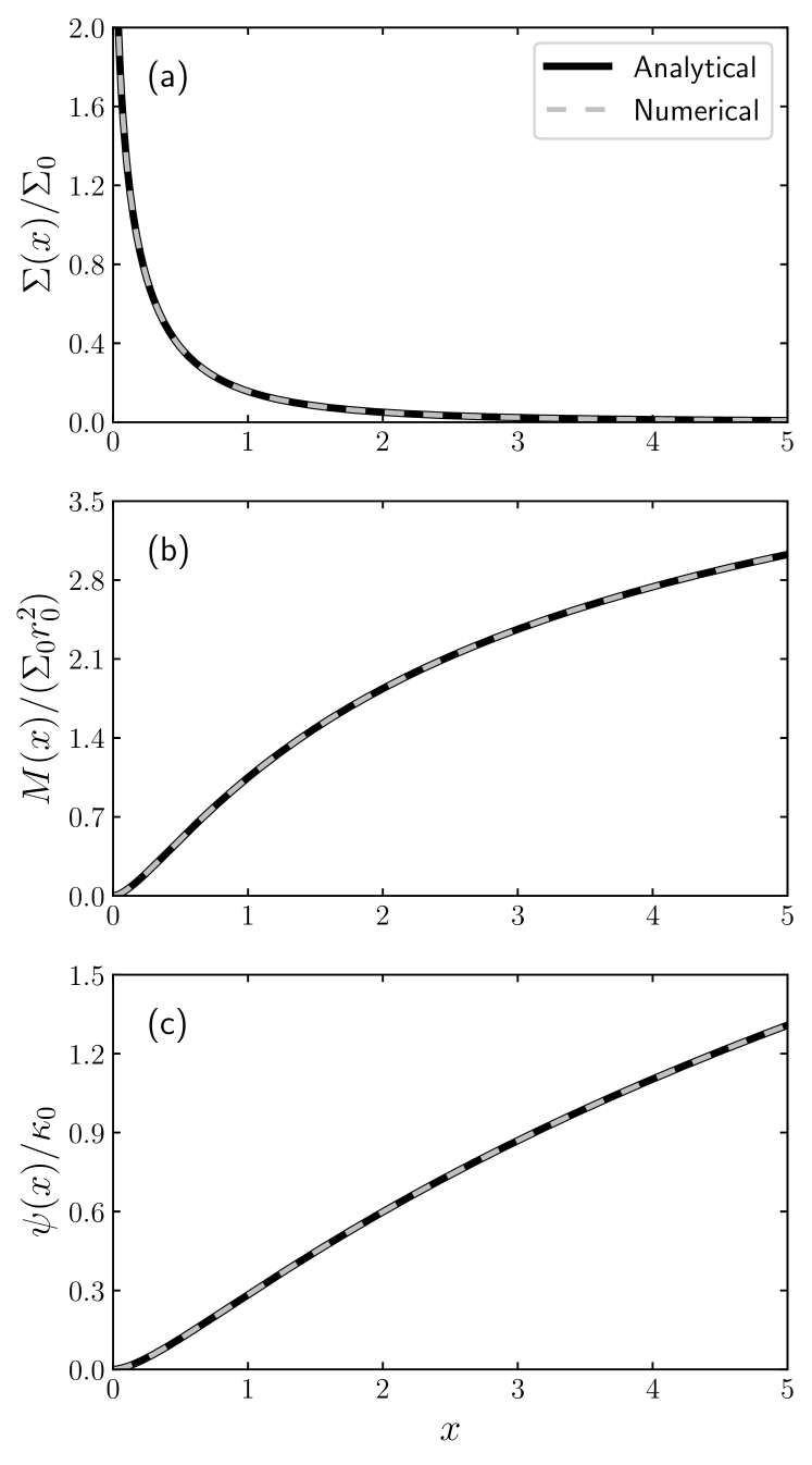
Figure 1: sNFW analytical (solid black curve) and numerical (dashed grey curve) normalised surface mass density (a), normalised projected mass (b), and normalised deflection potential (c).

In Fig. 1, we have the normalised surface mass density $\Sigma(x)/\Sigma_{0}$ (panel a), normalised projected mass $M(x)/(\Sigma_{0}r_{0}^{2})$ (panel b), and normalised deflection potential $\psi(x)/\kappa_{0}$ (panel c) given for the sNFW. There, the solid black curves represent the analytical expressions (69)-(71), while the dashed grey curves correspond to their numerical counterparts. Clearly, both analytical and numerical curves overlap, showing that expressions (69)-(71) are correct. Additionally, the normalised convergence turns out to be $\kappa(x)/\kappa_{0}=\Sigma(x)/\Sigma_{0}$. In Fig. 2 it is depicted the normalised deflection angle $\alpha(x)/\kappa_{0}$ (solid curve) and its derivative $\alpha^{\prime}(x)/\kappa_{0}$ (dashed curve), that are obtained from

$$\alpha(x)=\dfrac{2\kappa_{0}}{x}\begin{dcases}1-\dfrac{3\pi}{8\sqrt{2}}&\text{if }x=1\\ \dfrac{E\left(\frac{1-|x|}{1+|x|}\right)-|x|K\left(\frac{1-|x|}{1+|x|}\right)}{\sqrt{1+|x|}(|x|-1)}+1&\text{if }x\neq 1\end{dcases},$$ (74)

which is the result of substituting (70) into (5). In principle, (74) is discontinuous at $x=0$, however, this discontinuity is removable. This fact, along with how $\alpha^{\prime}(x)$ behaves, are important for the image formation process, which we discuss in the next section.

Lastly, in Fig. 3, we have the normalised shear $\gamma(x)/\kappa_{0}$ (dotted black curve) given by (5), and by (5) the mean shear (solid black curve) along with its numerical counterpart (dashed grey curve). Analytical and numerical curves coincide, indicating that (15) works correctly. At $x=0$, both shear and mean shear have the same value, as expected, which from (48) is $\gamma(0)/\kappa_{0}=\overline{\gamma}(0)/\kappa_{0}=3/8$. The signal is weakened when $x$ increases, in agreement with the loss in strength of the lens itself, as shown in Fig. 1 (panel a).

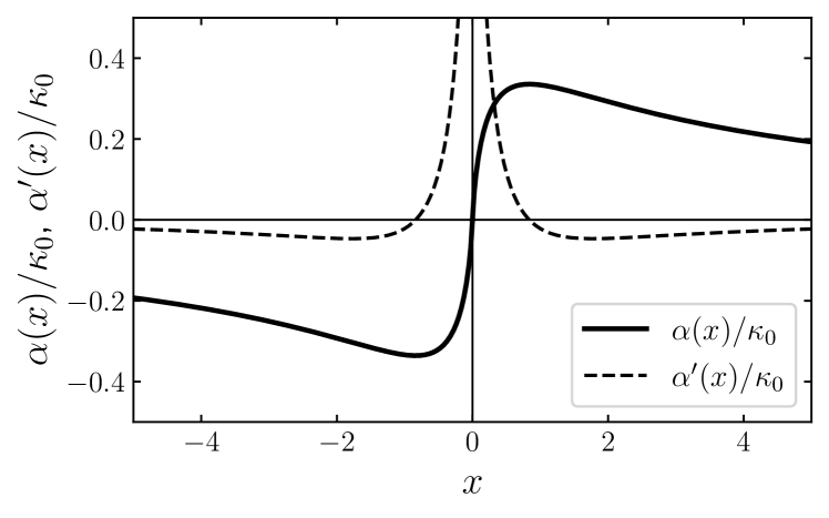
Figure 2: sNFW normalised deflection angle (solid curve) and its corresponding derivative (dashed curve).

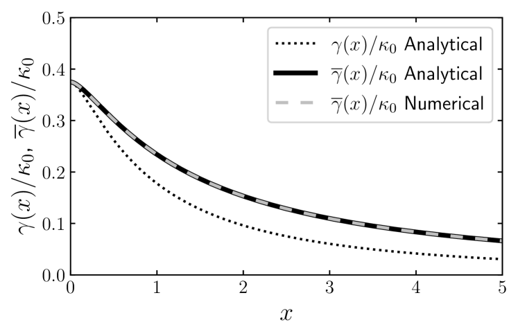
Figure 3: sNFW normalised shear $\gamma(x)/\kappa_{0}$ (dotted black curve), along with the analytical (solid black curve) and numerical (dashed grey curve) normalised mean shear $\overline{\gamma}(x)/\kappa_{0}$.

5.1 Image formation and magnification

Image formation depends strongly on the characteristic convergence $\kappa_{0}$. Fig. 4 depicts the lens equation given for $\kappa_{0}=1$ (solid curve), $\kappa_{0}=2$ (dashed curve) and, $\kappa_{0}=3$ (dotted curve). Since the deflection angle is proportional to $\kappa_{0}$, in all three cases the lens equation exhibits similar features. This holds true for any value of $\kappa_{0}$. In fact, the lens equation behaves like most asymmetric lenses, with the exception of, for example, the point-like lens and SIS.

All information regarding image formation is summarised in Fig. 5, where, for simplicity, we have restricted the radial coordinates to be non-negative. Hence, in the simpler scenario, consider a point-like source with position $\boldsymbol{y}=(y,\varphi)$ on the source plane, with $\varphi$ being its azimuthal coordinate. There, the black curve represents the lens equation, such that the solid part corresponds to the possible images on the lens plane with position $\boldsymbol{x}=(x,\varphi)$, whereas the dashed part corresponds to possible images with position $\boldsymbol{x}=(x,\varphi+\pi)$. The latter scenario provides the same information as Fig. 4 with $x<0$ and $y\geq 0$. The critical curves, at which the magnification $\mu(x)$ diverges, rule the presence of multiple images. The magnification is defined as

$$\dfrac{1}{\mu(x)}=(1-\kappa(x))^{2}-\gamma^{2}(x)=\dfrac{y(x)y^{\prime}(x)}{x},$$ (75)

which leads to two possible critical curves. The first one is the tangential critical curve, which is a circle, also known as Einstein’s ring, whose radius is $x_{\text{c1}}$ and satisfies $y(x)/x=1-\overline{\kappa}(x)=0$. The second one is the radial critical curve, which corresponds to a circle of radius $x_{\text{c2}}$ that satisfies $y^{\prime}(x)=1-\alpha^{\prime}(x)=1-2\kappa(x)+\overline{\kappa}(x)=0$. Note that $\overline{\kappa}(x)=\overline{\Sigma}(x)/\Sigma_{\text{cr}}=\alpha(x)/x$. Once the critical curves are mapped back into the source plane, we get the caustic curves. Those curves delimit the regions where a source will lead to multiple images. The tangential critical curve is mapped into $y_{\text{c1}}=0$, whereas the radial critical curve is mapped into a circle with radius $y_{\text{c2}}$. In Fig. 5 the position of critical curves and caustic curves are represented as vertical and horizontal black lines, respectively.

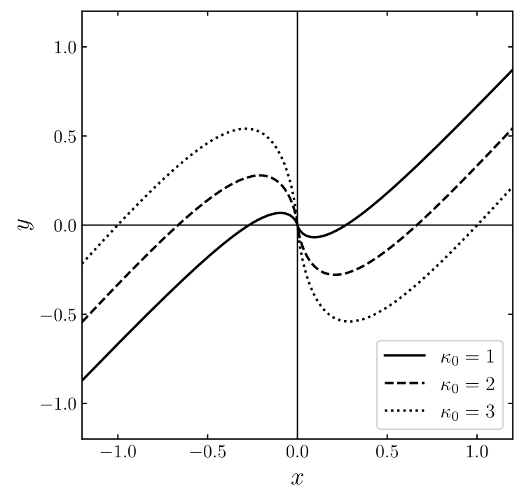
Figure 4: sNFW dimensionless lens equation (4) given for $\kappa_{0}=1$ (solid curve), $\kappa_{0}=2$ (dashed curve), and $\kappa_{0}=3$ (dotted curve).

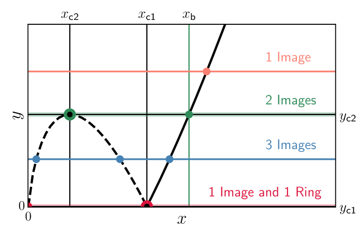
Figure 5: Image formation anatomy. The black curve represents the lens equation, such that for a source with position $\boldsymbol{y}=(y\geq 0,\varphi)$, it is possible to obtain images with position $\boldsymbol{x}=(x\geq 0,\varphi)$ (solid curve) or position $\boldsymbol{x}=(x\geq 0,\varphi+\pi)$ (dashed curve). The vertical and horizontal black lines represent the presence of critical and caustic curves, respectively. The additional horizontal lines show the possible scenarios of image formation depending on $y$, while the vertical green line at $x_{\text{b}}$ represents the boundary within which multiple images appear.

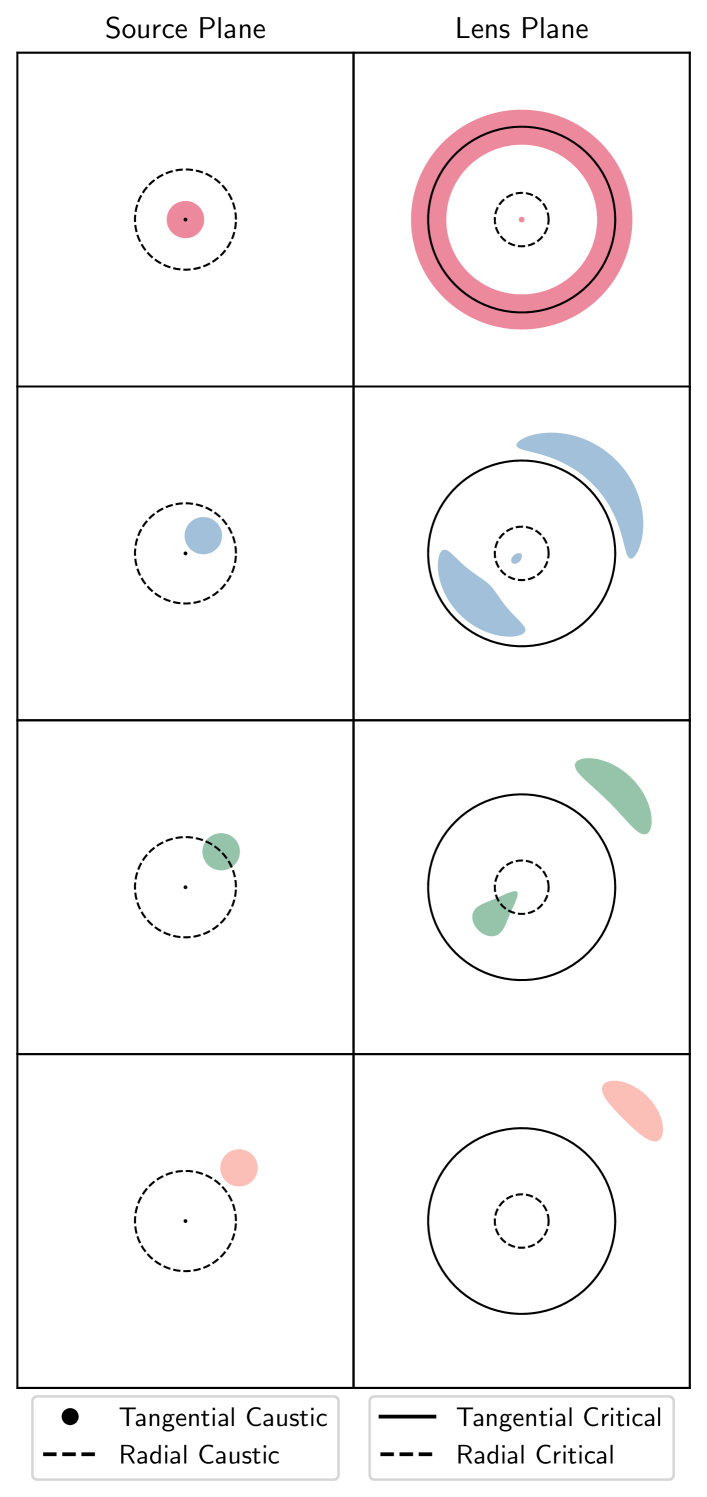
Figure 6: sNFW image formation example for an extended source with different positions relative to the caustic curves. Each colour matches one of the four scenarios described in Fig. 5.

From Fig. 5, we can see that for a source at $y=0$ (horizontal red line), we have two possible solutions to the lens equation. These solutions correspond to the critical curve $x_{\text{c1}}$ and one image at $x=0$. Such image does not correspond to a critical curve since, instead of having a divergent magnification, such image is demagnified. In other words, $\mu(x\to 0)=0$. Being a demagnified and faint image makes it difficult (if not impossible) to observe. For $0<y<y_{\text{c2}}$ (horizontal blue line), we get three images, where the two images with $0<x<c_{\text{c1}}$ have azimuthal coordinate $\varphi+\pi$. Those two images merge at $x_{\text{c2}}$ when the given source is located at $y_{\text{c2}}$, for which a second image is formed at $x>x_{\text{c1}}$ (horizontal green line). For $y>y_{\text{c2}}$ (horizontal orange line) only one image is formed at $x>x_{\text{c1}}$. These four possible scenarios are represented in Fig. 6 on the lens plane for an extended source with radius $0.2$ and a sNFW lens with $\kappa_{0}=3$.

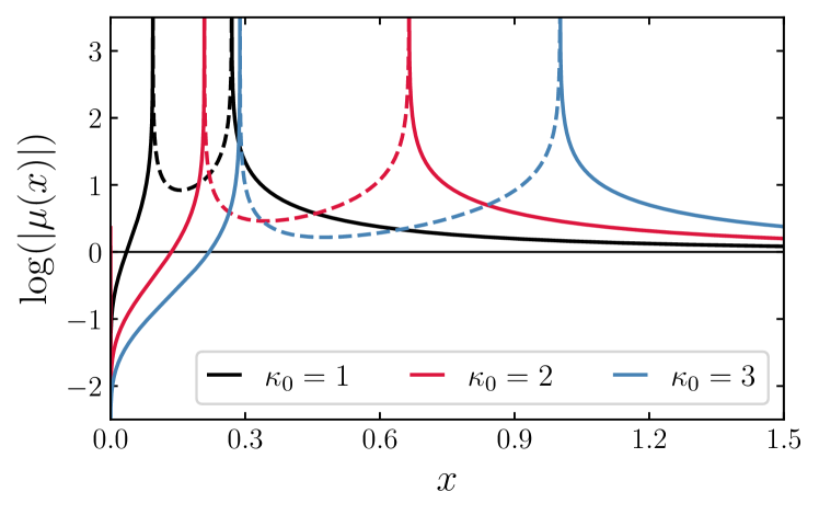
Figure 7: sNFW absolute magnification $\log(|\mu(x)|)$ curves given for $\kappa_{0}=1$ (black), $\kappa_{0}=2$ (blue), and $\kappa_{0}=3$ (red). The solid curves correspond to $\mu(x)>0$, while the dashed curves correspond to $\mu(x)<0$.

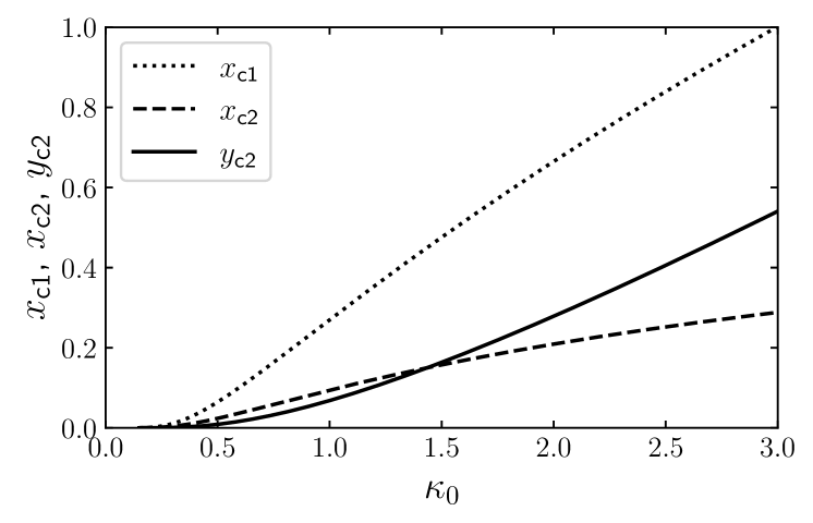
Figure 8: Tangential critical curve $x_{\text{c1}}$ (dotted), radial critical curve $x_{\text{c2}}$ (dashed), and the corresponding radial caustic curve $y_{\text{c2}}$ (solid). Provided that the tangential critical curve exists, irrespectively of $\kappa_{0}$ its corresponding caustic is $y_{\text{c1}}=0$.

Fig. 7 shows the absolute magnification $\log(|\mu(x)|)$ given for $\kappa_{0}=1$ (black curve), $\kappa_{0}=2$ (red curve), and $\kappa_{0}=3$ (blue curve). We see two vertical asymptotes, which represent the critical curves. The inner one is the radial critical curve, while the outer one is the tangential critical curve. In terms of the signed magnification $\mu(x)$, the solid curves correspond to $\mu(x)>0$, while the dashed curves represent $\mu(x)<0$. Therefore, images that lie on $x_{\text{c2}}<x<x_{\text{c1}}$ have negative parity, whereas images that lie on $0<x<x_{\text{c2}}$ and $x>x_{\text{c1}}$ have positive parity. As $\kappa_{0}$ increases, we can see in Fig. 8 that the critical curves move away from the centre, and the separation between critical curves increases, always with $x_{\text{c1}}>x_{\text{c2}}$, which is quite evident in Fig. 7. From Fig. 8, we can also see that $x_{\text{c2}}>y_{\text{c2}}$ for small values of $\kappa_{0}$, however, eventually (around $\kappa_{0}\sim 1.4$) this relation flips and we get $y_{\text{c2}}>x_{\text{c2}}$. For higher values of $\kappa_{0}$, the radial critical curve keeps increasing its size, but the radial caustic grows faster. This implies that when $\kappa_{0}$ increases it becomes easier to get multiple images, and since in terms of proportion the region within the radial critical curve is smaller, it is more likely to get a faint image closer to the lens centre.

Provided that sources are not located at caustics, we get either one or three images, consistent with the odd images theorem. First explored in spherical galaxies by Dyer & Roeder (1980) and then generalised by Burke (1981), it requires lenses to have a non-singular mass distribution. Nevertheless, it was shown by Bartelmann (1996) that a mass distribution such as the NFW, despite of being singular at its centre, it possesses a radial critical curve, forming an odd number of images. He argued that this is possible since $\alpha^{\prime}(x)$ is continuous (at least for $x>0$), and $\alpha^{\prime}(x\to 0)=\infty$ and $\alpha^{\prime}(x\to\infty)=0$. This basically guaranties that there exists a $x$ for which $\alpha^{\prime}(x)=1$. From Fig. 2 (dashed curve) it is straightforward to see that these conditions are also fulfilled by the sNFW. As well, as discussed in Mollerach & Roulet (2002), the appearance of an odd number of images can be argue from considering the deflection angle being bounded and continuous at $x=0$ . Alternatively, from the perspective of the deflection potential, theorem 1 in Petters & Werner (2010) indicates that the total number of images is given by $N=2N_{+}+g-1$, where $N_{+}$ is the number of images with positive parity, and $g$ is the number of infinite singularities of $\psi$, which are those $x_{s}$ for which $\psi(x\to x_{s})=-\infty$. In our case, since $g=0$, this theorem predicts $N=3$ for sources with $0<y<y_{\text{c2}}$, and $N=1$ for sources with $y>y_{\text{c2}}$. Ultimately, the condition of the mass distribution being non-singular is more a sufficient than a necessary condition for getting an odd number of images.

5.2 Magnification invariant

For a source inside the caustic that produces the maximum possible number of images, $I=\sum_{i}\mu_{i}$ represents the sum of their corresponding (signed) magnification. It has been shown that for certain lenses, $I$ is constant and independent of most of their parameters. Therefore, it is usually referred to as the magnification invariant. That is the case, for example, of a systems of n-point lenses (Witt & Mao, 1995; Rhie, 1997), and the Plummer lens (Werner & Evans, 2006), for which $j=1$. The magnification invariant has also been analytically computed for models intended to fit quadruple lenses, such as variations of the SIS model (Dalal, 1998; Witt & Mao, 2000; Dalal & Rabin, 2001; Hunter & Evans, 2001). More recently, Wei et al. (2018) have explored how $I$ behaves for axisymmetric lenses such as the NFW, Einasto (for $n=1/2,1$), an exponential disc and, the modified Hubble model.

In our case, we know that the sNFW produces at most three images, and this occurs when the source is inside the radial caustic but not on any caustic. Hence, given a source with $0<y<y_{\text{c2}}$, each of its images appears inside one of three possible regions, namely: region 1 ($0<x<x_{\text{c2}}$), region 2 ($x_{\text{c2}}<x<x_{\text{c1}}$),and region 3 ($x_{\text{c1}}<x<x_{\text{b}}$), where $x_{\text{b}}$ (depicted as the vertical green line in Fig. 5) represents the external limit within which multiple images are present.

In order to evaluate $I$, we need to solve the lens equation (4) accurately. To do so, for a source with position $y_{0}$, we divide region 1 in $N$ nodes and map all of them into the source plane by means of (4). Then, the node that is mapped closest to $y_{0}$ corresponds to the image $x_{1}$. We apply this process for regions 2 and 3 as well in order to find $x_{2}$ and $x_{3}$, respectively. This process can be done using an adaptive refinement on each region. This approach to solving (4) is computationally inexpensive and accurate, leading, on average, to relative errors of $\sim 10^{-10}$ or smaller. We test this approach, and our implementation by applying it to the Non-Singular Isothermal Sphere (NIS) given in Appendix C. Such NIS produces at most three images, for which Wei et al. (2018) showed analytically that $I_{\text{NIS}}=2$, independent of any parameter.

Figure 9: Given a $\kappa_{0}$, we evaluate $I_{\text{NIS}}$ for several sources inside the radial caustic. The corresponding average value $\braket{I_{\text{NIS}}}$ for such $\kappa_{0}$ is depicted as a data-point, where the error bars represent the standard deviation. Here, we plot $\braket{I_{\text{NIS}}}$ as a function of $\kappa_{0}$.

What we do here is, given a $\kappa_{0}$, for several sources within $0<y<y_{\text{c2}}$, we solve the lens equation and compute their corresponding $I_{\text{NIS}}$. Then, we take its average value $\braket{I_{\text{NIS}}}$, which is represented as a point in Fig. 9. Its standard deviation is represented as error bars. For any $\kappa_{0}$ we get $\braket{I_{\text{NIS}}}=2$, with a negligible standard deviation of about $10^{-12}$ or smaller (no error bars), as it can be seen in Fig. 9. Thus, this result shows that the approach being used works correctly.

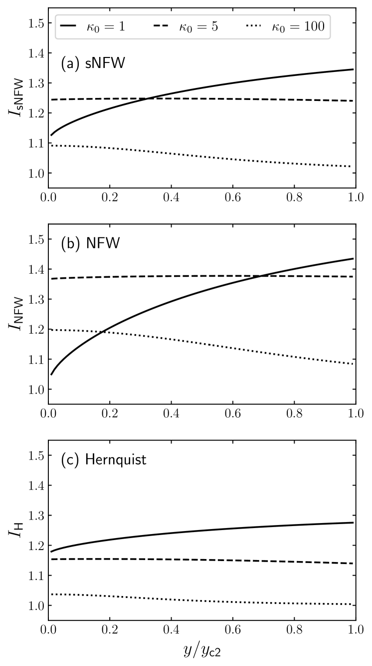
Figure 10: $I$ as function of $y/y_{\text{c2}}$ for $\kappa_{0}=1$ (solid), $\kappa_{0}=5$ (dashed) and, $\kappa_{0}=100$ (dotted). These curves are given for the sNFW (a), NFW (b), and Hernquist (c) lenses.

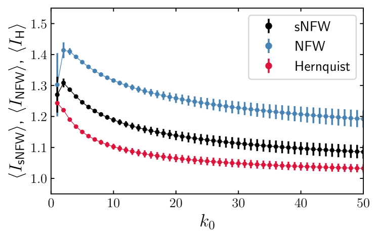
Figure 11: Same as in Fig. 9, but for the sNFW (black), NFW (blue), and Hernquist (red) lenses.

Considering $\kappa_{0}=1,5,100$, for the sNFW, we have computed $I_{\text{sNFW}}$ for several sources inside the respective radial caustic $0<y<y_{\text{c2}}$. They are depicted in Fig. 10 (panel a) as functions of $y/y_{\text{c2}}$. For $k_{0}=1$ (solid curve), it is evident that $I_{\text{sNFW}}$ is not constant, it actually varies within $1.27_{-0.14}^{+0.07}$. For $\kappa_{0}=5$ (dashed curve) it is approximately constant with $I_{\text{sNFW}}\approx 1.24$, and when $\kappa_{0}$ increases the deviations also increase, so that for $\kappa_{0}=100$ (dotted curve), we get $I_{\text{sNFW}}$ to be within $1.06_{-0.04}^{+0.03}$. This behaviour is not exclusive to the sNFW, since as we can see in Fig. 10 (panels b and c), the NFW and Hernquist lenses exhibit a similar behaviour. By applying the same procedure used to construct Fig. 9, we get Fig. 11, which shows $\braket{I}$ as a function of $\kappa_{0}$ for the sNFW (black), NFW (blue), and Hernquist (red) lenses. There, for those three lenses, we have that $\braket{I}$ decreases when $\kappa_{0}$ increases, which is consistent with the behaviour reported by Wei et al. (2018) for the NFW. We also have that higher variations in $I$ occur for $\kappa_{0}\lesssim 1$, while it can be considered to be (approximately) constant for $\kappa_{0}$ between $2$ and $10$. Depending on the observational uncertainties this range can be extended. Strictly speaking, we cannot say that for the sNFW, NFW, and Hernquist lenses $I$ is invariant once a $\kappa_{0}$ is given. However, the variations of $I$ as function of $y/y_{\text{c2}}$ are small enough, such that, when modelling astrophysical systems it can be used to validate or discard models, as it is discussed in e.g., Dalal (1998); Witt & Mao (2000).

6 Summary and conclusions

In this paper, we use the Fox $H$-function as a tool to describe analytically the gravitational lensing properties of the gNFW profile given by (1), focusing on the sNFW ($n=7/2$) (Lilley et al., 2018). To do so, we provide a description of how we can write the projected mass and deflection potential in terms of the Fox $H$-function, whenever we have a lens whose surface mass density satisfies (16). For the gNFW, using this procedure along with the Mellin technique explained in Appendix A, we give analytical expressions for its surface mass density (41), projected mass (42), and deflection potential (43) in terms of three independent Fox $H$-functions. From them, it is straightforward to compute its corresponding convergence, deflection angle, shear, and mean shear. We also provide the power (logarithmic) series representations for such Fox $H$-functions, following Kilbas & Saigo (1999); Kilbas (2004). A general description of the Fox $H$-function with the relevant aspects used in this paper can be found in Appendix B. It can be shown from such series representations that (41)-(43) converge to the well known analytical expressions for the NFW ($n=3$) and Hernquist ($n=4$) lenses, listed in Appendix D.

In the particular case of the sNFW, the required Fox $H$-functions converge to closed-form expressions in terms of the complete elliptic functions of first and second kind $K$ and $E$, respectively. Its surface mass density (69) is equivalent to the expression reported in Lilley et al. (2018), while its projected mass (70) and deflection potential (71) have not yet been reported in the literature, which are fundamental to describe this axisymmetric lens. We also provide explicit analytical expressions for its deflection angle (74), shear (5), and mean shear (5). The sNFW produces at most three images as long as the source is located inside the radial caustic. For such a scenario, we found that for a fixed $\kappa_{0}$, the sum of their signed magnification $I$ is not constant (strictly speaking), instead, $I$ depends on the position of the source inside the radial caustic. For $\kappa_{0}\lesssim 1$, we see that $I$ exhibits the largest variations, while in a good approximation $I$ can be considered as a constant when $\kappa_{0}$ is within the range $2-10$ (approximately). For higher values of $\kappa_{0}$, the variations on $I$ increase again, although they are within the observational uncertainties. This behaviour is shared with the NFW and Hernquist lenses. As a function of $\kappa_{0}$, for those three lenses we see that $I$ decreases when $\kappa_{0}$ increases, but not at a constant rate. This behaviour is consistent with the results reported by Wei et al. (2018) for the NFW. Among these three lenses, the Hernquist lens is the one that exhibits the smallest variations on $I$ for a given $\kappa_{0}$.

One natural next step in the understanding of the sNFW is to test how well the sNFW performs the task of modelling the dark matter component of astrophysical lenses, not only at galactic scales, but also in the context of galaxy groups and galaxy clusters. Moreover, the addition of an ellipticity or external shear should be explored. With this, it is interesting to see if $I$ maintains its behaviour after the appearance of cusps and folds for one of the caustics, along with the study of the magnification relations at cusps and folds. However, these ideas lie beyond the scope of this paper, and we leave them for future work.

Appendix A The Mellin transform technique

Given a function $f$, its Mellin transform is an integral transformation defined as

$$F(u)=\mathfrak{M}_{f}(u)=\int_{0}^{\infty}f(x)x^{u-1}dx,$$ (76)

where $u\in\mathbb{C}$. Likewise, the inverse transform of $F$ takes the form

$$f(x)=\mathfrak{M}^{-1}_{F}(x)=\dfrac{1}{2\pi i}\int_{\mathcal{L}}F(u)x^{-u}du,$$ (77)

with $\mathcal{L}$ being parallel to the imaginary axis in the complex plane.

Now, if $f$ can be written as the Mellin convolution of two functions, namely $f_{1}$ and $f_{2}$, which reads

$$f(x)=(f_{1}\star f_{2})(x)=\int_{0}^{\infty}t^{-1}f_{1}(t)f_{2}(x/t)dt,$$ (78)

its Mellin transform turns out to be

$$F(u) =\mathfrak{M}_{f_{1}\star f_{2}}(u)$$

$$=\int_{0}^{\infty}(f_{1}\star f_{2})(x)x^{u-1}dx$$

$$=\int_{0}^{\infty}f_{1}(t)\left(\int_{0}^{\infty}f_{2}(x/t)x^{u-1}t^{-1}dx\right)dt,$$ (79)

such that, if we consider $y=x/t$, it is easy to show that

$$F(u)=\mathfrak{M}_{f_{1}\star f_{2}}(u)=\mathfrak{M}_{f_{1}}(u)\mathfrak{M}_{f_{2}}(u).$$ (80)

Finally, by applying the inverse Mellin transform (77) to (80), it follows

$$f(x)=\mathfrak{M}^{-1}_{F}(x)=\dfrac{1}{2\pi i}\int_{\mathcal{L}}\mathfrak{M}_{f_{1}}(u)\mathfrak{M}_{f_{2}}(u)x^{-u}du,$$ (81)

which smoothly leads us to the definition of the Fox $H$-function when $\mathfrak{M}_{f_{1}}$ and $\mathfrak{M}_{f_{2}}$ are given as the product of Gamma functions, as we discuss in Appendix B.

Appendix B The Fox $H$-function

The Fox $H$-function was first introduced in Fox (1961) as the generalisation of the Meijer $G$-function.

Here, we provide the definition and properties of the Fox $H$-function needed to describe the gNFW halo as a gravitational lens. For a more extensive and exhaustive description of the Fox H-function, refer to e.g., Kilbas & Saigo (1999); Kilbas (2004). The Fox H-function is in general a complex valued function defined by the Mellin-Barnes integral

$$\displaystyle H_{p,q}^{m,n}(x) =H_{p,q}^{m,n}\!\left[x\left|\begin{matrix}(a_{1},A_{1}),\ldots,(a_{p},A_{p})\\ (b_{1},B_{1}),\ldots,(b_{q},B_{q})\end{matrix}\right.\right]$$

$$=\dfrac{1}{2\pi i}\int_{\mathcal{L}}\Theta(u)x^{-u}du$$ (82)

with

$$\Theta(u)=\dfrac{\displaystyle\prod_{j=1}^{m}\Gamma(b_{j}+B_{j}u)\prod_{j=1}^{n}\Gamma(1-a_{j}-A_{j}u)}{\displaystyle\prod_{j=n+1}^{p}\Gamma(a_{j}+A_{j}u)\prod_{j=m+1}^{q}\Gamma(1-b_{j}-B_{j}u)},$$ (83)

where $m,n,p,q\in\mathbb{N}_{0}$, $A_{j}\,(j=1,\ldots,p)$ and $B_{j}\,(j=1,\ldots,q)$ are positive real numbers, while $a_{j}\,(j=1,\ldots,p)$ and $b_{j}\,(j=1,\ldots,q)$ are complex numbers (in general). The contour $\mathcal{L}$ separates the poles of $\prod_{j=1}^{m}\Gamma(b_{j}+B_{j}u)$ from those of $\prod_{j=1}^{n}\Gamma(1-a_{j}-A_{j}u)$. When in (83), all $A_{j}=1$ ($j=1,\ldots,p$) and all $B_{j}=1$ ($j=1,\ldots,q$), the Fox $H$-function reduces to the Meijer $G$-function

$$\displaystyle G_{p,q}^{m,n}(x)=G_{p,q}^{m,n}\!\left[x\left|\begin{matrix}a_{1},\ldots,a_{p}\\ b_{1},\ldots,b_{q}\end{matrix}\right.\right].$$

Following Kilbas & Saigo (1999), in order to evaluate (B), we work with its corresponding power (logarithmic) series expansion. Such series representation depends on the multiplicity of the poles

$$\beta_{j}=-\left(\dfrac{b_{j}+k_{j}}{B_{j}}\right)\quad(j=1,\dots,m\quad\text{and}\quad k_{j}\in\mathbb{N}_{0})$$ (84)

and

$$\alpha_{j}=\dfrac{1-a_{j}+k_{j}}{A_{j}}\quad(j=1,\dots,n\quad\text{and}\quad k_{j}\in\mathbb{N}_{0}),.$$ (85)

corresponding to the gamma functions $\Gamma(b_{j}+B_{j}u)$ and $\Gamma(1-a_{j}-A_{j}u)$ in (83), respectively. For such series representation to converge it is required that either (see Theorems 2-6 in Kilbas & Saigo (1999))

• Case 1: $\Delta>0$ and $x\neq 0$ or $\Delta=0$ and $0<|x|<\delta$

• Case 2: $\Delta<0$ and $x\neq 0$ or $\Delta=0$ and $|x|>\delta$

with

$$\Delta=\sum_{j=1}^{q}B_{j}-\sum_{j=1}^{p}A_{j}\quad\text{and}\quad\delta=\prod_{j=1}^{q}B_{j}^{B_{j}}\prod_{j=1}^{p}A_{j}^{-A_{j}}.$$ (86)

Then, for both cases, (B) can be written as

$$H_{p,q}^{m,n}(x)=\underbrace{\sum_{i}\sum_{k_{i}}\mathcal{C}_{1i}x^{-u_{pi}}}_{\text{Simple poles}}$$

$$+\underbrace{\sum_{k_{1}}\mathcal{C}_{2}x^{-u_{p1}}\left(\mathcal{C}^{\prime}_{2}-\ln(x)\right)}_{\text{Second order poles}}$$

$$+\underbrace{\sum_{k_{1}}\mathcal{C}_{3}x^{-u_{p1}}\left(\dfrac{1}{2}\mathcal{C}^{\prime 2}_{3}+\dfrac{1}{2}\mathcal{C}^{\prime\prime}_{3}-\mathcal{C}^{\prime}_{3}\ln(x)+\dfrac{1}{2}\ln^{2}(x)\right)}_{\text{Third order poles}},$$ (87)

where we consider the series expansion for poles up to third order. In particular, we make explicit the possibility of having several gamma functions with simple poles, while for higher order poles we only consider the possibility of having one pair or triplet of functions with second or third order poles, respectively. This is what face in this work. In Kilbas & Saigo (1999) they provide the general expansion for poles of arbitrary order $N$, which reduces to the terms in (B) after some algebra.

The form taken by $\mathcal{C}_{l}$, $\mathcal{C}^{\prime}_{l}$, and $\mathcal{C}^{\prime\prime}_{l}$ (with $l=1,2,3$ as appropriate) in (B), depends on each of the aforementioned cases, which we make explicit below.

Case 1: In this case the poles of interest are those from the gamma functions $\Gamma(b_{i}+B_{i}u)$ $(i=1,\dots,m)$, with at most $m$ of them with simple poles of the form $u_{pi}=\beta_{i}$ (see (84)), for which

$$\mathcal{C}_{1i}=\dfrac{(-1)^{k_{i}}}{B_{i}k_{i}!}\dfrac{\displaystyle\prod_{\begin{subarray}{c}j=1\\ j\neq i\end{subarray}}^{m}\Gamma(b_{j}+B_{j}\beta_{i})\prod_{j=1}^{n}\Gamma(1-a_{j}-A_{j}\beta_{i})}{\displaystyle\prod_{j=n+1}^{p}\Gamma(a_{j}+A_{j}\beta_{i})\prod_{j=m+1}^{q}\Gamma(1-b_{j}-B_{j}\beta_{i})},$$ (88)

while for higher order poles we have $u_{p1}=\beta_{1}$ (see (84)), where $\beta_{1}=\beta_{2}$ for second order poles and $\beta_{1}=\beta_{2}=\beta_{3}$ for third order poles. These relations allow us to write $k_{2}$ and $k_{3}$ in terms of $k_{1}$, since for $l=2,3$

$$\mathcal{C}_{l}=\left(\prod_{j=1}^{l}\dfrac{(-1)^{k_{j}}}{B_{j}k_{j}!}\right)\dfrac{\displaystyle\prod_{j=l+1}^{m}\Gamma(b_{j}+B_{j}\beta_{1})\prod_{j=1}^{n}\Gamma(1-a_{j}-A_{j}\beta_{1})}{\displaystyle\prod_{j=n+1}^{p}\Gamma(a_{j}+A_{j}\beta_{1})\prod_{j=m+1}^{q}\Gamma(1-b_{j}-B_{j}\beta_{1})},$$ (89)

$$\mathcal{C}^{\prime}_{l} =\sum_{j=l+1}^{m}B_{j}\psi_{0}(b_{j}+B_{j}\beta_{1})-\sum_{j=1}^{n}A_{j}\psi_{0}(1-a_{j}-A_{j}\beta_{1})$$

$$-\sum_{j=n+1}^{p}A_{j}\psi_{0}(a_{j}+A_{j}\beta_{1})+\sum_{j=m+1}^{q}B_{j}\psi_{0}(1-b_{j}-B_{j}\beta_{1})$$

$$+\sum_{j=1}^{l}B_{j}\psi_{0}(1+k_{j})$$ (90)

and,

$$\mathcal{C}^{\prime\prime}_{3} =\sum_{j=4}^{m}B_{j}^{2}\psi_{1}(b_{j}+B_{j}\beta_{1})+\sum_{j=1}^{n}A_{j}^{2}\psi_{1}(1-a_{j}-A_{j}\beta_{1})$$

$$-\sum_{j=n+1}^{p}A_{j}^{2}\psi_{1}(a_{j}+A_{j}\beta_{1})-\sum_{j=m+1}^{q}B_{j}^{2}\psi_{1}(1-b_{j}-B_{j}\beta_{1})$$

$$+\sum_{j=1}^{3}B_{j}^{2}\left(\dfrac{\pi^{2}}{3}-\psi_{1}(1+k_{j})\right).$$ (91)

Case 2: In this case the poles of interest are those from the gamma functions $\Gamma(1-a_{i}-A_{i}u)$ $(i=1,\dots,n)$, with at most $n$ of them with simple poles of the form $u_{pi}=\alpha_{i}$ (see (85)), for which

$$\mathcal{C}_{1i}=\dfrac{(-1)^{k_{i}}}{A_{i}k_{i}!}\dfrac{\displaystyle\prod_{j=1}^{m}\Gamma(b_{j}+B_{j}\alpha_{i})\prod_{\begin{subarray}{c}j=1\\ j\neq i\end{subarray}}^{n}\Gamma(1-a_{j}-A_{j}\alpha_{i})}{\displaystyle\prod_{j=n+1}^{p}\Gamma(a_{j}+A_{j}\alpha_{i})\prod_{j=m+1}^{q}\Gamma(1-b_{j}-B_{j}\alpha_{i})},$$ (92)

while for higher order poles we have $u_{p1}=\alpha_{1}$ (see (85)), where $\alpha_{1}=\alpha_{2}$ for second order poles and $\alpha_{1}=\alpha_{2}=\alpha_{3}$ for third order poles. These relations allow us to write $k_{2}$ and $k_{3}$ in terms of $k_{1}$, which we need since for $l=2,3$

$$\mathcal{C}_{l}=-\left(\prod_{j=1}^{l}\dfrac{(-1)^{k_{j}-1}}{A_{j}k_{j}!}\right)\dfrac{\displaystyle\prod_{j=1}^{m}\Gamma(b_{j}+B_{j}\alpha_{1})\prod_{i=l+1}^{n}\Gamma(1-a_{j}-A_{j}\alpha_{1})}{\displaystyle\prod_{j=n+1}^{p}\Gamma(a_{j}+A_{j}\alpha_{1})\prod_{j=m+1}^{q}\Gamma(1-b_{j}-B_{j}\alpha_{1})},$$ (93)

$$\mathcal{C}^{\prime}_{l} =\sum_{j=1}^{m}B_{j}\psi_{0}(b_{j}+B_{j}\alpha_{1})-\sum_{j=l+1}^{n}A_{j}\psi_{0}(1-a_{j}-A_{j}\alpha_{1})$$

$$-\sum_{j=n+1}^{p}A_{j}\psi_{0}(a_{j}+A_{j}\alpha_{1})+\sum_{j=m+1}^{q}B_{j}\psi_{0}(1-b_{j}-B_{j}\alpha_{1})$$

$$-\sum_{j=1}^{l}A_{j}\psi_{0}(1+k_{j})$$ (94)

and,

$$\mathcal{C}^{\prime\prime}_{3} =\sum_{j=1}^{m}B_{j}^{2}\psi_{1}(b_{j}+B_{j}\alpha_{1})+\sum_{j=4}^{n}A_{j}^{2}\psi_{1}(1-a_{j}-A_{j}\alpha_{1})$$

$$-\sum_{j=n+1}^{p}A_{j}^{2}\psi_{1}(a_{j}+A_{j}\alpha_{1})-\sum_{j=m+1}^{q}B_{j}^{2}\psi_{1}(1-b_{j}-B_{j}\alpha_{1})$$

$$+\sum_{j=1}^{3}A_{j}^{2}\left(\dfrac{\pi^{2}}{3}-\psi_{1}(1+k_{j})\right).$$ (95)

As a final remark, when working with (B) it s useful to keep in mind that

$$\lim_{x\to-k}\dfrac{1}{\Gamma(1+x)}=\dfrac{1}{\Gamma(1-k)}=0,$$ (96)

$$\lim_{x\to-k}\dfrac{\psi_{0}(1+x)}{\Gamma(1+x)}=\dfrac{\psi_{0}(1-k)}{\Gamma(1-k)}=(-1)^{k}\Gamma(k),$$ (97)

$$\lim_{x\to-k}\dfrac{\psi_{1}(1+x)}{\Gamma(1+x)^{2}}=\dfrac{\psi_{1}(1-k)}{\Gamma(1-k)^{2}}=\Gamma(k)^{2},$$ (98)

with $k\in\mathbb{Z}^{+}$.

Appendix C A simple application case

Consider a Singular Isothermal Sphere (SIS) whose mass density is given by

$$\rho_{\text{SIS}}(r)=\dfrac{\sigma_{v}^{2}}{2\pi Gr^{2}}$$ (99)

where $\sigma_{v}$ is the velocity dispersion, and $G$ is the gravitational constant. Its corresponding surface mass density, given in terms of the Abel integral (30) (in analogy to (31)) reads

$$\Sigma_{\text{SIS}}(x)=\dfrac{\sigma^{2}_{v}}{\pi G\xi_{0}}\int_{x}^{\infty}\dfrac{db}{b\sqrt{b^{2}-x^{2}}},$$ (100)

with $b=r/\xi_{0}$, where in this case the normalisation scale length $\xi_{0}$ could be, for example, the Einstein’s radius. When we write (100) as the Mellin convolution (78) between $f_{1,\text{SIS}}$ and $f_{2,\text{SIS}}$, we have that

$$f_{1,\text{SIS}}(t=b)=\dfrac{\sigma^{2}_{v}}{\pi G\xi_{0}},$$ (101)

for which its Mellin transform $\mathfrak{M}_{f_{1},\text{SIS}}$ (see (76)) does not converge. This result is enough to conclude that (100) cannot be written as (81), and, in consequence, it cannot be given in terms of the Fox $H$-Function. At least, not by this means.

If we add a core with radius $r_{c}$ by means of $r^{2}\to r^{2}+r^{2}_{c}$, we get a Non-Singular Isothermal Sphere (NIS) whose mass density is

$$\rho_{\text{NIS}}(r)=\dfrac{\sigma_{v}^{2}}{2\pi G\left(r^{2}+r_{c}^{2}\right)}.$$ (102)

This mass distribution is simple enough to describe as a gravitational lens by direct integration, as shown in Hinshaw & Krauss (1987). For this reason, it is a good exercise to describe it in terms of the Fox $H$-function. In particular, doing this exercise helps to become familiar to work with the series expansion (B).

Following the same process that we applied for the gNFW in Sec. 4, and by taking the normalisation scale length to be $\xi_{0}=r_{c}$, it can be shown without much trouble that for our NIS, its surface mass density can be written as the Mellin convolution (see (78)) between

$$f_{1,\text{NIS}}(t=b)=\dfrac{\sigma^{2}_{v}}{\pi Gr_{c}}\dfrac{t^{2}}{t^{2}+1}$$ (103)

and $f_{2,\text{NIS}}$, which turns out to be identical to (33). Their corresponding Mellin transforms (see (76)) are

$$\mathfrak{M}_{f_{1},\,\text{NIS}}(u)=-\dfrac{\sigma^{2}_{v}}{2\pi Gr_{c}}\Gamma\left(1-\frac{u}{2}\right)\left(\frac{u}{2}\right)$$ (104)

and (35), respectively. Therore, from (81) and using the change of variable $v=1+u/2$ (for convenience), the surface mass density becomes

$$\Sigma_{\text{NIS}}(x)=\Sigma_{0}^{\text{NIS}}x\left(\dfrac{1}{2\pi i}\int_{\mathcal{L}}\Theta_{\Sigma}^{\text{NIS}}(v)x^{-2v}dv\right),$$ (105)

with

$$\Theta_{\Sigma}^{\text{NIS}}(v)=\Gamma\left(-\frac{1}{2}+v\right)\Gamma(1-v)$$ (106)

and

$$\Sigma_{0}^{\text{NIS}}=\dfrac{\sigma_{v}^{2}}{2\sqrt{\pi}Gr_{c}},$$ (107)

where it is clear that (105) satisfies (16) with $a=1$ and $b=2$. Thus, from (106) along with the outline given in Sec. 3, we can write the surface mass density, projected mass, and deflection potential of our NIS explicitly in terms of the Fox $H$-function (B) as

$$\Sigma_{\text{NIS}}(x)=\Sigma_{0}^{\text{NIS}}xH_{1,1}^{1,1}\!\left[x^{2}\left|\begin{matrix}(0,1)\\ (-\frac{1}{2},1)\end{matrix}\right.\right],$$ (108)

$$M_{\text{NIS}}(x)=\pi r_{c}^{2}\Sigma_{0}^{\text{NIS}}x^{3}H^{1,2}_{2,2}\!\left[x^{2}\left|\begin{matrix}(0,1),(-\frac{1}{2},1)\\ (-\frac{1}{2},1),(-\frac{3}{2},1)\end{matrix}\right.\right],$$ (109)

$$\psi_{\text{NIS}}(x)=\dfrac{\kappa_{0}^{\text{NIS}}x^{3}}{2}H^{1,3}_{3,3}\!\left[x^{2}\left|\begin{matrix}(0,1),(-\frac{1}{2},1),(-\frac{1}{2},1)\\ (-\frac{1}{2},1),(-\frac{3}{2},1),(-\frac{3}{2},1)\end{matrix}\right.\right],$$ (110)

respectively.

From condition (86), we can show that the three Fox $H$-functions in (108)-(110) satisfy $\Delta=0$ and $\delta=1$. Hence, as described in B, they converge for $0<x^{2}<1$ and $x^{2}>1$. Thus, since for us $x$ is non-negative, (108)-(110) can be given as

$$\Sigma_{\text{NIS}}(x)=\Sigma_{0}^{\text{NIS}}\begin{dcases}\displaystyle\sum_{k=0}^{\infty}\dfrac{(-1)^{k}}{k!}\Gamma\left(\frac{1}{2}+k\right)x^{2k}&\text{if }0<x<1\\ \displaystyle\sum_{l=0}^{\infty}\dfrac{(-1)^{l}}{l!}\Gamma\left(\frac{1}{2}+l\right)x^{-2l-1}&\text{if }x>1\end{dcases}.$$ (111)

$$M_{\text{NIS}}(x)=\pi r_{c}^{2}\Sigma_{0}^{\text{NIS}}$$

$$\times\begin{dcases}\displaystyle\sum_{k=0}^{\infty}\dfrac{(-1)^{k}}{(1+k)!}\Gamma\left(\frac{1}{2}+k\right)x^{2k+2}&\text{if }0<x<1\\ \displaystyle 2\sum_{l=0}^{\infty}\dfrac{(-1)^{l}}{l!}\Gamma\left(\frac{1}{2}+l\right)\frac{x^{-2l+1}}{(1-2l)}-2\sqrt{\pi}&\text{if }x>1\end{dcases},$$ (112)

$$\psi_{\text{NIS}}(x)=\frac{\kappa_{0}^{\text{NIS}}}{2}$$

$$\times\begin{dcases}\displaystyle\sum_{k=0}^{\infty}\dfrac{(-1)^{k}}{k!}\Gamma\left(\frac{1}{2}+k\right)\frac{x^{2k+2}}{(1+k)^{2}}\qquad\qquad\qquad\text{if }0<x<1\\[15.0694pt] \displaystyle 4\sum_{l=0}^{\infty}\dfrac{(-1)^{l}}{l!}\Gamma\left(\frac{1}{2}+l\right)\frac{x^{-2l+1}}{(1-2l)^{2}}-4\sqrt{\pi}\left(\ln\left(\dfrac{x}{2}\right)+1\right)&\\ \qquad\qquad\qquad\qquad\qquad\qquad\qquad\qquad\qquad\quad\text{if }x>1\end{dcases}.$$ (113)

The discontinuities at $x=0$ and $x=1$ in (111)-(C) are removable, so that for $x\geq 0$ it can be shown that they converge to

$$\Sigma_{\text{NIS}}(x)=\dfrac{\sqrt{\pi}\Sigma_{0}^{\text{NIS}}}{\sqrt{1+x^{2}}},$$ (114)

$$M_{\text{NIS}}(x)=2\pi^{3/2}r_{c}^{2}\Sigma_{0}^{\text{NIS}}\left(\sqrt{1+x^{2}}-1\right),$$ (115)

$$\psi_{\text{NIS}}(x)=2\sqrt{\pi}\kappa_{0}^{\text{NIS}}\left(\sqrt{1+x^{2}}-\ln\left(\frac{1+\sqrt{1+x^{2}}}{2}\right)-1\right),$$ (116)

respectively. For this application case, it is worth noting that in all cases the Fox $H$-function coincides with the Meijer $G$-function.

Appendix D NFW and Hernquist

In this appendix, for the NFW and Hernquist profiles we list their analytical properties as gravitational lenses (see e.g, Bartelmann (1996); Keeton (2001)). For that task we use the auxiliary functions

$$f(x)=\begin{dcases}\operatorname{arccosh}{\left(\frac{1}{x}\right)}&\text{if }0<x<1\\ \arccos{\left(\frac{1}{x}\right)}&\text{if }x>1\end{dcases},$$ (117)

and

$$s(x)=\begin{dcases}1&\text{if }0<x<1\\ -1&\text{if }x>1\end{dcases},$$ (118)

to get more compact expressions. It can be shown that with the appropriate value for $n$, (41)-(43) along with (8) and (15) reduce to the expressions below. Keep in mind that they are valid for $x>0$, and the characteristic surface mass density for each lens are

$$\Sigma_{0}^{\text{NFW}}=2\sqrt{\pi}\rho_{c}r_{0}\quad\text{and}\quad\Sigma_{0}^{\text{H}}=\dfrac{M}{2\sqrt{\pi}r_{0}^{2}},$$ (119)

where for the NFW $\rho_{c}$ is a characteristic density, and for the Hernquist $M$ is its total mass. For both lenses $r_{0}$ is a scale length.

D.1 NFW

$$\Sigma_{\text{NFW}}(x)=\dfrac{\Sigma_{0}^{\text{NFW}}}{\sqrt{\pi}}\begin{dcases}\dfrac{1}{3}&\text{if }x=1\\ \dfrac{1}{x^{2}-1}\left(1-\frac{f(x)}{\sqrt{|1-x^{2}|}}\right)&\text{if }x\neq 1\end{dcases},$$ (120)

$$M_{\text{NFW}}(x)=2\sqrt{\pi}r_{0}^{2}\Sigma_{0}^{\text{NFW}}\begin{dcases}1-\ln(2)&\text{if }x=1\\ \ln\left(\dfrac{x}{2}\right)+\frac{f(x)}{\sqrt{|1-x^{2}|}}&\text{if }x\neq 1\end{dcases},$$ (121)

$$\psi_{\text{NFW}}(x)=\dfrac{\kappa_{0}^{\text{NFW}}}{\sqrt{\pi}}\begin{dcases}\ln^{2}\left(2\right)&\text{if }x=1\\ \ln^{2}\left(\dfrac{x}{2}\right)-s(x)f^{2}(x)&\text{if }x\neq 1\end{dcases},$$ (122)

$$\gamma_{\text{NFW}}(x)=\kappa_{0}^{\text{NFW}}/(\sqrt{\pi}x^{2})$$

$$\times\begin{dcases}\dfrac{5}{3}-2\ln\left(2\right)&\text{if }x=1\\ 2\ln\left(\dfrac{x}{2}\right)+\dfrac{x^{2}}{1-x^{2}}+\dfrac{(2-3x^{2})s(x)f(x)}{(|1-x^{2}|)^{3/2}}&\text{if }x\neq 1\end{dcases},$$ (123)

$$\overline{\gamma}_{\text{NFW}}(x)=2\kappa_{0}^{\text{NFW}}/(\sqrt{\pi}x^{2})$$

$$\times\begin{dcases}\ln^{2}\left(2\right)+\ln\left(2\right)-1&\text{if }x=1\\ \ln^{2}\left(\dfrac{x}{2}\right)-\ln\left(\dfrac{x}{2}\right)-s(x)f^{2}(x)-\dfrac{f(x)}{\sqrt{|1-x^{2}|}}&\text{if }x\neq 1\end{dcases}.$$ (124)

D.2 Hernquist

$$\Sigma_{\text{H}}(x)=\dfrac{\Sigma_{0}^{\text{H}}}{\sqrt{\pi}}\begin{dcases}\dfrac{4}{15}&\text{if }x=1\\ \dfrac{1}{(x^{2}-1)^{2}}\left(\frac{(2+x^{2})f(x)}{\sqrt{|1-x^{2}|}}-3\right)&\text{if }x\neq 1\end{dcases},$$ (125)

$$M_{\text{H}}(x)=2\sqrt{\pi}r_{0}^{2}\Sigma_{0}^{\text{H}}\begin{dcases}\dfrac{1}{3}&\text{if }x=1\\ \dfrac{x^{2}}{x^{2}-1}\left(1-\frac{f(x)}{\sqrt{|1-x^{2}|}}\right)&\text{if }x\neq 1\end{dcases},$$ (126)

$$\psi_{\text{H}}(x)=\dfrac{2\kappa_{0}^{\text{H}}}{\sqrt{\pi}}\begin{dcases}1-\ln\left(2\right)&\text{if }x=1\\ \ln\left(\dfrac{x}{2}\right)+\dfrac{f(x)}{\sqrt{|1-x^{2}|}}&\text{if }x\neq 1\end{dcases},$$ (127)

$$\gamma_{\text{H}}(x)=\dfrac{\kappa_{0}^{\text{H}}}{\sqrt{\pi}}\begin{dcases}\dfrac{2}{5}&\text{if }x=1\\ \dfrac{1+2x^{2}}{(x^{2}-1)^{2}}-\dfrac{3x^{2}f(x)}{(|1-x^{2}|)^{5/2}}&\text{if }x\neq 1\end{dcases},$$ (128)

$$\overline{\gamma}_{\text{H}}(x)=2\kappa_{0}^{\text{H}}/(\sqrt{\pi}x^{2})$$

$$\times\begin{dcases}\dfrac{5}{3}-2\ln\left(2\right)&\text{if }x=1\\ 2\ln\left(\dfrac{x}{2}\right)+\dfrac{x^{2}}{1-x^{2}}+\dfrac{(2-3x^{2})s(x)f(x)}{(|1-x^{2}|)^{3/2}}&\text{if }x\neq 1\end{dcases}.$$ (129)