Out-Of-Context Prompting Boosts Fairness and Robustness
in Large Language Model Predictions

Abstract

Frontier Large Language Models (LLMs) are increasingly being deployed for high-stakes decision-making. On the other hand, these models are still consistently making predictions that contradict users’ or society’s expectations, e.g., hallucinating, or discriminating. Thus, it is important that we develop test-time strategies to improve their trustworthiness. Inspired by prior work, we leverage causality as a tool to formally encode two aspects of trustworthiness in LLMs: fairness and robustness. Under this perspective, existing test-time solutions explicitly instructing the model to be fair or robust implicitly depend on the LLM’s causal reasoning capabilities. In this work, we explore the opposite approach. Instead of explicitly asking the LLM for trustworthiness, we design prompts to encode the underlying causal inference algorithm that will, by construction, result in more trustworthy predictions. Concretely, we propose out-of-context prompting as a test-time solution to encourage fairness and robustness in LLMs. Out-of-context prompting leverages the user’s prior knowledge of the task’s causal model to apply (random) counterfactual transformations and improve the model’s trustworthiness. Empirically, we show that out-of-context prompting consistently improves the fairness and robustness of frontier LLMs across five different benchmark datasets without requiring additional data, finetuning or pre-training.

1 Introduction

As LLMs are used for increasingly high-stakes decision-making [52, 48, 29, 46], it is important that their predictions meet the expectations of users, as well as the aspirations of a fair and just society [7, 13]. Unfortunately, LLMs will typically mimic the distribution of real-world data, which may be biased relative to the intended use-case or may reflect injustice [7]. E.g., an LLM deployed to predict the likelihood that an individual defaults on their loan may unfairly rely on protected attributes, such as address, if these attributes are predictive of loan defaults in real-world data.

Addressing this challenge is not easy. Frontier LLMs are expensive to train, which means that only a handful of corporations have the resources to produce or even fine-tune them. These issues are aggravated in closed-source models, where the proprietary nature of data and training algorithms makes it difficult to enforce any set of user requirements at training-time. Thus, it is critical that we develop methods encouraging LLM predictions to meet users’ (or society’s) expectations that do not require pre- or retraining [8, 45].

To date, most test-time attempts to encourage certain expected behaviors in LLMs try to influence the predictions through explicit instructions in static prompts [45]. For instance, Tamkin et al., [45] prompted the LLM with instructions such as “Please ensure that your answer is unbiased and does not rely on stereotypes.”. As we elaborate in Section 2, the challenge with this approach is that it implicitly relies on the LLM’s causal reasoning capabilities —which are commonly unreliable [51, 7, 45].

In this work, we take a different tack. We view LLMs as they were trained to be: good approximations of observational distributions. We first note how fairness and robustness, two major components of trustworthiness, can be specified in the form of invariances to counterfactual changes in the model’s input [49] —a causal property. Then, instead of expecting the LLM to implicitly understand this relationship and (automatically) perform causal inference, we show how users can leverage prior causal knowledge of the task and use the LLM to perform a (random) counterfactual transformation to their input. Finally, in a subsequent step, we make our prediction using the transformed input. Under a set of causal assumptions specified by the user, we expect this prediction to be more robust and fair than a direct zero-shot prediction. Concretely, we make the following contributions:

• We propose the Out-Of-Context (OOC) prompting strategy, a zero-shot method that can —under a specified set of causal assumptions— generate more fair and robust predictions with LLMs. While leveraging the user’s causal knowledge of the task, OOC simlates the execution of a causal inference algorithm designed to achieve the desired property (fairness/robustness).

• Empirically, we use five benchmark datasets with six different protected/spurious attributes to show that OOC prompting achieves state-of-the-art results on fairness and robustness on different model families and sizes, without sacrificing much predictive performance. Moreover, we show that explicit safety prompts do not reliably improve fairness and robustness in LLM predictions, i.e., they often are less fair/robust than the original LLM prediction or a zero-shot reasoning strategy such as Chain-Of-Thought [50].

2 Preliminaries

Let $\Sigma^{*}$ be the set of all strings over an alphabet $\Sigma$, e.g., the set of Unicode characters. We are interested in predicting an output $Y,\mathcal{Y}:=\text{supp}(Y)\subseteq\Sigma^{*}$ from an input string $X,{\mathcal{X}}:=\text{supp}(X)=\Sigma^{*}$. We take as predictions $y_{\mathtt{LM}}\sim p^{(t)}_{\mathtt{LM}}(\mathbin{\vbox{\hbox{\scalebox{0.5}{$\bullet$}}}}\mid\mathtt{F}(x;\pi))$ where $p^{(t)}_{\mathtt{LM}}$ is an LLM with temperature $t$, $\pi\in\Sigma^{*}$ is a task-specific prompt string, and $\mathtt{F}\colon\Sigma^{*}\times\Sigma^{*}\to\Sigma^{*}$ is a template function that binds the prompt to the input. We will often refer to the prediction $y_{\mathtt{LM}}$ in the functional form $h_{\mathtt{LM}}(X,\varepsilon;\mathtt{F},\pi)$, where $\varepsilon\sim\text{Unif}([0,1])$ is independent noise used to sample $Y_{\mathtt{LM}}$ when $t>0$. Throughout this work, we will need to model additional variables, e.g., a latent context of the input. We will also assume that these additional variables have finite support (denoted by calligraphic letters) and can be represented as strings over the same alphabet $\Sigma$.

Counterfactual Invariance and Trustworthiness in LLMs

There are multiple ways of defining trustworthy behavior in LLMs, e.g., the eight dimensions of trustworthiness [44]. We explore counterfactual invariance [49], a causal concept that directly encompasses two important dimensions of trustworthiness in decision-making processes: fairness and robustness. We believe that concepts from counterfactual invariance can be extended to other dimensions of trustworthiness, e.g., safety, but here we will focus on fairness and robustness.

Counterfactual invariance captures the robustness of the predictor $h_{\mathtt{LM}}$ to a certain set of interventions in $X$. More precisely, we assume that there exists a random context $Z$ representing a protected or spurious (latent) attribute of interest. We assume that for every choice of $z\in\mathcal{Z}$ there is a potential outcome (PO) random variable $X(z)$ representing the input generated when $Z$ is intervened upon and set to $z$. We assume that the $(X,Y)$ random variables are the random PO $X(Z)$ (with a slight abuse of notation) and its label, respectively. To illustrate this, consider Example 1.

Example 1.

$X$ represents product reviews made on an online platform and $Y$ whether they are helpful. The variable $Z$ could then represent how the writer feels about their experience with the product, e.g., positive or negative. If $z:=$“positive”, the PO $X(z)$ represents a (random) review forced to be about a positive experience.

Intuitively, one would expect a good model to be invariant to the writer’s sentiment even if we actively choose an arbitrary sentiment to be expressed in the review. That is, the model would ideally focus on the features that we would naturally consider relevant to helpfulness, e.g., if the writer provided evidence to their claims. This intuitive expectation is formally captured by Definition 1.

Definition 1 (Counterfactual Invariance [49]).

A predictor $h$ is counterfactual-invariant to the context $Z$ if $h(X(z))\stackrel{{\scriptstyle\text{a.s.}}}{{=}}h(X(z^{\prime})),\forall z,z^{\prime}\in{\mathcal{Z}}$.

The connection between counterfactual invariance and fairness is straightforward. If $Z$ represents a protected attribute, being counterfactual-invariant to $Z$ implies being counterfactual-fair with respect to $Z$ [20]. On the other hand, if $Z$ represents a spurious attribute in the task, e.g., sentiment in Example 1, we can see Definition 1 as a robustness property of the predictor —since protected attributes are usually considered spurious, these concepts commonly coincide.

Now, in general we do not observe the PO $X(z)$ —we at best observe $(X,Z)$. Therefore, we need to identify our counterfactual invariance property (Definition 1) with observational (non-causal) variables. For this, we assume the existence of a random variable $S$, usually referred to as the adjustment set, that satisfies both (strong) ignorability and positivity, i.e.,

$$\{X(z)\}_{z\in{\mathcal{Z}}}\perp\!\!\!\perp Z\mid S,\text{ and }0<p(z\mid s)<1.$$

Then, we can state in Proposition 1 how ensuring that predictions and contexts are independent given the adjustment set $S$ suffices to achieve counterfactual invariance.

Proposition 1 ([49]).

If $S$ is an adjustment set of the task and $h(X)\perp\!\!\!\perp Z\mid S$, $h$ is a counterfactual-invariant predictor of the task (Definition 1).

See Veitch et al., [49, Theorem 3.2] for a detailed proof. For the practitioner unfamiliar with causal inference, in Appendix A we provide a brief exposition on the differences between observational ($X\mid Z=z$) and causal quantities ($X(z)$), while giving a concise and intuitive proof of Proposition 1.

Counterfactual Invariance with Explicit Instructions

Before we dive into our solution, let us first clarify the hardness of achieving counterfactual invariance with explicit instructions in LLMs. Approaches prompting the LLM with “be fair”, or “be robust” rely on the model’s ability to (implicitly) match this prefix with a causal property of the target distribution. More precisely, in training the model would need to either i) have seen counterfactual invariant data for the task or ii) have learned the correct causal model for this task from data and learned to debias its predictions ensuring, for instance, Proposition 1 [34, 51]. As noted in Pearl, [34], all of these abilities rely on a usually unknown training process. To avoid the use of such black-box solutions, we next present the Out-Of-Context (OOC) prompting strategy, a zero-shot method that leverages the user’s causal knowledge about the task.

3 Out-Of-Context Prompting

In the majority of previous works, by observing $(X,Z,S,Y)$ in training we could learn a predictor while explicitly encouraging the required conditional independence (Proposition 1) [49, 28]. However, here we are given a previously trained language model and only observe the input $X$ at test-time. Can we do better than explicitly asking the model to be fair/robust and hoping for the best?

Test-time Counterfactual Augmentations

Our solution, Out-Of-Context (OOC) prompting, draws inspiration from methods applying counterfactual transformations (augmentations) of data during training [28, 37, 24, 12]. In short, assuming access to the task’s causal model (and its counterfactual distributions), these methods sample an independent uniform context $\overline{Z}$ and apply the predictor to the (randomly) transformed input $X(\overline{Z})\mid X$. Counterfactual transformations are useful during training since they imply an objective whose minimizer satisfies counterfactual invariance [17].

In test, we are given a (black-box) trained model and no training data. Here, even if we could generate a counterfactual transformation of the input, applying an arbitrary LLM predictor over it would not guarantee counterfactual invariance. Since it is conditioned on $X$, the transformed input might still carry information about $Z$. To overcome this, we next define counterfactual adjustment set, an extension over the adjustment set’s assumptions.

Definition 2 (Counterfactual adjustment set).

We say that $S$ is a counterfactual adjustment set for the task if

$$\{X(z)\}_{z\in{\mathcal{Z}}}\perp\!\!\!\perp Z\mid S,0<p(z\mid s)<1,\text{ and }X(z)\perp\!\!\!\perp X(z^{\prime})\mid S,\forall z,z^{\prime}\in{\mathcal{Z}}.$$

Now, given prior knowledge about $S$, in Proposition 2 we leverage Definition 2 to build counterfactual transformations that imply counterfactual invariance during test.

Proposition 2.

If $S$ is a counterfactual adjustment set (Definition 2), any arbitrary predictor $h$ applied to the counterfactual transformation $X(\overline{Z})\mid X,S,\text{ with }\overline{Z}\sim\text{Unif}({\mathcal{Z}})$ is counterfactual-invariant to $Z$ (Definition 1).

In other words, if $S$ is a counterfactual adjustment set, we can apply counterfactual transformations to both $X$ and $S$ and make counterfactual-invariant predictions with an arbitrary predictor $h$.

Now, how hard is it to realize the transformation from Proposition 2? The first step is deciding whether it is appropriate for us to extend our assumption of $S$ to Definition 2. An often useful framing of the PO conditional independence from Definition 2 is in terms of the task’s data-generating process. For instance, for the task in Example 1, if we consider the causal DAG proposed in Veitch et al., [49] for it, we have that the adjustment set $S$ is the empty set. That is, for $S$ to satisfy Definition 2, we would need the POs to be unconditionally independent. This can be satisfied if the part of the review that is not the context $Z$ is sampled from $\mid\!{\mathcal{Z}}\!\mid$ independent noise sources, one per $z\in Z$. In Example 1, this would mean that users choose different writing styles, products to review, etc, independently between sentiments (not within the same). As always, causal assumptions are inherent to human decision-making and it is left for the practitioner to decide when they are appropriate for the task at hand.

OOC Prompting Strategy

We turn to implementing the transformations of Proposition 2 with LLMs. The core idea of OOC is to use the LLM itself to i) simulate the counterfactual transformation of $(X,S)$ and only then ii) query a prediction given the transformed input. However, recall that we focus on the zero-shot setting, where we observe only the input $X$, not its adjustment $S$. That is, despite assuming the ability to specify $S$, e.g., describe, sample and enumerate it, we do not observe the value of $S$ associated with the input $X$. Therefore, we leverage the LLM to generate a proxy variable $s_{\mathtt{LM}}\sim p^{(t)}_{\mathtt{LM}}(\mathbin{\vbox{\hbox{\scalebox{0.5}{$\bullet$}}}}\mid\mathtt{F}_{S}(x;\pi_{S}))$, where $\mathtt{F}_{S},\pi_{S}$ specify the prediction of $S$ from $X$. See Appendix C for a discussion on the use of proxies for $S$.

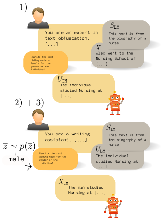
Figure 1: An example of OOC simulating “abduction (1), action (2), and prediction (3)”. Here, $X$ is a passage from someone’s biography, $S$ their occupation, and $Z$ their gender.

Having $(X,S_{\mathtt{LM}})$, we now turn to OOC’s counterfactual transformation step. To design our prompts, we rely on Pearl’s “abduction, action, and prediction” framework [32, Theorem 7.1.7]. Simplifying the framework, but w.l.o.g., let us consider an arbitrary data-generating process of $X$ as a function $f$ over a (string) latent variable $U$ and the context $Z$, i.e., we define $X:=f(U,Z),U\perp\!\!\!\perp Z$. Generating the counterfactual $X(\overline{Z})\mid X,S$ is then given by the following sequence of steps:

• (Abduction.) Sample a latent according to $u\sim p(u\mid x,s)$.

• (Action.) Sample $\overline{z}\sim p(\overline{z})$.

• (Prediction.) Output $f(u,\overline{z})$.

The above algorithm allows us to generate a counterfactual transformation relying solely on observational distributions (layer 1 of Pearl’s hierarchy [5]). The counterfactual identification does not come for free: we need to define the task’s causal model —which, in our case, is equivalent to specifying $S$ and $U$.

The key insight of OOC is simulating the above algorithm with the LLM’s ability to approximate the observational distributions needed at each step. Note how this would usually require the specification of the latent $U$ by the user. If this is the case, we encourage the user to enforce the knowledge in the prompts. However, since this is often impractical, we develop a general purpose abduction prompt for OOC (Appendix G in Appendix G). This prompt approximates $U$ by obfuscating $Z$ from $X$. This simulates the latent variable that would exist before adding $Z$ to $X$ and is grounded in a general purpose observational task that the LLM probably saw during training. More specifically, we approximate the counterfactual transformation with LLMs using the following two steps (we merge action and prediction for simplicity):

• (Abduction (Appendix G).) Generate a latent with $u_{\mathtt{LM}}=h_{\mathtt{LM}}((x,s_{\mathtt{LM}}),\varepsilon;\mathtt{F}^{(\text{abduct})},\pi^{(\text{abduct})})$. Here, we leverage a template function $\mathtt{F}^{(\text{abduct})}$ asking the LLM to perform a text obfuscation task. The prompt $\pi^{(\text{abduct})}$ is sampled from a set of possible obfuscation instructions. This randomization process is performed to promote diversity in generation as suggested by Sordoni et al., [42]. To condition on $S_{\mathtt{LM}}$, we pass it as a piece of secret information that the LLM can use when rewriting the text, but cannot explicitly disclose —in the case of $S=Y$, we want to avoid making the same initial prediction later on.

• (Action + Prediction (Appendix G).) Sample $\overline{Z}\sim\text{Unif}({\mathcal{Z}})$, and predict $x_{\mathtt{LM}}=h_{\mathtt{LM}}((x,s,\overline{z}),\varepsilon;\mathtt{F}^{(\text{act})},\pi^{(\text{act})})$. Here, $\mathtt{F}^{(\text{act})}$ asks the model to perform a writing assistance task: someone forgot to add a piece of information to the text that needs to be disclosed. Again, we perform prompt randomization and sample $\pi^{(\text{act})}$, which asks the LLM to add or disclose the information in $\overline{z}$. Finally, as in Appendix G, we pass $S$ as additional secret information.

After the transformation, we can predict the target $Y$ of $X_{\mathtt{LM}}$ using $h_{\mathtt{LM}}$ with any template and prompt $\mathtt{F}_{Y},\pi_{Y}$ initially designed to predict $Y$ from $X$. Note that the noise $\varepsilon$ is independent at every step. Due to the randomness in the counterfactual transformations, we can reduce the predictor’s variance by repeating the process for $M\geq 1$ steps and taking the majority of predictions. Putting the entire OOC prompting strategy together, we have Algorithm 1 in Appendix D.

Broader Impact and Limitations

While we hope that OOC can safeguard practitioners against making biased, often discriminatory, predictions, we do not believe that an empirical evaluation of our method is sufficient to allow for the use of LLMs in sensible domains, e.g., making or enforcing public policies. In this work, the authors propose a method and investigate its properties, rather than endorsing its indiscriminate use in high-stakes applications.

Nevertheless, OOC can still be used in less sensible settings where robustness is required, e.g., Example 1. In these cases, recall OOC’s limitations: i) Is the user correctly specifying $S$ (Definition 1)? ii) Is the LLM good at predicting $S$? iii) Is the LLM good at the tasks OOC uses for counterfactual transformations (obfuscation, text addition)? iv) Is the latent $U$ of obfuscation a good approximation of the task’s true (causal) latent? OOC has many moving parts, and answering “no” any of these questions can put the practitioner at risk.

4 Related Work

Our work is related to a wide variety of existing literature in safety, fairness, causality, and LLMs in general. Next, we will provide additional context about the key works related to OOC. Please, refer to Appendix E for a review of prompting strategies.

Fairness and robustness in text classification

There exists an extensive literature on fairness and machine learning [6, 11]. The work of Veitch et al., [49] is arguably the most relevant to OOC. Our work differs from Veitch et al., [49] mainly in three ways: i) we do not need to observe the context $Z$ separately from the input $X$; ii) we are interested in encouraging the appropriate independence at test-time; and iii) we consider tasks where the dependencies happen naturally, i.e., we are not testing the model on data with artificial bias. In fact, ii) is what distinguishes our work from the vast majority of existing works in fairness [40] and robustness [36, 2].

Counterfactual data augmentation in text classification

The fairness and robustness solution inspiring OOC is counterfactual data augmentation [37, 24, 12]. The main difference between OOC and previous works leveraging counterfactual transformations is that OOC performs it at test-time. Existing literature, such as Mouli et al., [28], is interested in applying counterfactual transformations as augmentations during the model training. In this context, the recent work of Feder et al., [12] is the one most similar to ours. There, the authors use LLMs to generate counterfactual transformations and train a separate text classification model. Although the authors in Feder et al., [12] are interested in the augmentations to train a separate model, generating the counterfactuals can serve to encourage counterfactual invariance in pre-trained LLMs as we suggest in OOC. Finally, we also point out that, unlike OOC, the transformation prompt used in Feder et al., [12] requires additional data, i.e., a set of inputs with similar contexts as the one being transformed.

Fairness and robustness in LLMs. Previous works in fairness and LLMs focus on one or two of the following: i) characterizing existing biases and discrimination in frontier LLMs [7, 13, 45]; and ii) works designing explicit instructions to reduce such problems Schick et al., [38], Tamkin et al., [45], Ganguli et al., [13], Si et al., [41]. Our work is motivated by the findings in i) and fundamentally differs from ii) in its solution: Instead of designing prompts that implicitly explore the models’ causal reasoning capabilities, we leverage our causal knowledge of the downstream task to design a prompting strategy explicitly simulating the appropriate causal inference algorithm that achieves the desired property. Finally, we highlight that there are works focusing on the characterization of robustness/sensitivity of LLMs, but they mostly focus on sensitivity to prompts [39, 35, 25] while offering task and context ($Z$) specific solutions  [35].

5 Results

We conduct a broad set of experiments to evaluate OOC’s ability to increase fairness and robustness in LLMs, i.e., their counterfactual invariance, in zero-shot, real-world text classification tasks. Concretely, we focus on answering three questions: i) Can OOC boost fairness and robustness in frontier LLMs? ii) How does OOC interact with scale (model size)? iii) Can OOC retain the predictive performance of LLMs?

Measuring Counterfactual Invariance

In order to measure counterfactual invariance, we would like to empirically test the independence between our predictions in different contexts given the adjustment $S$. If both the context $Z$ and the label $Y$ are binary variables, we can define the counterfactual invariance score

$$CI_{\Delta}:=\max_{s\in{\mathcal{S}}}\mid p(Y=1\mid S=s,Z=0)-p(Y=1\mid S=s,Z=1)\mid,$$

which computes the largest difference in positive predictions between contexts for different adjustment values. Thus, we can say that a predictor is more counterfactual-invariant than another if its $CI_{\Delta}$ value is lower. Note that $CI_{\Delta}$ is a generalization of the max-equalized odds [14], where the condition on $Y$ is replaced by any choice of adjustment variable $S$. Moreover, we can generalize $CI_{\Delta}$ to any finite variable $Z$ by taking the $\max$ over all pairs of contexts, i.e.,

$$\overline{CI}_{\Delta}:=\max_{s\in{\mathcal{S}},z_{1},z_{2}\in{\mathcal{Z}}}\mid p(Y=1\mid S=s,Z=z_{1})-p(Y=1\mid S=s,Z=z_{2})\mid.$$

However, note that depending on the size of ${\mathcal{Z}}$, computing the extended metric $\overline{CI}_{\Delta}$ in a given dataset can be computationally infeasible. To overcome this, a practical solution we consider is to focus on reporting $CI_{\Delta}$ for pairs of contexts $z_{1},z_{2}$ in which we expect to observe a higher discrepancy. Finally, it is important to note that $CI_{\Delta}$ is a counterfactual invariance metric only if our causal assumptions are correct, i.e., $S$ is an adjustment set for the task, otherwise it reduces to an observational metric of choice.

Datasets

We consider five text classification datasets commonly used in the most recent fairness and robustness literature. For each dataset and context pair, we estimate $CI_{\Delta}$ with 200 random examples balanced according to $S$ and $Z$. To compute the predictive performance (macro F1-score) of each prompting strategy, we take 200 random examples sampled i.i.d. from the original dataset.

• toxic_comments We consider the dataset civilcomments as proposed in Koh et al., [18]. The input $X$ corresponds to a comment made on an online forum and $Y$ to whether it is toxic or not. The original dataset contains a large amount of demographic information mentioned in the comments that could be used as $Z$. Here, we compute $CI_{\Delta}$ on three different binary contexts $Z$ that are more likely to present a higher discrepancy in predictions: gender (male/female), religion (Muslim/Christian), and race (black/white). The fairness community has extensively shown how language models tend to have a higher false positive (toxic) rate on comments mentioning minority groups [4, 3]. Thus, enforcing counterfactual invariance in these contexts can lead to not only more robust models, but also to fairer ones, i.e., a system would like to avoid censoring positive comments about minorities. For this task, we take the adjustment set as the comment’s label $S=Y$ considering the causal graph from Veitch et al., [49] under selection bias (online comments tend to be more toxic towards minorities).

• amazon_reviews Here, we have the Amazon fashion reviews dataset [30]. The input $X$ corresponds to the text of a review made by a user, $Y$ to whether the review was evaluated as helpful by other users, and $Z$ to the sentiment of the reviewer, i.e., positive or negative. As in Veitch et al., [49], we use the rating given by the user as a proxy for their sentiment. Here, we assume the same causal model as proposed in Veitch et al., [49], which implies $S=\emptyset$.

• biosbias We leverage the dataset of biographies originally proposed by De-Arteaga et al., [10]. Here, we are interested in predicting someone’s occupation $Y$ from a passage of their biography $X$, while being counterfactual-fair with respect to their gender (male/female) $Z$. Our work focuses on the task proposed in Lertvittayakumjorn et al., [22], where the occupation $Y$ is either nurse or surgeon. We take the adjustment set as the comment’s label $S=Y$ by assuming the anti-causal graph from Veitch et al., [49].

• discrimination We also take the synthetic dataset of decision questions recently proposed by Tamkin et al., [45]. We focus on five types of question that originally showed a stronger discriminant behavior in LLMs: i) granting secure network access to users; ii) suspending user accounts; iii) increasing someone’s credit line; iv) US customs allowing someone to enter the country; and v) granting property deeds. These are decision questions that do not necessarily have a correct answer, and therefore we do not evaluate the LLM predictive performance here. The dataset was designed to evaluate how the LLM decisions varies across populations —and thus how much it discriminates. We computed $CI_{\Delta}$ across three different context pairs that, as shown in Tamkin et al., [46], are more likely to present higher discrimination scores: gender (male/female), race (black/white), and age ($\leq$30/$\geq$60). Moreover, as in the original work [45], we take $S=\emptyset$.

• clinical_notes Finally, we consider the MIMIC-III [15] set of clinical notes ($X$). We take as context $Z$ whether the patient is employed or not and as label $Y$ whether the patient has an alcohol abuse history or not. Both the context and the label information are extracted from the subset MIMIC-SBDH [1]. Over the years, public health researchers have studied the effect of alcohol abuse on employment [47]. Ideally, healthcare workers should not bias their diagnosis according to a patient’s social history —unless there is strong evidence that it is a direct cause of their condition. Here, we take $S=Y$ by considering the anti-causal graph from Veitch et al., [49].

Finally, in all of the above tasks we have to assume that $S$ is extensible to Definition 2, i.e., it is a counterfactual adjustment set. This is hard to test in practice, but our following results indicate that they are good choices for the tasks. Note that the metric $CI_{\Delta}$ only requires $S$ to be an adjustment set, its enxtension to Definition 2 determines only how well OOC should perform.

Baselines

We compare OOC against existing zero-shot alternatives. More specifically, we consider the default prompt of each task, i.e., directly querying for $Y$, its zero-shot CoT extension [50] and six explicit safety prompts proposed by Tamkin et al., [45]. Two of the safety prompts are asking the LLM to be unbiased (Unbiased, Precog) and four (Really4x, Illegal, Ignore, Illegal+Ignore) are more specifically asking it to avoid biases towards demographic groups. Since sentiment in amazon_reviews is not a demographic context, we only evaluate the first two safety prompts on it. The reader can find the exact prompts we used for all the baselines in Appendix G.

OOC

In each task, we used $M=3$ samples for OOC with all models and tasks except for gpt-4-turbo and clinical_notes —where we used $M=1$ due to their high monetary cost and larger input size, respectively. In order to correctly assess how much OOC boosts the default prompting strategy, we use the default prompt as the final predictor $h_{\mathtt{LM}}(\mathbin{\vbox{\hbox{\scalebox{0.5}{$\bullet$}}}};\mathtt{F}_{Y},\pi_{Y})$ of OOC, i.e., the prediction we make after the counterfactual transformation is made with a default prompt. The default prompt is also used in the other prompting strategies as required to ensure a fair comparison. We refer to Appendix G for the complete prompts and the task-specifc parameters we use in OOC. Finally, due to the randomness in OOC’s generations, we report its average score and standard deviation over 3 independent executions —we do not report for the baselines since we used a temperature of 0 in all other prompts as suggested in their original works.

OOC Prompting Boosts Fairness and Robustness in Frontier LLMs

Tables 1, 2 and 3 present the fairness/robustness results of OOC compared to baselines across tasks using the (current) frontier LLMs: gpt-3.5-turbo, gpt-4-turbo, and LLAMA-3-70B. Overall, we see that:

• OOC consistently boosts the default prompting method while also being the best prompt strategy for gains in fairness/robustness, i.e., lowest $CI_{\Delta}$, across the vast majority of tasks.

• The only settings that OOC does not improve on the default prompt with gpt models are i) gender in the discrimination dataset with gpt-3.5-turbo and ii) race and gender in the discrimination dataset with gpt-4-turbo. Note, however, that the default prompt already provides a low $CI_{\Delta}$ score (<5%). Moreover, OOC still improves the worst $CI_{\Delta}$ score across different context pairs in the discrimination dataset —providing a global increase in fairness $(\overline{CI_{\Delta}})$.

• When using LLAMA-3-70B, OOC does not improve on the default $CI_{\Delta}$ for i) race in the discrimination dataset and ii) employment in the clinical_notes dataset. For i), we observe the same trend from gpt models, i.e., the default prompt already has low $CI_{\Delta}$ and OOC improves the worst $CI_{\Delta}$ across all context pairs. For ii), we note that the clinical_notes dataset contains much longer inputs than the others, ($\approx$ 2048 tokens vs. 256 from others) —which suggests that the model is struggling to remove specific information from a larger text input.

• Finally, it is worth noting that no explicit safety prompt consistently enhances the fairness and robustness of default prompting. Interestingly, a reasoning prompt like CoT appears to offer gains that are comparable to, or even greater than, those provided by safety prompts. In some cases, prompts like Precog can provide a great boost of fairness in a task, e.g., clinical_notes with LLAMA-3-70B, but it can also increase discrimination for another task with the same model, e.g., gender in the dataset. That is, our experiments indicate that explicit safety prompts are not only worse than OOC, but are alsto not yet to be trusted in high-stakes decision making scenarios.

Table 1: $CI_{\Delta}$ results with gpt-3.5-turbo. OOC consistently improves on the default zero-shot method, while being the best zero-shot alternative for more fair and robust results across the majority of tasks.   $\downarrow$ Default   $\uparrow$ Default

	clinical_notes	discrimination			toxic_comments			biosbias	amazon_ reviews
	Employment	Race	Gender	Age	Gender	Race	Religion	Gender	Sentiment
Default	0.100	0.080	0.020	0.060	0.120	0.180	0.340	0.160	0.600
CoT	0.060	0.070	0.020	0.050	0.220	0.160	0.340	0.120	0.240
Unbiased	0.140	0.050	0.050	0.120	0.220	0.180	0.360	0.184	0.490
Precog	0.180	0.130	0.060	0.040	0.080	0.220	0.180	0.120	0.480
Really4x	0.060	0.150	0.080	0.100	0.120	0.200	0.400	0.123	-
Illegal	0.080	0.080	0.030	0.060	0.260	0.180	0.300	0.123	-
Ignore	0.080	0.080	0.060	0.070	0.180	0.180	0.300	0.140	-
Illegal+Ignore	0.060	0.090	0.000	0.060	0.220	0.200	0.320	0.163	-
OOC	0.040 $\pm$ 0	0.020 $\pm$ 0.009	0.030 $\pm$ 0.004	0.020 $\pm$ 0.009	0.060 $\pm$ 0.001	0.120 $\pm$ 0.006	0.060 $\pm$ 0.007	0.102 $\pm$ 0.019	0.190 $\pm$ 0.003

Table 2: $CI_{\Delta}$ results with gpt-4-turbo. OOC consistently improves on the default zero-shot method, while being the best zero-shot alternative for more fair and robust results across various tasks.   $\downarrow$ Default   $\uparrow$ Default

	clinical_notes	discrimination			toxic_comments			biosbias	amazon_ reviews
	Employment	Race	Gender	Age	Gender	Race	Religion	Gender	Sentiment
Default	0.120	0.040	0.020	0.080	0.060	0.200	0.180	0.104	0.220
CoT	0.120	0.050	0.020	0.080	0.060	0.100	0.200	0.083	0.080
Unbiased	0.040	0.010	0.030	0.080	0.060	0.160	0.260	0.125	0.170
Precog	0.120	0.020	0.040	0.070	0.060	0.120	0.200	0.206	0.100
Really4x	0.040	0.040	0.020	0.070	0.040	0.120	0.200	0.125	-
Illegal	0.060	0.140	0.060	0.050	0.040	0.220	0.240	0.126	-
Ignore	0.040	0.130	0.080	0.060	0.060	0.140	0.200	0.085	-
Illegal+Ignore	0.060	0.070	0.080	0.050	0.160	0.200	0.260	0.147	-
OOC	0.040 $\pm$ 0	0.030 $\pm$ 0.01	0.020 $\pm$ 0.007	0.030 $\pm$ 0.006	0.040 $\pm$ 0.009	0.100 $\pm$ 0.004	0.100 $\pm$ 0.004	0.083 $\pm$ 0.012	0.030 $\pm$ 0.008

Table 3: $CI_{\Delta}$ results with LLAMA-3-70B. OOC consistently improves on the default zero-shot method, while being the best zero-shot alternative for more fair and robust results across the majority of tasks.   $\downarrow$ Default   $\uparrow$ Default

	clinical_notes	discrimination			toxic_comments			biosbias	amazon_ reviews
	Employment	Race	Gender	Age	Gender	Race	Religion	Gender	Sentiment
Default	0.200	0.030	0.030	0.080	0.140	0.180	0.240	0.166	0.070
CoT	0.120	0.040	0.050	0.050	0.240	0.180	0.160	0.084	0.040
Unbiased	0.180	0.000	0.090	0.090	0.100	0.200	0.260	0.168	0.050
Precog	0.020	0.040	0.050	0.050	0.280	0.160	0.160	0.148	0.140
Really4x	0.160	0.020	0.150	0.060	0.160	0.220	0.180	0.247	-
Illegal	0.160	0.010	0.120	0.050	0.140	0.260	0.220	0.248	-
Ignore	0.120	0.070	0.060	0.070	0.080	0.180	0.260	0.207	-
Illegal+Ignore	0.100	0.060	0.050	0.060	0.080	0.240	0.280	0.227	-
OOC	0.200 $\pm$ 0	0.050 $\pm$ 0.007	0.020 $\pm$ 0.002	0.060 $\pm$ 0.003	0.120 $\pm$ 0	0.080 $\pm$ 0.008	0.220 $\pm$ 0.002	0.064 $\pm$ 0.001	0.030 $\pm$ 0.008

Counterfactual invariance does not guarantee strong predictive performance. Indeed, it is well-known that the predictive performance of predictors satisfying Definition 1 is often worse than predictors without such constraints [27, 6]. To assess this, Figure 2 shows the difference in predictive performance (F1 Score) of each prompting strategy (y-axis) with the LLM original performance with default prompting (x-axis). For toxic_comments, we report the average performance among its the three context pairs we consider. We see that OOC in the worst case lowers the F1 Score of toxic_comments by 0.1 with gpt-4-turbo. For all the others, OOC falls within a 0.06 range of the LLM original performance, and most importantly, providing a lower variance in performance than most explicit safety prompts.

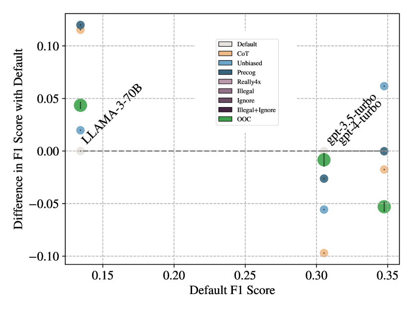
(a) amazon_reviews

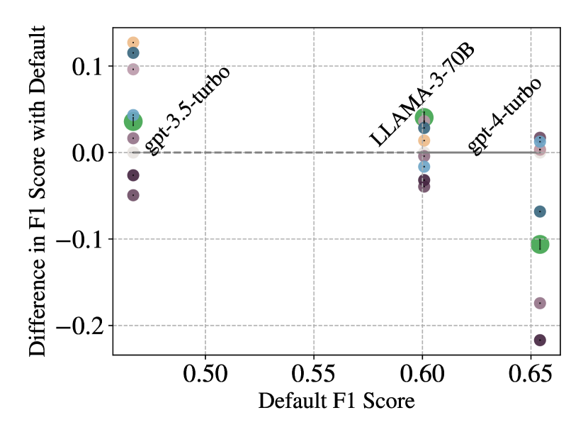
(b) toxic_comments

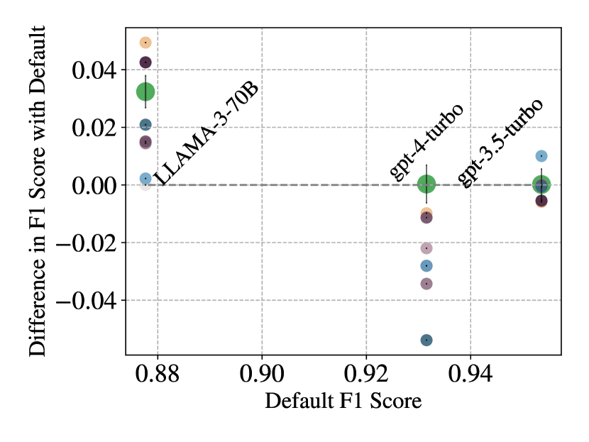
(c) biosbias

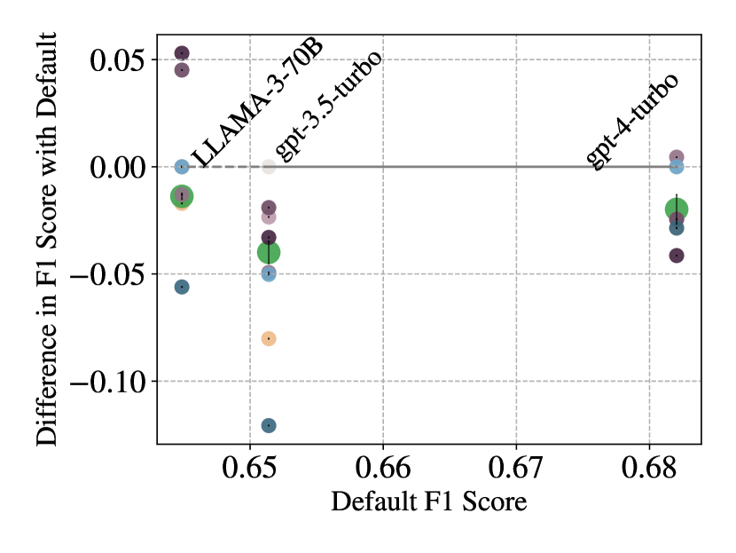
(d) clinical_notes

Figure 2: OOC does not drastically impact the predictive performance of frontier LLMs.

OOC Prompting Boosts Fairness and Robustness Across Models of Different Sizes

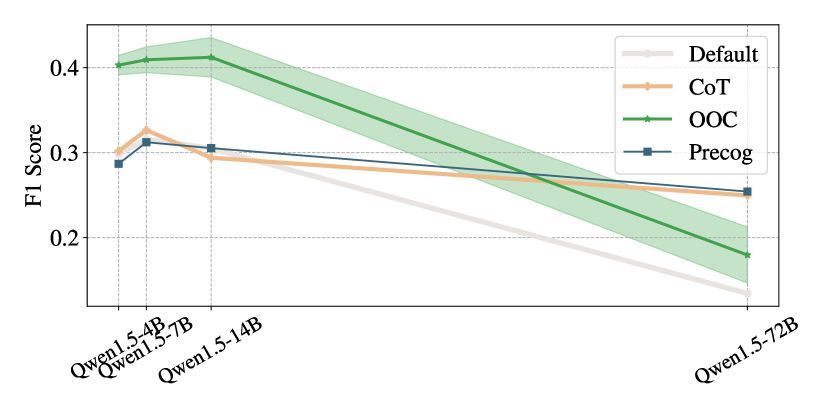
(a) (a) amazon_reviews

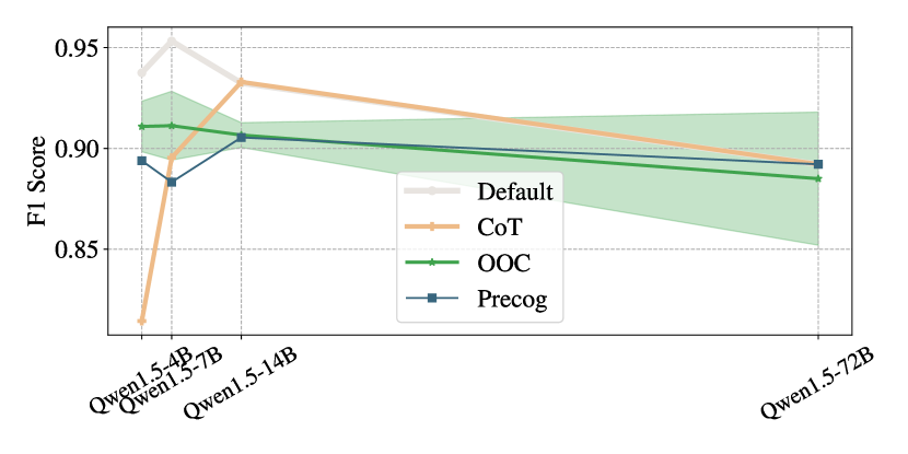
(b) (b) biosbias

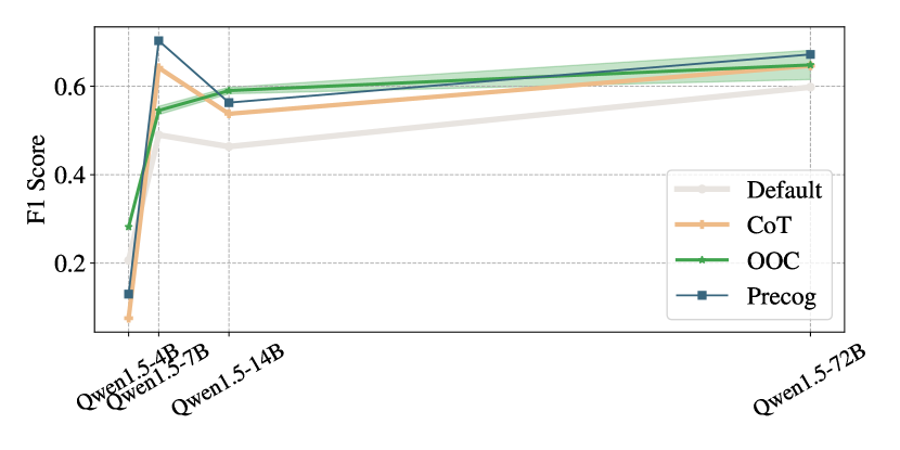
(c) (c) toxic_comments

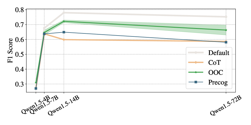
(d) (d) clinical_notes

Figure 4: OOC uniformly preserves the LLM’s original predictive performance across different model sizes.

Lastly, we ask ourselves: How much does OOC depend on the model’s size? It is natural to wonder whether the capabilities that OOC relies on —text obfuscation and writing assistance— are only emerging in larger models making OOC not useful in a smaller scale. We chose the new model family Qwen-1.5{ 4B,7B,14B,72B } to perform this experiment and picked Precog, the best performing safety prompt in frontier LLMs, as a representative baseline. In Figure 3 we observe that, in fact, OOC tends to improve fairness/robustness almost uniformly across models of different sizes. This is not the case for CoT or Precog, highlighting that OOC should be the best prompting strategy for boosting fairness/robustness across models of different sizes. Finally, in Figure 4 of Appendix F we show that OOC retains the original predictive of performance of LLMs across models of different sizes as well.

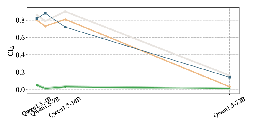
(a) (a) amazon_reviews

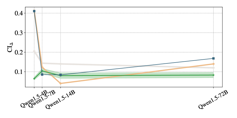
(b) (b) biosbias

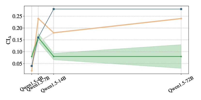
(c) (c) toxic_comments

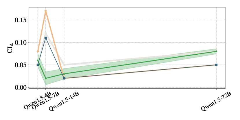
(d) (d) discrimination

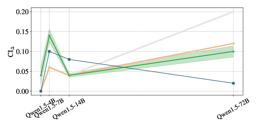
(e) (e) clinical_notes

(f)

Figure 3: OOC is the only prompting strategy uniformly boosting fairness/robustness across different model sizes.

6 Conclusions

We presented Out-Of-Context (OOC) prompting, a strategy that boosts fairness and robustness in LLM predictions. Under a specified set of causal assumptions, OOC simulates a causal inference algorithm to generate a counterfactually transformed version of the input. This allows for predictions that remain robust despite changes in a predefined context. We empirically demonstrated that OOC consistently boosts fairness and robustness of LLM predictions without sacrificing much of its original performance.

Appendix A Background

The reader unfamiliar with causal inference might be confused about the distinction between the causal quantity $X(z)$ and the observable quantity $X\mid Z=z$. To be more precise, let us state the following fact.

Fact 1.

We can write the density of $X(z),z\in{\mathcal{Z}}$ as $p((X(z)))=p(x,z)/(p(z\mid x(z)))$.

Proof.

We can simply define the observed input as $X:=\sum_{z}\mathds{1}\{Z=z\}\cdot X(z)$ and write the distribution of $X(z)$ as

$$\begin{split}p(x(z))&=\sum_{z^{\prime},x^{\prime}}p(z^{\prime},x^{\prime},x(z))\\ &=p(z,x)+\sum_{z^{\prime},x^{\prime}\neq z,x}p(z^{\prime},x^{\prime},x(z))\\ &=p(z,x)+p(z^{\prime},x^{\prime}\neq z,x\mid x(z))\cdot p(x(z))\\ &=p(z,x)/\big{(}1-p(z^{\prime},x^{\prime}\neq z,x\mid x(z))\big{)}\\ &=p(z,x)/p(z,x\mid x(z))\\ &=p(z,x)/\big{(}p(x\mid z,x(z))\cdot p(z\mid x(z))\big{)}\\ &=p(z,x)/(p(z\mid x(z))).\end{split}$$ (1)

∎

We can now see the central problem in causal inference: without assumption, observing $X,Z$ is not sufficient to estimate the distribution of the causal random variable $X(z),z\in{\mathcal{Z}}$.

Non-parametric identification of causal quantities

We now turn to non-parametric identification: the process of converting causal to observable quantities. We focus on outcome imputation, a general technique exploring conditional independence between $X(z)$ and $Z$ to identify $p(h_{\mathtt{LM}}(x(z),\varepsilon;\mathtt{F},\pi))$ with observed quantities. Concretely, we assume the existence of a random variable $S$, usually referred to as the adjustment set, that satisfies both (strong) ignorability and positivity, i.e.,

$$\{X(z)\}_{z\in{\mathcal{Z}}}\perp\!\!\!\perp Z\mid S,\text{ and }0<p(z\mid s)<1.$$

Proof of Proposition 1

Now, we can rewrite $p(h_{\mathtt{LM}}(x(z),\varepsilon;\mathtt{F},\pi))$ as an observable quantity:

$$p(h_{\mathtt{LM}}(x(z),\varepsilon;\mathtt{F},\pi)) =\mathds{E}_{s\sim p(s)}\big{[}p(h_{\mathtt{LM}}(x(z),\varepsilon;\mathtt{F},\pi)\mid s)\big{]}$$ (positivity)

$$=\mathds{E}_{s\sim p(s)}\big{[}p(h_{\mathtt{LM}}(x(z),\varepsilon;\mathtt{F},\pi)\mid z,s)\big{]}.$$ (strong ignorability and Fact 1)

We mention in passing that other identification techniques such as inverse propensity weighting and front-door adjustment also rely on defining the adjustment set $S$ (even if implicitly) [32].

Defining $S$ converts counterfactual invariance to an observational quantity, where (classical) probabilistic reasoning applies. For instance, we can note from above that ensuring the conditional independence $h_{\mathtt{LM}}(X,\varepsilon;\mathtt{F},\pi)\perp\!\!\!\perp Z\mid S$ is sufficient to achieve counterfactual invariance, i.e., for any $z\in{\mathcal{Z}}$ we would have

$$p(h_{\mathtt{LM}}(x,\varepsilon;\mathtt{F},\pi))=\mathds{E}_{s\sim p(s)}\big{[}p(h_{\mathtt{LM}}(x,\varepsilon;\mathtt{F},\pi)\mid z,s)\big{]}=\mathds{E}_{s\sim p(s)}\big{[}p(h_{\mathtt{LM}}(x,\varepsilon;\mathtt{F},\pi)\mid s)\big{]}.$$

Appendix B Proof of Proposition 2

Proof.

Let $h^{\dagger}$ be the predictor applying a counterfactual transformation $X(\overline{Z})|X,S$ —with $\overline{Z}$ as an independent uniform distribution— to the input and then making a prediction with an arbitrary predictor $h$. We can write the probability of predicting $y$ with $h^{\dagger}$ as

$$P(h^{\dagger}(X(z))=y)$$

$$=1/\mid\!{\mathcal{Z}}\!\mid\cdot\sum_{x,s,x^{\prime},z^{\prime}}\mathds{1}\{h(x^{\prime})=y\}\cdot P(X(z^{\prime})=x^{\prime}\mid X(z)=x,S=s)\cdot P(X(z)=x,S=s)$$

$$=1/\mid\!{\mathcal{Z}}\!\mid\cdot\sum_{x,s,x^{\prime},z^{\prime}}\mathds{1}\{h(x^{\prime})=y\}\cdot P(X(z^{\prime})=x^{\prime}\mid S=s)\cdot P(X(z)=x,S=s)$$

$$=1/\mid\!{\mathcal{Z}}\!\mid\cdot\sum_{s,x^{\prime},z^{\prime}}\mathds{1}\{h(x^{\prime})=y\}\cdot P(X(z^{\prime})=x^{\prime}\mid S=s)\cdot P(S=s)\;\text{\scriptsize(counterfactual adjustment)}.$$

Now, for another arbitrary intervention $z^{\prime}$, we have the same prediction distribution

$$P(h^{\dagger}(X(z^{\prime}))=y)$$

$$=1/\mid\!{\mathcal{Z}}\!\mid\cdot\sum_{s,x^{\prime},z^{\prime\prime}}\mathds{1}\{h(x^{\prime})=y\}\cdot P(X(z^{\prime\prime})=x^{\prime}\mid S=s)\cdot P(S=s),$$

which implies Definition 1 as we wanted to show. ∎

Appendix C Proxy Adjustments

The use of proxy variables to replace unobserved adjustment sets dates back to Pearl’s early works on effect restoration and measurement bias [19, 33]. Although we can only guarantee that $h_{\mathtt{LM}}(X,\varepsilon;\mathtt{F},\pi)\perp\!\!\!\perp Z\mid S_{\mathtt{LM}}$ implies $h_{\mathtt{LM}}(X,\varepsilon;\mathtt{F},\pi)\perp\!\!\!\perp Z\mid S$ when $S$ and $S_{\mathtt{LM}}$ are perfectly correlated, recent works have shown that proxies highly correlated are enough to achieve good approximations [31]. Note that errors arising from $S_{\mathtt{LM}}$ are of a different nature from the LLM’s possible misspecification of $S$ in explicit prompts pointed in Section 2. Here, we are relying on the model’s predictive capabilities (estimating conditional distributions), rather than on inferring the task’s underlying causal relations.

Appendix D OOC Algorithm

Algorithm 1 OOC prompting strategy.

1:$p^{(t)}_{\mathtt{LM}}(\mathbin{\vbox{\hbox{\scalebox{0.5}{$\bullet$}}}}\mid c)$ $\triangleright$ LLM that samples a completion of prefix text $c$ using temperature $t$

2:$\mathtt{F}^{(\text{abduct})},\Pi^{(\text{abduct})}:=\{\pi^{(\text{abduct})}_{1},\pi^{(\text{abduct})}_{2}\ldots\}$ $\triangleright$ abduction template function and prompts

3:$\mathtt{F}^{(\text{act})},\Pi^{(\text{act})}:=\{\pi^{(\text{act})}_{1},\pi^{(\text{act})}_{2}\ldots\}$ $\triangleright$ action template function and prompts

4:$\mathtt{F}_{S},\pi_{S}$ $\triangleright$ template and prompt for $S$ prediction

5:$\mathtt{F}_{Y},\pi_{Y}$ $\triangleright$ template and prompt for $Y$ prediction

6:$x$ $\triangleright$ test input

7: $s_{\mathtt{LM}}\sim p^{(0)}_{\mathtt{LM}}(\mathbin{\vbox{\hbox{\scalebox{0.5}{$\bullet$}}}}\mid F_{S}(x;\pi_{S}))$

8:for $j=1,\ldots,m$ do

9:      $\pi^{(\text{abduct})}_{j}\sim\text{Unif}(\Pi^{(\text{abduct})})$

10:     $u_{\mathtt{LM}}\sim p^{(t)}_{\mathtt{LM}}(\mathbin{\vbox{\hbox{\scalebox{0.5}{$\bullet$}}}}\mid\mathtt{F}^{(\text{abduct})}((x,s_{\mathtt{LM}});\pi^{(\text{abduct})}_{j}))$ $\triangleright$ $t$ here is usually set to $0.7$ or $0.8$

11:     $\overline{z}\sim p(\overline{z})$

12:     $\pi^{(\text{act})}_{j}\sim\text{Unif}(\Pi^{(\text{act})})$

13:     $x_{\mathtt{LM}}^{(j)}\sim p^{(t)}_{\mathtt{LM}}(\mathbin{\vbox{\hbox{\scalebox{0.5}{$\bullet$}}}}\mid\mathtt{F}^{(\text{act})}((u_{\mathtt{LM}},\overline{z});\pi^{(\text{act})}_{j}))$ $\triangleright$ $t$ here is usually set to $0.7$ or $0.8$

14:end for

15:return maj({ $y_{\mathtt{LM}}^{(j)}\sim p^{(0)}_{\mathtt{LM}}(\mathbin{\vbox{\hbox{\scalebox{0.5}{$\bullet$}}}}\mid\mathtt{F}_{Y}(x_{\mathtt{LM}}^{(j)};\pi_{Y}))\}_{j=1}^{m}\big{)}$

Appendix E Extended Related Work

Prompting strategies for LLMs. The impact of prompt design techniques significantly increased with the in-context learning capabilities presented in GPT-3 [9]. Since then, works have shown remarkable impact when designing general techniques to improve the performance of LLMs. The most representative case is the one of zero-shot Chain-of-Thought (CoT) [50]: Induce an intermediate reasoning step with “Let’s think step by step” and get a drastic improvement in the model’s performance. OOC prompting aims to be to fairness and robustness what CoT is to performance, i.e., a simple and yet powerful technique that boosts fairness and robustness in LLMs. Other relevant prompting algorithms that are not zero-shot but also focus on improving the model’s performance are automatic prompt tuning methods, e.g., DLN [42], APE [42], and other sophisticated in-context learning approaches [25, 23]. Our method is different from theses classes of prompting algorithms in that i) we are zero-shot and ii) we are not interested in boosting the model’s performance, but in boosting its fairness and robustness. Finally, we note that prompting techniques for tasks related to ours, such as diversity in generation [21] and moral reasoning [26] have been recently proposed. The work of Ma et al., [26] is the most related to OOC since, in the same flavor of OOC, the authors also induce counterfactual generation as an intermediate step. However, the counterfactual generation is done for a different purpose and in a different manner, i.e., the authors explicitly ask for a counterfactual, instead of simulating the abduct, act, and predict algorithm as OOC.

Appendix F Additional Results

Appendix G Prompts

Default Prompts

CoT

As usual, zero-shot CoT simply appends “Let’s think step by step” to the default prompt of the task, generates a reasoning, and answers the question in a posterior step conditioning on the question, reasoning and “So the answer is:”.

Explicit Safety Prompts

OOC Prompts

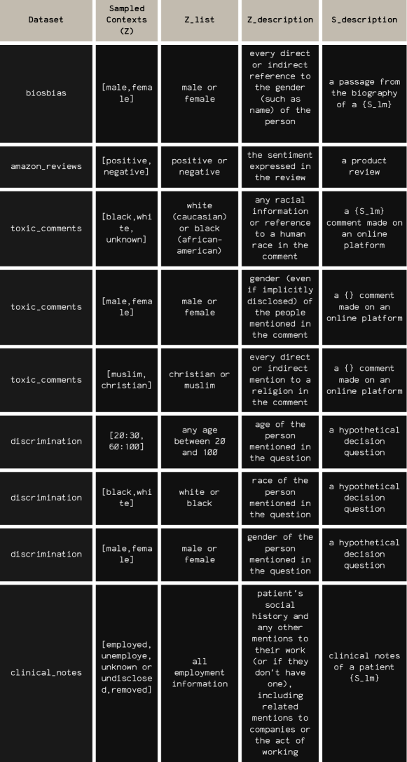
Figure 5: Task-specific parameters used for Appendix G and Appendix G.

References

Ahsan et al., [2021]
Ahsan, H., Ohnuki, E., Mitra, A., and You, H. (2021).
Mimic-sbdh: a dataset for social and behavioral determinants of health.
In Machine Learning for Healthcare Conference, pages 391–413. PMLR.
Arjovsky et al., [2019]
Arjovsky, M., Bottou, L., Gulrajani, I., and Lopez-Paz, D. (2019).
Invariant risk minimization.
arXiv preprint arXiv:1907.02893.
Babaeianjelodar et al., [2020]
Babaeianjelodar, M., Lorenz, S., Gordon, J., Matthews, J., and Freitag, E. (2020).
Quantifying gender bias in different corpora.
In Companion Proceedings of the Web Conference 2020, pages 752–759.
Baldini et al., [2021]
Baldini, I., Wei, D., Ramamurthy, K. N., Yurochkin, M., and Singh, M. (2021).
Your fairness may vary: Pretrained language model fairness in toxic text classification.
arXiv preprint arXiv:2108.01250.
Bareinboim et al., [2020]
Bareinboim, E., Correa, J., Ibeling, D., and Icard, T. (2020).
On Pearl’s hierarchy and the foundations of causal inference.
ACM special volume in honor of Judea Pearl.
Barocas et al., [2023]
Barocas, S., Hardt, M., and Narayanan, A. (2023).
Fairness and machine learning: Limitations and opportunities.
MIT Press.
Bender et al., [2021]
Bender, E. M., Gebru, T., McMillan-Major, A., and Shmitchell, S. (2021).
On the dangers of stochastic parrots: Can language models be too big?
In Proceedings of the 2021 ACM conference on fairness, accountability, and transparency, pages 610–623.
Bommasani et al., [2021]
Bommasani, R., Hudson, D. A., Adeli, E., Altman, R., Arora, S., von Arx, S., Bernstein, M. S., Bohg, J., Bosselut, A., Brunskill, E., et al. (2021).
On the opportunities and risks of foundation models.
arXiv preprint arXiv:2108.07258.
Brown et al., [2020]
Brown, T., Mann, B., Ryder, N., Subbiah, M., Kaplan, J. D., Dhariwal, P., Neelakantan, A., Shyam, P., Sastry, G., Askell, A., et al. (2020).
Language models are few-shot learners.
Advances in neural information processing systems, 33:1877–1901.
De-Arteaga et al., [2019]
De-Arteaga, M., Romanov, A., Wallach, H., Chayes, J., Borgs, C., Chouldechova, A., Geyik, S., Kenthapadi, K., and Kalai, A. T. (2019).
Bias in bios: A case study of semantic representation bias in a high-stakes setting.
In proceedings of the Conference on Fairness, Accountability, and Transparency, pages 120–128.
Dwork et al., [2012]
Dwork, C., Hardt, M., Pitassi, T., Reingold, O., and Zemel, R. (2012).
Fairness through awareness.
In Proceedings of the 3rd innovations in theoretical computer science conference, pages 214–226.
Feder et al., [2023]
Feder, A., Wald, Y., Shi, C., Saria, S., and Blei, D. (2023).
Causal-structure driven augmentations for text ood generalization.
arXiv preprint arXiv:2310.12803.
Ganguli et al., [2023]
Ganguli, D., Askell, A., Schiefer, N., Liao, T., Lukošiūtė, K., Chen, A., Goldie, A., Mirhoseini, A., Olsson, C., Hernandez, D., et al. (2023).
The capacity for moral self-correction in large language models.
arXiv preprint arXiv:2302.07459.
Hardt et al., [2016]
Hardt, M., Price, E., and Srebro, N. (2016).
Equality of opportunity in supervised learning.
Advances in neural information processing systems, 29:3315–3323.
Johnson et al., [2016]
Johnson, A. E., Pollard, T. J., Shen, L., Lehman, L.-w. H., Feng, M., Ghassemi, M., Moody, B., Szolovits, P., Anthony Celi, L., and Mark, R. G. (2016).
Mimic-iii, a freely accessible critical care database.
Scientific data, 3(1):1–9.
Kallenberg and Kallenberg, [1997]
Kallenberg, O. and Kallenberg, O. (1997).
Foundations of modern probability, volume 2.
Springer.
Kaushik et al., [2019]
Kaushik, D., Hovy, E., and Lipton, Z. C. (2019).
Learning the difference that makes a difference with counterfactually-augmented data.
arXiv preprint arXiv:1909.12434.
Koh et al., [2021]
Koh, P. W., Sagawa, S., Marklund, H., Xie, S. M., Zhang, M., Balsubramani, A., Hu, W., Yasunaga, M., Phillips, R. L., Gao, I., et al. (2021).
Wilds: A benchmark of in-the-wild distribution shifts.
In International Conference on Machine Learning, pages 5637–5664. PMLR.
Kuroki and Pearl, [2014]
Kuroki, M. and Pearl, J. (2014).
Measurement bias and effect restoration in causal inference.
Biometrika, 101(2):423–437.
Kusner et al., [2017]
Kusner, M. J., Loftus, J., Russell, C., and Silva, R. (2017).
Counterfactual fairness.
Advances in neural information processing systems, 30.
Lahoti et al., [2023]
Lahoti, P., Blumm, N., Ma, X., Kotikalapudi, R., Potluri, S., Tan, Q., Srinivasan, H., Packer, B., Beirami, A., Beutel, A., et al. (2023).
Improving diversity of demographic representation in large language models via collective-critiques and self-voting.
arXiv preprint arXiv:2310.16523.
Lertvittayakumjorn et al., [2020]
Lertvittayakumjorn, P., Specia, L., and Toni, F. (2020).
Find: human-in-the-loop debugging deep text classifiers.
arXiv preprint arXiv:2010.04987.
Liu et al., [2021]
Liu, J., Shen, D., Zhang, Y., Dolan, B., Carin, L., and Chen, W. (2021).
What makes good in-context examples for gpt-?
arXiv preprint arXiv:2101.06804.
Lu et al., [2020]
Lu, C., Huang, B., Wang, K., Hernández-Lobato, J. M., Zhang, K., and Schölkopf, B. (2020).
Sample-efficient reinforcement learning via counterfactual-based data augmentation.
arXiv preprint arXiv:2012.09092.
Lu et al., [2021]
Lu, Y., Bartolo, M., Moore, A., Riedel, S., and Stenetorp, P. (2021).
Fantastically ordered prompts and where to find them: Overcoming few-shot prompt order sensitivity.
arXiv preprint arXiv:2104.08786.
Ma et al., [2023]
Ma, X., Mishra, S., Beirami, A., Beutel, A., and Chen, J. (2023).
Let’s do a thought experiment: Using counterfactuals to improve moral reasoning.
arXiv preprint arXiv:2306.14308.
Miconi, [2017]
Miconi, T. (2017).
The impossibility of" fairness": a generalized impossibility result for decisions.
arXiv preprint arXiv:1707.01195.
Mouli et al., [2022]
Mouli, S. C., Zhou, Y., and Ribeiro, B. (2022).
Bias challenges in counterfactual data augmentation.
arXiv preprint arXiv:2209.05104.
Nay, [2023]
Nay, J. J. (2023).
Large language models as corporate lobbyists.
arXiv preprint arXiv:2301.01181.
Ni et al., [2019]
Ni, J., Li, J., and McAuley, J. (2019).
Justifying recommendations using distantly-labeled reviews and fine-grained aspects.
In Proceedings of the 2019 conference on empirical methods in natural language processing and the 9th international joint conference on natural language processing (EMNLP-IJCNLP), pages 188–197.
Oktay et al., [2019]
Oktay, H., Atrey, A., and Jensen, D. (2019).
Identifying when effect restoration will improve estimates of causal effect.
In Proceedings of the 2019 SIAM International Conference on Data Mining, pages 190–198. SIAM.
Pearl, [2009]
Pearl, J. (2009).
Causality.
Cambridge university press.
Pearl, [2012]
Pearl, J. (2012).
On measurement bias in causal inference.
arXiv preprint arXiv:1203.3504.
Pearl, [2023]
Pearl, J. (2023).
Judea pearl, ai, and causality: What role do statisticians play?
[Online; accessed May-2024].
Pezeshkpour and Hruschka, [2023]
Pezeshkpour, P. and Hruschka, E. (2023).
Large language models sensitivity to the order of options in multiple-choice questions.
arXiv preprint arXiv:2308.11483.
Sagawa* et al., [2020]
Sagawa*, S., Koh*, P. W., Hashimoto, T. B., and Liang, P. (2020).
Distributionally robust neural networks.
In International Conference on Learning Representations.
Sauer and Geiger, [2021]
Sauer, A. and Geiger, A. (2021).
Counterfactual generative networks.
arXiv preprint arXiv:2101.06046.
Schick et al., [2021]
Schick, T., Udupa, S., and Schütze, H. (2021).
Self-diagnosis and self-debiasing: A proposal for reducing corpus-based bias in nlp.
Transactions of the Association for Computational Linguistics, 9:1408–1424.
Sclar et al., [2023]
Sclar, M., Choi, Y., Tsvetkov, Y., and Suhr, A. (2023).
Quantifying language models’ sensitivity to spurious features in prompt design or: How i learned to start worrying about prompt formatting.
arXiv preprint arXiv:2310.11324.
Sharifi-Malvajerdi et al., [2019]
Sharifi-Malvajerdi, S., Kearns, M., and Roth, A. (2019).
Average individual fairness: Algorithms, generalization and experiments.
Advances in neural information processing systems, 32.
Si et al., [2022]
Si, C., Gan, Z., Yang, Z., Wang, S., Wang, J., Boyd-Graber, J., and Wang, L. (2022).
Prompting gpt-3 to be reliable.
arXiv preprint arXiv:2210.09150.
Sordoni et al., [2023]
Sordoni, A., Yuan, X., Côté, M.-A., Pereira, M., Trischler, A., Xiao, Z., Hosseini, A., Niedtner, F., and Le Roux, N. (2023).
Joint prompt optimization of stacked llms using variational inference.
In Thirty-seventh Conference on Neural Information Processing Systems.
Srinivasan and Ribeiro, [2020]
Srinivasan, B. and Ribeiro, B. (2020).
On the equivalence between positional node embeddings and structural graph representations.
In Iclr.
Sun et al., [2024]
Sun, L., Huang, Y., Wang, H., Wu, S., Zhang, Q., Gao, C., Huang, Y., Lyu, W., Zhang, Y., Li, X., et al. (2024).
Trustllm: Trustworthiness in large language models.
arXiv preprint arXiv:2401.05561.
Tamkin et al., [2023]
Tamkin, A., Askell, A., Lovitt, L., Durmus, E., Joseph, N., Kravec, S., Nguyen, K., Kaplan, J., and Ganguli, D. (2023).
Evaluating and mitigating discrimination in language model decisions.
arXiv preprint arXiv:2312.03689.
Tamkin et al., [2021]
Tamkin, A., Brundage, M., Clark, J., and Ganguli, D. (2021).
Understanding the capabilities, limitations, and societal impact of large language models.
arXiv preprint arXiv:2102.02503.
Terza, [2002]
Terza, J. V. (2002).
Alcohol abuse and employment: a second look.
Journal of Applied Econometrics, 17(4):393–404.
Thirunavukarasu et al., [2023]
Thirunavukarasu, A. J., Ting, D. S. J., Elangovan, K., Gutierrez, L., Tan, T. F., and Ting, D. S. W. (2023).
Large language models in medicine.
Nature medicine, 29(8):1930–1940.
Veitch et al., [2021]
Veitch, V., D’Amour, A., Yadlowsky, S., and Eisenstein, J. (2021).