Stabilization of a Quadrotor via Energy Shaping

Abstract

Stabilization of a quadrotor without a controller based on cascade structure is a challenging problem. Besides, due to the dynamics and the number of underactuation, an energy shaping controller has not been designed in 3D for a quadrotor. This paper presents a novel solution to the potential energy shaping problem for a quadrotor utilizing the Interconnection and Damping Assignment Passivity Based Control (IDA-PBC) approach. For the first time, we extend the solution of PDEs from the 2D case to the full 3D scenario. This advancement seems to be a significant step forward for stabilization of underactuated aerial vehicles without a cascade controller. The results are verified via simulation on a typical quadrotor.

, and

1 Introduction

The control of underactuated mechanical systems has been pivotal in various fields, including robotics, mechanics, and aerospace. The Interconnection and Damping Assignment Passivity-Based Control (IDA-PBC) methodology involves designing the control action such that the closed-loop dynamics preserve the port-Hamiltonian structure and are characterized by a desired total energy. The key advantages of IDA-PBC are the interpretability of the closed-loop dynamics in terms of mechanical structure and its passivity properties [1, 2, 3].

This paper addresses a significant advancement in the field of control methodologies for underactuated mechanical systems, specifically focusing on a quadrotor unmanned aerial vehicle (UAV). While previous research has primarily tackled partial differential equations (PDEs) in the two-dimensional (2D) case for such systems, our work successfully extends these solutions to the full three-dimensional (3D) scenario. By leveraging the IDA-PBC approach, we introduce a novel method for shaping the potential energy of a quadrotor with an underactuated degree of two. This development marks a critical milestone as it is the first instance where the potential shaping problem for a 3D quadrotor has been effectively solved using IDA-PBC.

Previous studies, such as [4, 5, 6, 7], have demonstrated the robustness and practical applicability of IDA-PBC in reshaping the physical properties of a quadrotor for better Aerial Physical Interaction (APhI) performances. These works have primarily focused on sensor noise robustness and evaluated the control method through experimental scenarios involving physical human-quadrotor interaction and surface inspection tasks. Another notable research effort [8] extended the IDA-PBC framework to control the entire physical characteristics of a quadrotor, thereby achieving desired interactive behaviors between the UAV and its environment through energy shaping and damping injection.

In this context, our contribution is particularly noteworthy as it not only confirms the applicability of IDA-PBC in a more complex 3D environment but also provides a comprehensive solution to the potential energy shaping problem, which has not been fully addressed in previous works. This paper provides detailed derivations of the necessary PDEs and their solutions, demonstrating the stabilization of equilibrium points (EPs) in the quadrotor’s dynamic equations. Additionally, we highlight the steps to ensure the positive definiteness of the Hessian of the potential function around the desired equilibrium, thereby guaranteeing the stability of the proposed control law.

2 Mathematical requirements

In this section, IDA-PBC method and the dynamic of a quadrotor are reviewed.

2.1 IDA-PBC

The equations of a $n$-DOF mechanical system in port Hamiltonian form are [9, 10]

$$\begin{bmatrix}\dot{q}\\ \dot{p}\end{bmatrix}=\begin{bmatrix}0_{n\times n}&I_{n}\\ -I_{n}&0_{n\times n}\end{bmatrix}\begin{bmatrix}\nabla_{q}H\\ \nabla_{p}H\end{bmatrix}+\begin{bmatrix}0_{n\times m}\\ G(q)\end{bmatrix}u,$$ (1)

where $q,p\in\mathbb{R}^{n}$ denote position and momentum, respectively, $H(q,p)=\frac{1}{2}p^{T}M^{-1}(q)p+V(q)$ in which $0<M\in\mathbb{R}^{n\times n}$ is the positive definite inertia matrix and $V(q)$ is the potential energy, $G(q)\in\mathbb{R}^{n\times m}$ denotes full rank input mapping matrix, and $u\in\mathbb{R}^{m}$ is the control input. Using the following control law

$$u =(G^{T}G)^{-1}G^{T}(\nabla_{q}H-M_{d}M^{-1}\nabla_{q}H_{d}+J_{2}\nabla_{p}H_{d})$$

$$-K_{v}G^{T}\nabla_{p}H_{d},$$ (2)

in which the desired inertia matrix and potential function are derived from the following PDEs, respectively,

$$G^{\bot}\{\nabla_{q}\big{(}p^{T}M^{-1}(q)p\big{)}-M_{d}M^{-1}(q)\nabla_{q}\big{(}p^{T}M_{d}^{-1}(q)p\big{)}$$

$$+2J_{2}M_{d}^{-1}p\}=0,$$ (3)

$$G^{\bot}\{\nabla_{q}V(q)-M_{d}M^{-1}\nabla_{q}V_{d}(q)\}=0,$$ (4)

the closed-loop equations will be

$$\begin{bmatrix}\dot{q}\\ \dot{p}\end{bmatrix}=\begin{bmatrix}0_{n\times n}&M^{-1}M_{d}\\ -M_{d}M^{-1}&J_{2}-GK_{v}G^{T}\end{bmatrix}\begin{bmatrix}\nabla_{q}H_{d}\\ \nabla_{p}H_{d}\end{bmatrix},$$ (5)

with $H_{d}=\frac{1}{2}p^{T}M_{d}^{-1}(q)p+V_{d}(q)$, $J_{2}=-J_{2}^{T}\in\mathbb{R}^{n\times n}$ is a design parameter, $0<K_{v}$ is the damping gain, $G^{\bot}$ is the left kernel of $G$, and $q_{d}$ as the desired EP should be minimum of $V_{d}$. Then, stability of $q_{d}$ is apparent utilizing the Lyapunov function $H_{d}$ that its derivative is $\dot{H}_{d}=-(\nabla_{p}H_{d})^{T}GK_{v}G^{T}\nabla_{p}H_{d}$. Note that in some cases, it is sufficient to merely shape the potential energy. Hence, only (4) should be solved [11].

2.2 Dynamic of a quadrotor

According to [12], it is possible to represent the dynamic of a 6-DOF quadrotor in the form of (5) using the following parameters

$$q^{T}=[x,y,z,\phi,\theta,\psi],\quad M=\begin{bmatrix}mI_{3}&0_{3\times 3}\\ 0_{3\times 3}&\mathfrak{M}\end{bmatrix},\quad V=mgz,$$ (6)

in which $[x,y,z]^{T}$ and $[\phi,\theta,\psi]^{T}$ are position of center of mass and Euler angles, respectively, $m$ denotes the mass of the quadrotor and

$$\mathfrak{M}=\begin{bmatrix}I_{\psi}s_{\theta}^{2}+c_{\theta}^{2}(I_{\theta}s_{\phi}^{2}+I_{\phi}c_{\phi}^{2})&(I_{\theta}-I_{\phi})c_{\theta}s_{\phi}c_{\phi}&-I_{\psi}s_{\theta}\\ (I_{\theta}-I_{\phi})c_{\theta}s_{\phi}c_{\phi}&I_{\theta}c_{\phi}^{2}+I_{\phi}s_{\phi}^{2}&0\\ -I_{\psi}s_{\theta}&0&I_{\psi}\end{bmatrix}$$

where $\underline{I}=\mbox{diag}[I_{\phi},I_{\theta},I_{\psi}]$ is the inertia matrix. The input mapping matrix is

$$G=\begin{bmatrix}s_{\phi}s_{\psi}+c_{\phi}c_{\psi}s_{\theta}&\\ c_{\phi}s_{\theta}s_{\psi}-c_{\psi}s_{\phi}&0_{3\times 3}\\ c_{\theta}c_{\phi}&\\ 0_{3\times 1}&I_{3}\end{bmatrix}$$ (7)

in which $s_{*}$ and $c_{*}$ denote $\sin(*)$ and $\cos(*)$, respectively. Note that the rotational motion is represented by Euler angles due to possibility of representation of equations in port Hamiltonian form [13, 8, 14].

3 Main Results

To design a controller, first, we need to find the EPs of the system. The set of all EPs denoted by $q_{*}$ derived from $G^{\bot}\nabla V=0$ are

$$q_{*}\in\{\forall q\in{R^{6}}|\phi=\theta=k\pi\},\quad k\in\{0,\pm 1,\pm 2,\dots\},$$

where

$$G^{\bot}=\begin{bmatrix}-c_{\theta}c_{\phi}&0&s_{\phi}s_{\psi}+c_{\phi}c_{\psi}s_{\theta}&0&0&0\\ 0&-c_{\theta}c_{\phi}&c_{\phi}s_{\theta}s_{\psi}-c_{\psi}s_{\phi}&0&0&0\end{bmatrix}.$$ (8)

in the sequel, the goal is to stabilize the upward EPs denoted by $q_{d}$, i.e.,

$$q_{d}\in\{q|\phi=\theta=0\}.$$

To stabilize $q_{d}$ based on energy shaping, the following lemma is needed.

Lemma 1.

The solution of potential energy PDE (4) for a quadrotor with $M=M_{d}$ is

$$V_{d} =\Phi\Big{(}\phi,\theta,\psi,(s_{\phi}s_{\psi}+c_{\phi}c_{\psi}s_{\theta})x+(c_{\phi}s_{\theta}s_{\psi}-c_{\psi}s_{\phi})y$$

$$+c_{\theta}c_{\phi}z\Big{)}+mgz,$$ (9)

in which $\Phi$ is an arbitrary function.

Proof. Replacing (8) and (6) in (4), results in the following PDE

$$mg(s_{\phi}s_{\psi}+c_{\phi}c_{\psi}s_{\theta})=-c_{\theta}c_{\phi}\frac{\partial V_{d}}{\partial x}+(s_{\phi}s_{\psi}+c_{\phi}c_{\psi}s_{\theta})\frac{\partial V_{d}}{\partial z},$$ (10a)

$$mg(c_{\phi}s_{\theta}s_{\psi}-c_{\psi}s_{\phi})=-c_{\theta}c_{\phi}\frac{\partial V_{d}}{\partial y}+(c_{\phi}s_{\theta}s_{\psi}-c_{\psi}s_{\phi})\frac{\partial V_{d}}{\partial z},$$ (10b)

in which $M_{d}=M$ was set. Invoking [10, 15], the solution of potential energy PDE may be separated to homogeneous ($V_{dh}$) and non-homogeneous ($V_{dn}$) parts. To compute $V_{dh}$, one idea is to invoke [15] and solve the corresponding Pfaffian differential equations. Note that this method is basically developed for a single PDE, but in some cases, it is possible to apply it to a set of PDEs. The corresponding Pfaffian differential equations of PDEs (10) are

$$\frac{dx}{-c_{\theta}c_{\phi}}=\frac{dz}{s_{\phi}s_{\psi}+c_{\phi}c_{\psi}s_{\theta}}=\frac{dV_{d}}{mg(s_{\phi}s_{\psi}+c_{\phi}c_{\psi}s_{\theta})},$$ (11a)

$$\frac{dy}{-c_{\theta}c_{\phi}}=\frac{dz}{c_{\phi}s_{\theta}s_{\psi}-c_{\psi}s_{\phi}}=\frac{dV_{d}}{mg(c_{\phi}s_{\theta}s_{\psi}-c_{\psi}s_{\phi})}.$$ (11b)

The solution of the first equation of (11a) is

$$(s_{\phi}s_{\psi}+c_{\phi}c_{\psi}s_{\theta})dx+c_{\theta}c_{\phi}dz=0$$

$$\to\qquad\Phi\Big{(}(s_{\phi}s_{\psi}+c_{\phi}c_{\psi}s_{\theta})x+c_{\theta}c_{\phi}z\Big{)}=c.$$

Hence, invoking [15], the homogeneous solution of (11a) is

$$V_{dh}=\Phi\Big{(}y,\phi,\theta,\psi,(s_{\phi}s_{\psi}+c_{\phi}c_{\psi}s_{\theta})x+c_{\theta}c_{\phi}z\Big{)},$$ (12)

similarly, the homogeneous solution of (11b) is

$$V_{dh}=\Phi\Big{(}x,\phi,\theta,\psi,(c_{\phi}s_{\theta}s_{\psi}-c_{\psi}s_{\phi})y+c_{\theta}c_{\phi}z\Big{)}.$$ (13)

Besides, the non-homogeneous solution of the PDEs is clearly $V_{dn}=mgz$. The common terms of (12) and (13); i.e., $\Phi(x,\phi,\theta,\psi)$, satisfy (10). Additionally, although the last term of these equations does not satisfy the other PDE, independence of (11a) and (11b) to $y$ and $x$, respectively, leads to the last term of (9), and this completes the proof. $\square$

Remark 1.

In [13, 8, 14], the authors have tried to shape the potential energy of a quadrotor. However, they could not accomplish it since merely the trivial solution of the PDE, i.e., $\Phi(x,\phi,\theta,\psi)$, has been derived. In this paper, utilizing the method of [15] based on Pfaffian differential equations, the general complete solution of the potential energy PDE was derived. As it will be shown, this is the key to successfully apply a stabilizing controller on a quadrotor based on the energy shaping.

To complete the process of controller design, the free function $\Phi$ should be designed such that $q_{d}$ is a minimum of $V_{d}$. Therefore, the desired potential energy is designed intentionally as follows

$$V_{d} =\frac{1}{2}k_{1}\phi^{2}+\frac{1}{2}k_{2}\theta^{2}+\frac{1}{2}k_{3}(\psi-\psi_{d})^{2}+\frac{1}{2}k_{4}(\aleph-\mathfrak{c})^{2}$$

$$+mgz,$$ (14)

in which $k_{i}$s are positive gains, $\mathfrak{c}$ is a constant which is set in the sequel, and

$$\aleph:=(s_{\phi}s_{\psi}+c_{\phi}c_{\psi}s_{\theta})x+(c_{\phi}s_{\theta}s_{\psi}-c_{\psi}s_{\phi})y+c_{\theta}c_{\phi}z,$$

is defined for simplicity. To set the constant $\mathfrak{c}$, it is required to compute

$$\nabla V_{d}=\begin{bmatrix}k_{4}(\aleph-\mathfrak{c})(s_{\phi}s_{\psi}+c_{\phi}c_{\psi}s_{\theta}),\\ k_{4}(\aleph-\mathfrak{c})(c_{\phi}s_{\theta}s_{\psi}-c_{\psi}s_{\phi}),\\ k_{4}(\aleph-\mathfrak{c})c_{\theta}c_{\phi}+mg,\\ \begin{array}[]{c}k_{1}\phi+k_{4}(\aleph-\mathfrak{c})(c_{\phi}s_{\psi}x-s_{\phi}c_{\psi}s_{\theta}x-\\ s_{\phi}s_{\theta}s_{\psi}y-c_{\phi}c_{\psi}y-c_{\theta}s_{\phi}z),\end{array}\\ k_{2}\theta+k_{4}(\aleph-\mathfrak{c})(c_{\theta}c_{\phi}c_{\psi}x+c_{\phi}c_{\theta}s_{\psi}y-s_{\theta}c_{\phi}z),\\ \begin{array}[]{c}k_{3}(\psi-\psi_{d})+k_{4}(\aleph-\mathfrak{c})(s_{\phi}c_{\psi}x-\\ c_{\phi}s_{\psi}s_{\theta}x+c_{\phi}s_{\theta}c_{\psi}y+s_{\psi}s_{\phi}y),\end{array}\end{bmatrix}$$ (15)

Replacing $q=q_{d}$ in (15), yields

$$\nabla V_{d}|_{q=q_{d}}=\begin{bmatrix}0\\ 0\\ k_{4}(\aleph|_{q=q_{d}}-\mathfrak{c})+mg\\ k_{4}(\aleph|_{q=q_{d}}-\mathfrak{c})(s_{\psi_{d}}x_{d}-c_{\psi_{d}}y_{d})\\ k_{4}(\aleph|_{q=q_{d}}-\mathfrak{c})(c_{\psi_{d}}x_{d}+s_{\psi_{d}}y_{d})\\ 0\end{bmatrix},$$ (16)

which should be equal to zero due to minimum condition. Hence, $\mathfrak{c}$ is derived from the third element of $\nabla V_{d}|_{q=q_{d}}$ as follows

$$\mathfrak{c}=\aleph|_{q=q_{d}}+mg/k_{4}=z_{d}+mg/k_{4}.$$ (17)

Note that from the fourth and fifth elements of (16), it is inferred that $x_{d}$ and $y_{d}$ should be zero. However, it does not confine the performance of the controller; see, Remark 2 for more details. Besides, $\nabla^{2}V_{d}|_{q=q_{d}}$ is

$$\begin{bmatrix}0&0&0&-mgs_{\psi_{d}}&-mgc_{\psi_{d}}&0\\ 0&0&0&mgc_{\psi_{d}}&-mgs_{\psi_{d}}&0\\ 0&0&k_{4}&0&0&0\\ -mgs_{\psi_{d}}&mgc_{\psi_{d}}&0&k_{1}+mgz_{d}&0&0\\ -mgc_{\psi_{d}}&-mgs_{\psi_{d}}&0&0&k_{2}+mgz_{d}&0\\ 0&0&0&0&0&k_{3}\end{bmatrix}$$ (18)

As we know, a sufficient condition for $q_{d}$ to be minimum of $V_{d}$ is that $\nabla^{2}V_{d}|_{q=q_{d}}>0$. Although (18) does not satisfy this condition, it is necessary to note that

$$\frac{\partial^{2}V_{d}}{\partial x^{2}}=(s_{\phi}s_{\psi}+c_{\phi}c_{\psi}s_{\theta})^{2},\quad\frac{\partial^{2}V_{d}}{\partial y^{2}}=(c_{\phi}s_{\theta}s_{\psi}-c_{\psi}s_{\phi})^{2}.$$

Hence, the elements $(1,1)$ and $(2,2)$ of $\nabla^{2}V_{d}|_{q=q_{d}}$ are positive except at $q=q_{d}$. Thus, it is possible to ensure positive definiteness of $\nabla^{2}V_{d}$ around $q_{d}$, i.e., $\exists\epsilon>0$ such that

$$\mho:=\{\forall q\;|\;\|q-q_{d}\|\leq\epsilon,q\neq q_{d}\}\;\to\;\nabla^{2}V_{d}|_{q\in\mho}>0,$$

by suitable selection of the gains, and this completes the process of controller design.

Remark 2.

According to the above calculations, by applying the control law (2) with $M_{d}=M,J_{2}=0$ and $V_{d}$ as (3), it is possible to stabilize a subset of $q_{d}$ with $x_{d}=y_{d}=0$. To rectify this weakness, we need a simple change of coordinate. In other words, since the right hand side of (1) is independent of translational variables, it is possible to define new variables $x_{new}:=x-x_{d}$ and $y_{new}:=y-y_{d}$ such that the desired values of them are zero. Hence, we can argue that $q_{d}$ is stabilized.

4 Simulation Results

To verify the results, a simple simulation is presented in this section. The initial and desired pose of the quadrotor with zero initial velocity are $q_{0}=[]^{T}$ and $q_{d}=[]^{T}$, respectively. The gains of the controller are chosen as follows

$$k_{1}=16,\quad k_{2}=20,\quad k_{3}=8,\quad k_{4}=110,\quad k_{v}=16I_{4}.$$

Fig. 1 shows the system response and validates that the controller successfully stabilizes the quadrotor in the desired pose. This indicates the effectiveness of the full state-feedback energy shaping control strategy in achieving stable flight for a quadrotor.

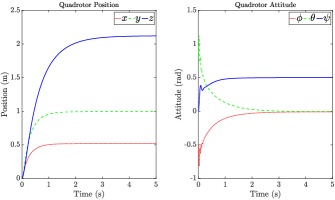
Figure 1: Simulation results for Quadrotor: (left) response of the position; (right) response of the attitude.

5 Conclusion

In this paper, a controller based on potential energy shaping for a quadrotor has been designed such that the upward equilibrium points have been stabilized. In contrast to previous works, the general complete solution of the matching equation has been derived utilizing the method of Pfaffian differential equation. The desired potential energy was designed such that using a simple change of coordinate, any upward position was reachable. Finally, the controller has been simulated and the results confirmed the theory.

References

• [1] B. Salamat, A. M. Tonello, A swash mass pendulum with passivity-based control, IEEE Robotics and Automation Letters 6 (2021) 199–206. doi:10.1109/LRA.2020.3037861.
• [2] B. Salamat, A. Yaghmaei, G. Elsbacher, A. M. Tonello, M. J. Yazdanpanah, An innovative control design procedure for under-actuated mechanical systems: Emphasizing potential energy shaping and structural preservation, IEEE Open Journal of Control Systems 2 (2023) 356–365. doi:10.1109/OJCSYS.2023.3320512.
• [3] A. Donaire, R. Mehra, R. Ortega, S. Satpute, J. G. Romero, F. Kazi, N. M. Singh, Shaping the energy of mechanical systems without solving partial differential equations, in: 2015 American Control Conference (ACC), 2015, pp. 1351–1356. doi:10.1109/ACC.2015.7170921.
• [4] B. Yüksel, C. Secchi, H. H. Bülthoff, A. Franchi, Aerial physical interaction via IDA-PBC, The International Journal of Robotics Research 38 (4) (2019) 403–421.
• [5] M. E. Guerrero, D. Mercado, R. Lozano, C. García, Passivity based control for a quadrotor uav transporting a cable-suspended payload with minimum swing (2015) 6718–6723.
• [6] C. Souza, G. Raffo, E. Castelan, Passivity based control of a quadrotor uav, IFAC Proceedings Volumes 47 (3) (2014) 3196–3201, 19th IFAC World Congress. doi:https://doi.org/10.3182/20140824-6-ZA-1003.02335.
• [7] J. Acosta, M. Sánchez, A. Ollero, Robust control of underactuated aerial manipulators via IDA-PBC, in: 53rd IEEE Conference on Decision and Control, 2014, pp. 673–678. doi:10.1109/CDC.2014.7039459.
• [8] B. Yüksel, C. Secchi, H. H. Bülthoff, A. Franchi, Reshaping the physical properties of a quadrotor through ida-pbc and its application to aerial physical interaction, in: 2014 IEEE International Conference on Robotics and Automation (ICRA), 2014, pp. 6258–6265. doi:10.1109/ICRA.2014.6907782.
• [9] R. Ortega, E. Garcia-Canseco, Interconnection and damping assignment passivity-based control: A survey, European Journal of control 10 (5) (2004) 432–450.
• [10] M. R. J. Harandi, H. D. Taghirad, Reformulation of matching equation in potential energy shaping, IEEE Transactions on Automatic Control.
• [11] M. R. J. Harandi, M. Namvar, H. D. Taghirad, Stabilization of robots with actuator constraints via interconnection and damping assignment, IEEE Transactions on Control Systems Technology.
• [12] M. E. Guerrero-Sánchez, D. A. Mercado-Ravell, R. Lozano, C. D. García-Beltrán, Swing-attenuation for a quadrotor transporting a cable-suspended payload, ISA transactions 68 (2017) 433–449.
• [13] M. E. Guerrero-Sanchez, H. Abaunza, P. Castillo, R. Lozano, C. Garcia-Beltran, A. Rodriguez-Palacios, Passivity-based control for a micro air vehicle using unit quaternions, Applied Sciences 7 (1). doi:10.3390/app7010013.
• [14] B. Yüksel, C. Secchi, H. H. Bülthoff, A. Franchi, Aerial physical interaction via ida-pbc, The International Journal of Robotics Research 38 (4) (2019) 403–421. doi:10.1177/0278364919835605.
• [15] M. R. J. Harandi, H. D. Taghirad, Solution of matching equations of IDA-PBC by pfaffian differential equations, International Journal of Control 95 (12) (2022) 3368–3378.