Many-body thermal states on a quantum computer: a variational approach.
Abstract
Many-body quantum states at thermal equilibrium are ubiquitous in nature. Investigating their dynamical properties is a formidable task due to the complexity of the Hilbert space they live in. Quantum computers may have the potential to effectively simulate quantum systems, provided that the many-body state under scrutiny can be faithfully prepared via an efficient algorithm. With this aim, we present a hybrid quantum–classical variational quantum algorithm for the preparation of the Gibbs state of the quantum model. Our algorithm is based on the Grover and Rudolph parametrized quantum circuit for the preparation of the Boltzmann weights of the Gibbs state, and on a parity-preserving ansatz for the allocation of the eigenenergy basis to their respective Boltzmann weight. We explicitly show, with a paradigmatic few-body case instance, how the symmetries of a many-body system can be exploited to significantly reduce the exponentially increasing number of variational parameters needed in the Grover and Rudolph algorithm. Finally, we show that the density matrix, of the Gibbs state of the model, obtained by statevector simulations for different parameters, exhibits a fidelity close to unity with the exact Gibbs state; this highlights the potential use of our protocol on current quantum computers.
1 Introduction
Quantum many-body systems present formidable challenges due to the inherent complexity of the Hilbert space they encompass Bengtsson2006 . Even the task of finding the ground-state of such systems is generally categorized as an NP-hard problem Barahona1982 . A recent and promising approach for tackling computational problems that are computationally demanding on classical computers is to harness the power of quantum computers Harrow2017 . However, it is important to note that the current state of quantum computation is constrained to the capabilities achievable on NISQ (Noisy Intermediate-Scale Quantum) computers Preskill2018quantumcomputingin . These machines are limited in that they can only apply quantum circuits of limited depth to a few noisy qubits before issues such as decoherence and gate errors compromise the accuracy of the obtained results.
In the past decade, a hybrid quantum–classical paradigm has been proposed as a means to harness the best of both classical and NISQ quantum computation Bharti2022 . These quantum–classical algorithms delegate the classically intractable part of an algorithm to the quantum computer, while performing efficiently subroutines on a classical computer, such as objective function optimization. A paradigmatic example of such procedures are variational quantum algorithms (VQAs) Cerezo2020 , where a parametrized quantum circuit (PQC), along with the classical optimizer, is tasked to prepare the quantum state encoding the solution to a given problem Tilly2022 . VQAs have been applied to a variety of quantum many-body problems, ranging from determining the electronic structure of small molecules Ratini2022 , investigating the onset of exotic phases of matter Consiglio2022 , to detecting entanglement Consiglio2022a .
At the same time, one of the main applications of quantum computing is expected to be the simulation of quantum many-body systems. In particular, simulating a quantum system at thermal equilibrium is key for several disciplines, including quantum chemistry, biology and combinatorial optimisation. Evidently, preparing a quantum many-body system at thermal equilibrium is QMA-hard Watrous2008 . Different quantum algorithms have been proposed for the preparation of thermal states based on fluctuation theorems Holmes2022 , imaginary time evolution Motta2020 , utilizing a generalized quantum assisted simulator Haug2022 and via adiabatic quantum computation Schaller2008 .
In this chapter we illustrate a thermal state preparation algorithm for a quantum many-body system based on the VQA first proposed in Ref. Consiglio2023a , where the PQC acts on an ancillary and a system register on which, respectively, the Boltzmann distribution and the Gibbs state are prepared. The advantage of this approach is that the von Neumann entropy, which is not an observable, can be determined without truncation. We apply our algorithm to the spin- Heisenberg Hamiltonian utilizing the Grover and Rudolph algorithm Grover2002 for preparing the Boltzmann distribution, highlighting how the symmetries of the model can be utilized to reduce the number of variational parameters in the circuit, followed by using a parity-preserving ansatz for diagonalizing the Hamiltonian. The chapter is organized as follows: in Sec. 2 we introduce the Hamiltonian of which we aim to prepare the thermal state; in Sec. 3 we present the Grover and Rudolph algorithm used to prepare probability distribution functions on a quantum computer; in Sec. 4 we implement the symmetries of the model in order to reduce the number of variational parameters used for the thermal state preparation; in Sec. 5 we present our VQA and its performance in preparing the thermal state; finally, in Sec. 6 we draw future prospects of our approach.
2 The model
In this Section we present the quantum many-body system of which we will prepare the thermal equilibrium state via a VQA. For the sake of completeness, we include a thorough derivation of its exact solution, which, due to the quadratic nature of the Hamiltonian in the fermionic representation, can be achieved both for finite and infinite system sizes.
Let us consider a 1D spin- system with periodic boundary conditions exhibiting nearest-neighbor interactions of Heisenberg type in the plane, subject to a uniform magnetic field in the transverse direction, see Fig. 1 for a finite-size instance. The spin- Hamiltonian LIEB1961407 is given by
| (1) |
where ( is the spin- operator sitting on site of a 1D lattice composed of even particles. The anisotropy parameter defines the model (), the Ising () and the model (), with the last two belonging to the same universality class. In the following, the diagonalization is carried out for arbitrary and .
[width=0.5]model_3.png
One can rewrite Eq. (1) in terms of Pauli matrices
| (2) |
and turn to the spin ladder operators , resulting in
| (3) |
where in the last steps and have been used. We have also set and rescaled the Hamiltonian by the constant term . Applying the Jordan-Wigner transformation:
| (4) |
the Hamiltonian in the fermionic representation reads
| (5) |
where h.c. denotes the hermitian conjugate and the last term on the RHS accounts for the periodic boundary conditions, by defining the Parity operator . The Parity operator has eigenvalues , denoting, respectively, the positive and the negative parity subspace. Hence, introducing the projectors on the positive and negative parity subspaces , Eq. (5) can be cast in a direct sum of disjoint subspaces
| (6) |
and
| (7) |
where antiperiodic boundary conditions, , hold for , and periodic boundary conditions, , hold for . While parity effects may become relevant for finite-size systems Damski2014 ; Franchini2016a , in the thermodynamic limit , they can be neglected being of order . In the following we will diagonalize Eq. (6) in the respective parity subspaces for finite size systems.
2.1 Positive parity subspace diagonalization
Because of the translational invariance of the system, we can perform a Fourier transformation of the fermionic operators,
| (8) |
where the momenta are chosen in order to satisfy the antiperiodic boundary conditions for , and , with integers. The factor has been introduced so as to end up with a real Hamiltonian, reading
| (9) |
The spinless, quadratic Hamiltonian in Eq. (9) is finally diagonalized via a Bogoliubov transformation
| (10) |
yielding
| (11) |
where the single-particle energy spectrum is given by
| (12) |
The ground-state of is given by the vacuum of the fermions and has energy
| (13) |
and the full spectrum of is derived by adding an even number of fermions to the ground-state
| (14) |
where is the subset of the power set of with an even number of terms.
2.2 Negative parity subspace diagonalization
The diagonalization of the model in the negative parity subspace follows closely that in the positive one and is sketched below. In order to fulfill the periodic boundary condition for the negative parity subspace Hamiltonian , the Fourier transformation is carried over with integers. The Fourier transformation of reads
| (15) |
where the 0-mode is occupied, whereas the -mode is empty in the ground-state of . Performing a Bogoliubov rotation as in the case of , we obtain that the ground-state energy of is given by
| (16) |
where
| (17) |
Similarly to , the full spectrum of is derived by adding an even number of fermions to the ground-state
| (18) |
where is the subset of the power set of with an even number of terms.
2.3 Gibbs density matrix
A system, with Hamiltonian , at thermal equilibrium with a bath at (inverse) temperature , where is the Boltzmann constant, is described by a density matrix , dubbed the Gibbs state: , where is the partition function.
Because of the direct sum structure of the Hamiltonian in Eq. (6), the thermal state of the spin system can also be cast in a direct sum form:
| (19) |
where are the eigenstates of and are the Boltzmann weights giving the probability distribution function (PDF) of the Gibbs distribution. The latter is composed by
| (20) |
From the non-interacting nature of the Hamiltonian and its set of symmetries, it is evident that there is a high degree of degeneracy in the Hamiltonian spectrum. In the following we will analytically determine how many distinct ’s appear in Eq. (20), in order to minimize the number of necessary variational parameters in the PQC, capable of reproducing the Boltzmann distribution, and hence the Gibbs state.
2.4 Degeneracies in the energy spectrum
Let us start identifying the number of distinct energy levels in the positive parity subspace. Because of the translational symmetry, the single-particle energy spectrum is invariant under momentum inversion , as evident from Eq. (12) being an even function of : .
Clearly, the state with zero fermions, i.e., the ground-state, is non-degenerate. The next set of energies we analyze is that with two fermions added to the ground-state, that is , where . The number of 2-fermions energy levels is given by the binomial of which energy levels are non-degenerate. This can be readily seen, as degenerate levels occur in the form
| (21) |
with . On the other hand, non-degenerate levels occur in the form
| (22) |
Hence, non-degenerate levels in the two-fermions excitation spectrum are given by how many distinct ’s can be selected in Eq. (22). This number is obtained by observing that the momenta are symmetric around 0, and hence the number of ways to chose one momentum out of momenta is trivially given by . Moreover, as Eqs. (21) give rise to the same energy, the degeneracy is always four-fold in this particle sector. To summarise, out of the energy levels, there are 4-fold degenerate energy levels, with the remaining being non-degenerate.
Moving to the 4-fermion excited states, one can proceed in a similar way by identifying, out of the 4-fermion excitation energy levels, as non-degenerate levels being those with energy
| (23) |
where . Hence, the non-degenerate levels of the 4-fermion excited states are , corresponding to the number of distinct sets that can be selected from the available momenta in the positive subset of . The degrees of degeneracy in the 4-particles sector are occurring, respectively, times.
Generalizing the above procedure to an arbitrary -fermion energy subspace, for a chain of length , one obtains that out of the -fermion excitation energy levels
-
•
the number of 1-fold degenerate levels is
-
•
the number of 4-fold degenerate levels is
-
•
the number of 16-fold degenerate levels is
-
•
the number of 64-fold degenerate levels is
-
•
the number of -fold degenerate levels is
Clearly, the maximum degree of degeneracy in the -fermion energy subspace is , with being a non-negative integer. The procedure just described determines the degree of degeneracy and the number of energy levels in each degenerate subspace of can be straightforwardly applied also to the negative parity subspace, which will not be reported here to avoid redundancy.
3 Preparing probability distributions on a quantum computer
In this Section we move to the main aim of this chapter: preparing a thermal state via a VQA. First we focus on preparing the Boltzmann distribution of the model entailed by Eq. (20).
Grover and Rudolph Grover2002 first described a procedure to prepare log-concave probability density functions on a quantum computer. However, this approach was later proven that it does not achieve a quantum speed-up in general Herbert2021 . Modern approaches resort to VQAs Nakaji2022 ; Dasgupta2022 ; Kumar2023 , whereby parametrized ansätze are used to prepare the probability distribution on a quantum register: by varying the parameters and minimizing a relevant cost function, such as the relative entropy. Similar, in this vein, is the generative adversarial network (GAN), where the classical optimizer is replaced by a classical neural network, acting as a discriminator for the probability distribution Zoufal2019 ; Situ2020 ; Agliardi2022 .
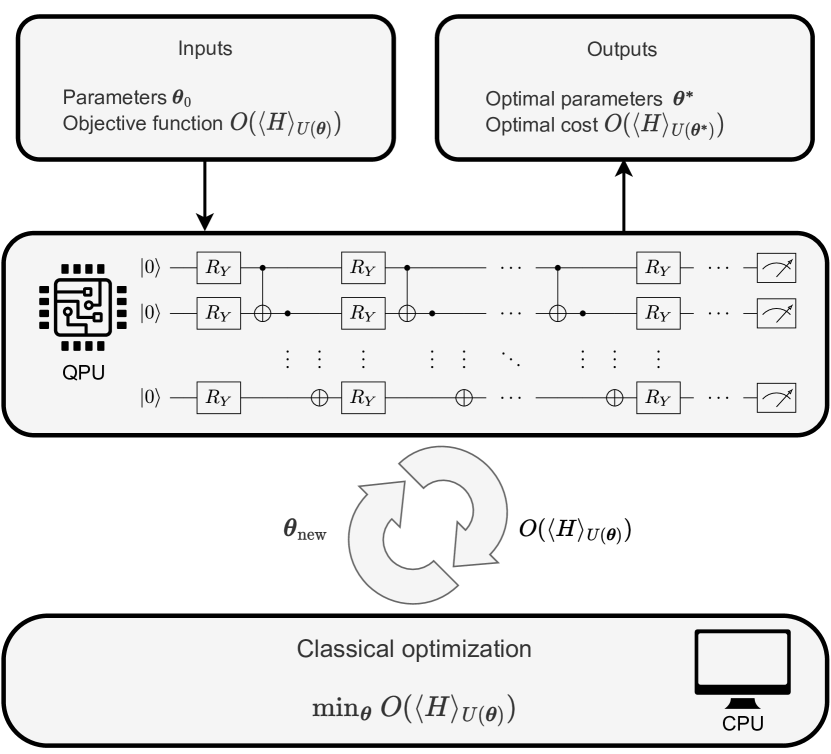
A VQA comprises several modular components that can be readily combined, extended, and improved with developments in quantum hardware and theory Bharti2022 . These components include: the objective function, the cost function to be variationally optimized; the PQC, composed of unitary gates that are updated in the optimization procedure; and the classical optimizer, the method used to obtain the optimal circuit parameters that optimize the objective function. Fig. 2 highlights the modules of a VQA.
To prepare the Boltzmann distribution of the model, we take the approach of utilizing a VQA, alongside a parametrized ansatz in the form of Grover and Rudolph Grover2002 . In this case, an -qubit ansatz requires parameters, and parameterized gates, most of which are multi-controlled. An gate acting on one qubit is given by
| (24) |
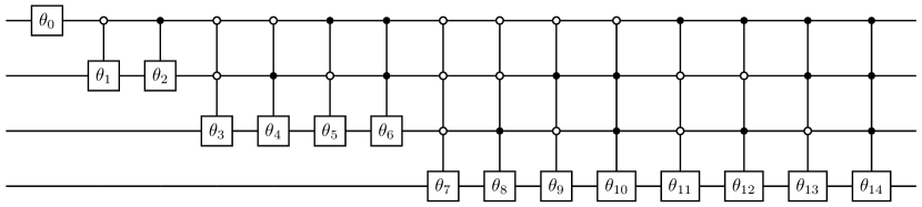
Controlled gates act on two or more qubits, where one or more qubits act as a control for some operation. The most common example is the CNOT gate, which performs the NOT operation on the second qubit only when the first qubit is the state , otherwise it leaves the state unchanged. In quantum circuit diagrams, a black dot represents the control qubit activating the controlled gate when in the state , while a white dot represents the control qubit activating the controlled gate when in the state . As a result, since the Grover and Rudolph algorithm serves to create a probability distribution from the entries of the first column, it utilizes only parametrized orthogonal (real unitary) gates. Note that an extended algorithm was proposed by Ref. Benenti2009 to obtain an optimal purification of an -qudit state.
Let us consider the case for , with Fig. 3 showing the circuit. Each box represents the gate with the relevant parameter, and the black and white dots represent the control qubits. For example, the gate with acts only on qubit 3 if qubit 0 is in the state , qubit 1 is in the state , and qubit 2 is in the state . Since there are possible binary controls for a -qubit controlled gate, one can see how the circuit scales exponentially, both in number of gates and number of parameters. Our goal in this manuscript is the reduce the number of parameters in the circuit shown in Fig. 3, by exploiting the symmetries of the model giving rise to the degeneracies in the energy levels obtained in Sec. 2.4.
The action of the circuit in Fig. 3 acting on the all-zero four-qubit state results in
| (25) |
The states and are the computational basis states of one qubit. As such, extending the computational basis states for qubits is simply done by computing the tensor product of all combinations of the states and up to qubits. For example, the computational basis states of two qubits are . As a result, when measuring the quantum state in Eq. (25) in the computational basis, we end up with the following probabilities for each configuration:
| (26a) | ||||
| (26b) | ||||
| (26c) | ||||
| (26d) | ||||
| (26e) | ||||
| (26f) | ||||
| (26g) | ||||
| (26h) | ||||
| (26i) | ||||
| (26j) | ||||
| (26k) | ||||
| (26l) | ||||
| (26m) | ||||
| (26n) | ||||
| (26o) | ||||
| (26p) | ||||
If one knows beforehand the discrete probability distribution, then, by taking specific ratios of expressions in Eqs. (26), one can relate the parameters to ratios of probabilities, e.g.,
| (27) |
By iterating this procedure for all , one can readily obtain
| (28) |
where ranges from , and from .
4 Few-body XY chain
To illustrate an instance of the Gibbs PDF preparation via the Grover and Rudolph algorithm where the degeneracies of the energy levels allow for a reduction of the number of variational parameters needed in the PQC, let us restrict to a few-body scenario. This allows to better keep track of the protocol relying on the analytic expressions of the eigenenergies. Let us focus on the chain.
Since the model is non-interacting, the spectrum is given by the single-particle energies, as discussed in Section 2. The model is also symmetric, when the eigenenergies are calculated with the modes ordered lexicographically, we can assign the first half of the computational basis states to cover , with the latter half to cover . The eigenenergies are:
| (29a) | ||||
| (29b) | ||||
| (29c) | ||||
| (29d) | ||||
| (29e) | ||||
| (29f) | ||||
| (29g) | ||||
| (29h) | ||||
We start to look at the Boltzmann coefficients generated by the eigenenergies in the negative parity sector. In the case of the
| (30) |
Next we find that
| (31) |
and
| (32) |
due to the pairs of degeneracies. Furthermore
| (33) |
Now looking at the Boltzmann coefficients given by the eigenenergies in the positive parity sector:
| (34) |
and
| (35) |
Moreover, while we cannot determine the exact value of and , due to their dependency on and , we can still relate them through
| (36) |
Finally, we also have that
| (37) |
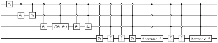
Thus we have managed to eliminate 8 parameters from a total of 15. This may be due to the fact that we have single-particle energy levels in both the positive and the negative parity subspace. However we also have the fact that in the negative parity subspace, the sum of the energies of the - and 0-modes sum always up to 2, hence giving an additional constraint. This result may hint towards the fact that for the model composed of particles, the number of parameters needed to characterize its Boltzmann distribution is . Fig. 4 represents the PQC in Fig. 3 with the reduced number of parameters obtained from Eqs. (30) - (37).
5 Structure of the VQA
We utilize the algorithm proposed in Ref. Consiglio2023a to prepare Gibbs states of the model. Suppose one chooses a Hamiltonian and inverse temperature . For a general state , one can define a generalized Helmholtz free energy as
| (38) |
where the von Neumann entropy can be expressed in terms of the eigenvalues, , of ,
| (39) |
Since the Gibbs state is the unique state that minimizes the free energy, a variational form can be put forward that takes Eq. (38) as an objective function, such that
| (40) |
In this case, is the probability of getting the eigenstate from the ensemble .
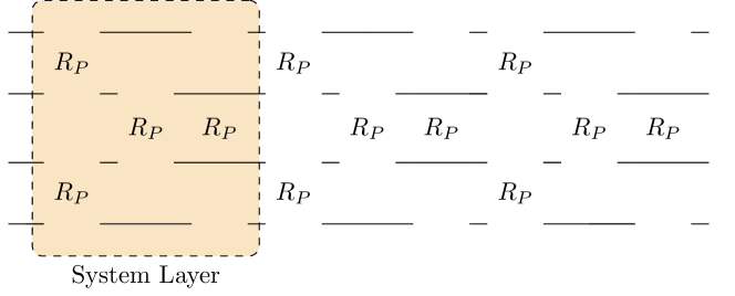
The PQC, as shown in Fig. 5, is composed of a unitary gate acting on the ancillary qubits, and a unitary gate acting on the system qubits, with CNOT gates in between. Note that the circuit notation we are using here means that there are qubits for both the system and the ancillae, as well as CNOT gates that act in parallel, . The parametrized unitary acting on the ancillae, followed by CNOT gates between the ancillary and system qubits, is responsible for preparing a probability distribution on the system. The parametrized unitary is then applied on the system qubits to transform the computational basis states into the eigenstates of the Hamiltonian.
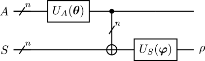
Throughout the paper we will describe unitary operations and density matrices in the computational basis. We will also denote the -fold tensor product of a state , of an -qubit register , as , where . Denote a general unitary gate of dimension , as . Starting with the initial state of the -qubit register, , we apply the unitary gate on the ancillae to get a quantum state , such that , where and is the identity acting on the system. Since is applied to the all-zero state in the ancillary register, then the operation serves to extract the first column of the unitary operator , as discussed in Section 3. The next step is to prepare a classical probability mixture on the system qubits, which can be done by applying CNOT gates between each ancilla and system qubit. This results in a state
| (41) |
By then tracing out the ancillary qubits, we arrive at
| (42) |
ending up with a diagonal mixed state on the system, with probabilities given directly by the absolute square of the entries of the first column of , that is, . If the system qubits were traced out instead, we would end up with the same diagonal mixed state,
| (43) |
This implies that by measuring in the computational basis of the ancillary qubits, we can determine the probabilities , which can then be post-processed to determine the von Neumann entropy of the state via Eq. (39) (since the entropy of is the same as that of ).
The unitary gate then serves to transform the computational basis states of the system qubits to the eigenstates of the Gibbs state, once it is optimized by the VQA, such that
| (44) |
where the expectation value of the Hamiltonian can be measured. Ideally, at the end of the optimization procedure, and , so that we get
| (45) |
Finally, we define the objective function of our VQA to minimize the free energy (38), via our constructed PQC, to obtain the Gibbs state
| (46) |
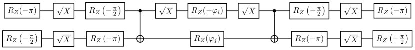
After optimization, the system register will (ideally) contain the prepared Gibbs state. In Refs. Consiglio2023a ; Consiglio2023b , is the ansatz responsible for preparing the Boltzmann distribution, while is the ansatz responsible for preparing the eigenstates of the Hamiltonian. In this work, we replace in Fig. 5 by the ansatz in Fig. 4, and optimize to obtain the Gibbs state of the model. is a parity-preserving ansatz, given by a brick-wall layering of gates, denoted as
| (51) |
As one can see from the unitary itself, any input state will have the same parity as the output state, and so, an ansatz constructed solely of parity-preserving gates will also be parity-preserving. The decomposed unitary gate is shown in Fig. 6, while the entire circuit of is shown in Fig. 7.
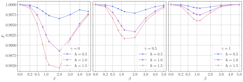
To assess the performance of the VQA, we utilize the Uhlmann-Josza fidelity as a figure of merit Uhlmann2011 , defined as . This fidelity measure quantifies the “closeness” between the prepared state and the target Gibbs state, making it a commonly-employed metric for distinguishability. Fig. 8 shows the fidelity of the prepared Gibbs state with the theoretical Gibbs state of the four-qubit model at and , across a broad range of temperatures. Three layers of both and were used for all simulations. Fig. 8 shows that the fidelity, while dipping at intermediary temperatures, still achieves values greater than 98% for all models and temperatures. Interestingly, the results for appear to be slightly less optimal. This may due to the fact that the model belongs to a different universality class than the and Ising model, exhibiting an additional symmetry, the conservation of the total magnetization.
6 Conclusion
In this chapter we have addressed the problem of preparing a quantum many-body thermal state via a variational quantum algorithm suitable for NISQ computers. We utilized a parametrized quantum circuit composed of two blocks: the former acting on an ancillary register tasked with reproducing the Boltzmann distribution, with the latter acting on the system register tasked with rotating the system’s state from the computational basis to the eigenenergy basis. The two registers are connected by a set of CNOT gates, and the optimizer is tasked with minimizing the generalized Helmholtz energy in order to prepare the Gibbs state on the system register.
We have improved on the Grover and Rudolph procedure for the preparation of an arbitrary probability distribution function, by reducing the number of exponential parameters needed in the VQA exploiting the symmetries of the spin- Heisenberg model. We have then applied our protocol to a four-site chain and showed that our VQA is able to reach almost unit fidelity in statevector simulations by combining the Grover and Rudolph algorithm, with a reduced number of variational parameters acting on the ancillary register, and a parity-preserving ansatz on the system register. Although we have applied our protocol to small system sizes, our results hint toward the fact that a sub-exponential number of variational parameters are necessary for the preparation of a many-body Gibbs distribution by exploiting the degeneracies in the energy spectrum.
Acnowledgements
The Authors acknowledge discussions with Francesco Plasina and Jacopo Settino on the topic of this chapter. TJGA ackowledges funding through the IPAS+ (Internationalisation Partnership Awards Scheme +) QIM project by the MCST (The Malta Council for Science & Technology). M.C. acknowledges funding by TESS (Tertiary Education Scholarships Scheme).
References
- [1] Ingemar Bengtsson and Karol Zyczkowski. Geometry of Quantum States: An Introduction to Quantum Entanglement. Cambridge University Press, 2006.
- [2] F. Barahona. On the computational complexity of Ising spin glass models. Journal of Physics A: Mathematical and General, 15(10):3241–3253, oct 1982.
- [3] Aram W. Harrow and Ashley Montanaro. Quantum computational supremacy. Nature, 549(7671):203–209, sep 2017.
- [4] John Preskill. Quantum Computing in the NISQ era and beyond. Quantum, 2:79, August 2018.
- [5] Kishor Bharti, Alba Cervera-Lierta, Thi Ha Kyaw, Tobias Haug, Sumner Alperin-Lea, Abhinav Anand, Matthias Degroote, Hermanni Heimonen, Jakob S. Kottmann, Tim Menke, Wai-Keong Mok, Sukin Sim, Leong-Chuan Kwek, and Alán Aspuru-Guzik. Noisy intermediate-scale quantum algorithms. Rev. Mod. Phys., 94:015004, Feb 2022.
- [6] M. Cerezo, Andrew Arrasmith, Ryan Babbush, Simon C. Benjamin, Suguru Endo, Keisuke Fujii, Jarrod R. McClean, Kosuke Mitarai, Xiao Yuan, Lukasz Cincio, and Patrick J. Coles. Variational quantum algorithms. Nature Reviews Physics, 3(9):625–644, aug 2021.
- [7] Jules Tilly, Hongxiang Chen, Shuxiang Cao, Dario Picozzi, Kanav Setia, Ying Li, Edward Grant, Leonard Wossnig, Ivan Rungger, George H. Booth, and Jonathan Tennyson. The Variational Quantum Eigensolver: A review of methods and best practices. Physics Reports, 986:1–128, nov 2022.
- [8] Leonardo Ratini, Chiara Capecci, Francesco Benfenati, and Leonardo Guidoni. Wave Function Adapted Hamiltonians for Quantum Computing. Journal of Chemical Theory and Computation, 18(2):899–909, feb 2022.
- [9] Mirko Consiglio, Wayne J Chetcuti, Carlos Bravo-Prieto, Sergi Ramos-Calderer, Anna Minguzzi, José I Latorre, Luigi Amico, and Tony J G Apollaro. Variational quantum eigensolver for SU(N) fermions. Journal of Physics A: Mathematical and Theoretical, 55(26):265301, jul 2022.
- [10] Mirko Consiglio, Tony J G Apollaro, and Marcin Wieśniak. Variational approach to the quantum separability problem. Physical Review A, 106(6):062413, dec 2022.
- [11] John Watrous. Quantum Computational Complexity, 2008.
- [12] Zoe Holmes, Gopikrishnan Muraleedharan, Rolando D. Somma, Yigit Subasi, and Burak Şahinoğlu. Quantum algorithms from fluctuation theorems: Thermal-state preparation. Quantum, 6:825, October 2022.
- [13] Mario Motta, Chong Sun, Adrian T. K. Tan, Matthew J. O’Rourke, Erika Ye, Austin J. Minnich, Fernando G. S. L. Brandão, and Garnet Kin-Lic Chan. Determining eigenstates and thermal states on a quantum computer using quantum imaginary time evolution. Nature Physics, 16(2):205–210, Feb 2020.
- [14] Tobias Haug and Kishor Bharti. Generalized quantum assisted simulator. Quantum Science and Technology, 7(4):045019, aug 2022.
- [15] Gernot Schaller. Adiabatic preparation without quantum phase transitions. Physical Review A, 78(3):032328, sep 2008.
- [16] Mirko Consiglio, Jacopo Settino, Andrea Giordano, Carlo Mastroianni, Francesco Plastina, Salvatore Lorenzo, Sabrina Maniscalco, John Goold, and Tony J. G. Apollaro. Variational gibbs state preparation on nisq devices, 2023.
- [17] Lov Grover and Terry Rudolph. Creating superpositions that correspond to efficiently integrable probability distributions, 2002.
- [18] Elliott Lieb, Theodore Schultz, and Daniel Mattis. Two soluble models of an antiferromagnetic chain. Annals of Physics, 16(3):407–466, 1961.
- [19] Bogdan Damski and Marek M Rams. Exact results for fidelity susceptibility of the quantum Ising model: the interplay between parity, system size, and magnetic field. Journal of Physics A: Mathematical and Theoretical, 47(2):025303, jan 2014.
- [20] Fabio Franchini. An Introduction to Integrable Techniques for One-Dimensional Quantum Systems, volume 940 of Lecture Notes in Physics. Springer International Publishing, Cham, sep 2017.
- [21] Steven Herbert. No quantum speedup with grover-rudolph state preparation for quantum monte carlo integration. Phys. Rev. E, 103:063302, Jun 2021.
- [22] Kouhei Nakaji, Shumpei Uno, Yohichi Suzuki, Rudy Raymond, Tamiya Onodera, Tomoki Tanaka, Hiroyuki Tezuka, Naoki Mitsuda, and Naoki Yamamoto. Approximate amplitude encoding in shallow parameterized quantum circuits and its application to financial market indicators. Phys. Rev. Res., 4:023136, May 2022.
- [23] Kalyan Dasgupta and Binoy Paine. Loading probability distributions in a quantum circuit, 2022.
- [24] Rohit Taeja Kumar and Ankur Raina. Generating probability distributions using variational quantum circuits, 2023.
- [25] Christa Zoufal, Aurélien Lucchi, and Stefan Woerner. Quantum generative adversarial networks for learning and loading random distributions. npj Quantum Information, 5(1):103, Nov 2019.
- [26] Haozhen Situ, Zhimin He, Yuyi Wang, Lvzhou Li, and Shenggen Zheng. Quantum generative adversarial network for generating discrete distribution. Information Sciences, 538:193–208, 2020.
- [27] Gabriele Agliardi and Enrico Prati. Optimal tuning of quantum generative adversarial networks for multivariate distribution loading. Quantum Reports, 4(1):75–105, 2022.
- [28] Giuliano Benenti and Giuliano Strini. Optimal purification of a generic -qudit state. Phys. Rev. A, 79:052301, May 2009.
- [29] Mirko Consiglio. Variational quantum algorithms for gibbs state preparation, 2023.
- [30] Armin Uhlmann. Transition Probability (Fidelity) and Its Relatives. Foundations of Physics, 41(3):288–298, 2011.