Generalized Zeno effect and entanglement dynamics induced by fermion counting

Abstract

We study a one-dimensional lattice system of free fermions subjected to a generalized measurement process: the system exchanges particles with its environment, but each fermion leaving or entering the system is counted. In contrast to the freezing of dynamics due to frequent measurements of lattice-site occupation numbers, a high rate of fermion counts induces fast fluctuations in the state of the system. Still, through numerical simulations of quantum trajectories and an analytical approach based on replica Keldysh field theory, we find that instantaneous correlations and entanglement properties of free fermions subjected to fermion counting and local occupation measurements are strikingly similar. We explain this similarity through a generalized Zeno effect induced by fermion counting and a universal long-wavelength description in terms of an $\mathrm{SU}(R)$ nonlinear sigma model. Further, for both types of measurement processes, we present strong evidence against the existence of a critical phase with logarithmic entanglement and conformal invariance at finite measurement rates. Instead, we identify a well-defined and finite critical range of length scales on which signatures of conformal invariance are observable. While area-law entanglement is established beyond a scale that is exponentially large in the measurement rate, the upper boundary of the critical range is only algebraically large and thus numerically accessible.

I Introduction

Frequent projective measurements induce the quantum Zeno effect, the freezing of the evolution of a quantum system in an eigenstate of the measured observable [1]. For measurements of local observables in a spatially extended many-body system, these eigenstates exhibit area-law scaling of the entanglement entropy. The quantum Zeno effect, thus, stabilizes area-law entanglement even in systems that would in the absence of measurements unitarily evolve toward volume-law entanglement. Reducing the rate at which measurements are performed can lead to a novel type of dynamical phase transition between area-law and volume-law scaling of the entanglement entropy. Such measurement-induced phase transitions have first been described in quantum circuits [2, 3, 4, 5, 6, 7, 8, 9, 10, 11, 12, 13, 14, 15, 16, 17], and later also in dynamics generated by a time-independent Hamiltonian, including in fermionic [18, 19, 20, 21, 22, 23, 24, 25, 26, 27, 28, 29, 30, 31, 32, 33, 34, 35, 36, 37, 38, 39, 40], bosonic [41, 42, 43, 44, 45], and spin systems [46, 47, 48, 49, 50, 51]. Experimental studies of measurement-induced phase transitions have been performed with trapped ions [52, 53] and superconducting qubits [54, 55, 56]. But while the freezing of dynamics provides an intuitive explanation for area-law entanglement through repeated measurements, is it also a requirement? As we detail in the following, this question is of fundamental relevance for systems that are subjected to generalized measurements.

A generalized measurement is described by a collection of measurement operators $\hat{M}_{n}$ that obey the completeness relation $\sum_{n}\hat{M}_{n}^{\dagger}\hat{M}_{n}^{\vphantom{\dagger}}=1$, where the sum is over possible measurement outcomes labeled by the index $n$ [57]. If the state of a quantum system immediately before a generalized measurement performed at time $t$ is $\lvert\psi(t-0)\rangle$, then the outcome $n$ occurs with probability $p_{n}(t)=\left\langle\psi(t-0)\middle|\hat{M}_{n}^{\dagger}\hat{M}_{n}^{\vphantom{\dagger}}\middle|\psi(t-0)\right\rangle$, and the state of the system after the measurement is

$$\lvert\psi(t+0)\rangle=\frac{1}{\sqrt{p_{n}(t)}}\hat{M}_{n}\lvert\psi(t-0)\rangle.$$ (1)

Crucially, the measurement operators $\hat{M}_{n}$ need not be projectors. If they are not, performing a generalized measurement immediately after a measurement with outcome $n$ does generally not yield the same result $n$, and repeated generalized measurements do not lead to a freezing of the dynamics.

Here, we describe a novel mechanism that stabilizes area-law entanglement through repeated measurements but does not require the freezing of the dynamics associated with the conventional Zeno effect. We consider a one-dimensional lattice model of free fermions subjected to fermion counting. That is, each lattice is coupled to reservoirs, acting as drain and source of particles. The occupation of the reservoirs is monitored continuously, such that each fermion that leaves or enters the system is registered. This form of monitored loss and gain or fermion counting can be formulated as a continuous generalized measurement, where each measurement operator removes or adds a fermion at a particular lattice site. Therefore, a high rate of fermion counts causes the state of the system to fluctuate rapidly. At the same time, the local removal and addition of particles efficiently disentangles the many-body wave function, similarly to generalized [19] or projective [58] measurements of local occupation numbers, which conserve the total number of particles in the system, and induce a Zeno effect in the frequent-measurement limit.

To obtain a comprehensive understanding of the similarities and differences between these scenarios, we perform a comparative study of fermion counting and generalized measurements of local occupation numbers. Despite their starkly different dynamics, both models exhibit almost identical steady-state correlations and entanglement properties. We trace this striking similarity back to a generalized Zeno effect induced by fermion counting. The key feature the conventional and generalized Zeno effects have in common is the suppression of coherent dynamics, leading in turn to a suppression of the growth of entanglement.

More formally, we explain the near indistinguishability of the models with fermion counting and occupation measurements in terms of their correlations and entanglement properties through a common long-wavelength effective field theory, given by an $\mathrm{SU}(R)$ nonlinear sigma model (NLSM), derived in the framework of replica Keldysh field theory [36, 16, 58, 34]. The predictions from this analytical description are in agreement with our numerical results and provide strong evidence that both types of measurements lead to area-law entanglement for any nonzero measurement rate $\gamma$.

Recent studies have led to contradictory results concerning the existence of a measurement-induced entanglement transition in one-dimensional free fermions with conserved number of particles. Entanglement dynamics under continuous measurements of occupation numbers, described by either quantum state diffusion [59] or quantum jump trajectories [60] as considered in this work, have been studied in Ref. [19]. For both types of dynamics, there is numerical evidence for a measurement-induced Kosterlitz-Thouless (KT) transition at a finite critical measurement rate $\gamma_{c}$, separating a critical phase with logarithmic growth of the entanglement entropy as characteristic for a one-dimensional conformal field theory (CFT) [82] from an area-law phase. These findings suggest that the precise way in which measurements are implemented might affect nonuniversal properties such as the value of the critical measurement rate, but not whether there is a transition or not. Therefore, one is led to assume that this question is decided by the emergent long-wavelength behavior, which is expected to be universal in the sense that it is determined solely by spatial dimensionality and symmetries. In turn, symmetries are reflected in conservation laws, and both in quantum state diffusion and quantum jump trajectories, the number of particles is the only conserved quantity. The existence of a measurement-induced phase transition in one-dimensional free fermions with particle number conservation is corroborated by replica Keldysh theory for Dirac fermions with a linear dispersion relation [23].

However, based on the above assumption of universality, we should compare the results of Refs. [19, 23] to the findings of Ref. [58], which has studied free fermions under random projective measurements of occupation numbers, with analytical and numerical results indicating that there is no measurement-induced phase transition. Instead, for any finite measurement rate $\gamma$, the logarithmic growth of the entanglement entropy transitions into area-law behavior above an exponentially large scale $\ln(l_{*})\sim\gamma^{-1}$. For small values of the measurement rate, for which the theory is expected to become quantitatively accurate, this scale is beyond numerically accessible system sizes.

Here, we show analytically and numerically that clear signatures of the crossover to area-law entanglement can be observed on much smaller scales, well within the reach of finite-size numerics. Approximately logarithmic growth of the entanglement entropy is restricted to a critical range of length scales, bounded from below by $l_{0}\sim\gamma^{-1}$ and from above by $l_{c}\sim\gamma^{-2}$. Only within this critical range, we observe clear signatures of conformal invariance [19]. These results apply both to fermion counting and to generalized measurements of local occupation numbers. Therefore, our work further clarifies the impact of particle number conservation on measurement-induced dynamics of one-dimensional free fermionic systems: while there can be an entanglement transition if particle-number conservation is broken by the Hamiltonian that generates the unitary dynamics as in the Majorana model of Ref. [36], our results indicate that there is no transition if the Hamiltonian does conserve the number of particles, irrespective of whether the measurement operators are particle-number conserving.

This paper is organized as follows. In Sec. II, we summarize our key results. The models we study are introduced in Sec. III. Then, in Sec. IV, we describe signatures of the conventional and generalized Zeno effects for occupation measurements and fermion counting, respectively. An analytical description of our models in terms of a replica Keldysh field theory is introduced in Sec. V. We analyze the Gaussian field theory that applies in the weak-measurement limit in Sec. VI, and discuss the effect of fluctuations beyond the Gaussian theory in Sec. VII. A detailed comparison between our analytical predictions and numerical results is provided in Sec. VIII, where we consider spatial correlations, measures of entanglement, and signatures of conformal invariance in the steady state. Section IX contains our conclusions and an outlook on future research questions. Details of our analytical and numerical studies are described in several appendices.

II Key results

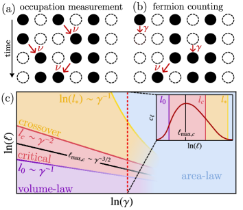
Figure 1: (a) Zeno effect for fermions on a one-dimensional lattice subjected to measurements of local occupation numbers. Frequent measurements freeze the system in classical configurations with each lattice site either occupied or empty (filled and empty circles). Incoherent hopping occurs at the slow rate $\nu=J^{2}/\gamma$. (b) Generalized Zeno effect induced by fermion counting. A high rate $\gamma$ of fermion counts corresponds to fast transitions between classical configurations. As in the conventional Zeno effect, additional slow processes occur at the rate $\nu$. (c) Schematic finite-size phase diagram for fermion counting and occupation measurements. For low measurement rates, the entanglement exhibits volume-law scaling below $l_{0}\sim\gamma^{-1}$ and grows logarithmically in the critical range between $l_{0}$ and $l_{c}\sim\gamma^{-2}$, before it slowly crosses over to area-low scaling, which is established beyond the exponentially large scale $\ln(l_{*})\sim\gamma^{-1}$. Inset: the effective central charge $c_{\ell}$ has a maximum at $\ell_{\mathrm{max},c}\sim\gamma^{-3/2}$.

Through analytical and numerical studies of free fermions on a one-dimensional lattice and subjected to fermion counting or generalized measurements of local lattice-site occupation numbers, we have obtained the following results:

Frequent particle loss and gain suppress coherent dynamics and stabilize area-law entanglement via a generalized Zeno effect.

Before we explain the generalized Zeno effect, let us briefly recall the conventional Zeno effect for a single particle on a one-dimensional lattice, subjected to repeated generalized measurements of lattice-site occupation numbers, $\hat{M}_{l}=\hat{n}_{l}$. The first measurement collapses the initial wave function $\lvert\psi\rangle$ of the particle to a state $\lvert l_{0}\rangle$ that is localized on a single lattice site $l_{0}$, chosen from $l\in\{1,\dotsc,L\}$ according to Born’s rule with probability $p_{l}=\left\langle\psi|\hat{n}_{l}|\psi\right\rangle$. Subsequent measurements, performed at a rate $\gamma$, yield the same result $l_{0}$, since the probability distribution after the first collapse is $p_{l}=\delta_{l,l_{0}}$. Coherent hopping with amplitude $J\ll\gamma$ can induce transitions $\lvert l_{0}\rangle\to\lvert l_{0}\pm 1\rangle$. However, these processes occur at second order in perturbation theory, that is, with a small rate $\nu=J^{2}/\gamma$. This suppression of coherent dynamics through frequent measurements is the essence of the conventional Zeno effect. The resultant slow dynamics are illustrated for a many-body system in Fig. 1(a).

To illustrate the generalized Zeno effect, we first consider a single fermionic lattice site with annihilation and creation operators $\hat{\psi}$ and $\hat{\psi}^{\dagger}$, respectively. Fermion counting is described by generalized measurements performed at a rate $\gamma$ and with measurement operators $\hat{M}_{-}=\hat{\psi}$ and $\hat{M}_{+}=\hat{\psi}^{\dagger}$. The completeness relation $\hat{M}_{-}^{\dagger}\hat{M}_{-}+\hat{M}_{+}^{\dagger}\hat{M}_{+}=1$ follows from canonical anticommutation relations. Repeated measurements cause the occupation of the lattice site to fluctuate between 0 and 1, realizing a random telegraph process [61]. The autocorrelation function of the occupation number $\hat{n}=\hat{\psi}^{\dagger}\hat{\psi}$ decays exponentially with a rate $\sim\gamma$. That is, the dynamics become faster for increasing measurement rate $\gamma$—the exact opposite of the freezing of the dynamics in the conventional Zeno effect.

In an extended lattice system with monitored loss and gain on each lattice site, the dynamics induced by measurements allow the system to ergodically explore all classical configurations of $N\in\{0,\dotsc,L\}$ particles distributed on $L$ lattice sites. Coherent hopping enables additional transitions between these configurations. Crucially, in analogy to the conventional Zeno effect, these transitions are suppressed for $J\ll\gamma$ and occur with a slow rate $\nu=J^{2}/\gamma$. Therefore, we refer to this phenomenon, which is illustrated in Fig. 1(b), as a generalized Zeno effect. The fact that coherent dynamics are suppressed by frequent fermion counts and that the classical configurations which dominate the dynamics for $J\ll\gamma$ have vanishing entanglement entropy rationalizes that fermion counting stabilizes area-law entanglement.

The generalized and conventional Zeno effects induce almost identical correlations and entanglement properties.

Even though the dynamics are strikingly different for fermion counting and occupation measurements, both lead to equivalent behavior in various measures of correlations and entanglement in the steady state. This includes density-density correlations, the entanglement entropy, and the bipartite mutual information. We observe a qualitative difference only in higher-order correlations as quantified through the tripartite mutual information, indicating that the tripartite mutual information probes properties that are not captured by the long-wavelength effective field theory, which is the same for both models as described next.

The similarity of correlations and entanglement properties can be explained in terms of a universal long-wavelength effective field theory.

Starting from a microscopic model of a fermionic lattice system, with each site coherently coupled to particle reservoirs acting as drain and source, a natural description of the dynamics of the system alone can be given in terms of a stochastic Schrödinger equation [60]. The stochastic Schrödinger equation describes the evolution of the state $\lvert\psi(t)\rangle$ of the system conditioned on the counting of fermions that are transferred between the system and reservoirs. As we show, the same quantum trajectories $\lvert\psi(t)\rangle$ are obtained from a description of fermion counting as generalized measurements that are performed at random times and with outcomes determined by Born’s rule. This equivalence enables an analytical description of the system dynamics in terms of a replica Keldysh field theory [36, 16, 58, 34], which we adopt to the case of generalized measurements. The field theory approach gives access to two types of observables: (i) Observables that are linear in the projector on the conditional state $\hat{\rho}(t)=\lvert\psi(t)\rangle\langle\psi(t)\rvert$, such as expectation values $\overline{\left\langle\hat{A}(t)\right\rangle}$ or temporal correlation functions $\overline{\left\langle\hat{A}(t)\hat{B}(t^{\prime})\right\rangle}$, where the overbar denotes the average over trajectories; and (ii) instantaneous observables that are nonlinear in $\hat{\rho}(t)$, such as connected equal-time correlation functions $\overline{\left\langle\hat{A}(t)\hat{B}(t)\right\rangle-\left\langle\hat{A}(t)\right\rangle\left\langle\hat{B}(t)\right\rangle}$ or the entanglement entropy. Observables of type (i) are encoded in the replica-symmetric sector of the theory, and observables of type (ii) in the replica-asymmetric or replicon sector. Fermion counting leads to exponential decay of the density autocorrelation function, which is an observable of type (i). In contrast, particle number conservation in the model with occupation measurements leads to diffusive decay. Formally, this difference between exponential and algebraic decay is reflected in the replica-symmetric sector being massive and massless for fermion counting and occupation measurements, respectively. However, in the long-wavelength limit, the replicon sector is in both cases described by the same massless effective field theory, given by an $\mathrm{SU}(R)$ NLSM. This common long-wavelength effective field theory description analytically explains the numerically observed equivalence of correlations and entanglement properties. Further, the theory predicts that there is no measurement-induced entanglement transition in these models. Instead, area-law entanglement is established for any nonzero measurement rate.

Breaking of particle number conservation through generalized measurements does not induce an entanglement transition.

Our model of fermion counting features particle-number-conserving unitary dynamics and generalized measurements that do not conserve the number of particles. In this regard, our work closes the gap between models that have previously been discussed in the literature: on the one hand, fully particle-number-conserving models of random generalized [19] or projective measurements [58]. These models do not exhibit an entanglement transition upon tuning the measurement rate. And on the other hand, the Majorana model of Ref. [36], in which particle number conservation is broken by the Hamiltonian that generates the unitary dynamics and, depending on the choice of parameters, also the measurement operators. This model does exhibit an entanglement transition. We find the long-wavelength effective replicon field theory to be identical for fermion counting as well as generalized and projective measurements of occupation numbers [58], but different for the Majorana model [36]. Therefore, the breaking of particle number conservation through measurements alone is insufficient to induce an entanglement transition.

Logarithmic growth of the entanglement entropy and signatures of conformal invariance are observable within a well-defined and finite critical range of length scales.

The renormalization-group (RG) flow of the NLSM indicates that area-law entanglement is established beyond a scale $l_{*}$ that is exponentially large in $\gamma^{-1}$. However, the RG-corrected Gaussian field theory predicts that for small measurement rates $\gamma$, properties that are characteristic for a critical phase, including logarithmic growth of the entanglement entropy and signatures of conformal invariance [19], can be observed within a finite critical range of length scales between $l_{0}\sim\gamma^{-1}$ and $l_{c}\sim\gamma^{-2}$ as illustrated in Fig. 1(c). Beyond $l_{c}$, there is a wide crossover region that separates the critical range from the onset of area-law scaling. Since $l_{c}$ is only algebraically large in $\gamma$, this scale is numerically accessible also for relatively small values of the measurement rate—even if area-law scaling beyond $l_{*}$ is not observable.

To precisely characterize the behavior of the entanglement entropy, we introduce a scale-dependent effective central charge $c_{\ell}$ for a subsystem of size $\ell$. On short scales $\ell\lesssim l_{0}\sim\gamma^{-1}$, the effective central charge $c_{\ell}$ grows with $\ell$, indicating volume-law scaling of the entanglement entropy; on an intermediate scale $\ell=\ell_{\mathrm{max},c}\sim\gamma^{-3/2}$, the central charge exhibits a maximum and thus becomes stationary, leading to logarithmic growth of the entanglement entropy; and on large scales $\ell\gtrsim l_{c}\sim\gamma^{-2}$, the central charge decreases; $c_{\ell}$ is expected to vanish, corresponding to area-law entanglement, beyond the exponentially large scale $l_{*}$. The numerically observed behavior of the effective central charge, illustrated schematically in Fig. 1(c), is in good agreement with our analytical predictions.

Evidence for emergent conformal invariance is provided by the collapse of the mutual information as a function of the cross ratio with the form predicted by conformal field theory [62, 19]. We perform a systematic numerical analysis of the mutual information for varying subsystem sizes, which reveals that this collapse occurs only for subsystem sizes within the critical range, corroborating that conformal invariance is violated at both short and large scales.

The results described above apply equally to fermion counting and occupation measurements. Differences between the two types of generalized measurements and deviations from conformal invariance even within the critical range can be seen in the tripartite mutual information.

Our detailed analytical and numerical analysis of the crossover from the critical to the area-law phase corroborates and refines the conclusion of Ref. [58], that the evidence for an entanglement transition of free fermions presented in Ref. [19] describes, in fact, a finite-size crossover phenomenon.

III Models

We consider two models of noninteracting fermions on a one-dimensional lattice undergoing unitary time evolution interspersed with generalized measurements. In both models, the unitary dynamics are generated by the Hamiltonian

$$\hat{H}=-J\sum_{l=1}^{L}\left(\hat{\psi}_{l}^{\dagger}\hat{\psi}_{l+1}^{\vphantom{\dagger}}+\hat{\psi}_{l+1}^{\dagger}\hat{\psi}_{l}^{\vphantom{\dagger}}\right),$$ (2)

where $\hat{\psi}_{l}$ and $\hat{\psi}_{l}^{\dagger}$ are fermionic annihilation and creation operators, respectively, on lattice sites $l\in\{1,\dotsc,L\}$ with periodic boundary conditions, $\hat{\psi}_{L+1}=\hat{\psi}_{1}$. The two models differ by the type of measurement process: in the first model, we consider monitored loss and gain of fermions on each lattice site; in the second model, we consider measurements of local occupation numbers, $\hat{n}_{l}^{\vphantom{\dagger}}=\hat{\psi}_{l}^{\dagger}\hat{\psi}_{l}^{\vphantom{\dagger}}$. Our main focus lies on the first model, with the second serving as a case of reference. Entanglement dynamics under continuous and random measurements of local occupation numbers have been studied in Refs. [18, 19], and under projective random measurements in Ref. [58].

In the following, we present two equivalent ways to describe quantum trajectories, that is, the evolution of the state vector of the fermionic many-body system, conditioned on a sequence of measurement outcomes. The first description in terms of a stochastic Schrödinger equation results naturally from microscopic physical models, for example, for the implementation of monitored loss and gain by coupling the system of interest to reservoirs, which are then subjected to continuous projective measurements [60]. In the more formal second description, generalized measurements are performed directly on the system at an externally imposed constant rate. This description has the technical advantage of lending itself naturally toward a reformulation as a replica Keldysh field theory, generalizing the construction of Ref. [58] for projective measurements. Crucially, the statistics of measurement times and outcomes, and the resulting quantum trajectory dynamics, are identical in both descriptions.

III.1 Stochastic Schrödinger equation

A minimal physical model for fermion counting consists of a quantum dot, that is, a single fermionic lattice site, tunnel-coupled to two fermionic reservoirs, which we assume to be in thermodynamic equilibrium at a low temperature. The chemical potentials of the reservoirs are chosen such that fermions can tunnel from the quantum dot to the first reservoir, the drain, and from the second reservoir, the source, to the quantum dot, but the reverse processes are inhibited. We obtain a theoretical description of fermion counting by integrating the Schrödinger equation for the quantum dot and reservoirs in discrete time steps $\Delta t$ using the Born and Markov approximations, that is, treating the coupling to the reservoirs perturbatively and assuming the reservoirs to have short correlation times as detailed in Appendix A. At each time step, the occupations of drain and source are measured projectively. These measurements indirectly count the number of fermions leaving or entering the quantum dot: finding modes of the drain and source to be occupied and empty, respectively, indicates that a fermion must have left or entered the quantum dot. A description of the dynamics of the quantum dot alone can be obtained by modeling the sequence of measurement results through appropriate stochastic processes. In the continuous time limit $\Delta t\to\mathrm{d}t$ and generalizing the setup to $L$ fermionic lattice sites, each in contact with its own drain and source, we obtain a stochastic Schrödinger equation for the state $\lvert\psi(t)\rangle$ of the fermionic lattice system,

$$\mathrm{d}\lvert\psi(t)\rangle=\left(\left\{-\mathrm{i}\hat{H}-\sum_{\alpha=\pm}\sum_{l=1}^{L}\left[\hat{L}_{\alpha,l}^{\dagger}\hat{L}_{\alpha,l}^{\vphantom{\dagger}}-\tilde{p}_{\alpha,l}(t)\right]\right\}\mathrm{d}t\right.\\ \left.+\sum_{\alpha=\pm}\sum_{l=1}^{L}\left[\frac{\hat{L}_{\alpha,l}}{\sqrt{\tilde{p}_{\alpha,l}(t)}}-1\right]\mathrm{d}N_{\alpha,l}(t)\right)\lvert\psi(t)\rangle.$$ (3)

The first line describes deterministic dynamics, governed by the Hamiltonian $\hat{H}$ in Eq. (2) and the jump operators

$$\hat{L}_{-,l}^{\vphantom{\dagger}}=\sqrt{\gamma_{-}/2}\,\hat{\psi}_{l}^{\vphantom{\dagger}},\qquad\hat{L}_{+,l}^{\vphantom{\dagger}}=\sqrt{\gamma_{+}/2}\,\hat{\psi}_{l}^{\dagger},$$ (4)

where the loss and gain rates $\gamma_{-}$ and $\gamma_{+}$, respectively, are determined by microscopic parameters of the model as specified in Appendix A. Nonnormalized probabilities are defined as

$$\tilde{p}_{\alpha,l}(t)=\left\langle\psi(t-0)\middle|\hat{L}_{\alpha,l}^{\dagger}\hat{L}_{\alpha,l}^{\vphantom{\dagger}}\middle|\psi(t-0)\right\rangle.$$ (5)

The second line of Eq. (3) incorporates the effect of measurements, where $\mathrm{d}N_{\alpha,l}(t)=0,1$ are stochastic increments. In particular, $\mathrm{d}N_{\alpha,l}(t)=1$ for $\alpha=-$ and $\alpha=+$ corresponds to, respectively, loss and gain of a fermion at time $t$ and site $l$. These processes cause the wave function to undergo discontinuous jumps described by

$$\lvert\psi(t+0)\rangle=\frac{1}{\sqrt{\tilde{p}_{\alpha,l}(t)}}\hat{L}_{\alpha,l}\lvert\psi(t-0)\rangle.$$ (6)

When $\mathrm{d}N_{\alpha,l}(t)=0$, no jump occurs and the wave function evolves continuously. The stochastic increments obey a Poisson point process with mean $\overline{\mathrm{d}N_{\alpha,l}(t)}=2\tilde{p}_{\alpha,l}(t)\mathrm{d}t$ [60]. For the case of equal loss and gain rates, $\gamma=\gamma_{-}=\gamma_{+}$, the rate of jumps per lattice site is constant in time and given by

$$\frac{1}{L}\sum_{\alpha=\pm}\sum_{l=1}^{L}\frac{\overline{\mathrm{d}N_{\alpha,l}}}{\mathrm{d}t}=\frac{2}{L}\sum_{\alpha=\pm}\sum_{l=1}^{L}\tilde{p}_{\alpha,l}(t)=\gamma,$$ (7)

leading to an exponential distribution of waiting times between jumps. To integrate Eq. (3) numerically, we employ a higher-order quantum jump algorithm [63]. In this algorithm, waiting times are sampled from the exponential distribution, and the type of jump that occurs is chosen randomly according to the normalized probabilities given by

$$p_{-,l}(t)=\left\langle\hat{n}_{l}(t)\right\rangle/L,\qquad p_{+,l}(t)=\left(1-\left\langle\hat{n}_{l}(t)\right\rangle\right)\!/L.$$ (8)

Between jumps, the system undergoes unitary time evolution described by the Hamiltonian $\hat{H}$.

The occupation of a quantum dot can be measured through a modification of the above setup: instead of tunneling between the dot and reservoirs, we now consider direct tunneling from the source to the drain, with the tunneling amplitude proportional to the occupation number of the quantum dot [60, 64]. Then, as described in Appendix A, the detection of fermions in the drain indirectly signals that also the quantum dot is occupied. In the resulting stochastic Schrödinger equation for an extended lattice system, there is only a single type of jump operators,

$$\hat{L}_{l}=\sqrt{\gamma}\hat{n}_{l}.$$ (9)

The rate of jumps per lattice site depends on the number of particles $N$,

$$\frac{1}{L}\sum_{l=1}^{L}\frac{\overline{\mathrm{d}N_{l}}}{\mathrm{d}t}=\frac{2\gamma N}{L},$$ (10)

and, given a jump occurs at time $t$, the lattice site $l$ at which the jump operator Eq. (9) is applied is chosen with probability

$$p_{l}(t)=\langle\hat{n}_{l}(t)\rangle/N.$$ (11)

The key difference between fermion counting and occupation measurements is the conservation of the number of particles in the latter case. For fermion counting, each quantum jump decreases or increases the number of particles by one. Nevertheless, a meaningful quantitative comparison between the two models is enabled by choosing parameters such that the mean number of particles in the steady state and the rate of quantum jumps are the same. This is achieved by setting $\gamma=\gamma_{-}=\gamma_{+}$ and choosing the initial state as

$$\lvert\psi_{0}\rangle=\prod_{l=1}^{L/2}\hat{\psi}_{2l-1}^{\dagger}\lvert\Omega\rangle,$$ (12)

which contains $N=L/2$ particles, corresponding to a fermion density of $n=N/L=1/2$. Then, according to Eqs. (7) and (10), the rate of quantum jumps per lattice site is for both models given by $\gamma$. While we have obtained all of our numerical results for $n=1/2$, we will keep the explicit dependence on $n$ in analytical expressions.

In solving Eq. (3) numerically, a great simplification results from the fact that the initial state Eq. (12) is Gaussian and the dynamics generated by the quadratic Hamiltonian Eq. (2) and the jump operators in Eqs. (4) and (9) preserve this property. Gaussian states are fully determined by the $L\times L$ single-particle density matrix

$$D_{l,l^{\prime}}^{\vphantom{\dagger}}(t)=\left\langle\psi(t)\middle|\hat{\psi}_{l^{\prime}}^{\dagger}\hat{\psi}_{l}^{\vphantom{\dagger}}\middle|\psi(t)\right\rangle.$$ (13)

A quantum jump at lattice site $m$ as described by Eq. (6) modifies the single-particle density matrix as follows:

$$D_{l,l^{\prime}}(t+0)=\frac{\left\langle\psi(t-0)\middle|\hat{L}_{\alpha,m}^{\dagger}\hat{\psi}_{l^{\prime}}^{\dagger}\hat{\psi}_{l}^{\vphantom{\dagger}}\hat{L}_{\alpha,m}^{\vphantom{\dagger}}\middle|\psi(t-0)\right\rangle}{\left\langle\psi(t-0)\middle|\hat{L}_{\alpha,m}^{\dagger}\hat{L}_{\alpha,m}^{\vphantom{\dagger}}\middle|\psi(t-0)\right\rangle}.$$ (14)

By using Wick’s theorem, the expectation values on the right-hand side can be expressed in terms of $D_{l,l^{\prime}}(t-0)$, which leads to a closed algorithm for the stochastic dynamics of the single-particle density matrix.

The stochastic Schrödinger equation (3) describes the evolution of the state vector $\lvert\psi(t)\rangle$, conditioned on a sequence of measurement outcomes. Averaging over the stochastic increments $\mathrm{d}N_{\pm,l}(t)$ yields a quantum master equation in Lindblad form that describes the unconditional evolution of the density matrix $\overline{\hat{\rho}}(t)=\overline{\lvert\psi(t)\rangle\langle\psi(t)\rvert}$. In the unconditional dynamics, occupation measurements lead to dephasing between lattice sites, which in turn induces heating to infinite temperature in the steady state, $\overline{\hat{\rho}}_{\mathrm{ss}}=\hat{P}_{N}/\mathop{\mathrm{tr}}(\hat{P}_{N})$, where $\hat{P}_{N}$ is the projector on the subspace with $N$ particles. For fermion counting the steady state is $\overline{\hat{\rho}}_{\mathrm{ss}}=\prod_{l=1}^{L}\left(1+\frac{\gamma_{+}-\gamma_{-}}{\gamma_{+}+\gamma_{-}}\hat{n}_{l}\right)$, which reduces to $\overline{\hat{\rho}}_{\mathrm{ss}}=1/2^{L}$ for our choice $\gamma_{-}=\gamma_{+}$ [65, 66]. That is, for both models, the unconditional steady state is completely featureless, irrespective of the value of the jump rate $\gamma$. Consequently, observables that are linear in the state, such as expectation values $\overline{\left\langle\hat{A}(t)\right\rangle}=\mathop{\mathrm{tr}}\!\left(\hat{A}\overline{\hat{\rho}}(t)\right)$, do not exhibit any nontrivial effects of continuous monitoring. To see such effects, it is necessary to consider observables that are nonlinear in the projector on the conditional state $\hat{\rho}(t)=\lvert\psi(t)\rangle\langle\psi(t)\rvert$.

III.2 Interpretation as random generalized measurements

An alternative description of the dynamics under continuous monitoring that is equivalent to the stochastic Schrödinger equation (3) can be given by using the framework of generalized measurements introduced in Sec. I. Specifically, we consider unitary dynamics generated by the Hamiltonian Eq. (2), interspersed with generalized measurements. The times at which measurements are performed and the measurement operators have to be chosen such that the effect of measurements on the quantum state described by Eq. (1) and the statistics of measurement times and outcomes reproduce the corresponding properties of quantum jumps in quantum trajectories described by the stochastic Schrödinger equation (3).

As explained above, jumps occur at the rate $\gamma$ per lattice site. Therefore, the number of jumps during the evolution from time $t_{0}$ to $t$ obeys a Poisson distribution with mean $\gamma LT$ where $T=t-t_{0}$, and the times of individual jumps are distributed uniformly within the interval $[t_{0},t]$. We choose the times at which measurements are performed accordingly.

Fermion counting, as described by the jump operators in Eq. (4), corresponds to generalized measurements with the following measurement operators:

$$\hat{M}_{-,l}=\frac{1}{\sqrt{L}}\hat{\psi}_{l},\qquad\hat{M}_{+,l}=\hat{M}_{-,l}^{\dagger}=\frac{1}{\sqrt{L}}\hat{\psi}_{l}^{\dagger}.$$ (15)

That is, the measurement operators differ from the jump operators Eq. (4) only through prefactors, which are chosen to comply with the completeness relation $\sum_{\alpha=\pm}\sum_{l=1}^{L}\hat{M}_{\alpha,l}^{\dagger}\hat{M}_{\alpha,l}^{\vphantom{\dagger}}=1$. This implies that the effect of generalized measurements and quantum jumps on the state, described by Eqs. (1) and (6), respectively, are the same. Further, the probabilities $p_{\alpha,l}^{\vphantom{\dagger}}=\left\langle\hat{M}_{\alpha,l}^{\dagger}\hat{M}_{\alpha,l}^{\vphantom{\dagger}}\right\rangle$ of different measurement outcomes agree with the corresponding probabilities of different types of quantum jumps in Eq. (8).

The reformulation of quantum trajectory dynamics with the jump operators in Eq. (9) as generalized measurements of occupation numbers relies on the fact that the dynamics are restricted to a subspace with a fixed number of particles $N$, which allows us to choose the measurement operators as

$$\hat{M}_{l}=\frac{1}{\sqrt{N}}\hat{n}_{l}.$$ (16)

These operators obey the completeness relation $\sum_{l=1}^{L}\hat{M}_{l}^{\dagger}\hat{M}_{l}^{\vphantom{\dagger}}=\hat{N}/N=1$, where the last equality holds in the restriction to the relevant subspace in which the particle number operator $\hat{N}=\sum_{l=1}^{L}\hat{n}_{l}$ reduces to the number $N$. Again, the measurement operators are proportional to the corresponding jump operators, implying that they induce the same change of the state, and the probabilities $p_{l}^{\vphantom{\dagger}}=\left\langle\hat{M}_{l}^{\dagger}\hat{M}_{l}^{\vphantom{\dagger}}\right\rangle$ of different measurement outcomes agree with the corresponding probabilities of different types of quantum jumps in Eq. (11).

In the reformulation of quantum jumps as generalized measurements, the lattice site index $l$ is the outcome of a generalized measurement and, therefore, determined by the quantum state, and only the measurement times are imposed externally. In contrast, in the model considered in Ref. [58], both the measurement times and the lattice sites at which projective measurements of occupation numbers are performed are chosen independently from the state of the system. This difference is crucial for generalized measurements of occupation numbers, for which the distribution of lattice sites in Eq. (11) is not uniform in space. For monitored loss and gain with probabilities given in Eq. (8), the marginal distribution $p_{l}(t)=p_{-,l}(t)+p_{+,l}(t)=1/L$ is indeed uniform.

IV Generalized Zeno effect in the frequent-measurement limit

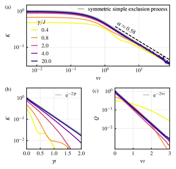
Figure 2: (a) Density autocorrelation function, Eq. (17), for occupation measurements. For $\gamma\gg J$, the dynamics agree with a symmetric simple exclusion process. The Zeno effect becomes manifest in the collapse of the data after rescaling time with $\nu=J^{2}/\gamma$. Particle number conservation causes algebraic decay $K(t)\sim t^{-\alpha}$ with $\alpha\approx 0.58$. (b) For fermion counting, the density autocorrelation function exhibits fast exponential decay, described by a random telegraph process. (c) The generalized Zeno effect is revealed by factoring out the telegraph process in Eq. (18). We observe a collapse of the telegraph-reduced autocorrelation function after rescaling time with $\nu$. For the results shown in this figure, $L=100$; in (a), the number of trajectories ranges from $N_{\mathrm{traj}}=10^{4}$ to $N_{\mathrm{traj}}=10^{3}$ for $\gamma=0.4J$ to $\gamma=20J$, and $N_{\mathrm{traj}}=10^{6}$ for the symmetric simple exclusion process; in (b) and (c), $N_{\mathrm{traj}}=5\times 10^{5}$ to $N_{\mathrm{traj}}=5\times 10^{4}$ for $\gamma=0.4J$ to $\gamma=20J$.

While frequent generalized measurements of occupation numbers induce the conventional quantum Zeno effect, electron counting at high rates leads to a generalized Zeno effect. As we explain in the following, both types of Zeno effects can be observed in the density autocorrelation function.

The simplest manifestation of the conventional quantum Zeno effect occurs in projective measurements: a single projective measurement causes the state of a quantum system to collapse to an eigenstate of the measured observable. Due to this initial collapse, repeated measurements yield the same result. If measurements are repeated at rate $\gamma$, and in between measurements there is coherent evolution with a characteristic frequency $J$, then transitions to other eigenstates of the measured observable occur at the perturbatively small rate $\nu=J^{2}/\gamma$—this suppression of coherently induced transitions is the essence of the Zeno effect.

Generalized measurements of local occupation numbers are not projective measurements. However, the measurement operators Eq. (16) are proportional to the projection operators $\hat{n}_{l}$, and, therefore, repeated measurements still induce a quantum Zeno effect. Suppose the system is prepared in a superposition of pointer states, that is, eigenstates of the measurement operators, which are classical configurations of $N$ particles on $L$ lattice sites. Then, repeated measurements gradually collapse this superposition to a single pointer state, randomly chosen according to Born’s rule. The pointer states are thus fixed points of the measurement-only dynamics. Coherent hopping destabilizes these fixed points. However, they remain metastable on a time scale $\sim 1/\nu$ [67]. Since the pointer states are classical configurations, signatures of the Zeno effect induced by generalized measurements of local occupation numbers are both emergent classicality and the suppression of coherent dynamics. This is formalized in the mapping [67] to a symmetric simple exclusion process [68, 69].

To observe these effects, we consider the average over trajectories of the conditional density autocorrelation function in the steady state, which we define with a prefactor of $4$ as

$$K(t-t^{\prime})=4\left[\overline{\left\langle\hat{n}_{l}(t)\right\rangle\left\langle\hat{n}_{l}(t^{\prime})\right\rangle}-\overline{\left\langle\hat{n}_{l}(t)\right\rangle}\;\overline{\left\langle\hat{n}_{l}(t^{\prime})\right\rangle}\right]=\overline{z_{l}(t)z_{l}(t^{\prime})}.$$ (17)

In preparation for our discussion of the generalized Zeno effect below, we have introduced an alternative representation of the density autocorrelation function in terms of the variables $z_{l}(t)=2\langle\hat{n}_{l}(t)\rangle-1$, such that an occupied or empty site corresponds to $z_{l}(t)=+1$ or $z_{l}(t)=-1$, respectively, and we consider a system with average density $\overline{\left\langle\hat{n}_{l}(t)\right\rangle}=1/2$.

Figure 2(a) shows the density autocorrelation function for generalized measurements of occupation numbers for a system of size $L=100$. For large values of $\gamma$, the data agree well with numerical simulations of the symmetric simple exclusion process with an update rate of $2\nu$ where $\nu=J^{2}/\gamma$. In particular, the initial value $K(0)$ approaches 1, which reflects that individual trajectories become dominated by pointer states, that is, classical configurations with $z_{l}(t)=\pm 1$. The suppression of coherent dynamics is demonstrated by the collapse of the data after rescaling time with $\nu=J^{2}/\gamma$. Finally, particle number conservation results in slow algebraic decay, $K(t)\sim t^{-\alpha}$. A fit to the data for $\gamma=20J$ yields $\alpha\approx 0.58$, in reasonable agreement with the diffusive scaling with $\alpha=1/2$ expected in larger systems [70]. To observe this slow decay, it is necessary to sample rare configurations with a spatially strongly inhomogeneous distribution of particles, which require long times $t\sim O(L)$ to relax and contribute significantly to the algebraic tail of $K(t)$. Therefore, to obtain the data shown in Fig. 2(a), we have initialized each trajectory in a randomly chosen classical configuration with $N=L/2$ particles.

Fermion counting can induce a generalized Zeno effect. As for the case of generalized measurements of occupation numbers, repeated application of the measurement operators Eq. (15) causes an initial superposition to collapse to a pointer state. However, the measurement operators Eq. (15) are not proportional to projection operators. Therefore, these operators do not stabilize pointer states, but rather induce transitions between pointer states. In spite of this qualitative difference, the dynamics in the frequent-measurement limit are again characterized by emergent classicality and the suppression of coherent evolution.

Figure 2(b) shows the density autocorrelation function for fermion counting. Again, $K(0)\to 1$ for increasing $\gamma$ signals that the dynamics are dominated by classical configurations. Indeed, for $\gamma=20J$, we observe good agreement with exponential decay with a rate of $2\gamma$, corresponding to a classical random telegraph process [61]. That is, the occupation of each lattice site fluctuates between zero and one at a rate $\sim\gamma$, akin to the signal produced by a telegraph. In stark contrast to the case of occupation measurements, here the measurement-only dynamics do not cause the evolution to freeze but rather to accelerate. To reveal the concomitant suppression of coherent dynamics, we consider the decay of density autocorrelations after factoring out the fast local telegraph process. This factorization can be achieved by noting that for a single realization of the telegraph process on a lattice site $l$, the density autocorrelation function can be written as $z_{l}(t)z_{l}(t^{\prime})=\left(-1\right)^{N_{l}(t,t^{\prime})}$, where $N_{l}(t,t^{\prime})$ is the fermion count at site $l$ integrated from time $t^{\prime}$ to $t$. That is, each fermion count increases $N_{l}(t,t^{\prime})$ by one and switches the sign of $z_{l}(t)$. Factoring out this classical contribution, we define the telegraph-reduced autocorrelation function as

$$Q(t-t^{\prime})=\overline{z_{l}(t)\left(-1\right)^{N_{l}(t,t^{\prime})}z_{l}(t^{\prime})}.$$ (18)

By construction, $Q(t)=1$ stays constant in the absence of coherent hopping. A nonzero hopping amplitude causes $Q(t)$ to decay, with the decay rate providing a direct measure for the suppression of coherent dynamics for large values of $\gamma$.

Figure 2(c) shows the telegraph-reduced autocorrelation function $Q(t)$. To demonstrate the suppression of coherent dynamics, we rescale time with $\nu=J^{2}/\gamma$. Indeed, for increasing $\gamma$, the data collapse to a single line. Since the number of particles is not conserved, we do not find algebraic decay, but rather exponential decay $Q(t)=\mathrm{e}^{-2\nu t}$. We interpret this slowdown of coherent dynamics for high fermion count rates as a generalized quantum Zeno effect.

To reveal the generalized Zeno effect, in Eq. (18), we had to factor out the local telegraph process for each single trajectory before taking the average over trajectories. This indicates that the generalized Zeno effect is unique to conditional dynamics under continuous monitoring, and that the suppression of coherent dynamics with an emergent slow decay rate $\nu=J^{2}/\gamma$ cannot be seen in the unconditional dynamics. To provide supporting evidence for this conjecture, we consider the density autocorrelation function defined by

$$C_{0}(t-t^{\prime})=\frac{1}{2}\overline{\left\langle\left\{\hat{n}_{l}(t),\hat{n}_{l}(t^{\prime})\right\}\right\rangle}-\overline{\left\langle\hat{n}_{l}(t)\right\rangle}\;\overline{\left\langle\hat{n}_{l}(t^{\prime})\right\rangle}.$$ (19)

Here, unconditional two-time averages are determined by the quantum regression theorem [71]. For example, for $t>t^{\prime}>t_{0}$,

$$\overline{\left\langle\hat{n}_{l}(t)\hat{n}_{l}(t^{\prime})\right\rangle}=\mathop{\mathrm{tr}}\!\left[\hat{n}_{l}\mathrm{e}^{\mathcal{L}\left(t-t^{\prime}\right)}\hat{n}_{l}\mathrm{e}^{\mathcal{L}\left(t^{\prime}-t_{0}\right)}\hat{\rho}_{0}\right],$$ (20)

where $\hat{\rho}_{0}=\lvert\psi_{0}\rangle\langle\psi_{0}\rvert$ is the projector on the initial state, and the Liouvillian $\mathcal{L}$ is defined by

$$\mathcal{L}\hat{\rho}=-\mathrm{i}\left[\hat{H},\hat{\rho}\right]+\sum_{\alpha=\pm}\sum_{l=1}^{L}\left(2\hat{L}_{\alpha,l}^{\vphantom{\dagger}}\hat{\rho}\hat{L}_{\alpha,l}^{\dagger}-\left\{\hat{L}_{\alpha,l}^{\dagger}\hat{L}_{\alpha,l}^{\vphantom{\dagger}},\hat{\rho}\right\}\right).$$ (21)

The sum over $\alpha$ is absent for occupation measurements, which are described by a single type of jump operators. Let us anticipate that within the framework of replica Keldysh field theory introduced below, we find the unconditional density autocorrelation function for occupation measurements to be given by

$$C_{0}(t)\approx\frac{1}{8\sqrt{\pi\nu\left\lvert t\right\rvert}}.$$ (22)

That is, we find slow, diffusive decay with a diffusion constant $\sim\nu$, also in the unconditional dynamics. For fermion counting, the Liouvillian, Eq. (21), is quadratic and the unconditional autocorrelation function can be calculated exactly by elementary means. The exact result is reproduced by the replica Keldysh field theory approach introduced below, which yields

$$C_{0}(t)=\frac{1}{4}\mathrm{e}^{-2\gamma\left\lvert t\right\rvert}J_{0}(2J\left\lvert t\right\rvert)^{2}\sim\frac{\mathrm{e}^{-2\gamma\left\lvert t\right\rvert}}{4\pi J\left\lvert t\right\rvert}\sin(2J\left\lvert t\right\rvert+\pi/4)^{2},$$ (23)

where $J_{0}$ is the Bessel function of the first kind and the asymptotic form applies to $\left\lvert t\right\rvert\to\infty$. As for the conditional density correlation function Eq. (17), we obtain exponential decay with a rate of $2\gamma$, and there is no indication of a suppression of coherent dynamics for $\gamma\gg J$.

Having established the suppression of coherent dynamics and emergent classicality in the conditional time evolution as common traits of the conventional and generalized Zeno effects, we now turn to the question of how these properties are reflected in correlations and entanglement in the steady state.

V Replica Keldysh field theory

In Sec. III, we have introduced two equivalent ways to describe the dynamics generated by continuous monitoring: in terms of a stochastic Schrödinger equation, and as random generalized measurements. We now focus on the latter formulation, which is a suitable starting point for making analytical progress using replica Keldysh field theory. To that end, we generalize the formalism introduced for projective measurements in Ref. [58] to generalized measurements. Our presentation closely follows Ref. [58], but we highlight new aspects that are specific to our models.

As explained in Sec. III.1, for both fermion counting and generalized occupation measurements, the unconditional steady state is completely featureless for any value of the measurement rate $\gamma$. Therefore, to observe nontrivial effects of continuous monitoring, we have to consider observables that are nonlinear in the state, such that the averaging over trajectories does not simply amount to replacing the conditional by the unconditional state. As an important example, we will study here the von Neumann entanglement entropy. For a pure state $\hat{\rho}=\lvert\psi\rangle\langle\psi\rvert$, given a bipartition of the system into a subsystem $A$ and its compliment $B$, the von Neumann entanglement entropy of subsystem $A$ reads

$$S_{A}=-\overline{\mathop{\mathrm{tr}}\!\left[\hat{\rho}_{A}\ln\!\left(\hat{\rho}_{A}\right)\right]},$$ (24)

where $\hat{\rho}_{A}=\mathop{\mathrm{tr}_{B}}(\hat{\rho})$ is the reduced density matrix of subsystem $A$. For Gaussian states, the entanglement entropy is related to the full counting statistics of the number of particles in subsystem $A$ [72, 73, 74, 75, 76],

$$S_{A}=2\sum_{k=1}^{\infty}\zeta(2k)C_{A}^{(2k)}=\frac{\pi^{2}}{3}C_{A}^{(2)}+\frac{\pi^{4}}{45}C_{A}^{(4)}+\dotsb,$$ (25)

where $\zeta(k)$ denotes the Riemann zeta function and $C_{A}^{(k)}$ is the $k$-th cumulant of the subsystem particle number $\hat{N}_{A}=\sum_{l\in A}\hat{n}_{l}$. In particular, the second cumulant is given by

$$C_{A}^{(2)}=\overline{\left\langle\left(\hat{N}_{A}-\left\langle\hat{N}_{A}\right\rangle\right)^{2}\right\rangle}.$$ (26)

The task at hand is, therefore, to calculate the average over trajectories of polynomials of quantum expectation values taken in the pure conditional state. Working toward this goal for a many-body system, we want to employ the methods provided by nonequilibrium quantum field theory to obtain an effective description in the long-wavelength limit.

V.1 Replica trick

Rewriting nonlinear observables such as the second cumulant, Eq. (26), as functional integrals in the framework of Keldysh field theory can be achieved by introducing copies or replicas of the system in two steps. First, we note that the average over trajectories of a product of $k$ expectation values can be reformulated as a single expectation value that contains the average of $k$ replicas of the density matrix. For example, for two operators $\hat{A}$ and $\hat{B}$ we can write

$$\begin{split}\overline{\left\langle\hat{A}(t)\right\rangle\left\langle\hat{B}(t)\right\rangle}&=\overline{\mathop{\mathrm{tr}}\!\left[\hat{A}\hat{\rho}(t)\right]\mathop{\mathrm{tr}}\!\left[\hat{B}\hat{\rho}(t)\right]}\\ &=\mathop{\mathrm{tr}}\!\left\{\left(\hat{A}_{1}\otimes\hat{B}_{2}\right)\overline{\left[\hat{\rho}_{1}(t)\otimes\hat{\rho}_{2}(t)\right]}\right\}.\end{split}$$ (27)

In the last equality, we have introduced the replica index $r\in\{1,2\}$ to indicate on which copy of the system a particular operator is acting. Generalizing the above relation, a product of $k$ expectation values can be expressed in terms of the $k$-replica density matrix

$$\hat{\mu}_{k}(t)=\overline{\bigotimes_{r=1}^{k}\hat{\rho}_{r}(t)}.$$ (28)

In the formulation of our models in terms of random generalized measurements, the overbar denotes the average over measurement times $t_{m}$ and measurement outcomes $l_{m}\in\{1,\dotsc,L\}$ and $\alpha_{m}\in\{+,-\}$, where the former is the measured lattice site and the distinction between possible jumps in the latter is only required for fermion counting but not for occupation measurements. We emphasize that treating generalized occupation measurements requires us to consider the site indices $l_{m}$ as measurement outcomes, which is not the case for the projective measurements studied in Ref. [58].

A particular sequence of measurement outcomes is realized with a probability that can be expressed in terms of the nonnormalized density matrix for a single copy of the system. If we omit the normalization factor in Eq. (1), the state of the system after a time $t$ can be written as

$$\hat{D}(t)=\hat{V}(t)\hat{\rho}_{0}\hat{V}(t)^{\dagger},$$ (29)

with the initial state $\hat{\rho}_{0}=\lvert\psi_{0}\rangle\langle\psi_{0}\rvert$ and where

$$\hat{V}(t)=\hat{U}(t-t_{M})\hat{M}_{\alpha_{M},l_{M}}\hat{U}(t_{M}-t_{M-1})\dotsb\hat{M}_{\alpha_{1},l_{1}}\hat{U}(t_{1}-t_{0}).$$ (30)

In $\hat{V}(t)$, unitary evolution $\hat{U}(t)=\mathrm{e}^{-\mathrm{i}\hat{H}t}$ is interspersed with quantum jumps $\hat{M}_{\alpha_{m},l_{m}}$ at times $t_{m}$ with $m\in\{1,\dots,M\}$. We leave the dependence of $\hat{V}(t)$ on the sequence of measurement outcomes and times $\{\alpha_{m},l_{m},t_{m}\}$ implicit. The normalized density matrix is obtained by reinstating the factors $p_{\alpha_{m},l_{m}}(t)$ in Eq. (1), leading to

$$\hat{\rho}(t)=\frac{1}{\prod_{m=1}^{M}p_{\alpha_{m},l_{m}}(t_{m})}\hat{D}(t).$$ (31)

Finally, using that $\mathop{\mathrm{tr}}(\hat{\rho}(t))=1$, we obtain the probability to obtain the entire sequence of measurement outcomes, given by the product of probabilities of individual measurement outcomes, as

$$p_{\{\alpha_{m},l_{m}\}}(\{t_{m}\})=\prod_{m=1}^{M}p_{\alpha_{m},l_{m}}(t_{m})=\mathop{\mathrm{tr}}\!\left[\hat{D}(t)\right].$$ (32)

With this expression for the probability of a given sequence $\{\alpha_{m},l_{m}\}$ of measurement outcomes, we can write the average over trajectories in Eq. (28) as

$$\hat{\mu}_{k}(t)=\sum_{\{\alpha_{m},l_{m},t_{m}\}}\left.\left[\bigotimes_{r=1}^{k}\hat{D}_{r}(t)\right]\middle/\mathop{\mathrm{tr}}\!\left[\hat{D}(t)\right]^{k-1}\right.,$$ (33)

where the symbolic sum includes the average over both the Poisson distribution of the number of measurements $M$ in the time interval of length $T=t-t_{0}$ and the uniform distribution of measurement times:

$$\sum_{\{\alpha_{m},l_{m},t_{m}\}}=\sum_{M=0}^{\infty}\frac{\left(\gamma LT\right)^{M}\mathrm{e}^{-\gamma LT}}{M!}\prod_{m=1}^{M}\sum_{\alpha_{m}=\pm}\sum_{l_{m}=1}^{L}\int_{t_{0}}^{t}\frac{\mathrm{d}t_{m}}{T}.$$ (34)

The denominator in Eq. (33) obstructs the application of the usual Keldysh construction to obtain a functional integral representation of the time evolution of the $k$-replica density matrix. We can get rid of this denominator by using the replica trick, which amounts here to first introducing additional replicas with indices $r\in\{k+1,\dotsc,R\}$ and then taking the replica limit $R\to 1$:

$$\hat{\mu}_{k}(t)=\lim_{R\to 1}\sum_{\{\alpha_{m},l_{m},t_{m}\}}\mathop{\mathrm{tr}_{r=k+1,\dotsc,R}}\!\left[\bigotimes_{r=1}^{R}\hat{D}_{r}(t)\right].$$ (35)

As pointed out in Refs. [16, 36, 58], the probability in Eq. (32) according to Born’s rule is reproduced in the replica limit $R\to 1$, different from the usual replica limit $R\to 0$ in the theory of disordered systems.

Through the above formal manipulations, we can now obtain averages over trajectories of nonlinear observables such as the cumulant, Eq. (26), by calculating expectation values that are linear in the nonnormalized density matrix of $R$ replicas of the original system and taking the replica limit $R\to 1$ in the end. Note that the way in which we have introduced replicas in Eq. (27) allows us to obtain equal-time correlations of conditional expectation values $\left\langle\hat{A}(t)\right\rangle$ and $\left\langle\hat{B}(t)\right\rangle$. However, unconditional averages, such as the autocorrelation function, Eq. (19), can also be obtained for operators $\hat{A}(t)$ and $\hat{B}(t^{\prime})$ at different times $t\neq t^{\prime}$. As usual, a convenient way to generate different forms of expectation values is by introducing source terms in the $R$-replica Keldysh partition function,

$$Z_{R}(t)=\sum_{\{\alpha_{m},l_{m},t_{m}\}}\mathop{\mathrm{tr}}\!\left[\bigotimes_{r=1}^{R}\hat{D}_{r}(t)\right].$$ (36)

By construction, the $R$-replica Keldysh partition function is normalized such that $Z_{R}(t)\to 1$ for $R\to 1$. We proceed to derive a functional integral representation of $Z_{R}(t)$, where source fields can be introduced as required at a later stage.

V.2 Replica Keldysh action

In Keldysh field theory [77, 78, 79, 80], the $R$-replica Keldysh partition function, Eq. (36), is expressed as a functional integral over two independent sets of Grassmann fields $\psi_{k,r,l}(t)$ and $\bar{\psi}_{k,r,l}(t)$ with Keldysh index $k$ and replica index $r$, which we collect into $2R$-component vectors denoted by $\psi_{l}(t)$ and $\bar{\psi}_{l}(t)$. Time evolution of the nonnormalized density matrix, Eq. (29), is visualized as proceeding along two branches, the forward branch described by $\hat{V}(t)$ acting on $\hat{\rho}_{0}$ from the left, and the backward branch described by $\hat{V}(t)^{\dagger}$ acting on $\hat{\rho}_{0}$ from the right. Replacing operators on the forward and backward branches by fields with Keldysh indices $k=+$ and $k=-$, respectively, we obtain

$$Z_{R}(t)=\int\mathrm{D}[\bar{\psi},\psi]\,\mathrm{e}^{\mathrm{i}\bar{\psi}G_{0}^{-1}\psi}\\ \times\sum_{\{\alpha_{m},l_{m},t_{m}\}}\prod_{r=1}^{R}M_{+,r,\alpha_{m},l_{m}}(t_{m})M_{-,r,\alpha_{m},l_{m}}^{\dagger}(t_{m}).$$ (37)

We omit the matrix element of the initial state $\hat{\rho}_{0}$, which fixes the number of particles for occupation measurements but is otherwise irrelevant in the steady state, which can be described by taking the limit $t_{0}\to-\infty$. Unitary evolution contained in $\hat{V}(t)$, Eq. (30), gives rise to the quadratic Keldysh action, where we use a shorthand notation leaving the integration over time and summation over lattice sites implicit,

$$\bar{\psi}G_{0}^{-1}\psi=\int_{t_{0}}^{t}\mathrm{d}t^{\prime}\sum_{l,l^{\prime}=1}^{L}\bar{\psi}_{l}(t^{\prime})G_{0,l,l^{\prime}}^{-1}\psi_{l^{\prime}}(t^{\prime}).$$ (38)

The inverse Green’s function reads $G_{0}^{-1}=\left(\mathrm{i}\partial_{t}-H\right)\sigma_{z}$, where $\sigma_{z}$ is a Pauli matrix in Keldysh space and the matrix $H_{l,l^{\prime}}=-J\left(\delta_{l+1,l^{\prime}}+\delta_{l,l^{\prime}+1}\right)$ describes hopping according to Eq. (2). To further simplify the notation, we omit the identity $1_{R}$ in replica space in the definition of the Green’s function. In the limit $t_{0}\to-\infty$, the Green’s function should be augmented by an infinitesimal regularization term, fixing the correct causality properties and particle number [58]. We omit this term since the Green’s function will be dressed due to measurements.

According to the rule formulated above for replacing operators by fields, the measurement operators for fermion counting, Eq. (15), are represented by

$$\begin{split}M_{\pm,r,-,l}(t)&=M_{\pm,r,+,l}^{\dagger}(t)=\pm\frac{1}{\sqrt{L}}\psi_{\pm,r,l}(t),\\ M_{\pm,r,+,l}(t)&=M_{\pm,r,-,l}^{\dagger}(t)=\pm\frac{1}{\sqrt{L}}\bar{\psi}_{\pm,r,l}(t),\end{split}$$ (39)

where we include the minus sign acquired by Grassmann fields on the backward branch [80]. For the measurement operators describing generalized measurements of occupation numbers, Eq. (16), we obtain

$$M_{\pm,r,l}(t)=M_{\pm,r,l}^{\dagger}(t)=\frac{1}{\sqrt{N}}\bar{\psi}_{\pm,r,l}(t)\psi_{\pm,r,l}(t).$$ (40)

We can now perform the average over the Poisson distribution of the number of measurements included in Eq. (34). Then, the product over fields representing the measurement operators in Eq. (37) gets exponentiated, such that $Z_{R}(t)=\int\mathrm{D}[\bar{\psi},\psi]\mathrm{e}^{\mathrm{i}S[\bar{\psi},\psi]}$, where the action reads

$$S[\bar{\psi},\psi]=\int_{t_{0}}^{t}\mathrm{d}t^{\prime}\sum_{l,l^{\prime}=1}^{L}\bar{\psi}_{l}G_{0,l,l^{\prime}}^{-1}\psi_{l^{\prime}}+\gamma\int\mathrm{d}^{2}\mathbf{x}\,\mathcal{L}_{M}[\bar{\psi}_{l},\psi_{l}].$$ (41)

Here and occasionally in the following, we abbreviate expressions by omitting lattice indices and time arguments; further, we abbreviate integration over space and time as $\int\mathrm{d}^{2}\mathbf{x}=\sum_{l=1}^{L}\int_{t_{0}}^{t}\mathrm{d}t^{\prime}$. The Lagrangian density due to random generalized measurements reads

$$\mathrm{i}\mathcal{L}_{M}[\bar{\psi},\psi]=\sum_{\alpha=\pm}\prod_{r=1}^{R}V_{\alpha}[\bar{\psi}_{r},\psi_{r}]-1,$$ (42)

where vertices $V_{\alpha}[\bar{\psi},\psi]$ for fermion counting are given by

$$V_{-}[\bar{\psi}_{r},\psi_{r}]=-\psi_{+,r}\bar{\psi}_{-,r},\qquad V_{+}[\bar{\psi}_{r},\psi_{r}]=-\bar{\psi}_{+,r}\psi_{-,r}.$$ (43)

For occupation measurements, there is a single vertex that depends explicitly on the fermion density $n=N/L$,

$$V[\bar{\psi}_{r},\psi_{r}]=\frac{1}{n}\bar{\psi}_{+,r}\psi_{+,r}\bar{\psi}_{-,r}\psi_{-,r}.$$ (44)

As outlined above, the translation from the operator formalism to a functional-integral formulation is achieved most transparently in the basis of fields on the forward and backward branch. However, for what follows it is more convenient to perform a Larkin-Ovchinnikov rotation [77, 78],

$$\psi_{1,2}=\frac{1}{\sqrt{2}}\left(\psi_{+}\pm\psi_{-}\right),\qquad\bar{\psi}_{1,2}=\frac{1}{\sqrt{2}}\left(\bar{\psi}_{+}\mp\bar{\psi}_{-}\right).$$ (45)

In this basis, the bare Green’s function is proportional to the identity in both Keldysh and replica spaces, $G_{0}^{-1}=\mathrm{i}\partial_{t}-H$.

The replica Keldysh construction we have presented above provides an exact reformulation of the dynamics under continuous monitoring as a field theory. To make further progress, we now have to introduce suitable approximations. The first step is to identify the relevant degrees of freedom, which dominate correlations and—via Eq. (25)—the dynamics of entanglement at long wavelengths. For generalized measurements of occupation numbers, we expect that the relevant slow modes are the same as for the case of projective measurements, that is, fermionic bilinears which we collect in the matrix $\mathcal{G}_{l}(t)=-\mathrm{i}\psi_{l}(t)\bar{\psi}_{l}(t)$ [58]. As we will see comparing with our numerical results, this turns out to be the correct choice also for fermion counting.

Specifically, we want $\left\langle\mathcal{G}_{l}(t)\right\rangle$ to represent the fermionic Green’s function at equal positions and in the symmetrized limit of equal time arguments of the fields $\psi_{l}(t)$ and $\bar{\psi}_{l}(t)$,

$$\left\langle\mathcal{G}_{l}(t)\right\rangle=-\frac{\mathrm{i}}{2}\left(\left\langle\psi_{l}(t)\bar{\psi}_{l}(t+0^{+})\right\rangle+\left\langle\psi_{l}(t)\bar{\psi}_{l}(t-0^{+})\right\rangle\right).$$ (46)

Two technical issues arise: (i) in the construction of the Keldysh field integral, which is based on a discretization of time, products of field operators $\hat{n}_{l}=\hat{\psi}_{l}^{\dagger}\hat{\psi}_{l}$ as occur in the measurement operators for occupation measurements in Eq. (16) are replaced by fields that are a discrete time step apart; (ii) the discrete-time Green’s function at equal discrete times differs from the symmetrized limit of equal time arguments in the continuous-time formulation [78], and we want $\left\langle\mathcal{G}_{l}(t)\right\rangle$ to represent the latter. These discrepancies can be resolved by using the regularization procedure detailed in Appendix B.

The measurement operators for fermion counting are linear in fermionic field operators. Therefore, in this case, the issues described above do not arise, and the vertices in Eq. (43) are not affected by the regularization. After the Larkin-Ovchinnikov rotation, these vertices take the form

$$V_{\pm}[\bar{\psi},\psi]=-\frac{1}{2}\left[\bar{\psi}_{1}\psi_{1}-\bar{\psi}_{2}\psi_{2}\mp\left(\bar{\psi}_{1}\psi_{2}-\bar{\psi}_{2}\psi_{1}\right)\right].$$ (47)

In contrast, through the regularization we obtain a modified vertex for generalized measurements of occupation numbers,

$$V[\bar{\psi},\psi]=\frac{1}{n}\left[\frac{1}{4}+\frac{1}{2}\left(\bar{\psi}_{1}\psi_{2}+\bar{\psi}_{2}\psi_{1}\right)-\bar{\psi}_{1}\psi_{1}\bar{\psi}_{2}\psi_{2}\right],$$ (48)

Up to the prefactor $1/n$, the regularized vertex is identical to one of the regularized vertices for projective occupation measurements of Ref. [58].

The vertices in Eqs. (47) and (48) contain the term $\bar{\psi}_{2}\psi_{1}$, which would correspond to an anti-Keldysh component of the self-energy, and thus violates the familiar causality structure of fermionic Keldysh field theory [78]. For fermion counting and in the replica limit $R\to 1$, this term cancels in the sum over $\alpha$ in Eq. (42). However, this is not the case for occupation measurements. In Appendix B, we discuss how the appearance of an anti-Keldysh component can be reconciled with the normalization of the Keldysh partition function in the replica limit, $Z_{R}(t)\to 1$ for $R\to 1$. The violation of the usual causality structure is only due to the part of the Lagrangian for occupation measurements that is quadratic in fermionic fields,

$$\mathrm{i}\mathcal{L}_{M,Q}[\bar{\psi},\psi]=\frac{1}{2^{2R-1}n^{R}}\sum_{r=1}^{R}\left(\bar{\psi}_{1,r}\psi_{2,r}+\bar{\psi}_{2,r}\psi_{1,r}\right),$$ (49)

which we therefore separate from the nonquadratic part, $\mathcal{L}_{M,\mathit{NQ}}=\mathcal{L}_{M}-\mathcal{L}_{M,Q}$. To preserve the usual structure of the Keldysh formalism, we will treat $\mathcal{L}_{M,Q}$ perturbatively, so that the self-energy, which nonperturbatively dresses the Green’s function, is fully determined by $\mathcal{L}_{M,\mathit{NQ}}$. For brevity, we will drop the subscript $\mathit{NQ}$ in the following.

With these precautions, we introduce Hermitian $2R\times 2R$ matrix fields $\mathcal{G}$ and $\Sigma$, corresponding to the equal-time fermionic Green’s function and the self-energy, by means of a generalized Hubbard-Stratonovich transformation [58]. That is, we include the factor

$$1=\int\mathrm{D}[\mathcal{G},\Sigma]\,\mathrm{e}^{-\frac{\epsilon}{2}\mathop{\mathrm{Tr}}\left(\Sigma^{2}\right)-\mathrm{i}\mathop{\mathrm{Tr}}\left(\mathcal{G}\Sigma\right)-\bar{\psi}\Sigma\psi}$$ (50)

in the functional integral over $\psi$ and $\bar{\psi}$. The trace $\mathop{\mathrm{Tr}}\!\left(\,\cdot\,\right)$ acts in Keldysh, replica, lattice, and time spaces, with the matrices $\mathcal{G}$ and $\Sigma$ being diagonal in lattice and time spaces. Convergence of the integration over $\mathcal{G}$ and $\Sigma$ is ensured by the term proportional to $\epsilon$. We omit this term in the following, with the understanding that the limit $\epsilon\to 0$ has to be taken at the end of the calculation. In this limit, the integral over $\Sigma$ reduces to a delta functional fixing $\mathcal{G}=-\mathrm{i}\psi\bar{\psi}$ [58]. Using this relation, decoupling the measurement Lagrangian simultaneously in all possible slow channels is achieved by taking the average of $\mathcal{L}_{M}$ with respect to the Gaussian action $\bar{\psi}\mathcal{G}^{-1}\psi$ [58]. For fermion counting, this is done most conveniently with the form of the vertices given in Eq. (43), and the result can be expressed as a trace $\mathop{\mathrm{tr}_{K}}$ in Keldysh space and a determinant $\mathop{\mathrm{det}_{R}}$ in replica space,

$$\mathrm{i}\mathcal{L}_{M}[\mathcal{G}]=\sum_{\alpha=\pm}\mathop{\mathrm{det}_{R}}\!\left[\mathop{\mathrm{tr}_{K}}\!\left(\tau_{\alpha}\mathcal{G}\right)\right]-1,$$ (51)

where $\tau_{\pm}=(\mathrm{i}\sigma_{z}\pm\sigma_{y})/2$ and $\sigma_{i}$ are the Pauli matrices. The Lagrangian for occupation measurements contains a determinant $\det(\,\cdot\,)$ and a trace $\mathop{\mathrm{tr}}(\,\cdot\,)$ in both Keldysh and replica spaces,

$$\mathrm{i}\mathcal{L}_{M}[\mathcal{G}]=\frac{1}{n^{R}}\mathop{\mathrm{det}}\!\left(\frac{1}{2}-\mathrm{i}\sigma_{x}\mathcal{G}\right)+\frac{\mathrm{i}}{2^{2R-1}n^{R}}\mathop{\mathrm{tr}}\!\left(\sigma_{x}\mathcal{G}\right)-1.$$ (52)

This form of the measurement Lagrangian is similar to the one for projective measurements [58]: the latter does not contain the prefactor $1/n^{R}$ and the two types of projection operators, $\hat{n}_{l}$ and $1-\hat{n}_{l}$, result in two determinant contributions with opposite signs of the term containing $\mathcal{G}$, in contrast to our model with only one determinant term. The trace in Eq. (52) stems from the subtraction of $\mathcal{L}_{M,Q}$, Eq. (49), and ensures that $\mathcal{L}_{M}$ does not contain terms that are linear in $\mathcal{G}$.

After decoupling the measurement Lagrangian, the action is quadratic in the fermionic fields $\psi$ and $\bar{\psi}$, which can thus be integrated out, leading to

$$S[\mathcal{G},\Sigma]=S_{0}[\mathcal{G},\Sigma]+\gamma\int\mathrm{d}^{2}\mathbf{x}\,\mathcal{L}_{M}[\mathcal{G}_{l}],$$ (53)

where

$$\mathrm{i}S_{0}[\mathcal{G},\Sigma]=\mathop{\mathrm{Tr}}\!\left\{\ln\!\left[G_{0}^{-1}+\mathrm{i}\left(\Sigma+A\right)\right]-\mathrm{i}\mathcal{G}\Sigma\right\}.$$ (54)

The matrix $A$ results from expressing the quadratic part of the measurement action, Eq. (49), as

$$\mathrm{i}\gamma\int\mathrm{d}^{2}\mathbf{x}\,\mathcal{L}_{M,Q}[\bar{\psi}_{l},\psi_{l}]=-\bar{\psi}A\psi,$$ (55)

where $A=0$ for fermion counting and, for occupation measurements,

$$A=-\frac{\gamma}{2^{2R-1}n^{R}}\sigma_{x}.$$ (56)

As anticipated, we treat $A\sim\gamma$ perturbatively. To first order in $A$, the action in Eq. (54) reads

$$\mathrm{i}S_{0}[\mathcal{G},\Sigma]=\mathop{\mathrm{Tr}}\!\left[\ln\!\left(G^{-1}\right)+\mathrm{i}\left(GA-\mathcal{G}\Sigma\right)\right],$$ (57)

where the dressed Green’s function is given by

$$G^{-1}=G_{0}^{-1}+\mathrm{i}\Sigma.$$ (58)

V.3 Symmetries of the Keldysh action

The long-wavelength behavior of our models is dominated by strong fluctuations of soft modes, which are related to symmetries of the Keldysh action. Therefore, a prerequisite for deriving a long-wavelength effective field theory is to identify the relevant symmetries. This analysis provides important insights into the consequences of particle number conservation for generalized occupation measurements.

The fermionic replica Keldysh action in Eq. (41) is defined in terms of $2R$-component vectors of Grassmann fields $\psi$ and $\bar{\psi}$. In the Larkin-Ovchinnikov basis, Eq. (45), the bare Green’s function $G_{0}$ is diagonal in Keldysh and replica spaces, and, therefore, rotations of the fields described by $\psi\mapsto\mathcal{R}\psi$ and $\bar{\psi}\mapsto\bar{\psi}\mathcal{R}^{-1}$ with $\mathcal{R}\in\mathrm{U}(2R)$ leave the first term in the action of Eq. (41), which encodes free evolution in the absence of measurements, invariant. Which rotations are symmetries of the full action including the measurement Lagrangian is most conveniently analyzed after performing the generalized Hubbard-Stratonovich transformation, that is, for the action in Eq. (57) and the measurement Lagrangians given in Eqs. (51) and (52) in terms of the matrix fields $\mathcal{G}$ and $\Sigma$. Rotations of the fermionic fields act on the matrix fields as $\mathcal{G}\mapsto\mathcal{R}\mathcal{G}\mathcal{R}^{-1}$ and $\Sigma\mapsto\mathcal{R}\Sigma\mathcal{R}^{-1}$. Interestingly, the measurement Lagrangians have different symmetries for $R=1$ and $R>1$, corresponding to the unconditional evolution of observables that are linear in the system state and to the conditional evolution of nonlinear observables, respectively.

We consider first the case $R=1$. Then, the measurement Lagrangian for fermion counting, Eq. (51), reduces to

$$\mathrm{i}\mathcal{L}_{M}[\mathcal{G}]=\mathrm{i}\mathop{\mathrm{tr}_{K}}\!\left(\sigma_{z}\mathcal{G}\right)-1.$$ (59)

This Lagrangian and the action in Eq. (57), where $A=0$ for fermion counting, are invariant under phase rotations $\mathcal{R}_{\eta}=\mathrm{e}^{\mathrm{i}\eta/2}$ and $\mathcal{R}_{\zeta}=\mathrm{e}^{\mathrm{i}\zeta\sigma_{z}/2}$, with $\eta,\zeta\in\mathbb{R}$. For occupation measurements, the Lagrangian Eq. (52) simplifies for $R=1$ to

$$\mathrm{i}\mathcal{L}_{M}[\mathcal{G}]=\frac{1}{n}\left[\frac{1}{4}+\mathop{\mathrm{det}_{K}}(\mathcal{G})\right]-1,$$ (60)

which is invariant under arbitrary rotations $\mathcal{R}\in\mathrm{U}(2)$. However, the matrix $A$, Eq. (56), appearing in the action in Eq. (57) is proportional to $\sigma_{x}$, thus reducing the symmetries of the action to rotations of the form $\mathcal{R}_{\eta}$ and $\mathcal{R}_{\phi}=\mathrm{e}^{\mathrm{i}\phi\sigma_{x}/2}$. An inverse Larkin-Ovchinnikov rotation, Eq. (45), shows that the transformation $\mathcal{R}_{\phi}$ corresponds to phase rotations with opposite signs on the forward and backward branches of the Keldysh contour, which is the quantum [79, 80] or strong symmetry [81] that is associated with particle number conservation.

We now turn to the case $R>1$. Surprisingly, there is now an additional type of rotations which is a symmetry of the action, Eq. (57), and the measurement Lagrangian, Eq. (51), for fermion counting, given by $\mathcal{R}_{\Phi}=\mathrm{e}^{\mathrm{i}\Phi\sigma_{x}/2}$ where $\Phi$ is a traceless $R\times R$ matrix. We show that $\mathcal{R}_{\Phi}$ is a symmetry of Eq. (57) in Appendix C. For the case of occupation measurements, it is obvious from inspection of Eqs. (52) and (57) with (56) that rotations of the form $\mathcal{R}_{\Phi}$ are a symmetry.

V.4 Saddle-point manifold

The field integral over $\mathcal{G}$ and $\Sigma$ is dominated by the spatially homogeneous and time-independent saddle points of the Keldysh action. Due to the symmetries of the Keldysh action discussed in the previous section, there is, in fact, a manifold of saddle points. To establish the manifold, it is sufficient to find one particular saddle point. The full manifold is then obtained by applying all rotations that are symmetries of the action to the particular saddle point.

We consider first the variation of the action with respect to $\Sigma$, which yields the saddle-point equation

$$\mathcal{G}=\int_{-\infty}^{\infty}\frac{\mathrm{d}\omega}{2\pi}\int_{-\pi}^{\pi}\frac{\mathrm{d}q}{2\pi}\frac{1}{\omega-\xi_{q}+\mathrm{i}\Sigma},$$ (61)

where $\xi_{q}=-2J\cos(q)$ is the dispersion relation of the Hamiltonian in Eq. (2). We omit a contribution to the saddle point of $\mathcal{G}$ that contains $A$. Since $\Sigma\sim\gamma$ at the saddle point as shown below, such a contribution would lead to terms of second order in $\gamma$ when we insert $\mathcal{G}$ in the action Eq. (57). In accordance with Eq. (46), the integration over frequencies in Eq. (61) has to be regularized by introducing a factor $\bigl{(}\mathrm{e}^{\mathrm{i}\omega t}+\mathrm{e}^{-\mathrm{i}\omega t}\bigr{)}\big{/}2$, where the limit $t\to 0^{+}$ is taken after the integration. By writing $\Sigma=\mathcal{V}\lambda\mathcal{V}^{-1}$, where $\lambda$ is a diagonal matrix, we thus find [58]

$$\mathcal{G}=-\mathrm{i}Q/2,\quad Q=\mathop{\mathrm{sgn}}\!\left[\mathop{\mathrm{Re}}(\Sigma)\right]=\mathcal{V}\mathop{\mathrm{sgn}}\!\left[\mathop{\mathrm{Re}}(\lambda)\right]\mathcal{V}^{-1}.$$ (62)

Note that the matrix $Q$ obeys the nonlinear constraint $Q^{2}=1$.

To simplify the analysis of the saddle-point equation that follows from the variation of the action with respect to $\mathcal{G}$, we use that—as explained above—to establish the full manifold of saddle points, it is sufficient to find one particular saddle point. We thus focus on replica-symmetric saddle points, $Q=Q_{0}\otimes 1_{R}$. Equation (46) suggests that a particular solution of the saddle-point equation for $\mathcal{G}$ is given by the symmetrized equal-time limit of the Green’s function, which, as discussed in Appendix B, is fully determined by fermionic anticommutation relations and the distribution function $\left\langle\hat{n}_{l}\right\rangle_{\mathrm{ss}}=n$ in the steady state. This particular solution is obtained from Eq. (62) by setting $\Sigma\propto\Lambda$, leading to $Q_{0}=\Lambda$ where

$$\Lambda=\begin{pmatrix}1&2\left(1-2n\right)\\ 0&-1\end{pmatrix}$$ (63)

with $n=1/2$, such that $\Lambda=\sigma_{z}$ for fermion counting. The variation of the action with respect to $\mathcal{G}$ can be obtained conveniently by inserting $\mathcal{G}=-\mathrm{i}\left(Q_{0}+\delta Q_{\mathcal{G}}\right)\!\big{/}2$ in the measurement Lagrangian and performing an expansion in $\delta Q_{\mathcal{G}}$ as detailed in Appendix D. Accounting for the symmetries of the Keldysh action discussed in Sec. V.3, we then obtain the manifold of saddle points for fermion counting:

$$\Sigma=\gamma Q/2^{R-1},\qquad Q=\mathcal{R}_{\Phi}\sigma_{z}\mathcal{R}_{\Phi}^{-1}.$$ (64)

The symmetries of the Keldysh action $\mathcal{R}_{\eta}$ and $\mathcal{R}_{\zeta}$ do not rotate the saddle point, and, therefore, do not further enlarge the saddle-point manifold. Note that the relation between $\Sigma$ and $Q$ is consistent with the definition of $Q$ in Eq. (62). For occupation measurements, we find

$$\Sigma=\gamma Q/(2n),\qquad Q=\mathcal{R}_{\Phi}\mathcal{R}_{\phi}\Lambda\mathcal{R}_{\phi}^{-1}\mathcal{R}_{\Phi}^{-1}.$$ (65)

Here, we omit a shift of the saddle point that vanishes in the replica limit $R\to 1$ and is given explicitly in Appendix D.

Each particular saddle point in the manifold spontaneously breaks the symmetries of the Keldysh action under $\mathcal{R}_{\Phi}$ and, for occupation measurements, also $\mathcal{R}_{\phi}$. This gives rise to Goldstone modes. The Goldstone mode associated with $\mathcal{R}_{\phi}$ leads to the slow algebraic decay of the unconditional density autocorrelation function Eq. (22) for occupation measurements. In contrast, for fermion counting, there are no Goldstone modes in the replica limit $R\to 1$ that describes the unconditional dynamics—by definition, the traceless $R\times R$ matrix $\Phi$ reduces to $\Phi=0$ in this case. The absence of Goldstone modes is reflected in the exponential decay of the autocorrelation function in Eq. (23). However, as we discuss further below, the Goldstone mode associated with $\mathcal{R}_{\Phi}$ is described by the same long-wavelength effective theory for both fermion counting and occupation measurements, leading to almost identical correlations and entanglement properties in the steady state.

VI Gaussian theory

Properly treating strong massless fluctuations within the saddle-point manifold requires an RG analysis of the corresponding NLSM. However, first important insights can be obtained from considering quadratic fluctuations of $\mathcal{G}$ and $\Sigma$ around a particular saddle point within the manifold. A convenient expansion point is given by $Q=\Lambda$, where $n=1/2$ such that $\Lambda=\sigma_{z}$ for fermion counting. The Gaussian approximation is controlled for $\gamma\ll J$ and valid up to intermediate length scales, where renormalization corrections are small.

VI.1 Expansion in fluctuations

Arbitrary fluctuations around the saddle point $Q=\Lambda$ can be parametrized as

$$\mathcal{G}=-\mathrm{i}\left(\Lambda+\delta Q_{\mathcal{G}}{}\right)\!\big{/}2,\qquad\Sigma=\gamma\left(\Lambda+\delta Q_{\Sigma}{}\right)\!\big{/}(2n),$$ (66)

with Hermitian $2R\times 2R$ matrices $\delta Q_{\mathcal{G}}$ and $\delta Q_{\Sigma}$. For simplicity, we set $R=1$ in all numerical factors. Then, the expansion point for $\Sigma$ lies within the manifold for both fermion counting, Eq. (64), and occupation measurements, Eq. (65), when we set $n=1/2$ for fermion counting. As detailed in Appendix D, the Keldysh action vanishes to zeroth order in fluctuations, and there are no contributions to first order for an expansion around a saddle point. At second order, we find

$$S^{(2)}=S_{0}^{(2)}+\gamma\int\mathrm{d}^{2}\mathbf{x}\,\mathcal{L}_{M}^{(2)},$$ (67)

where [58]

$$\mathrm{i}S_{0}^{(2)}=\frac{1}{\left(4\tau_{0}\right)^{2}}\int\mathrm{d}^{2}\mathbf{x}\,\mathrm{d}^{2}\mathbf{x}^{\prime}\,\mathcal{B}_{l-l^{\prime}}(t-t^{\prime})\\ \times\mathop{\mathrm{Tr}}\!\left[\delta Q_{\Sigma,l}(t)\left(1+\Lambda\right)\delta Q_{\Sigma,l^{\prime}}(t^{\prime})\left(1-\Lambda\right)\right]\\ -\frac{1}{4\tau_{0}}\int\mathrm{d}^{2}\mathbf{x}\mathop{\mathrm{Tr}}\!\left[\delta Q_{\Sigma,l}(t)\delta Q_{\mathcal{G},l}(t)\right],$$ (68)

with the mean free time $\tau_{0}=n/\gamma$ and the block of the diffusion ladder, which, in momentum and frequency space, reads

$$\mathcal{B}_{q}(\omega)=\left\{\left(\mathrm{i}\omega-1/\tau_{0}\right)^{2}+\left[4J\sin(q/2)\right]^{2}\right\}^{-1/2}.$$ (69)

The expansion of the measurement Lagrangian is carried out in Appendix D. There are two contributions,

$$\mathcal{L}_{M}^{(2)}=\mathcal{L}_{M}^{(2,1)}+\mathcal{L}_{M}^{(2,2)}.$$ (70)

For fermion counting, the first contribution contains the trace of a square and the second contribution the square of a trace,

$$\begin{split}\mathrm{i}\gamma\mathcal{L}_{M}^{(2,1)}&=-\frac{1}{16\tau_{0}}\mathop{\mathrm{Tr}}\!\left[\Bigl{(}\sigma_{z}\delta Q_{\mathcal{G}}\Bigr{)}^{2}-\left(\sigma_{y}\delta Q_{\mathcal{G}}\right)^{2}\right],\\ \mathrm{i}\gamma\mathcal{L}_{M}^{(2,2)}&=\frac{1}{16\tau_{0}}\left[\mathop{\mathrm{Tr}}\Bigl{(}\sigma_{z}\delta Q_{\mathcal{G}}\Bigr{)}^{2}-\mathop{\mathrm{Tr}}\!\left(\sigma_{y}\delta Q_{\mathcal{G}}\right)^{2}\right].\end{split}$$ (71)

Similarly, for generalized occupation measurements we find

$$\begin{split}\mathrm{i}\gamma\mathcal{L}_{M}^{(2,1)}&=-\frac{1}{32n\tau_{0}}\mathop{\mathrm{Tr}}\!\left\{\left[\left(\Lambda-\sigma_{x}\right)\delta Q_{\mathcal{G}}\right]^{2}\right\},\\ \mathrm{i}\gamma\mathcal{L}_{M}^{(2,2)}&=\frac{1}{32n\tau_{0}}\mathop{\mathrm{Tr}}\!\left[\left(\Lambda-\sigma_{x}\right)\delta Q_{\mathcal{G}}\right]^{2}.\end{split}$$ (72)

At this point, it is useful to decompose the fluctuation matrices into longitudinal or replica-symmetric and transversal or replicon modes according to

$$\delta Q=\delta Q^{\parallel}\otimes 1_{R}+\delta Q^{\perp},$$ (73)

where, by construction, $\delta Q^{\parallel}=\left(1/R\right)\mathop{\mathrm{tr}_{R}}(\delta Q)$ and $\delta Q^{\perp}=\delta Q-\delta Q^{\parallel}\otimes 1_{R}$. These modes are orthogonal,

$$\mathop{\mathrm{tr}_{R}}\!\left[\left(\delta Q^{\parallel}\otimes 1_{R}\right)\delta Q^{\perp}\right]=0,$$ (74)

and, therefore, the theory splits into two sectors, $Z_{R}=Z_{R}^{\parallel}Z_{R}^{\perp}$. The replica-symmetric and replicon sectors describe, respectively, unconditional and conditional correlation functions.

VI.2 Density correlations

We consider two types of connected density correlation functions: the unconditional dynamics are described by

$$C_{0,l,l^{\prime}}(t,t^{\prime})=\frac{1}{2}\overline{\left\langle\left\{\hat{n}_{l}(t),\hat{n}_{l^{\prime}}(t^{\prime})\right\}\right\rangle}-\overline{\left\langle\hat{n}_{l}(t)\right\rangle}\;\overline{\left\langle\hat{n}_{l^{\prime}}(t^{\prime})\right\rangle},$$ (75)

which reduces to Eq. (19) for $l=l^{\prime}$; and equal-time correlations under conditional dynamics are captured by

$$C_{l,l^{\prime}}(t)=\frac{1}{2}\overline{\left\langle\left\{\hat{n}_{l}(t),\hat{n}_{l^{\prime}}(t)\right\}\right\rangle}-\overline{\left\langle\hat{n}_{l}(t)\right\rangle\left\langle\hat{n}_{l^{\prime}}(t)\right\rangle}.$$ (76)

A unified description of both types of correlation functions can be obtained in replica Keldysh field theory by considering

$$C_{r,r^{\prime},l,l^{\prime}}(t,t^{\prime})=\left\langle\delta\rho_{r,l}(t)\delta\rho_{r^{\prime},l^{\prime}}(t^{\prime})\right\rangle,$$ (77)

where $r$ and $r^{\prime}$ are replica indices and density fluctuations are related to the fluctuation matrix $\delta Q_{\mathcal{G}}$ by [58]

$$\delta\rho_{r,l}(t)=-\frac{1}{4}\mathop{\mathrm{tr}_{K}}\!\left[\sigma_{x}\delta Q_{\mathcal{G},r,r,l}(t)\right].$$ (78)

In particular, replica-diagonal and replica-offdiagonal components determine the unconditional and conditional density correlation functions as

$$C_{0,l,l^{\prime}}(t,t^{\prime}) =C_{r,r,l,l^{\prime}}(t,t^{\prime}),$$ (79)

$$C_{l,l^{\prime}}(t) =C_{r,r,l,l^{\prime}}(t,t)-C_{r,r^{\prime},l,l^{\prime}}(t,t).$$ (80)

Due to the symmetry under permutations of replicas, the result does not depend on the choice of $r\neq r^{\prime}$. It is worthwhile to recall that the formalism is constructed to enable the computation of conditional averages as in Eqs. (27) and (76) at equal times. While Eq. (77) can be evaluated at arbitrary times $t$ and $t^{\prime}$, only $t=t^{\prime}$ has a clear physical meaning for $r\neq r^{\prime}$.

The correlation function, Eq. (77), can be evaluated by introducing sources that couple to density fluctuations, that is, by adding to the action a contribution

$$\mathrm{i}S_{\xi}=\mathrm{i}\int\mathrm{d}^{2}\mathbf{x}\sum_{r=1}^{R}\xi_{r,l}(t)\delta\rho_{r,l}(t),$$ (81)

and taking derivatives with respect to the sources after performing the Gaussian integral over $\delta Q_{\mathcal{G}}$ and $\delta Q_{\Sigma}$. To that end, an explicit parametrization of the Hermitian matrices $\delta Q_{\mathcal{G}}$ and $\delta Q_{\Sigma}$ has to be chosen. It is convenient to expand the fluctuation matrices in a basis of Pauli matrices in Keldysh space. Replica-symmetric fluctuations $\delta Q^{\parallel}$ are fully determined by the scalar coefficients in this expansion. For replicon modes $\delta Q^{\perp}$, the coefficients themselves are traceless Hermitian $R\times R$ matrices, which can be parametrized by decomposing them into their real and imaginary parts, taking into account the restrictions imposed by tracelessness and Hermiticity.

We consider correlations in the steady state, which are invariant under translations in both space and time, such that $C_{0,l,l^{\prime}}(t,t^{\prime})=C_{0,l-l^{\prime}}(t-t^{\prime})$, whereas $C_{l,l^{\prime}}(t)=C_{l-l^{\prime}}$ becomes independent of $t$. For fermion counting, we then find the unconditional correlation function

$$C_{0,l}(t)=\frac{1}{4}\mathrm{e}^{-\left\lvert t\right\rvert/\tau_{0}}J_{l}(2J\left\lvert t\right\rvert)^{2},$$ (82)

which reduces to Eq. (23) for $l=0$. By taking the derivative with respect to time of Eq. (75), using the explicit representation of two-time averages in Eq. (20), it is straightforward to check that this is, in fact, the exact result [65, 66].

For generalized occupation measurements, at large distances $l\gg l_{0}$, where the mean free path is given by

$$l_{0}=\sqrt{2}Jn/\gamma$$ (83)

and at long times $t\gg\tau_{0}$, we obtain, with $\nu=2nJ^{2}/\gamma$,

$$C_{0,l}(t)\sim n\left(1-n\right)\frac{\mathrm{e}^{-l^{2}/(4\nu\left\lvert t\right\rvert)}}{\sqrt{4\pi\nu\left\lvert t\right\rvert}}.$$ (84)

This result agrees with the one for random projective measurements when we set $n=1/2$ in the expression for $\nu$ but not in the prefactor of the correlation function [58]. For $l=0$ and $n=1/2$, we recover Eq. (22). From the structure of the measurement-induced interaction vertices, it follows that the asymptotic behavior described by Eq. (84) obtained in Gaussian approximation is actually exact [58].

In contrast to the completely different unconditional correlation functions, Eqs. (82) and (84), we find the conditional density correlation function in the steady state and for $n=1/2$ to be identical for fermion counting and both generalized and projective measurements of occupation numbers [58]. This will be justified further in Sec. VII where, instead of considering arbitrary Gaussian fluctuations as in Eq. (66), we focus on fluctuations of massless Goldstone modes, which obey the same long-wavelength effective theory in all three models.

To calculate the conditional correlation function, one has to take the boundary condition induced by stopping the measurement process at a finite time $t$ into account [58]. For projective measurements of occupation numbers, this leads to the correlation function in momentum space, $C_{q}$, being expressed in terms of the solution of an integral equation that depends on a single parameter, $u=2l_{0}\sin(q/2)$. However, one obtains approximately the same result for the correlation function by omitting the boundary condition and instead rescaling $u$ by a factor of two, which yields [58]

$$C_{q}\approx n\left(1-n\right)\tilde{c}(ql_{0}),$$ (85)

where

$$\tilde{c}(u)=\frac{2}{\pi}\int_{0}^{\infty}\mathrm{d}v\,\frac{\mathop{\mathrm{Re}}[b(v,2u)]-\left\lvert b(v,2u)\right\rvert^{2}}{1-\mathop{\mathrm{Re}}[b(v,2u)]},$$ (86)

and

$$b(v,u)=\left[\left(1-\mathrm{i}v\right)^{2}+2u^{2}\right]^{-1/2}.$$ (87)

For $n=1/2$, we find the same expressions also for fermion counting and for generalized occupation measurements; for generalized occupation measurements with $n\neq 1/2$, Eq. (86) is modified, with $f=1-2n$, as

$$\tilde{c}(u)=\frac{4n}{\pi}\int_{0}^{\infty}\mathrm{d}v\,\frac{2n\mathop{\mathrm{Re}}[b(v,2u)]-\left\lvert b(v,2u)\right\rvert^{2}}{4n^{2}\left\{1-\mathop{\mathrm{Re}}[b(v,2u)]\right\}-f\left\lvert b(v,2u)\right\rvert^{2}}.$$ (88)

According to Eq. (85), $l_{0}$ is the only length scale that determines the behavior of spatial correlations. Taking the inverse Fourier transform of Eq. (85), one finds algebraic decay on scales $l\gg l_{0}$ [58],

$$C_{l}\sim-n\left(1-n\right)\frac{2l_{0}}{\pi l^{2}}.$$ (89)

From the conditional density correlation function, the second cumulant, Eq. (26), of the subsystem number of particles follows as

$$C_{A}^{(2)}=\sum_{l,l^{\prime}\in A}C_{l-l^{\prime}},$$ (90)

which allows us to calculate the entanglement entropy to leading order in the cumulant expansion, Eq. (25). The algebraic decay of $C_{l}$, Eq. (89), leads to logarithmic growth of the entanglement entropy of a subsystem of length $\ell$ [58],

$$S_{\ell}\sim\frac{4\pi}{3}n\left(1-n\right)l_{0}\ln(\ell/l_{0}).$$ (91)

Algebraic decay of spatial correlations and logarithmic growth of the entanglement entropy are characteristic for a critical phase with conformal invariance [19]. However, strong fluctuations of Goldstone modes that are not captured by the Gaussian approximation lead to a substantial renormalization of the effective measurement rate, which invalidates the Gaussian approximation at large scales. To treat this effect properly, we now turn to an NLSM for fluctuations of Goldstone modes within the saddle-point manifold.

VII Effective field theory in the rare-measurement limit

Going beyond the Gaussian approximation, we generalize Eq. (66) to incorporate nonlinear fluctuations around the saddle point $\Lambda$ [58]:

$$\mathcal{G}=-\mathrm{i}Q/2,\qquad\Sigma=\gamma Q/(2n),\qquad Q=\mathcal{R}\Lambda\mathcal{R}^{-1},$$ (92)

again with the understanding that $n=1/2$ and thus $\Lambda=\sigma_{z}$ for fermion counting. There is a subgroup $\mathrm{U}(R)\times\mathrm{U}(R)$ of rotations $\mathcal{R}$ that leave the saddle point $\Lambda$ invariant. Therefore, nontrivial rotations of the saddle point form the symmetric space $\mathrm{U}(2R)/\mathrm{U}(R)\times\mathrm{U}(R)$. We parametrize these rotations as

$$Q=\mathcal{R}_{\Phi}\mathcal{R}_{\Theta}Q_{0}\mathcal{R}_{\Theta}^{-1}\mathcal{R}_{\Phi}^{-1},$$ (93)

with

$$\mathcal{R}_{\Phi}=\mathrm{e}^{\mathrm{i}\Phi\sigma_{x}/2},\qquad\mathcal{R}_{\Theta}=\mathrm{e}^{\mathrm{i}\Theta\sigma_{y}/2},$$ (94)

where $\Phi$ and $\Theta$ are traceless Hermitian matrices in replica space, and

$$Q_{0}=\mathcal{R}_{\phi}\mathcal{R}_{\theta}\Lambda\mathcal{R}_{\theta}^{-1}\mathcal{R}_{\phi}^{-1},$$ (95)

where $\mathcal{R}_{\phi}$ and $\mathcal{R}_{\theta}$ describe replica-symmetric rotations by the angles $\phi$ and $\theta$,

$$\mathcal{R}_{\phi}=\mathrm{e}^{\mathrm{i}\phi\sigma_{x}/2},\qquad\mathcal{R}_{\theta}=\mathrm{e}^{\mathrm{i}\theta\sigma_{y}/2}.$$ (96)

This parametrization is chosen such that the symmetries of the action, identified in Sec. V.3, appear explicitly as factors in the rotations $\mathcal{R}$. In particular, for fermion counting, the only symmetry is given by $\mathcal{R}_{\Phi}$, whereas for occupation measurements also $\mathcal{R}_{\phi}$ is a symmetry. Considering now matrices $\Phi$ and $\Theta$ and angles $\phi$ and $\theta$ that vary slowly in space and time, an effective long-wavelength field theory, given by an NLSM for the massless Goldstone modes associated with the broken symmetries of the action, is obtained by integrating out massive modes the in Gaussian approximation. Details of this procedure are presented in Appendix E.

VII.1 Replica-symmetric sector

We first consider the replica-symmetric sector of the theory, where we can set $R=1$, and which describes fluctuations of the modes $\phi$ and $\theta$. For fermion counting, both modes are massive, and an expansion to second order yields the Lagrangian

$$\mathrm{i}\mathcal{L}[Q_{0}]=-\frac{\mathrm{i}}{2}\theta\partial_{t}\phi-\frac{\nu}{4}\left[\left(\partial_{x}\phi\right)^{2}+\left(\partial_{x}\theta\right)^{2}\right]-\frac{\gamma}{2}\left(\theta^{2}+\phi^{2}\right).$$ (97)

To describe long-wavelength fluctuations, we have taken a spatial continuum limit in which the lattice site index $l$ is replaced by a continuous position variable $x$, and we have performed an expansion in spatial and temporal derivatives as detailed in Appendix E. As an artefact of the gradient expansion, the diffusion coefficient $\nu=J^{2}/\gamma$, which does not occur in the exact correlation function, Eq. (82), appears in Eq. (97).

For occupation measurements, $\phi$ is massless but we can still expand the Lagrangian in $\theta$. We obtain, with $f=1-2n$,

$$\mathrm{i}\mathcal{L}[Q_{0}]=-\frac{\mathrm{i}}{4}\left(2+f\theta\right)\theta\partial_{t}\phi\\ -\frac{\nu}{4}\left\{\left[1-f^{2}+2f\theta-\left(1-f^{2}\right)\theta^{2}\right]\left(\partial_{x}\phi\right)^{2}\right.\\ \left.-\mathrm{i}2f\left(f-\theta\right)\left(\partial_{x}\phi\right)\left(\partial_{x}\theta\right)+\left(1+f^{2}\right)\left(\partial_{x}\theta\right)^{2}\right\}.$$ (98)

Recall that we have expanded the action to first order in $\gamma$, both in Eq. (57) and in the regularization described in Appendix B. At this order of approximation, the expected mass term $\sim\theta^{2}$ does not occur in Eq. (98).

VII.2 Replicon sector

We now turn to the replicon sector. For both fermion counting and occupation measurements, the traceless Hermitian matrices $\Phi$ are Goldstone modes. These modes parametrize the group $\mathrm{SU}(R)$ as $U=\mathrm{e}^{\mathrm{i}\Phi}$. Integration over the massive modes $\Theta$ yields an NLSM with Lagrangian given by

$$\mathrm{i}\mathcal{L}[\Phi]=-\frac{g[Q_{0}]}{2}\mathop{\mathrm{tr}_{R}}\!\left(\frac{1}{v_{0}}\partial_{t}U^{\dagger}\partial_{t}U+v_{0}\partial_{x}U^{\dagger}\partial_{x}U\right),$$ (99)

where $v_{0}^{2}=2J^{2}$ is the mean square velocity [58]. The coupling constant of the NLSM is $g[Q_{0}]=2l_{0}\rho_{0}\left(1-\rho_{0}\right)$, where

$$\rho_{0}=\frac{1}{4}\mathop{\mathrm{tr}_{K}}\!\left(1-Q_{0}\sigma_{x}\right).$$ (100)

That is, the coupling constant couples replica-symmetric and replicon modes. The NLSM Lagrangian, Eq. (99), is identical for fermion counting and random generalized as well as projective measurements of occupation numbers [58]. Therefore, we can expect the same behavior of correlations and entanglement in the conditional dynamics in all three cases. Analytical predictions can be obtained in the regime of rare measurements $g\sim l_{0}\sim J/\gamma\gg 1$ by replacing the bare coupling constant $g_{0}=2l_{0}n\left(1-n\right)$ in the correlation function $C_{l}$, Eq. (80), obtained from the Gaussian theory with its renormalized value at the scale $l$, which to one-loop order is given by [58]

$$g=g_{0}-\frac{1}{4\pi}\ln(l/l_{0}).$$ (101)

For any value of the bare coupling $g_{0}$, the flow reaches the strong-coupling regime $g\lesssim 1$ at the exponentially large scale

$$l_{*}=l_{0}\mathrm{e}^{4\pi g_{0}},$$ (102)

indicating that a frequent-measurement phase with area-law entanglement is established in the thermodynamic limit. Numerically observing emergent area-law behavior due to the renormalization of $g$ on exponentially large scales is challenging. However, as we show in the following, the renormalization of $g$ leaves clear fingerprints on much shorter scales.

VIII Correlations and entanglement in the steady state

We will now compare analytical predictions from replica Keldysh field theory to numerical results obtained from the quantum jump algorithm outlined in Sec. III.1. In contrast to Sec. IV, where we have studied time-dependent correlations, here we focus on equal-time correlations and entanglement in the steady state. Studying carefully the crossover to area-law entanglement on large scales, we reconcile numerical observations of algebraic correlations, logarithmic growth of the entanglement entropy, and conformal invariance characteristic of a critical phase [19], with the absence of a measurement-induced phase transition in the thermodynamic limit. Crucially, clear numerical signatures of the absence of a critical phase in the thermodynamic limit are visible on length scales much shorter than the exponentially large scale $l_{*}$ in Eq. (102), and these signatures can readily be explained by the theory introduced above. We first investigate algebraic scaling of the connected density correlation function, then focus on the entanglement entropy and the effective central charge, and finally we study the bipartite and tripartite mutual information.

VIII.1 Connected density correlation function

In the steady state, the conditional density correlation function, Eq. (76), becomes time-independent and translationally invariant, $C_{l,l^{\prime}}(t)=C_{l-l^{\prime}}$. Using Wick’s theorem, the density correlation function can be expressed in terms of the single-particle density matrix $D$ defined in Eq. (13):

$$C_{l-l^{\prime}}=\overline{\left\langle\hat{n}_{l}\hat{n}_{l^{\prime}}\right\rangle}-\overline{\left\langle\hat{n}_{l}\rangle\langle\hat{n}_{l^{\prime}}\right\rangle}=\frac{\delta_{l,l^{\prime}}}{2}-\overline{\left\lvert D_{l,l^{\prime}}\right\rvert^{2}}.$$ (103)

As explained in Sec. III.1, the quantum jump algorithm gives direct access to the single-particle density matrix. Here and in the following, for simplicity we set $\overline{\left\langle\hat{n}_{l}\right\rangle}=n=1/2$ as in our numerical studies. Further, for all numerical results, the overbar indicates averaging over both trajectories and position.

VIII.1.1 Analytical predictions

As explained in Sec. VI.2, on the Gaussian level, the connected density correlation is identical for fermion counting and random generalized as well as projective measurements of occupation numbers. In momentum space, it is given by Eq. (85). To incorporate the renormalization of $l_{0}=2g_{0}$, we expand the Gaussian result for low momenta and replace $g_{0}$ by its renormalized value $g$, Eq. (101), where we identify $l=1/q$ with the external momentum of the correlation function that cuts off the RG flow in the infrared [58]. We thus obtain the rescaled correlation function

$$\frac{C_{q}}{g_{0}q}\approx 1-2ql_{0}+\frac{1}{4\pi g_{0}}\ln(ql_{0}).$$ (104)

For $q\to 0$, the logarithmic renormalization dominates, pushing $C_{q}/(g_{0}q)$ to small values, while $C_{q}/(g_{0}q)\to 1$ for $q\to 0$ in the Gaussian theory. The momentum scale at which the logarithm starts to dominate marks the beginning of the crossover from Gaussian behavior—with algebraic correlations, Eq. (89), and logarithmic growth of the entanglement entropy, Eq. (91)—to the emergent frequent-measurement regime. We identify this crossover scale with the maximum of the rescaled correlation function at $q_{c}=\bigl{(}4\pi l_{0}^{2}\bigr{)}^{-1}\sim\gamma^{2}$. Associated with this momentum scale is a crossover length scale $l_{c}\sim\gamma^{-2}$. Importantly, the crossover scale $l_{c}$ is only algebraically large in $\gamma$ and, therefore, numerically accessible.

VIII.1.2 Numerics

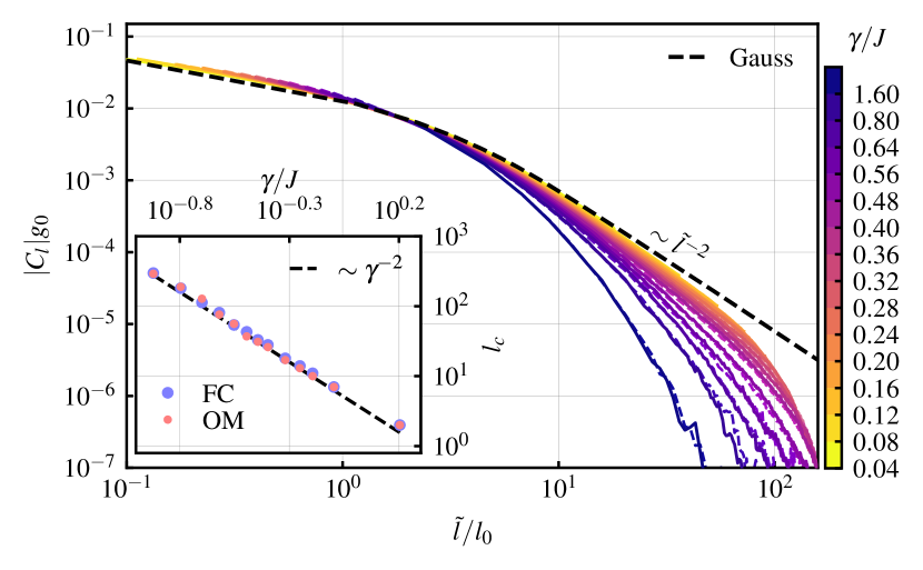
Figure 3: Rescaled density correlation function for fermion counting (solid lines) and generalized occupation measurements (colored dashed lines) for various monitoring rates $\gamma$. For $\gamma\ll J$, the data approaches the prediction from the Gaussian theory (black dashed line) with an algebraic scaling of $\sim\tilde{l}^{-2}$ for $\tilde{l}/l_{0}\gg 1$. Inset: Upper boundary of the critical range $l_{c}$ for fermion counting (FC, blue dots) and occupation measurements (OM, red dots), agreeing well with the analytical prediction $l_{c}\sim\gamma^{-2}$ (black dashed line). The system size is $L=1000$ and data are averaged over $N_{\mathrm{traj}}=160$ trajectories for this and all subsequent figures.

Figure 3 shows the density correlation function, Eq. (103), as a function of the chord length $\tilde{\ell}=\left(L/\pi\right)\sin(\pi\ell/L)$, which accounts for the finite system size and periodic boundary conditions, for both fermion counting (solid lines) and generalized occupation measurements (dashed lines). The quantitative agreement between both models despite their fundamentally different dynamics is remarkable. For comparison, we show the Gaussian result, obtained by numerically taking the inverse Fourier transform of Eq. (85) (black dashed line). The Gaussian result transitions from slow decay at short distances $\tilde{l}\ll l_{0}$ to algebraic scaling $C_{l}\sim\tilde{l}^{-2}$ on large scales $\tilde{l}\gg l_{0}$. For small values of $\gamma$, the numerical data follows the Gaussian result up to intermediate scales. However, in accord with the renormalized correlation function, Eq. (104), beyond a crossover scale $l_{c}$, the decay of the correlation function visibly becomes faster than algebraic. To quantify the deviation from the Gaussian prediction, we define $l_{c}$ as the scale beyond which the numerical data deviates from a line $\sim\tilde{l}^{-2}$, put tangentially to the data, by more than $10\,\%$. As shown in the inset of Fig. 3, the crossover scale exhibits the scaling $l_{c}\sim\gamma^{-2}$, confirming our expectation based on replica Keldysh field theory. The critical range of algebraic behavior of spatial correlations is thus bounded from below by $l_{0}$ and from above by $l_{c}$ as sketched in Fig. 1(c).

VIII.2 Entanglement entropy

We now turn to the von Neumann entanglement entropy $S_{\ell}$, Eq. (24), of a subsystem $A$ consisting of $\ell$ contiguous lattice sites. The RG flow of the NLSM indicates that area-law scaling of the entanglement entropy is established beyond the exponentially large scale $l_{*}$ in Eq. (102). However, logarithmic growth of $S_{\ell}$ as characteristic for a one-dimensional conformal field theory with central charge $c$ [83, 62],

$$S_{\ell}\sim\frac{c}{3}\ln\!\left(\ell\right),$$ (105)

can be observed within the critical range $\ell\in[l_{0},l_{c}]$.

VIII.2.1 Analytical predictions

The Gaussian theory predicts logarithmic growth of the entanglement entropy, Eq. (91), with a central charge given by $2\pi g_{0}$. To quantify the agreement of our numerical results with this prediction, we find it useful to introduce an effective scale-dependent central charge $c_{\ell}$. Equation (105) suggests to define $c_{\ell}$ as the derivative of $S_{\ell}$ with respect to $\ln(\ell)$. However, since $\ell$ is an integer, we define $c_{\ell}$ as the discrete difference,

$$c_{\ell}=3\frac{S_{\ell^{\prime}}-S_{\ell}}{\ln(\ell^{\prime}/\ell)},$$ (106)

where $\ell^{\prime}$ should be chosen such that $\ell^{\prime}/\ell=\mathrm{e}^{\epsilon}$ with $\epsilon\ll 1$. For logarithmic growth of the entanglement entropy as in Eq. (105), this definition yields $c_{\ell}=c$; volume-law scaling results in $c_{\ell}\sim\ell$, while area-law behavior leads to $c_{\ell}=0$.

To obtain an analytical prediction for $c_{\ell}$, we extend the Gaussian result, Eq. (91), by including higher orders in an asymptotic expansion in $\ell\gg l_{0}\gg 1$ and incorporating the renormalization of $g_{0}$, Eq. (101). This can be achieved by expressing the entanglement entropy $S_{\ell}$ using the cumulant expansion, Eq. (90), and Eq. (25) as

$$S_{\ell}=\frac{2\pi}{3}\int_{0}^{\infty}\frac{\mathrm{d}q}{q^{2}}C_{q}\left[1-\cos(q\ell)\right]$$ (107)

and expanding the Gaussian result for $C_{q}$, Eq. (85), to third order in $ql_{0}$. We thus obtain

$$\frac{S_{\ell}}{2\pi g_{0}/3}\sim\ln\!\left(\frac{\ell}{l_{0}}\right)+s_{0}+\frac{7l_{0}^{2}}{\ell^{2}}-\frac{1}{8\pi g_{0}}\ln\!\left(\frac{\ell}{l_{0}}\right)^{2},$$ (108)

where $s_{0}$ is a constant that does not depend on $\ell$. The first three terms on the right-hand side describe the asymptotic behavior of $S_{\ell}$ predicted by the Gaussian theory, with the leading contribution reproducing the CFT form, Eq. (105), with a central charge $c=2\pi g_{0}$. Renormalization effects are contained in the last term. The effective central charge, Eq. (106), is then

$$\frac{c_{\ell}}{2\pi g_{0}}\sim 1-\frac{14l_{0}^{2}}{\ell^{2}}-\frac{1}{4\pi g_{0}}\ln\!\left(\frac{\ell}{l_{0}}\right).$$ (109)

As explained above, $c_{\ell}\to 2\pi g_{0}$ for $\ell\gg l_{0}$ would correspond to logarithmic growth of the entanglement entropy. However, the last term in Eq. (109), which is due to the renormalization of $g_{0}$, causes the value of $c_{\ell}$ to decrease with $\ell$. Consequently, $c_{\ell}$ is never constant but only takes a maximum at

$$\ell_{\mathrm{max},c}\sim 2\sqrt{14\pi}l_{0}^{3/2}.$$ (110)

The scaling $\ell_{\mathrm{max},c}\sim l_{0}^{3/2}\sim\gamma^{-3/2}$ implies that the maximum of the effective central charge $c_{\mathrm{max}}$ is within the critical range, which is bounded from below by $l_{0}\sim\gamma^{-1}$ and from above by the crossover scale $l_{c}\sim\gamma^{-2}$. In the vicinity of the maximum, the entanglement entropy again obeys the CFT form, Eq. (105), but with $c=c_{\mathrm{max}}<2\pi g_{0}$ approaching the Gaussian result $c=2\pi g_{0}$ only for $\gamma\ll J$. It is worthwhile to reiterate that while the Gaussian theory predicts unbounded logarithmic growth of the entanglement entropy on scales $\ell\gtrsim l_{0}$ and with $c=2\pi g_{0}$, the renormalization of $g_{0}$ results in the range of logarithmic growth being restricted to $\ell\lesssim l_{c}$, and with a reduced value of the effective central charge $c_{\mathrm{max}}<2\pi g_{0}$.

VIII.2.2 Numerics

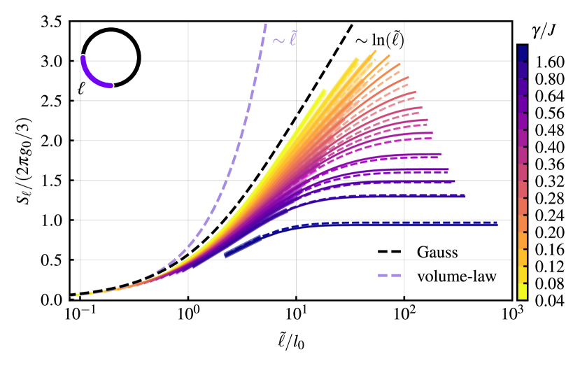
Figure 4: Rescaled entanglement entropy for fermion counting (solid lines) and generalized occupation measurements (colored dashed lines), for a subsystem of size $\ell$ of a system with periodic boundary conditions (see inset). Thicker lines indicate the extent of the critical range $\tilde{\ell}\in[l_{0},l_{c}]$. The critical range is analogously indicated in the figures below. For $\gamma\ll J$, the numerical data approach the Gaussian result obtained by inserting Eq. (85) in Eq. (107) (black dashed line), which grows logarithmically $\sim\ln(\tilde{\ell})$ for $\tilde{\ell}\gg l_{0}$. Volume-law scaling with $S_{\ell}\sim\ell$ can be observed at $\tilde{\ell}\lesssim l_{0}$ (purple dashed line).

To confirm these predictions, we have determined the entanglement entropy and effective central charge numerically. For a subsystem $A$ of size $\ell$, the entanglement entropy, Eq. (24), can be obtained from the eigenvalues $\lambda_{l}$ of the reduced single-particle density matrix $D_{A}=\left(D\right)_{l,l^{\prime}\in A}$ as [84]

$$S_{\ell}=-\sum_{l=1}^{\ell}\overline{\left[\lambda_{l}\ln(\lambda_{l})+\left(1-\lambda_{l}\right)\ln(1-\lambda_{l})\right]},$$ (111)

where the overbar again denotes an average over both trajectories and position.

Figure 4 shows the entanglement entropy for $\ell\in\{1,\dotsc,L/2\}$ for fermion counting (solid lines) and generalized occupation measurements (dashed lines). Qualitatively, these results appear to support the existence of an entanglement transition between a critical phase with logarithmic growth of the entanglement entropy and an area law phase for larger values of $\gamma$. However, an analysis of the effective central charge $c_{\ell}$ reveals clear evidence for an area-law phase for all values of $\gamma$, as predicted analytically.

Figure 5: Rescaled effective central charge calculated by applying Eq. (112) to the data shown in Fig. 4 for fermion counting (solid lines) and generalized occupation measurements (colored dashed lines). For $\gamma\ll J$, the data approach the Gaussian result (black dashed line). Upper inset: scaling of the maximum of the central charge $c_{\mathrm{max}}$ for fermion counting (blue dots) and occupation measurements (red dots) compared to the prediction obtained by inserting Eq. (110) in Eq. (109) (black dashed line). Lower inset: scaling of the position of the maximum $\ell_{\mathrm{max},c}$ of the central charge. The data agree with the predicted scaling $\sim\gamma^{-3/2}$, Eq. (110).

To account for the finite system size and periodic boundary conditions imposed in our numerical studies, we rewrite the definition of the effective scale-dependent central charge, Eq. (106), in terms of chord lengths,

$$c_{\ell}=3\frac{S_{\ell^{\prime}}-S_{\ell}}{\ln(\tilde{\ell^{\prime}}/\tilde{\ell})}.$$ (112)

Ideally, the ratio $\tilde{\ell}^{\prime}/\tilde{\ell}$ should be close to one and not depend on $\ell$. In practice, due to $\ell$ being an integer, these conditions cannot be met uniformly over the entire range of values from $\ell=1$ to $\ell=L/2$. To calculate $c_{\ell}$ numerically, we have chosen $N_{\ell}$ values $\ell_{i}$ with $\ell_{1}=1$ and $\ell_{N_{\ell}}=L/2$ such that $\tilde{\ell}^{\prime}/\tilde{\ell}=\tilde{\ell}_{i+1}/\tilde{\ell}_{i}=\mathrm{e}^{\epsilon_{i}}$ is approximately constant. For $N_{\ell}=66$, we obtain $\epsilon_{i}<0.1$ for $i>10$, ensuring that corrections to the value of $c_{\ell}$ obtained in the limit $\epsilon_{i}\to 0$ are small.

Figure 5 shows the effective central charge for fermion counting (solid lines) and generalized occupation measurements (colored dashed lines). As anticipated in Fig. 1(c), $c_{\ell}$ first grows with $\ell$, then reaches a maximum $c_{\mathrm{max}}$ at a scale $\ell_{\mathrm{max},c}$, and eventually starts to decrease, indicating the crossover to the area-law regime. The lower inset shows that the position of the maximum scales as $\ell_{\mathrm{max},c}\sim\gamma^{-3/2}$, in good agreement with Eq. (110) and within the critical range between $l_{0}\sim\gamma^{-1}$ and $l_{c}\sim\gamma^{-2}$. This finding demonstrates that the logarithmic growth of the entanglement entropy observed in Fig. 4 for small values of $\gamma$ and for $\ell\to L/2$ is due to $l_{c}$ becoming larger than $L/2$, and that the apparent transition from a critical phase to an area-law phase at larger $\gamma$ is, in fact, due to $l_{c}$ dropping below $L/2$.

Another signature of an apparent KT transition is a discontinuous jump of the central charge at a finite critical value $\gamma_{c}$ [19]. As we discuss in Sec. VIII.3 below, it is the maximum value $c_{\mathrm{max}}$ of $c_{\ell}$ that yields best agreement with CFT predictions within the critical range. The dependence of this maximum value on $\gamma$ is shown in the upper inset in Fig. 5, where we observe good agreement with the prediction obtained by inserting Eq. (110) in Eq. (109). In particular, the maximum value $c_{\mathrm{max}}$ varies smoothly with $\gamma$, providing further evidence for the absence of a KT transition at a finite $\gamma_{c}$.

VIII.3 Mutual information and conformal invariance

The scaling of the entanglement entropy, Eq. (24), with subsystem size is the key property distinguishing different measurement-induced phases. More refined measures of entanglement such as the bi- and tripartite mutual information have proven useful for locating critical points and characterizing critical phases. In particular, these quantities carry signatures of conformal invariance.

The bipartite mutual information of two disjoint subsystems $A$ and $C$, separated by a third subsystem $B$, is defined as

$$I_{2}=S_{A}+S_{C}-S_{A\cup C},$$ (113)

and provides a measure for the correlations between subsystem $A$ and $C$ [85]. In studies of measurement-induced transitions in quantum circuits, for subsystems of size $\ell_{A}=\ell_{C}=L/8$ and $\ell_{B}=3L/8$, the bipartite mutual information has been found to decay exponentially with system size $L$ in both area-law and volume-law phases [3, 5]. At the critical point, $I_{2}$ exhibits a peak that remains finite in the thermodynamic limit. Likewise, the tripartite mutual information, defined as

$$I_{3}=S_{A}+S_{B}+S_{C}+S_{A\cup B\cup C}-S_{A\cup B}-S_{B\cup C}-S_{A\cup C},$$ (114)

remains finite at the critical point [7, 86, 9]. In the area-law phase, $I_{3}$ vanishes, and it has an extensive negative value in the volume-law phase.

Apart from being indicators of measurement-induced phase transitions, the interest in the bi- and tripartite mutual information is due to the existence of analytical predictions for these quantities for one-dimensional CFTs. These predictions are expected to apply at critical points and in critical phases [19]. In CFTs, $I_{2}$ and $I_{3}$ depend only on the cross ratio [87, 88, 89],

$$x=\frac{\ell_{A}\ell_{C}}{\ell_{A\cup B}\ell_{B\cup C}}.$$ (115)

and are given by

$$\begin{split}I_{2}&=\frac{c}{3}\ln\!\left(\frac{1}{1-x}\right)+\mathcal{G}(x),\\ I_{3}&=\mathcal{G}(x),\end{split}$$ (116)

where $c$ is the central charge of the CFT and $\mathcal{G}(x)$ is a universal function that depends on the full operator content of the theory. For finite systems with periodic boundary conditions, the subsystem sizes $\ell_{A}$, $\ell_{C}$, $\ell_{A\cup B}$, and $\ell_{B\cup C}$ should be replaced by the corresponding chord lengths.

VIII.3.1 Analytical predictions

Proceeding as described in Sec. VIII.2 for the entanglement entropy, we can obtain analytical predictions for the mutual information, Eq. (113). For subsystems of size $\ell_{A}=\ell_{B}=\ell$ and $\ell_{B}=\ell^{\prime}$ with $\ell,\ell^{\prime}\gg l_{0}\gg 1$, we find

$$\frac{I_{2}}{2\pi g_{0}/3}\sim\ln\!\left(\frac{1}{1-x}\right)\left[1-\frac{\ln(\ell/l_{0})}{4\pi g_{0}}\right]-\frac{14\left(3-x\right)x^{2}l_{0}^{2}}{(x-1)^{2}\ell^{2}}.$$ (117)

For fixed cross ratio $x$ and considered as a function of $\ell$, the bipartite mutual information exhibits a maximum at

$$\ell_{\mathrm{max},I_{2}}=4\sqrt{14\pi\left(3-x\right)}\ln\!\left(\frac{1}{1-x}\right)^{-1/2}\frac{x}{\left\lvert x-1\right\rvert}l_{0}^{3/2},$$ (118)

which scales with the measurement rate as $\ell_{\mathrm{max},I_{2}}\sim\gamma^{-3/2}$, in analogy to the position of the maximum of the effective central charge given in Eq. (110).

On the same order of approximation that we have used to obtain predictions for the entanglement entropy and the bipartite mutual information, the tripartite mutual information vanishes. Indeed, generalizing Eq. (90) to $C_{A,B}^{(2)}=\sum_{l\in A,l^{\prime}\in B}C_{l-l^{\prime}}$ such that $C_{A}^{(2)}=C_{A,A}^{(2)}$, and using that the density correlation function, Eq. (76), is symmetric under the exchange of $l$ and $l^{\prime}$, we obtain $C_{A\cup B,A\cup B}^{(2)}=C_{A}^{(2)}+C_{B}^{(2)}+2C_{A,B}^{(2)}$ for any two disjoint subsystems $A$ and $B$. Then, keeping only the contribution from the second cumulant in Eq. (25), we find $I_{3}=0$, indicating that the leading contribution to the tripartite mutual information comes from the fourth cumulant. However, the fourth cumulant vanishes in a Gaussian theory. In fact, the numerical results for $I_{3}$ presented below show qualitatively different behavior for fermion counting and generalized occupation measurements. Explaining these differences analytically would require going beyond not only the Gaussian theory but even the long-wavelength effective field theory developed in Sec. VII, which is identical for both types of measurements.

VIII.3.2 Numerics

Figure 6: Rescaled bipartite mutual information for fermion counting (solid lines) and generalized occupation measurements (colored dashed lines) for subsystem sizes $\ell_{A}=\ell_{C}=\ell$ and $\ell_{B}\approx 3\ell$ (see lower inset) chosen to approximately fix the cross ratio, Eq. (115), to $x\approx 1/16$, with deviations $<1\,\%$. The Gaussian approximation is shown for comparison (black dashed line). Upper inset: scaling of the position of the maximum of the bipartite mutual information $\ell_{\mathrm{max},I_{2}}$ for fermion counting (blue dots) and occupation measurements (red dots), approaching the theoretical prediction, Eq. (118), for $\gamma\ll J$ (black dashed line). The considered subsystems are sketched in the lower left corner for periodic boundary conditions.

Figure 6 shows the bipartite mutual information for $\ell_{A}=\ell_{C}=\ell$ and $\ell_{B}\approx 3\ell$ chosen such that the cross ratio, Eq. (115), is $x\approx 1/16$ for all values of $\ell\in\{1,\dotsc,L/8\}$. The variations of $\ell_{B}/\ell\approx 3$ result in slight discontinuities in the data. Combining the finite-size phase diagram sketched in Fig. 1(c) with the known behavior of $I_{2}$ across measurement-induced phase transitions [3, 5], we expect the bipartite mutual information to be finite only within the critical range, and to decay toward zero for both $\tilde{\ell}\ll l_{0}$ and $\tilde{\ell}\gg l_{c}$. This expectation is confirmed in Fig. 6, where we find the mutual information to reach a maximum at $\ell_{\mathrm{max},I_{2}}\sim\gamma^{-3/2}$, within the critical range and in good agreement with the scaling predicted by Eq. (118).

Figure 7: Rescaled tripartite mutual information for fermion counting (solid lines) and generalized occupation measurements (colored dashed lines) for the same choice of subsystems as in Fig. 6. Volume-law behavior $\sim\tilde{\ell}$ is shown for comparison (purple dashed line). Inset: the position of the minimum of the tripartite mutual information $\ell_{\mathrm{min},I_{3}}$ scales as $\sim\gamma^{-1}$ (black dashed line) both for fermion counting (blue dots) and occupation measurements (red dots).

The tripartite mutual information is shown in Fig.7 for the same choice of subsystems as in Fig. 6. On short scales $\tilde{\ell}\lesssim l_{0}$, the tripartite mutual information behaves as expected in a volume-law phase, growing extensively to negative values for both fermion counting (solid lines) and occupation measurements (dashed lines). The minimum value of $I_{3}$ is reached at $\ell_{\mathrm{min},I_{3}}\sim\gamma^{-1}$, close to the lower boundary of the critical phase at $l_{0}\sim\gamma^{-1}$. Notably, on scales $\tilde{\ell}\gtrsim l_{0}$ beyond the volume-law regime, the tripartite mutual information shows qualitatively different behavior for fermion counting and generalized occupation measurements. For fermion counting, $I_{3}$ remains negative, and approaches $I_{3}\to 0$ from below for $\tilde{\ell}\to\infty$, as expected in an area-law phase. In contrast, for generalized occupation measurements, $I_{3}$ crosses to positive values and eventually approaches zero from above. These findings confirm that the tripartite mutual information probes behavior that is not captured by the long-wavelength effective field theory developed in Sec. VII, as discussed above.

Figure 8: Difference between bi- and tripartite mutual information for fermion counting with $\gamma/J=0.2$ (colored lines). The subsystem size $\ell_{A}=\ell_{C}=\ell$ is fixed for each curve according to the legend, while $\ell_{B}=\ell^{\prime}$ is varied to sample different values of the cross ratio $x$. For better visibility, the curves are shifted relative to each other by a factor of $2$. The CFT prediction (black dashed line) coincides with the data when $\ell^{\prime}$ is within the critical range (thicker colored lines). Violations of conformal invariance occur both on short scales $\tilde{\ell}^{\prime}\lesssim l_{0}$ (large values of $x$) and large scales $\tilde{\ell}^{\prime}\gtrsim l_{c}$ (small values of $x$).

So far, we have considered the bi- and tripartite mutual information for fixed cross ratio $x$ and as a function of subsystem size $\ell$. We now turn to a more stringent test of conformal invariance within the critical range. As we have discussed in Sec. VIII.2, on scales $\ell\gtrsim l_{0}$, the Gaussian theory predicts logarithmic growth of the entanglement entropy with a central charge $c=2\pi g_{0}$. However, due the renormalization of $g_{0}$ induced by strong fluctuations of massless replicon modes, the range of approximately logarithmic growth is actually bounded by $\ell\lesssim l_{c}$, and the value of the central charge, given by the maximum value $c_{\mathrm{max}}$ of $c_{\ell}$, is reduced as compared to the Gaussian result. These insights serve as a guideline in searching for signatures of emergent conformal symmetry in $I_{2}$ and $I_{3}$.

For a CFT, it follows from Eq. (116) that the difference $I_{2}-I_{3}$ is fully determined by the central charge and the cross ratio,

$$I_{2}-I_{3}=\frac{c}{3}\ln\!\left(\frac{1}{1-x}\right).$$ (119)

This difference is shown for fermion counting in Fig. 8. Similar results are obtained for generalized occupation measurements. A moderate value of $\gamma/J=0.2$ is chosen here to best illustrate deviations from conformal invariance at both short and large scales. Each curve corresponds to a fixed value of $\ell_{A}=\ell_{C}=\ell$, while $\ell_{B}=\ell^{\prime}$ is varied to sample different values of the cross ratio $x$, Eq. (115). We find good agreement with the CFT prediction, Eq. (119), for values $\tilde{\ell}^{\prime}\in[l_{0},l_{c}]$ within the critical range and when the central charge $c$ in Eq. (119) is set to the maximum value $c_{\mathrm{max}}$ of the effective central charge $c_{\ell}$ shown in Fig. 5. These results provide strong evidence for emergent conformal invariance within the critical range.

It should be noted that for the data shown in Fig. 8, $I_{3}$ is typically several orders of magnitude smaller than $I_{2}$. Therefore, the picture does not change when $I_{2}$ is considered instead of $I_{2}-I_{3}$. The collapse of $I_{2}$ as a function of the cross ratio for continuous measurements of occupation numbers described by a quantum state diffusion equation has been shown in Ref. [19] for a selection of subsystems. However, only the systematic analysis of the dependence on subsystem size presented above, which avoids an undersampling of subsystem sizes outside of the critical range, has allowed us to demonstrate that there is agreement with the CFT expectation only within the critical range and for $c=c_{\mathrm{max}}$.

Finally, we apply the same analysis to the tripartite mutual information. As we have already observed in Fig. 7, the tripartite mutual information exhibits qualitatively different behavior for fermion counting and occupation measurements, with $I_{3}$ assuming only negative values for fermion counting but changing sign for occupation measurements. For a CFT, Eq. (116) predicts $I_{3}$ to be a universal function of the cross ratio. Deviations from this prediction are expected in lattice systems for finite subsystem size $\ell$, and can be described by a finite-size scaling ansatz $I_{3}=\mathcal{G}(x)+\ell^{-\delta}g(x)$ [90, 91]. We do not observe a collapse of $I_{3}$ plotted as a function of the cross ratio in Fig. 9, and, at least for the data for occupation measurements shown in Fig. 9, a conventional finite-size scaling form is ruled out by the data changing sign at fixed cross ratio. As noted above, $I_{3}$ is orders of magnitude smaller than $I_{2}$. In this sense, also the violations of conformal invariance revealed by $I_{3}$ are quantitatively small. Nevertheless, it is an interesting topic for future research to understand which effects beyond the effective long-wavelength theory developed in Sec. VII determine the behavior of $I_{3}$ and cause deviations from conformal invariance within the critical range.

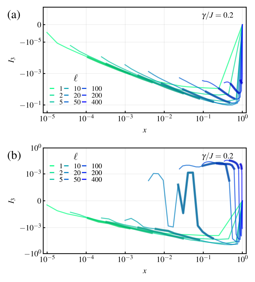
Figure 9: Tripartite mutual information as a function of the cross ratio $x$ for (a) fermion counting and (b) occupation measurements on a symmetric logarithmic scale and with $\gamma/J=0.2$. In contrast to $I_{2}-I_{3}$ shown in Fig. 8, the tripartite mutual information $I_{3}$ shows qualitatively different behavior for fermion counting and occupation measurements, and does not collapse to a single function of the cross ratio within the critical range. Fluctuations between positive and negative values of the data for occupation measurements are greatly exaggerated by the symmetric logarithmic scale.

IX Conclusions and outlook

We have presented an in-depth comparative study of two one-dimensional models of free fermions subjected to different types of generalized measurement processes: fermion counting and generalized measurements of local occupation numbers. A high rate of fermion counts signals fast fluctuations of the quantum state of the fermionic many-body system, in contrast to the freezing of the dynamics induced by frequent projective measurements or generalized measurements with measurement operators that are proportional to projectors or have a unique dark state, that is, a single state $\lvert D\rangle$ such that $\hat{M}_{n}\lvert D\rangle=0$ for all measurement operators $\hat{M}_{n}$ [92]. Despite this striking difference, the dynamics of both models have important similarities in the frequent-measurement limit: emergent classicality and a suppression of coherent dynamics, which are hallmarks of the quantum Zeno effect for occupation measurements, and which we attribute to a generalized Zeno effect for fermion counting. These similarities explain why both models exhibit close to identical results in various observables in the steady state, including density correlations, the entanglement entropy, and the bipartite mutual information. We have found qualitative differences only in the tripartite mutual information. Combining analytical insights from replica Keldysh field theory with numerical results from simulations of quantum jump trajectories, we have provided strong evidence for the absence of a measurement-induced entanglement transition in these models. In particular, we have shown that characteristic signatures of a critical phase can be observed only within a well-defined and finite range of length scales. Crucially, the upper boundary $l_{c}\sim\gamma^{-2}$ of this critical range is only algebraically large in the measurement rate, and, therefore, observable in numerics. Thus, our work contributes to clarifying the question of the existence of a measurement-induced phase transition in one-dimensional free fermions with particle number conservation.

Our work opens up several interesting directions for future research. While there is no measurement-induced phase transition in the considered models in one spatial dimension, such a transition does occur in higher dimensions [34, 38]. It will be interesting to study the impact of the breaking of particle number conservation by fermion counting on dynamical critical behavior. A classification of dynamical criticality based on symmetries and conservation laws—in analogy to the classification of dynamical criticality in thermodynamic equilibrium [93]—is an interesting prospect. However, exploring this possibility analytically by studying, for example, two-time correlation functions such as $\overline{\left\langle\hat{A}(t)\right\rangle\left\langle\hat{B}(t^{\prime})\right\rangle}$ will require a nontrivial extension of the replica Keldysh formalism.

From a more formal perspective, the stochastic Schrödinger equation (3) can be regarded as an unravelling of a quantum master equation that is recovered by taking the average over the stochastic increments $\mathrm{d}N_{\alpha,l}(t)$. While here we have considered cases for which the stationary state of the unconditional dynamics described by the master equation is trivial, this is generically not the case, and jump operators can be chosen so as to prepare a state of interest. For example, consider a one-dimensional fermionic chain that is connected to particle reservoirs only at its ends and in such a way that a finite current is driven through the system. An unravelling of the corresponding master equation represents an interesting setup to study the interplay of transport and entanglement dynamics on the level of individual quantum trajectories. However, such an unravelling can, in general, not be formulated as a random generalized measurement, and the derivation of a replica Keldysh field theory described in Sec. V has to be modified.

Finally, it is an interesting perspective to investigate quantum jump unravellings of quadratic fermionic Liouvillians belonging to different symmetry classes [94, 95, 96, 97]. The resulting replica Keldysh field theories and NLSMs will shed further light on the connections between the dynamics of continuously monitored quantum systems in $d$ spatial dimensions and the physics of Anderson localization in $d+1$ dimensions [98].

Appendix A Minimal physical models and their description through a stochastic Schrödinger equation

In this appendix, we outline the derivation of the stochastic Schrödinger equation (3) for minimal physical models of fermion counting and generalized occupation measurements.

A.1 Fermion counting

We consider the setup of a quantum dot coupled to two reservoirs described in Sec. III.1 [60]. The quantum dot corresponds to a single fermionic lattice site, with annihilation and creation operators $\hat{\psi}$ and $\hat{\psi}^{\dagger}$, respectively, and Hamiltonian

$$\hat{H}_{0}=\omega_{0}\hat{\psi}^{\dagger}\hat{\psi}.$$ (120)

We denote the reservoir annihilation and creation operators by $\hat{b}_{\alpha,k}$ and $\hat{b}_{\alpha,k}^{\dagger}$, where $\alpha=-$ for the reservoir that acts as the drain, $\alpha=+$ for the reservoir that acts as the source, and $k$ is a discrete index that labels the reservoir modes. The Hamiltonians of the reservoirs modes with energies $\omega_{\alpha,k}$ read

$$\hat{H}_{\alpha}=\sum_{k}\omega_{\alpha,k}\hat{b}_{\alpha,k}^{\dagger}\hat{b}_{\alpha,k},$$ (121)

and the reservoirs are coupled to the quantum dot by

$$\hat{H}_{\mathrm{coup}}=\mathrm{i}\sum_{\alpha,k}\left(T_{\alpha,k}\hat{\psi}^{\dagger}\hat{b}_{\alpha,k}-T_{\alpha,k}^{\ast}\hat{b}_{\alpha,k}^{\dagger}\hat{\psi}\right),$$ (122)

with tunneling coefficients $T_{\alpha,k}$. Both reservoirs are assumed to be in thermodynamic equilibrium at a low temperature, with chemical potentials chosen such that the reservoir modes at the energy $\omega_{0}$ are empty in the drain and occupied in the source. We model this scenario by assuming the dot and reservoirs to be in the pure state $\lvert\Psi(0)\rangle=\lvert\psi(0)\rangle\otimes\lvert 0_{-}\rangle\otimes\lvert 1_{+}\rangle$ at time $t=0$, with $\lvert 0_{-}\rangle$ and $\lvert 1_{+}\rangle$ denoting empty and occupied states of the drain and source, respectively.

Our goal is to derive a stochastic Schrödinger equation describing the dynamics of the quantum dot. As a first step, we move to an interaction frame with respect to the bath Hamiltonians, Eq. (121), and integrate the Schrödinger equation for the state $\lvert\Psi(t)\rangle$ of the dot and reservoirs in small time steps $\Delta t$. In Born and Markov approximations, the increment of the wave function, $\Delta\lvert\Psi(t)\rangle=\lvert\Psi(t+\Delta t)\rangle-\lvert\Psi(t)\rangle$, is given by [99]

$$\Delta\lvert\Psi(t)\rangle=\left[-\mathrm{i}\hat{H}_{\mathrm{eff}}\Delta t+\sqrt{2}\hat{L}_{-}\Delta\hat{B}_{-}^{\dagger}(t)+\sqrt{2}\hat{L}_{+}\Delta\hat{B}_{+}(t)\right]\lvert\Psi(t)\rangle.$$ (123)

The effective Hamiltonian reads

$$\hat{H}_{\mathrm{eff}}=\hat{H}_{0}-\mathrm{i}\sum_{\alpha=\pm}\hat{L}_{\alpha}^{\dagger}\hat{L}_{\alpha},$$ (124)

where $\hat{L}_{-}=\sqrt{\gamma_{-}/2}\,\hat{\psi}$ and $\hat{L}_{+}=\sqrt{\gamma_{+}/2}\,\hat{\psi}^{\dagger}$ are the jump operators defined in Eq. (4) for a single lattice site. Further, in Eq. (123), we have introduced quantum Itô increments,

$$\Delta\hat{B}_{\alpha}(t)=\sqrt{\frac{2}{\gamma_{\alpha}}}\int_{t}^{t+\Delta t}\mathrm{d}t^{\prime}\sum_{k}T_{\alpha,k}\hat{b}_{\alpha,k}\mathrm{e}^{-\mathrm{i}\omega_{\alpha,k}t^{\prime}},$$ (125)

which obey the anticommutation relations

$$\left\{\Delta\hat{B}_{\alpha}^{\vphantom{\dagger}}(t),\Delta\hat{B}_{\alpha}^{\dagger}(t^{\prime})\right\}=\Delta t\,\delta_{t,t^{\prime}}^{\vphantom{\dagger}},$$ (126)

where $\delta_{t,t^{\prime}}$ is the Kronecker delta for discrete times $t$ and $t^{\prime}$. Finally, the loss and gain rates appearing in Eq. (123) are defined as $\gamma_{\alpha}=2\pi\rho_{\pm}(\omega_{0})\left\lvert T_{\pm}(\omega_{0})\right\rvert$, where $\rho_{\alpha}(\omega_{0})$ and $T_{\alpha}(\omega_{0})$ are the density of states and tunneling amplitudes at the energy of the dot, which are introduced upon taking the continuum limit such that $\sum_{k}\to\int_{0}^{\infty}\mathrm{d}\omega\,\rho_{\alpha}(\omega)$ and $T_{\alpha,k}\to T_{\alpha}(\omega)$ [60].

The operators $\hat{L}_{-}\Delta\hat{B}_{-}^{\dagger}(t)$ and $\hat{L}_{+}\Delta\hat{B}_{+}(t)$ in Eq. (123) describe the transfer of a fermion from the quantum dot to the drain and from the source to the dot, respectively. Since the Itô increments anticommute at different times, a fermion that has been transferred from the dot to the drain at time $t$ cannot be transferred back at a later time $t^{\prime}$. Formally, the state $\Delta\hat{B}_{-}^{\dagger}(t)\lvert 0_{-}\rangle$ is annihilated by $\Delta\hat{B}_{-}(t^{\prime})$. An analogous argument applies to the transfer of fermions from the source to the dot. Therefore, in Eq. (123), the operators $\Delta\hat{B}_{-}(t)$ and $\Delta\hat{B}_{+}^{\dagger}(t)$ do not occur.

In analogy to photon counting in quantum optics, fermion counting is implemented by measuring the number operators,

$$\hat{N}_{\alpha}(t)=\frac{\Delta\hat{B}_{\alpha}^{\dagger}(t)}{\sqrt{\Delta t}}\frac{\Delta\hat{B}_{\alpha}(t)}{\sqrt{\Delta t}},$$ (127)

at each time step, with possible measurement outcomes $N_{\alpha}(t)=0,1$. To describe the statistics of the measurement outcomes and the change of the state of the quantum dot for a given outcome, it is convenient to rewrite Eq. (123) in the form

$$\lvert\Psi(t+\Delta t)\rangle=\left[\hat{M}_{0}+\hat{M}_{-}\frac{\Delta\hat{B}_{-}^{\dagger}(t)}{\sqrt{\Delta t}}+\hat{M}_{+}\frac{\Delta\hat{B}_{+}(t)}{\sqrt{\Delta t}}\right]\lvert\Psi(t)\rangle,$$ (128)

where the measurement operators are defined as

$$\hat{M}_{0}=1-\mathrm{i}\hat{H}_{\mathrm{eff}}\Delta t,\quad\hat{M}_{-}=\sqrt{2\Delta t}\,\hat{L}_{-},\quad\hat{M}_{+}=\sqrt{2\Delta t}\,\hat{L}_{+}.$$ (129)

A measurement of the number operators, Eq. (127), performed on the state $\lvert\Psi(t+\Delta t)\rangle$, Eq. (128), yields $N_{-}(t)=0$ and $N_{+}(t)=1$ with probability

$$p_{0}(t)=\left\langle\psi(t)\middle|\hat{M}_{0}^{\dagger}\hat{M}_{0}\middle|\psi(t)\right\rangle.$$ (130)

After a measurement with this outcome, the state of the quantum dot is given by

$$\lvert\psi(t+\Delta t)\rangle=\frac{\hat{M}_{0}\lvert\psi(t)\rangle}{\sqrt{p_{0}(t)}}=\left[1-\mathrm{i}\hat{H}_{\mathrm{eff}}\Delta t+\sum_{\alpha=\pm}\tilde{p}_{\alpha}(t)\Delta t\right]\lvert\psi(t)\rangle,$$ (131)

where we have expanded the denominator up to order $\Delta t$, and where, as in Eq. (5), we have defined

$$\tilde{p}_{\alpha}(t)=\left\langle\psi(t)\middle|\hat{L}_{\alpha}^{\dagger}\hat{L}_{\alpha}\middle|\psi(t)\right\rangle.$$ (132)

The measurement outcome above and the change of the state in Eq. (131) correspond to the case that no quantum jump has occurred during the time step, and the states of drain and source remain unchanged. In contrast, for $N_{-}(t)=1$ and $N_{+}(t)=1$, one fermion has been transferred from the quantum dot to the drain. This happens with probability $p_{-}(t)=2\tilde{p}_{-}(t)\Delta t$, and the state after the measurement is

$$\lvert\psi(t+\Delta t)\rangle=\frac{\hat{M}_{-}\lvert\psi(t)\rangle}{\sqrt{p_{-}(t)}}=\frac{\hat{L}_{-}\lvert\psi(t)\rangle}{\sqrt{\tilde{p}_{-}(t)}}.$$ (133)

For $N_{-}(t)=0$ and $N_{+}(t)=0$, a fermion has been transferred from the source to the dot, which happens with probability $p_{+}(t)=2\tilde{p}_{+}(t)\Delta t$. Then, the state after the measurement is

$$\lvert\psi(t+\Delta t)\rangle=\frac{\hat{M}_{+}\lvert\psi(t)\rangle}{\sqrt{p_{+}(t)}}=\frac{\hat{L}_{+}\lvert\psi(t)\rangle}{\sqrt{\tilde{p}_{+}(t)}}.$$ (134)

Performing measurements of the number operators, Eq. (127), in each time step results in stochastic dynamics of the wave function of the quantum dot, conditional to the measurement outcomes. To formulate these dynamics as an evolution equation, we define stochastic increments $\Delta N_{\alpha}(t)=0,1$ that count the number of fermions that are transferred from the dot to the drain and from the source to the dot during the step from $t$ to $t+\Delta t$. Neglecting terms of order $\Delta N_{\alpha}(t)\Delta t$ [60], we can thus write the increment of the wave function as

$$\Delta\lvert\psi(t)\rangle=\left\{\left[-\mathrm{i}\hat{H}_{\mathrm{eff}}+\sum_{\alpha=\pm}\tilde{p}_{\alpha}(t)\right]\Delta t\right.\\ \left.+\sum_{\alpha=\pm}\left[\frac{\hat{L}_{\alpha}}{\sqrt{\tilde{p}_{\alpha}(t)}}-1\right]\Delta N_{\alpha}(t)\right\}\lvert\psi(t)\rangle.$$ (135)

In the limit of infinitesimal time steps, $\Delta t\to\mathrm{d}t$, the stochastic increments $\Delta N_{\alpha}(t)\to\mathrm{d}N_{\alpha}(t)$ describe a Poisson point process with the properties specified in Sec. III.1 [100], and the evolution of the quantum dot is then described by the stochastic Schrödinger equation (3) with $L=1$ and where we omit the contribution from $\hat{H}_{0}$, Eq. (120), which leads to a global phase factor for each trajectory.

A.2 Generalized occupation measurements

Measurements of the occupation of a quantum dot can be implemented by modifying the above setup as outlined in Sec. III.1: Instead of tunneling from the reservoirs to the dot as described by Eq. (122), we consider tunneling directly from the source to the drain which, however, is possible only when the dot is occupied [60],

$$\hat{H}_{\mathrm{coup}}=\mathrm{i}\sum_{k,q}\hat{\psi}^{\dagger}\hat{\psi}\left(\chi\hat{b}_{-,k}^{\dagger}\hat{b}_{+,q}+\chi^{\ast}\hat{b}_{+,q}^{\dagger}\hat{b}_{-,k}\right).$$ (136)

This coupling Hamiltonian, with a mode-independent tunneling rate $\chi$, is a simplified version of a setup that has been realized in mesoscopic devices, for example, in Ref. [64].

As above, we integrate the Schrödinger equation for the dot and reservoirs in small time steps, leading to

$$\Delta\lvert\Psi(t)\rangle=\left[-\mathrm{i}\hat{H}_{\mathrm{eff}}\Delta t+\sqrt{2}\hat{L}\Delta\hat{B}(t)\right]\lvert\Psi(t)\rangle,$$ (137)

where $\hat{n}=\hat{\psi}^{\dagger}\hat{\psi}$ and $\hat{L}=\sqrt{\gamma}\,\hat{n}$. The measurement rate is $\gamma=2\pi\rho_{-}(\omega_{0})\rho_{+}(\omega_{0})\left\lvert\chi\right\rvert^{2}\left(\mu_{+}-\mu_{-}\right)$, where $\mu_{\alpha}$ are the chemical potentials of the reservoirs, and the effective Hamiltonian is given by

$$\hat{H}_{\mathrm{eff}}=\hat{H}_{0}-\mathrm{i}\hat{L}^{\dagger}\hat{L}.$$ (138)

We have again introduced quantum Itô increments,

$$\Delta\hat{B}(t)=\sqrt{\frac{\gamma}{2}}\chi^{*}\int_{t}^{t+\Delta t}\mathrm{d}t^{\prime}\sum_{k,q}\hat{b}_{-,k}^{\dagger}\hat{b}_{+,q}\mathrm{e}^{-\mathrm{i}\left(\omega_{+,q}-\omega_{-,k}\right)t^{\prime}}.$$ (139)

which obey canonical anticommutation relations,

$$\left\{\Delta\hat{B}(t),\Delta\hat{B}^{\dagger}(t^{\prime})\right\}=\Delta t\,\delta_{t,t^{\prime}}.$$ (140)

From here on, the derivation of the stochastic Schrödinger equation describing the dynamics of the quantum dot is analogous to the one for fermion counting outlined above.

Appendix B Regularization, causality structure, and normalization in Keldysh field theory

Here, we address points (i) and (ii) listed below Eq. (46). Further, we discuss the causality structure and normalization of the Keldysh partition function in the replica limit $R\to 1$.

B.1 Regularization of the Keldysh action

(i) In the construction of the Keldysh functional integral, in Eq. (36), time evolution from $t_{0}$ to $t$ is split into $N$ time steps of duration $\Delta t=(t-t_{0})/N$. At each discrete time $t_{n}=t_{0}+\Delta tn$, a resolution of the identity in terms of coherent states, $\lvert\pm\psi_{\pm,n}\rangle=\mathrm{e}^{\pm\sum_{r=1}^{R}\sum_{l=1}^{L}\psi_{\pm,r,l,n}\hat{\psi}_{r,l}^{\dagger}}\lvert\Omega\rangle$, where $\lvert\Omega\rangle$ is the vacuum state, is inserted. If a measurement is performed between times $t_{n}$ and $t_{n+1}$, we thus obtain a matrix element of the measurement operator between the coherent states $\lvert\psi_{\pm,n}\rangle$ and $\lvert\psi_{\pm,n+1}\rangle$. For generalized occupation measurements with measurement operators given in Eq. (16), the matrix elements on the forward and backward branches contain the factors

$$\begin{split}\left\langle\psi_{+,n+1}|\hat{n}_{r,l}|\psi_{+,n}\right\rangle&=\bar{\psi}_{+,r,l,n+1}\psi_{+,r,l,n}\left\langle\psi_{+,n+1}|\psi_{+,n}\right\rangle,\\ \left\langle-\psi_{-,n}|\hat{n}_{r,l}|-\psi_{-,n+1}\right\rangle&=\bar{\psi}_{-,r,l,n}\psi_{-,r,n+1,l}\left\langle-\psi_{-,n}|-\psi_{-,n+1}\right\rangle,\end{split}$$ (141)

where the fields that represent the operators $\hat{n}_{r,l}$ are one discrete time step apart. However, as shown in Ref. [30], in the functional integral, we can replace

$$\begin{split}\bar{\psi}_{+,r,l,n+1}\psi_{+,r,l,n}&\to\bar{\psi}_{+,r,l,n}\psi_{+,r,l,n}+1,\\ \bar{\psi}_{-,r,l,n}\psi_{-,r,l,n+1}&\to\bar{\psi}_{-,r,l,n}\psi_{-,r,l,n}+1,\end{split}$$ (142)

where now the fields are evaluated at equal times. This is a prerequisite for introducing fermionic bilinears at equal times as new variables. The vertex in Eq. (44) is thus modified as

$$V[\bar{\psi}_{r},\psi_{r}]=\frac{1}{n}\left(\bar{\psi}_{+,r}\psi_{+,r}+1\right)\left(\bar{\psi}_{-,r}\psi_{-,r}+1\right).$$ (143)

For fermion counting, with the linear measurement operators in Eq. (15), this issue does not arise.

(ii) In the discrete-time formulation of the theory, the Green’s function is defined as $\mathrm{i}G_{n,n^{\prime}}=\left\langle\psi_{n}\bar{\psi}_{n^{\prime}}\right\rangle$ [78]. Working in the basis introduced through the Larkin-Ovchinnikov rotation, Eq. (45), the continuous-time limit is given by

$$G(t,t^{\prime})=\lim_{n,n^{\prime},N\to\infty}\left(G_{n,n^{\prime}}+\frac{\mathrm{i}}{2}\delta_{n,n^{\prime}}\sigma_{x}\right),$$ (144)

where the limit is taken such that $t_{n}\to t$ and $t_{n^{\prime}}\to t^{\prime}$. In the last term, we leave the identity matrices in replica and lattice space implicit. The shift $\mathrm{i}\delta_{n,n^{\prime}}\sigma_{x}/2$ on the right-hand side leads to the continuous-time Green’s function at equal times being given by the symmetrized limit as in Eq. (46),

$$G(t,t)=\frac{1}{2}\left[G(t,t+0^{+})+G(t,t-0^{+})\right].$$ (145)

In turn, this implies that the Keldysh Green’s function is continuous at $t=t^{\prime}$, and that the anti-Keldysh component of the Green’s function vanishes at all times—which is not the case for the discrete-time Green’s function $G_{n,n^{\prime}}$ that has a nonvanishing anti-Keldysh component at $n=n^{\prime}$ [78].

For most applications of Keldysh field theory, the shift on the right-hand side of Eq. (144) is irrelevant and can be omitted. However, here we have to take it into account to ensure normalization of the Keldysh partition function as discussed below. The shift can be incorporated in the action by switching to a regularization in which the free discrete-time Green’s function is $G^{\mathrm{(reg)}}_{n,n^{\prime}}=G_{n,n^{\prime}}+\mathrm{i}\delta_{n,n^{\prime}}\sigma_{x}/2$ [58]. Changing the regularization is achieved through the following relation:

$$\begin{split}Z_{R}(t)&=\int\frac{\mathrm{D}[\bar{\psi},\psi]}{\mathop{\mathrm{Det}}\!\left(-\mathrm{i}G_{0}^{-1}\right)}\,\mathrm{e}^{\mathrm{i}\left(\bar{\psi}G_{0}^{-1}\psi+\gamma\int\mathrm{d}^{2}\mathbf{x}\,\mathcal{L}_{M}[\bar{\psi}_{l},\psi_{l}]\right)}\\ &=\int\frac{\mathrm{D}[\bar{\psi},\psi]}{\mathop{\mathrm{Det}}\!\left(-\mathrm{i}G_{0}^{\mathrm{(reg)}-1}\right)}\,\mathrm{e}^{\mathrm{i}\left(\bar{\psi}G_{0}^{\mathrm{(reg)}-1}\psi+\gamma\int\mathrm{d}^{2}\mathbf{x}\,\mathcal{L}_{M}^{\mathrm{(reg)}}[\bar{\psi}_{l},\psi_{l}]\right)},\end{split}$$ (146)

where we make the determinants that are usually absorbed in the integration measure explicit [78]. The regularized measurement Lagrangian can be constructed order by order in an expansion in $\gamma$. To first order, $\mathcal{L}_{M}^{\mathrm{(reg)}}$ is obtained by adding the sum over all partial contractions, where each contraction is $\left\langle\psi_{n}\bar{\psi}_{n^{\prime}}\right\rangle=\delta_{n,n^{\prime}}\sigma_{x}/2$, to the original measurement Lagrangian $\mathcal{L}_{M}$. Since these contractions are diagonal in replica space, they can be added to each factor of the product over replicas in Eq. (42), that is, to the vertices Eqs. (43) and (143). As stated in the main text, the vertices for fermion counting do not change under the regularization. The regularized vertex for occupation measurements is given in Eq. (48).

B.2 Causality structure and normalization of the Keldysh partition function

For closed quantum systems undergoing unitary dynamics without measurements, the Keldysh partition function is normalized to unity, $Z(t)=\mathop{\mathrm{tr}}(\hat{\rho}(t))=1$, as follows from the normalization of the density matrix $\hat{\rho}(t)$. However, the replica Keldysh partition function $Z_{R}(t)$ is defined in Eq. (36) in terms of $R$ copies of the nonnormalized density matrix $\hat{D}(t)$. In the replica limit $R\to 1$, the completeness relation of measurement operators implies again that $Z_{R}(t)\to 1$. For $R>1$, on the other hand, the replica Keldysh partition function is not normalized. This is because the products of measurement operators over $r$ replicas, which occur in $\otimes_{r=1}^{R}\hat{D}_{r}(t)$, do not obey a completeness relation.

In Keldysh field theory for closed systems, the normalization of the partition function is reflected in the causality structure of the action, in particular, in the property that the action vanishes for $\psi_{+}=\psi_{-}$ and $\bar{\psi}_{+}=\bar{\psi}_{-}$ [77, 78, 79, 80]. To see this, we consider a system with Hamiltonian $\hat{H}$. The Keldysh partition function is $Z(t)=\int\mathrm{D}[\bar{\psi},\psi]\,\mathrm{e}^{\mathrm{i}S}$ where $S=\int_{t_{0}}^{t}\mathrm{d}t^{\prime}\mathcal{L}[\bar{\psi},\psi]$, and with the Lagrangian

$$\mathcal{L}[\bar{\psi},\psi]=\sum_{\sigma=\pm}\sigma\left(\bar{\psi}_{\sigma}\partial_{t}\psi_{\sigma}-H[\bar{\psi}_{\sigma},\psi_{\sigma}]\right).$$ (147)

From $Z(t)=\mathop{\mathrm{tr}}(\hat{\rho}(t))=1$ it follows that

$$\partial_{t}Z=\mathrm{i}\left\langle\mathcal{L}[\bar{\psi},\psi]\right\rangle=\mathrm{i}\sum_{\sigma=\pm}\sigma\left\langle\bar{\psi}_{\sigma}\partial_{t}\psi_{\sigma}-H[\bar{\psi}_{\sigma},\psi_{\sigma}]\right\rangle=0.$$ (148)

Upon taking the sum over $\sigma=\pm$, both terms in the average vanish individually. Indeed, the cyclic property of the trace implies that the expectation value of any operator $\hat{O}$ at time $t$ can be evaluated equivalently on the forward and on the backward branch of the Keldysh contour, and, therefore,

$$\left\langle\mathcal{L}[\bar{\psi},\psi]\right\rangle=\left\langle\left.\mathcal{L}[\bar{\psi},\psi]\right.\rvert_{\psi_{+}=\psi_{-},\bar{\psi}_{+}=\bar{\psi}_{-}}\right\rangle.$$ (149)

Then, $\left\langle\mathcal{L}[\bar{\psi},\psi]\right\rangle=0$ follows for the Lagrangian of a closed system in Eq. (147) from the causality structure,

$$\left.\mathcal{L}[\bar{\psi},\psi]\right.\rvert_{\psi_{+}=\psi_{-},\bar{\psi}_{+}=\bar{\psi}_{-}}=0.$$ (150)

This shows that the causality structure of the action guarantees the normalization of the Keldysh partition function.

As mentioned in Sec. V.2, the term $\bar{\psi}_{2}\psi_{1}$ in the regularized vertex for occupation measurements, Eq. (48), violates the usual causality structure. Inverting the Larkin-Ovchinnikov rotation, Eq. (45), shows that this term couples the forward and backward branches. The above argument based on the cyclic property of the trace does, in general, not apply, and Eqs. (149) and (150) do not hold for such terms. To see that the partition function is normalized even though the action does not obey the usual causality structure, one should note that according to Eq. (148), normalization is ensured when the expectation value of the Lagrangian vanishes. We will now confirm that this condition is met.

The free evolution described by the first term in the Keldysh action in Eq. (41) obeys the causality structure for any value of $R$, and, therefore, we only need to consider the measurement Lagrangian Eq. (42). For $R=1$, we thus require

$$\left\langle\mathrm{i}\mathcal{L}_{M}[\bar{\psi},\psi]\right\rangle=\sum_{n=\pm}\left\langle V_{n}[\bar{\psi},\psi]\right\rangle-1=0.$$ (151)

We first check this condition for fermion counting. Using the form of the vertices given in Eq. (47), we obtain

$$\left\langle\mathrm{i}\mathcal{L}_{M}[\bar{\psi}_{l},\psi_{l}]\right\rangle=\mathrm{i}\left[G_{l,l}^{R}(t,t)-G_{l,l}^{A}(t,t)\right]-1.$$ (152)

To evaluate the Green’s functions at equal times, we express them through fermionic field operators [77]:

$$\begin{split}\mathrm{i}G_{l,l^{\prime}}^{R}(t,t^{\prime})&=\left\langle\psi_{1,l}(t)\bar{\psi}_{1,l^{\prime}}^{*}(t^{\prime})\right\rangle=\theta(t-t^{\prime})\left\langle\left\{\hat{\psi}_{l}(t),\hat{\psi}_{l^{\prime}}^{\dagger}(t^{\prime})\right\}\right\rangle,\\ \mathrm{i}G^{A}_{l,l^{\prime}}(t,t^{\prime})&=\left\langle\psi_{2,l}(t)\bar{\psi}_{2,l^{\prime}}^{*}(t^{\prime})\right\rangle=-\theta(t^{\prime}-t)\left\langle\left\{\hat{\psi}_{l}(t),\hat{\psi}_{l^{\prime}}^{\dagger}(t^{\prime})\right\}\right\rangle,\\ \mathrm{i}G_{l,l^{\prime}}^{K}(t,t^{\prime})&=\left\langle\psi_{1,l}(t)\bar{\psi}_{2,l^{\prime}}^{*}(t^{\prime})\right\rangle=\left\langle\left[\hat{\psi}_{l}(t),\hat{\psi}_{l^{\prime}}^{\dagger}(t^{\prime})\right]\right\rangle,\end{split}$$ (153)

where two-time averages are defined as in Eq. (20). The values of the Green’s functions in the symmetrized limit of equal times, Eq. (145), follow directly from fermionic anticommutation relations and the expectation value $\left\langle\hat{n}_{l}\right\rangle_{\mathrm{ss}}$ in the unconditional steady state. According to Sec. III.1, $\left\langle\hat{n}_{l}\right\rangle_{\mathrm{ss}}=n$ for occupation measurements, with $n=1/2$ for fermion counting with equal rates of loss and gain. We thus obtain

$$\mathrm{i}G_{l,l^{\prime}}^{R/A}(t,t)=\pm\frac{1}{2}\delta_{l,l^{\prime}},\quad\mathrm{i}G_{l,l^{\prime}}^{K}(t,t)=\left(1-2n\right)\delta_{l,l^{\prime}}.$$ (154)

Inserting these values in Eq. (152) yields $\left\langle\mathrm{i}\mathcal{L}_{M}[\bar{\psi}_{l},\psi_{l}]\right\rangle=0$, confirming that the Keldysh partition function is normalized.

Finally, we check Eq. (151) for occupation measurements. Since the regularized vertex Eq. (48) is quartic, the expectation value in Eq. (151) cannot be evaluated exactly. At lowest order in $\gamma$, we can use Wick’s theorem to obtain

$$\left\langle\mathrm{i}\mathcal{L}_{M}[\bar{\psi}_{l},\psi_{l}]\right\rangle=\frac{1}{n}\left[\frac{1}{4}-\frac{\mathrm{i}}{2}G^{K}_{l,l}(t,t)+G^{R}_{l,l}(t,t)G^{A}_{l,l}(t,t)\right]-1,$$ (155)

where now the Green’s functions are those of the system without measurements. However, Eq. (154) still applies, and we again find $\left\langle\mathrm{i}\mathcal{L}_{M}[\bar{\psi}_{l},\psi_{l}]\right\rangle=0$.

Appendix C Symmetry of the measurement Lagrangian under $\mathcal{R}_{\Phi}$

Rotations of the form $\mathcal{R}_{\Phi}=\mathrm{e}^{\mathrm{i}\Phi\sigma_{x}/2}$ with a traceless Hermitian matrix $\Phi$ are a symmetry of the measurement Lagrangian for fermion counting, Eq. (51). To prove this statement, we first perform two auxiliary calculations. We define the adjoint action of a matrix $A$ on a matrix $B$ as $\mathcal{A}_{A}B=\left[A,B\right]$. Then,

$$\begin{split}\mathcal{R}_{\Phi}^{-1}\tau_{\pm}\mathcal{R}_{\Phi}&=\sum_{n=0}^{\infty}\frac{\left(-\mathrm{i}\right)^{n}}{n!}\mathcal{A}_{\Phi\sigma_{x}/2}^{n}\tau_{\pm}=\sum_{n=0}^{\infty}\frac{\left(\mp\mathrm{i}\Phi\right)^{n}}{n!}\tau_{\pm}=\tau_{\pm}\mathrm{e}^{\mp\mathrm{i}\Phi},\end{split}$$ (156)

where we have used that $\tau_{\pm}$ is invariant—up to a change of sign—under multiplication by $\sigma_{x}$ from both the left and the right, $\sigma_{x}\tau_{\pm}=\pm\tau_{\pm}$ and $\tau_{\pm}\sigma_{x}=\mp\tau_{\pm}$, which can be combined to $\mathcal{A}_{\sigma_{x}}\tau_{\pm}=\pm 2\tau_{\pm}$. Next, for a matrix $A$ in Keldysh and replica space, we consider

$$\mathop{\mathrm{tr}_{K}}\!\left(\mathcal{R}_{\Phi}\tau_{\pm}A\mathcal{R}_{\Phi}^{-1}\right)\\ \begin{aligned} &=\sum_{n=0}^{\infty}\frac{\mathrm{i}^{n}}{n!}\mathop{\mathrm{tr}_{K}}\!\left(\mathcal{A}_{\Phi\sigma_{x}/2}^{n}\tau_{\pm}A\right)=\sum_{n=0}^{\infty}\frac{\mathrm{i}^{n}}{n!}\mathcal{A}_{\Phi/2}^{n}\mathop{\mathrm{tr}_{K}}\!\left(\sigma_{x}^{n}\tau_{\pm}A\right)\\ &=\sum_{n=0}^{\infty}\frac{\left(\pm\mathrm{i}\right)^{n}}{n!}\mathcal{A}_{\Phi/2}^{n}\mathop{\mathrm{tr}_{K}}\!\left(\tau_{\pm}A\right)=\mathrm{e}^{\pm\mathrm{i}\Phi/2}\mathop{\mathrm{tr}_{K}}(\tau_{\pm}A)\mathrm{e}^{\mp\mathrm{i}\Phi/2},\end{aligned}$$ (157)

These two results and $\mathop{\mathrm{det}_{R}}\!\left(\mathrm{e}^{\mp\mathrm{i}\Phi}\right)=\mathrm{e}^{\mp\mathrm{i}\mathop{\mathrm{tr}_{R}}(\Phi)}=1$ lead to

$$\mathop{\mathrm{det}_{R}}\!\left[\mathop{\mathrm{tr}_{K}}\!\left(\tau_{\pm}\mathcal{R}_{\Phi}\mathcal{G}\mathcal{R}_{\Phi}^{-1}\right)\right]=\mathop{\mathrm{det}_{R}}\!\left[\mathop{\mathrm{tr}_{K}}\!\left(\mathcal{R}_{\Phi}\tau_{\pm}\mathrm{e}^{\mp\mathrm{i}\Phi}\mathcal{G}\mathcal{R}_{\Phi}^{-1}\right)\right]\\ \begin{aligned} &=\mathop{\mathrm{det}_{R}}\!\left[\mathrm{e}^{\pm\mathrm{i}\Phi/2}\mathop{\mathrm{tr}_{K}}\!\left(\tau_{\pm}\mathrm{e}^{\mp\mathrm{i}\Phi}\mathcal{G}\right)\mathrm{e}^{\mp\mathrm{i}\Phi/2}\right]\\ &=\mathop{\mathrm{det}_{R}}\!\left(\mathrm{e}^{\mp\mathrm{i}\Phi}\right)\mathop{\mathrm{det}_{R}}\!\left[\mathop{\mathrm{tr}_{K}}\!\left(\tau_{\pm}\mathcal{G}\right)\right]=\mathop{\mathrm{det}_{R}}\!\left[\mathop{\mathrm{tr}_{K}}\!\left(\tau_{\pm}\mathcal{G}\right)\right],\end{aligned}$$ (158)

showing that the transformation $\mathcal{G}\mapsto\mathcal{R}_{\Phi}\mathcal{G}\mathcal{R}_{\Phi}^{-1}$ is indeed a symmetry of Eq. (51) for $R>1$.

The above derivation relies on $\tau_{\pm}$ being invariant under multiplication by $\sigma_{x}$. This invariance does not apply to multiplication by $\sigma_{y}$ or $\sigma_{z}$. Therefore, rotations with $\sigma_{x}$ replaced by $\sigma_{y}$ or $\sigma_{z}$ are not symmetries of the measurement Lagrangian.

Appendix D Fluctuation expansion of the Keldysh action

To obtain the variation of the Keldysh action with respect to $\mathcal{G}$ and thereby find the saddle-point manifolds described by Eqs. (64) and (65), and to derive the action that governs the Gaussian theory discussed in Sec. VI, we perform an expansion of the Keldysh action around its saddle points.

D.1 Fluctuation expansion of the measurement Lagrangian for fermion counting

The existence of a manifold of saddle points rather than just a single isolated saddle point is a direct consequence of the symmetries of the action. Therefore, to establish the full manifold, it is sufficient to show that a single point on the manifold is indeed a saddle point. For the manifold described by Eqs. (62) and (64), a convenient choice is given by $Q=\sigma_{z}$, where we omit the identity $1_{R}$ in replica space for brevity. We parametrize fluctuations around this configuration as $\mathcal{G}=-\mathrm{i}\left(\sigma_{z}+\delta Q_{\mathcal{G}}\right)\!\big{/}2$. Inserting this expression in Eq. (51), we obtain

$$\mathrm{i}\mathcal{L}_{M}=\frac{1}{2^{R}}\sum_{\alpha=\pm}\mathop{\mathrm{det}_{R}}\!\left[1-\mathrm{i}\mathop{\mathrm{tr}_{K}}\!\left(\tau_{\alpha}\delta Q_{\mathcal{G}}\right)\right]-1.$$ (159)

By expanding the determinant using

$$\mathop{\mathrm{det}}(1+\epsilon X)=1+\epsilon\mathop{\mathrm{tr}}(X)-\frac{\epsilon^{2}}{2}\left[\mathop{\mathrm{tr}}\!\left(X^{2}\right)-\mathop{\mathrm{tr}}(X)^{2}\right]+O\!\left(\epsilon^{3}\right),$$ (160)

we find, to zeroth and first order in $\delta Q_{\mathcal{G}}$,

$$\mathrm{i}\mathcal{L}_{M}^{(0)}=\frac{1}{2^{R-1}}-1,\qquad\mathrm{i}\mathcal{L}_{M}^{(1)}=\frac{1}{2^{R}}\mathop{\mathrm{tr}}\!\left(\sigma_{z}\delta Q_{\mathcal{G}}{}\right).$$ (161)

There are two contributions of second order. The first one is

$$\begin{split}\mathrm{i}\mathcal{L}_{M}^{(2,1)}&=\frac{1}{2^{R+1}}\sum_{\alpha=\pm}\mathop{\mathrm{tr}_{R}}\!\left[\mathop{\mathrm{tr}_{K}}\!\left(\tau_{\alpha}\delta Q_{\mathcal{G}}\right)^{2}\right]\\ &=-\frac{1}{2^{R+2}}\sum_{r,r^{\prime}=1}^{R}\left[\mathop{\mathrm{tr}_{K}}\!\left(\sigma_{z}\delta Q_{\mathcal{G},r,r^{\prime}}\right)\mathop{\mathrm{tr}_{K}}\!\left(\sigma_{z}\delta Q_{\mathcal{G},r^{\prime},r}\right)\vphantom{\sigma_{y}}\right.\\ &\mathrel{\hphantom{=}}\left.-\mathop{\mathrm{tr}_{K}}\!\left(\sigma_{y}\delta Q_{\mathcal{G},r,r^{\prime}}\right)\mathop{\mathrm{tr}_{K}}\!\left(\sigma_{y}\delta Q_{\mathcal{G},r^{\prime},r}\right)\right].\end{split}$$ (162)

For fixed replica indices $r$ and $r^{\prime}$, $\delta Q_{\mathcal{G},r,r^{\prime}}$ is a $2\times 2$ matrix in Keldysh space. To simplify Eq. (162) we can, therefore, use the following relation between determinants and traces of $2\times 2$ matrices $A$ and $B$:

$$\det(A+B)=\det(A)+\det(B)+\mathop{\mathrm{tr}}(A)\mathop{\mathrm{tr}}(B)-\mathop{\mathrm{tr}}(AB).$$ (163)

This allows us to express the products of traces in Eq. (162) as

$$\mathop{\mathrm{tr}_{K}}\!\left(\sigma_{z}\delta Q_{\mathcal{G},r,r^{\prime}}\right)\mathop{\mathrm{tr}_{K}}\!\left(\sigma_{z}\delta Q_{\mathcal{G},r^{\prime},r}\right)=\mathop{\mathrm{tr}_{K}}\!\left(\sigma_{z}\delta Q_{\mathcal{G},r,r^{\prime}}\sigma_{z}\delta Q_{\mathcal{G},r^{\prime},r}\right)\\ -\mathop{\mathrm{det}_{K}}\!\left(\delta Q_{\mathcal{G},r,r^{\prime}}+\delta Q_{\mathcal{G},r^{\prime},r}\right)+\mathop{\mathrm{det}_{K}}\!\left(\delta Q_{\mathcal{G},r,r^{\prime}}\right)+\mathop{\mathrm{det}_{K}}\!\left(\delta Q_{\mathcal{G},r^{\prime},r}\right),$$ (164)

and analogously for the terms involving $\sigma_{y}$. The terms that contain $\mathop{\mathrm{det}_{K}}$ cancel in the difference between terms involving $\sigma_{z}$ and $\sigma_{y}$ in Eq. (162). We thus obtain

$$\mathrm{i}\mathcal{L}_{M}^{(2,1)}=-\frac{1}{2^{R+2}}\mathop{\mathrm{tr}}\!\left[\left(\sigma_{z}\delta Q_{\mathcal{G}}\right)^{2}-\left(\sigma_{y}\delta Q_{\mathcal{G}}\right)^{2}\right].$$ (165)

The second contribution of second order reads

$$\begin{split}\mathrm{i}\mathcal{L}_{M}^{(2,2)}&=-\frac{1}{2^{R+1}}\sum_{\alpha=\pm}\mathop{\mathrm{tr}_{R}}\!\left[\mathop{\mathrm{tr}_{K}}\!\left(\tau_{\alpha}\delta Q_{\mathcal{G}}\right)\right]^{2}\\ &=\frac{1}{2^{R+2}}\left[\mathop{\mathrm{tr}}\!\left(\sigma_{z}\delta Q_{\mathcal{G}}\right)^{2}-\mathop{\mathrm{tr}}\!\left(\sigma_{y}\delta Q_{\mathcal{G}}\right)^{2}\right].\end{split}$$ (166)

Using the first-order contribution in Eq. (161), we can derive the saddle-point equation $\delta S/\delta\mathcal{G}=\mathrm{i}2\left(\delta S/\delta Q_{\mathcal{G}}{}\right)=0$, leading to $\Sigma=\gamma Q/2^{R-1}$ with $Q=\sigma_{z}$ as expected.

D.2 Fluctuation expansion of the measurement Lagrangian for occupation measurements

To obtain the saddle-point manifold and derive the Gaussian theory of Sec. VI, it is sufficient to expand the measurement Lagrangian in fluctuations around a particular saddle point, which can be chosen as $Q=\Lambda$ for occupation measurements. However, the derivation of the NLSM for occupation measurements requires an expansion around $Q_{0}$ given in Eq. (95), which reduces to $Q_{0}=\Lambda$ for $\mathcal{R}_{\phi}=\mathcal{R}_{\theta}=1$. From $\Lambda$ given in Eq. (63), $Q_{0}$ inherits the properties $Q_{0}^{2}=1$, $\mathop{\mathrm{tr}_{K}}(Q_{0})=0$, and $\mathop{\mathrm{det}_{K}}(Q_{0})=-1$. Inserting $\mathcal{G}=-\mathrm{i}\left(Q_{0}+\delta Q_{\mathcal{G}}\right)\!\big{/}2$ in Eq. (52), we obtain

$$\mathrm{i}\mathcal{L}_{M}=\frac{1}{\left(4n\right)^{R}}\left\{\mathop{\mathrm{det}}\!\left[1-\sigma_{x}\left(Q_{0}+\delta Q_{\mathcal{G}}\right)\right]\right.\\ \left.+\mathop{\mathrm{tr}_{K}}\!\left(\sigma_{x}\delta Q_{\mathcal{G}}\right)+2R\left(1-2\rho_{0}\right)\right\}-1,$$ (167)

where $\rho_{0}$ is defined in Eq. (100). A more convenient form for the expansion of the determinant in $\delta Q_{\mathcal{G}}$ is given by

$$\mathop{\mathrm{det}}\!\left[1-\sigma_{x}\left(Q_{0}+\delta Q_{\mathcal{G}}\right)\right]\\ =\left[-\mathop{\mathrm{det}_{K}}(\sigma_{x}-Q_{0})\right]^{R}\mathop{\mathrm{det}}\!\left[1-\left(\sigma_{x}-Q_{0}\right)^{-1}\delta Q_{\mathcal{G}}\right].$$ (168)

To calculate the inverse $\left(\sigma_{x}-Q_{0}\right)^{-1}$, we use the following relation, which is valid for any invertible $2\times 2$ matrix $A$:

$$A^{-1}=\frac{1}{\det(A)}\left[\mathop{\mathrm{tr}}(A)-A\right].$$ (169)

Further, using Eq. (163), we obtain $\mathop{\mathrm{det}_{K}}(\sigma_{x}-Q_{0})=-4\rho_{0}$. We thus find

$$\frac{1}{\left(4n\right)^{R}}\mathop{\mathrm{det}}\!\left[1-\sigma_{x}\left(Q_{0}+\delta Q_{\mathcal{G}}\right)\right]\\ =\frac{\rho_{0}^{R}}{n^{R}}\mathop{\mathrm{det}}\!\left(1+\frac{Q_{0}-\sigma_{x}}{4\rho_{0}}\delta Q_{\mathcal{G}}\right).$$ (170)

Then, employing Eq. (160) to expand $\mathrm{i}\mathcal{L}_{M}$ to second order in $\delta Q_{\mathcal{G}}$, we obtain

$$\begin{split}\mathrm{i}\mathcal{L}_{M}^{(0)}&=\frac{\rho_{0}^{R}}{n^{R}}+\frac{2R}{\left(4n\right)^{R}}\left(1-2\rho_{0}\right)-1,\\ \mathrm{i}\mathcal{L}_{M}^{(1)}&=\frac{\rho_{0}^{R-1}}{4n^{R}}\mathop{\mathrm{tr}}\!\left[\left(Q_{0}-\sigma_{x}\right)\delta Q_{\mathcal{G}}\right]+\frac{1}{\left(4n\right)^{R}}\mathop{\mathrm{tr}}\!\left(\sigma_{x}\delta Q_{\mathcal{G}}\right),\\ \mathrm{i}\mathcal{L}_{M}^{(2,1)}&=-\frac{\rho_{0}^{R-2}}{32n^{R}}\mathop{\mathrm{tr}}\!\left\{\left[\left(Q_{0}-\sigma_{x}\right)\delta Q_{\mathcal{G}}\right]^{2}\right\},\\ \mathrm{i}\mathcal{L}_{M}^{(2,2)}&=\frac{\rho_{0}^{R-2}}{32n^{R}}\mathop{\mathrm{tr}}\!\left[\left(Q_{0}-\sigma_{x}\right)\delta Q_{\mathcal{G}}\right]^{2}.\end{split}$$ (171)

To show that $Q=\Lambda$ is a saddle point, we can replace $Q_{0}$ by $\Lambda$ in the expansion above, leading to $\rho_{0}=n$. Then, the solution to $\delta S/\delta\mathcal{G}=0$ is given by

$$\Sigma=\frac{\gamma}{2n}\left\{\Lambda-\left[1-\frac{1}{\left(4n\right)^{R-1}}\right]\sigma_{x}\right\}.$$ (172)

The Pauli matrix $\sigma_{x}$ in Keldysh space corresponds to a nonvanishing anti-Keldysh component of the self-energy and thus violates the usual causality structure. However, in the replica limit $R\to 1$, the coefficient of $\sigma_{x}$ vanishes, and we recover the expected causal result $\Sigma=\gamma Q/(2n)$ with $Q=\Lambda$.

D.3 Expansion of the full action

Next, we expand the action Eq. (57) in fluctuations around the particular saddle points given by Eq. (64) and (65) with $\mathcal{R}_{\Phi}=\mathcal{R}_{\phi}=1$. For simplicity, we set $R=1$ in all numerical factors. Then, fluctuations around the saddle points can be parametrized as $\Sigma=\gamma\left(\Lambda+\delta Q_{\Sigma}{}\right)\!\big{/}(2n)$, where $n=1/2$ for fermion counting or occupation measurements at half filling.

The saddle-point self-energy $\Sigma=\gamma\Lambda/(2n)$ obeys the familiar causality structure of propagators in Keldysh field theory. Therefore, at the saddle point, $\mathop{\mathrm{Tr}}\!\left[\ln\!\left(G^{-1}\right)\right]=0$ and $\mathop{\mathrm{Tr}}\!\left(\mathcal{G}\Sigma\right)=0$ [78]. For fermion counting with $A=0$ in Eq. (57), this implies that $\mathrm{i}S_{0}^{(0)}=0$. Further, according to Eq. (161), also $\mathrm{i}\mathcal{L}_{M}^{(0)}=0$, so that the Keldysh action vanishes at the saddle point, in agreement with the normalization $Z_{R}(t)=1$ of the Keldysh partition function in the limit $R\to 1$. For occupation measurements, the matrix $A$ given in Eq. (56) involves an anti-Keldysh component, leading to a nonvanishing contribution

$$\mathrm{i}S_{0}^{(0)}=\mathrm{i}\mathop{\mathrm{Tr}}\!\left(GA\right)=-\frac{\gamma LT}{2n}\left(1-2n\right),$$ (173)

where we have set $G=\Lambda$, $L$ is the system size and $T=t-t_{0}$ is the total evolution time. However, this contribution is cancelled by the measurement action: from Eq. (171), with $\rho_{0}=n$ at the saddle point $Q_{0}=\Lambda$, we obtain

$$\mathrm{i}\gamma S_{M}^{(0)}=\mathrm{i}\gamma\int\mathrm{d}^{2}\mathbf{x}\,\mathcal{L}_{M}^{(0)}=\frac{\gamma LT}{2n}\left(1-2n\right),$$ (174)

such that $\mathrm{i}\left(S_{0}^{(0)}+\mathrm{i}\gamma S_{M}^{(0)}\right)=0$.

In an expansion around a saddle point, there is no contribution of first order. To second order in $\delta Q_{\Sigma}$, we find

$$\mathrm{i}S_{0}^{(2)}=\frac{1}{4\tau_{0}}\mathop{\mathrm{Tr}}\!\left(\frac{1}{2\tau_{0}}G\delta Q_{\Sigma}{}G\delta Q_{\Sigma}{}-\delta Q_{\Sigma}{}\delta Q_{\mathcal{G}}{}\right),$$ (175)

where $\tau_{0}=n/\gamma$. The dressed Green’s function in momentum space is defined as

$$\begin{split}G_{q}(\omega)&=\left[\omega-\xi_{q}+\mathrm{i}\Lambda/(2\tau_{0})\right]^{-1}\\ &=\frac{1}{2}G^{R}_{q}(\omega)\left(1+\Lambda\right)+\frac{1}{2}G^{A}_{q}(\omega)\left(1-\Lambda\right),\end{split}$$ (176)

where $\xi_{q}=-2J\cos(q)$ and retarded $G^{R}$ and advanced $G^{A}$ Green’s functions are given by

$$G^{R/A}_{q}(\omega)=\frac{1}{\omega-\xi_{q}\pm\mathrm{i}/(2\tau_{0})}.$$ (177)

Indeed, as stated in the main text in Eq. (68), only the diffusion block $\mathcal{B}_{l}(t)=G^{R}_{l}(t)G^{A}_{-l}(-t)$ contributes to Eq. (175).

Appendix E Derivation of the NLSM

As explained in Sec. VII, the parametrization in Eqs. (93) and (95) is chosen such that the symmetries of the action that are broken spontaneously by the saddle point $Q=\Lambda$ and thus give rise to Goldstone modes appear explicitly. For fermion counting, these are rotations of the form $\mathcal{R}_{\Phi}$, Eq. (94); for generalized occupation measurements, also rotations of the form $\mathcal{R}_{\phi}$, Eq. (96), are a symmetry of the action. The NLSM describes fluctuations of the corresponding massless Goldstone modes, and is obtained by integrating out the massive fluctuations described by $\Theta$, $\theta$, and, for fermion counting, $\phi$.

To derive the NLSM, we begin by taking the spatial continuum limit, in which the matrix $H_{l,l^{\prime}}=-J\left(\delta_{l+1,l^{\prime}}+\delta_{l,l^{\prime}+1}\right)$ that describes hopping on the lattice is replaced by a differential operator containing derivatives with respect to a continuous spatial coordinate $x$. Inserting Eq. (92) in the action in Eq. (57) and performing an expansion in spatial and temporal derivatives yields a Lagrangian of the form [78]

$$\mathrm{i}\mathcal{L}_{0}[Q]=\mathop{\mathrm{Tr}}\!\left[\frac{1}{2}\Lambda\mathcal{R}^{-1}\partial_{t}\mathcal{R}-\frac{\nu}{8}\left(\partial_{x}Q\right)^{2}\right]-\frac{\gamma}{2n}\left(1-2n\right),$$ (178)

where $\nu=2nJ^{2}/\gamma$. In the term $\mathrm{i}\mathop{\mathrm{Tr}}(GA)$ in Eq. (57), we have neglected derivatives of $\mathcal{R}$, which would be multiplied by an additional small parameter $A\sim\gamma$. Rotations of the form $\mathcal{R}_{\Phi}$, Eq. (94), being a symmetry of the action and, in particular, commuting with $A$, drop out of $\mathrm{i}\mathop{\mathrm{Tr}}(GA)$. Then, expanding $\mathrm{i}\mathop{\mathrm{Tr}}(GA)$ in the massive mode $\Theta$ leads to terms of second order $\gamma$, which should be dropped on our order of approximation. The same reasoning can be repeated for the rotations given in Eq. (96). Consequently, in Eq. (178) we have replaced the term $\mathrm{i}\mathop{\mathrm{Tr}}(GA)$ by its value on the saddle point given in (173).

The expansion of the derivative terms in Eq. (178) in $\Theta$ is detailed in Ref. [58] and yields

$$\mathrm{i}\mathcal{L}_{0}[Q]=\mathop{\mathrm{Tr}}\!\left[\frac{1}{2}\Lambda\mathcal{R}_{0}^{-1}\partial_{t}\mathcal{R}_{0}-\frac{\nu}{8}\left(\partial_{x}Q_{0}\right)^{2}\right]\\ +\frac{1}{4}\mathop{\mathrm{tr}_{K}}(Q_{0}\sigma_{z})\mathop{\mathrm{tr}_{R}}\!\left[\Theta U^{-1/2}\left(\partial_{t}U\right)U^{-1/2}\right]\\ -\nu\rho_{0}\left(1-\rho_{0}\right)\mathop{\mathrm{tr}_{R}}\!\left[\left(\partial_{x}U^{-1}\right)\left(\partial_{x}U\right)\right]-\frac{\gamma}{2n}\left(1-2n\right),$$ (179)

where $\mathcal{R}_{0}=\mathcal{R}_{\phi}\mathcal{R}_{\theta}$, $U=\mathrm{e}^{\mathrm{i}\Phi}$, and $\rho_{0}$ is defined in Eq. (100).

We focus now for the moment on the replica-symmetric sector of the theory, setting $R=1$. Since $\theta$ is a massive mode for both fermion counting and occupation measurements, we expand $\mathcal{L}_{0}$ to second order in $\theta$. Further, we drop terms that contain $\partial_{t}\theta$ and $\partial_{t}\phi$ and no other fields. Such terms contribute to the action only at the initial and final time. However, these contributions vanish. We thus find, with $f=1-2n$,

$$\mathrm{i}\mathcal{L}_{0}[Q_{0}]=-\frac{\mathrm{i}}{4}\left(2+f\theta\right)\theta\partial_{t}\phi-\frac{\nu}{4}\left\{\left[1-f^{2}+2f\theta\right.\right.\\ \left.\left.-\left(1-f^{2}\right)\theta^{2}\right]\left(\partial_{x}\phi\right)^{2}-\mathrm{i}2f\left(f-\theta\right)\left(\partial_{x}\phi\right)\left(\partial_{x}\theta\right)\right.\\ \left.+\left(1+f^{2}\right)\left(\partial_{x}\theta\right)^{2}\right\}-\frac{f\gamma}{2n}.$$ (180)

Returning to $R>1$, we next consider the contribution from the measurement Lagrangian, given in Eqs. (51) and (52) for fermion counting and occupation measurements, respectively, where we insert Eq. (92). The parametrization of rotations in Eq. (93) is chosen such that $\mathcal{R}_{\Phi}$, being a symmetry of the Lagrangian for both models, drops out. For fermion counting, $\mathcal{R}_{\Phi}$ is the only symmetry. Therefore, we can expand $Q$ to second order in the massive modes $\Theta$, $\phi$, and $\theta$,

$$\mathcal{R}_{\Theta}Q_{0}\mathcal{R}_{\Theta}^{-1}=\sigma_{z}+\delta Q,$$ (181)

where

$$\delta Q=\phi\sigma_{y}-\theta\sigma_{x}-\frac{\theta^{2}}{2}\sigma_{z}-\frac{\phi^{2}}{2}\sigma_{z}-\frac{\Theta^{2}}{2}\sigma_{z}-\Theta\left(\sigma_{x}+\sigma_{z}\theta\right).$$ (182)

Then, using Eqs. (161), (165), and (166), we obtain

$$\mathrm{i}\mathcal{L}_{M}[Q]=-\frac{1}{2}\left[\mathop{\mathrm{tr}_{R}}\!\left(\Theta^{2}\right)+\theta^{2}+\phi^{2}\right],$$ (183)

where we have set $R=1$ in all numerical factors, such that $\mathcal{L}_{M}^{(0)}$, given in Eq. (161), vanishes.

For occupation measurements, also $\mathcal{R}_{\phi}$ is a symmetry. Therefore, we cannot expand $Q$ in $\phi$ as we did for fermion counting, and Eqs. (181) and (182) have to be replaced by

$$\mathcal{R}_{\Theta}Q_{0}\mathcal{R}_{\Theta}^{-1}=Q_{0}+\delta Q,$$ (184)

where

$$\delta Q=\frac{\mathrm{i}}{2}\Theta\left[\sigma_{y},Q_{0}\right]-\frac{\Theta^{2}}{4}\left(Q_{0}-\sigma_{y}Q_{0}\sigma_{y}\right).$$ (185)

Inserting Eq. (184) in Eq. (171) we obtain an expansion of the measurement Lagrangian in $\Theta$,

$$\mathrm{i}\mathcal{L}_{M}=\frac{f}{2n}-\frac{1}{32n\rho_{0}}\mathop{\mathrm{tr}_{K}}\!\left(\sigma_{z}Q_{0}\right)^{2}\mathop{\mathrm{tr}_{R}}\!\left(\Theta^{2}\right).$$ (186)

To find the replica-symmetric Lagrangian for fermion counting, we can simplify Eq. (180) further by setting $f=0$, performing an expansion to second order in both $\phi$ and $\theta$, and omitting the last term that stems from $\mathrm{i}\mathop{\mathrm{tr}}(GA)$. Then, combining Eq. (180) with Eq. (183) yields Eq. (97). For occupation measurements, combining Eq. (180) with Eq. (186) we obtain Eq. (98). In the replicon sector described by the modes $\Phi$ and $\Theta$, integration over $\Theta$ leads for both models to Eq. (99).

References

- Misra and Sudarshan [1977] B. Misra and E. C. G. Sudarshan, The Zeno’s paradox in quantum theory, J. Math. Phys. 18, 756 (1977).
- Li et al. [2018] Y. Li, X. Chen, and M. P. A. Fisher, Quantum Zeno effect and the many-body entanglement transition, Phys. Rev. B 98, 205136 (2018).
- Skinner et al. [2019] B. Skinner, J. Ruhman, and A. Nahum, Measurement-Induced Phase Transitions in the Dynamics of Entanglement, Phys. Rev. X 9, 031009 (2019).
- Szyniszewski [2019] M. Szyniszewski, Entanglement transition from variable-strength weak measurements, Phys. Rev. B 100, 064204 (2019).
- Li et al. [2019] Y. Li, X. Chen, and M. P. A. Fisher, Measurement-driven entanglement transition in hybrid quantum circuits, Phys. Rev. B 100, 134306 (2019).
- Bao [2020] Y. Bao, Theory of the phase transition in random unitary circuits with measurements, Phys. Rev. B 101, 104301 (2020).
- Gullans and Huse [2020] M. J. Gullans and D. A. Huse, Dynamical Purification Phase Transition Induced by Quantum Measurements, Phys. Rev. X 10, 041020 (2020).
- Turkeshi et al. [2020] X. Turkeshi, R. Fazio, and M. Dalmonte, Measurement-induced criticality in -dimensional hybrid quantum circuits, Phys. Rev. B 102, 014315 (2020).
- Ippoliti et al. [2021] M. Ippoliti, M. J. Gullans, S. Gopalakrishnan, D. A. Huse, and V. Khemani, Entanglement Phase Transitions in Measurement-Only Dynamics, Phys. Rev. X 11, 011030 (2021).
- Nahum [2021] A. Nahum, Measurement and Entanglement Phase Transitions in All-To-All Quantum Circuits, on Quantum Trees, and in Landau-Ginsburg Theory, PRX Quantum 2, 010352 (2021).
- Lavasani et al. [2021] A. Lavasani, Y. Alavirad, and M. Barkeshli, Measurement-induced topological entanglement transitions in symmetric random quantum circuits, Nature Physics 17, 342 (2021).
- Sierant et al. [2022] P. Sierant, M. Schirò, M. Lewenstein, and X. Turkeshi, Measurement-induced phase transitions in -dimensional stabilizer circuits, Phys. Rev. B 106, 214316 (2022).
- Zabalo et al. [2022] A. Zabalo, M. J. Gullans, J. H. Wilson, R. Vasseur, A. W. W. Ludwig, S. Gopalakrishnan, D. A. Huse, and J. H. Pixley, Operator Scaling Dimensions and Multifractality at Measurement-Induced Transitions, Phys. Rev. Lett. 128, 050602 (2022).
- Yu and Qi [2022] X. Yu and X.-L. Qi, Measurement-Induced Entanglement Phase Transition in Random Bilocal Circuits, arXiv:2201.12704 (2022).
- Barratt et al. [2022] F. Barratt, U. Agrawal, S. Gopalakrishnan, D. A. Huse, R. Vasseur, and A. C. Potter, Field Theory of Charge Sharpening in Symmetric Monitored Quantum Circuits, Phys. Rev. Lett. 129, 120604 (2022).
- Jian et al. [2023] C.-M. Jian, H. Shapourian, B. Bauer, and A. W. W. Ludwig, Measurement-induced entanglement transitions in quantum circuits of non-interacting fermions: Born-rule versus forced measurements, arXiv:2302.09094 (2023).
- Kelly et al. [2023] S. P. Kelly, U. Poschinger, F. Schmidt-Kaler, M. P. A. Fisher, and J. Marino, Coherence requirements for quantum communication from hybrid circuit dynamics, SciPost Physics 15, 250 (2023).
- Cao et al. [2019] X. Cao, A. Tilloy, and A. De Luca, Entanglement in a fermion chain under continuous monitoring, SciPost Phys. 7, 024 (2019).
- Alberton et al. [2021] O. Alberton, M. Buchhold, and S. Diehl, Entanglement Transition in a Monitored Free-Fermion Chain: From Extended Criticality to Area Law, Phys. Rev. Lett. 126, 170602 (2021).
- Chen [2020] X. Chen, Emergent conformal symmetry in nonunitary random dynamics of free fermions, Phys. Rev. Research 2, 033017 (2020).
- Nahum [2020] A. Nahum, Entanglement and dynamics of diffusion-annihilation processes with Majorana defects, Phys. Rev. Research 2, 023288 (2020).
- Tang [2021] Q. Tang, Quantum Criticality in the Nonunitary Dynamics of -Dimensional Free Fermions, Phys. Rev. B 103, 174303 (2021).
- Buchhold et al. [2021] M. Buchhold, Y. Minoguchi, A. Altland, and S. Diehl, Effective Theory for the Measurement-Induced Phase Transition of Dirac Fermions, Phys. Rev. X 11, 041004 (2021).
- Van Regemortel et al. [2021] M. Van Regemortel, Z.-P. Cian, A. Seif, H. Dehghani, and M. Hafezi, Entanglement Entropy Scaling Transition under Competing Monitoring Protocols, Phys. Rev. Lett. 126, 123604 (2021).
- Coppola et al. [2022] M. Coppola, E. Tirrito, D. Karevski, and M. Collura, Growth of entanglement entropy under local projective measurements, Phys. Rev. B 105, 094303 (2022).
- Carollo and Alba [2022] F. Carollo and V. Alba, Entangled multiplets and unusual spreading of quantum correlations in a continuously monitored tight-binding chain, Phys. Rev. B 106, L220304 (2022).
- Ladewig et al. [2022] B. Ladewig, S. Diehl, and M. Buchhold, Monitored open fermion dynamics: Exploring the interplay of measurement, decoherence, and free Hamiltonian evolution, Phys. Rev. Research 4, 033001 (2022).
- Buchhold et al. [2022] M. Buchhold, T. Müller, and S. Diehl, Revealing measurement-induced phase transitions by pre-selection, arXiv:2208.10506 (2022).
- Turkeshi [2022] X. Turkeshi, Enhanced entanglement negativity in boundary-driven monitored fermionic chains, Phys. Rev. B 106, 024304 (2022).
- Yang et al. [2023] Q. Yang, Y. Zuo, and D. E. Liu, Keldysh nonlinear sigma model for a free-fermion gas under continuous measurements, Phys. Rev. Res. 5, 033174 (2023).
- Szyniszewski et al. [2023] M. Szyniszewski, O. Lunt, and A. Pal, Disordered monitored free fermions, Phys. Rev. B 108, 165126 (2023).
- Lóio et al. [2023] H. Lóio, A. De Luca, J. De Nardis, and X. Turkeshi, Purification timescales in monitored fermions, Phys. Rev. B 108, L020306 (2023).
- Le Gal et al. [2023] Y. Le Gal, X. Turkeshi, and M. Schirò, Volume-to-area law entanglement transition in a non-Hermitian free fermionic chain, SciPost Physics 14, 138 (2023).
- Poboiko et al. [2024] I. Poboiko, I. V. Gornyi, and A. D. Mirlin, Measurement-Induced Phase Transition for Free Fermions above One Dimension, Phys. Rev. Lett. 132, 110403 (2024).
- Kells et al. [2023] G. Kells, D. Meidan, and A. Romito, Topological transitions in weakly monitored free fermions, SciPost Physics 14, 031 (2023).
- Fava et al. [2023] M. Fava, L. Piroli, T. Swann, D. Bernard, and A. Nahum, Nonlinear Sigma Models for Monitored Dynamics of Free Fermions, Phys. Rev. X 13, 041045 (2023).
- Merritt [2023] J. Merritt, Entanglement transitions with free fermions, Phys. Rev. B 107, 064303 (2023).
- Chahine and Buchhold [2023] K. Chahine and M. Buchhold, Entanglement phases, localization and multifractality of monitored free fermions in two dimensions, arXiv:2309.12391 (2023).
- Klocke [2023] K. Klocke, Majorana Loop Models for Measurement-Only Quantum Circuits, Phys. Rev. X 13, 041028 (2023).
- Eissler et al. [2024] M. Eissler, I. Lesanovsky, and F. Carollo, Unraveling-induced entanglement phase transition in diffusive trajectories of continuously monitored noninteracting fermionic systems, arXiv:2406.04869 (2024).
- Fuji [2020] Y. Fuji, Measurement-induced quantum criticality under continuous monitoring, Phys. Rev. B 102, 054302 (2020).
- Goto and Danshita [2020] S. Goto and I. Danshita, Measurement-induced transitions of the entanglement scaling law in ultracold gases with controllable dissipation, Phys. Rev. A 102, 033316 (2020).
- Tang [2020] Q. Tang, Measurement-induced phase transition: A case study in the nonintegrable model by density-matrix renormalization group calculations, Phys. Rev. Research 2, 013022 (2020).
- Doggen [2022] E. V. H. Doggen, Generalized quantum measurements with matrix product states: Entanglement phase transition and clusterization, Phys. Rev. Research 4, 023146 (2022).
- Minoguchi et al. [2022] Y. Minoguchi, P. Rabl, and M. Buchhold, Continuous gaussian measurements of the free boson CFT: A model for exactly solvable and detectable measurement-induced dynamics, SciPost Physics 12, 009 (2022).
- Lang [2020] N. Lang, Entanglement transition in the projective transverse field Ising model, Phys. Rev. B 102, 094204 (2020).
- Rossini [2020] D. Rossini, Measurement-induced dynamics of many-body systems at quantum criticality, Phys. Rev. B 102, 035119 (2020).
- Turkeshi [2021] X. Turkeshi, Measurement-induced entanglement transitions in the quantum Ising chain: From infinite to zero clicks, Phys. Rev. B 103, 224210 (2021).
- Weinstein [2023] Z. Weinstein, Nonlocality and entanglement in measured critical quantum Ising chains, Phys. Rev. B 107, 245132 (2023).
- Yang [2023] Z. Yang, Entanglement in a one-dimensional critical state after measurements, Phys. Rev. B 108, 165120 (2023).
- Tirrito et al. [2023] E. Tirrito, A. Santini, R. Fazio, and M. Collura, Full counting statistics as probe of measurement-induced transitions in the quantum Ising chain, SciPost Physics 15, 096 (2023).
- Noel et al. [2022] C. Noel, P. Niroula, D. Zhu, A. Risinger, L. Egan, D. Biswas, M. Cetina, A. V. Gorshkov, M. J. Gullans, D. A. Huse, and C. Monroe, Measurement-induced quantum phases realized in a trapped-ion quantum computer, Nature Physics 18, 760 (2022).
- Agrawal et al. [2023] U. Agrawal, J. Lopez-Piqueres, R. Vasseur, S. Gopalakrishnan, and A. C. Potter, Observing quantum measurement collapse as a learnability phase transition, arXiv:2311.00058 (2023).
- Google Quantum AI and Collaborators [2023] Google Quantum AI and Collaborators, Measurement-induced entanglement and teleportation on a noisy quantum processor, Nature 622, 481 (2023).
- Koh et al. [2023] J. M. Koh, S.-N. Sun, M. Motta, and A. J. Minnich, Measurement-induced entanglement phase transition on a superconducting quantum processor with mid-circuit readout, Nature Physics 19, 1314 (2023).
- Kamakari et al. [2024] H. Kamakari, J. Sun, Y. Li, J. J. Thio, T. P. Gujarati, M. P. A. Fisher, M. Motta, and A. J. Minnich, Experimental demonstration of scalable cross-entropy benchmarking to detect measurement-induced phase transitions on a superconducting quantum processor, arXiv:2403.00938 (2024).
- Nielsen and Chuang [2010] M. A. Nielsen and I. L. Chuang, Quantum Computation and Quantum Information: 10th Anniversary Edition (2010).
- Poboiko et al. [2023] I. Poboiko, P. Pöpperl, I. V. Gornyi, and A. D. Mirlin, Theory of Free Fermions under Random Projective Measurements, Phys. Rev. X 13, 041046 (2023).
- Jacobs and Steck [2006] K. Jacobs and D. A. Steck, A straightforward introduction to continuous quantum measurement, Contemp. Phys. 47, 279 (2006).
- Wiseman and Milburn [2009] H. M. Wiseman and G. J. Milburn, Quantum Measurement and Control, 1st ed. (Cambridge University Press, Cambridge, 2009).
- Gardiner [2009] C. Gardiner, Stochastic Methods, 4th ed. (Springer Berlin, Heidelberg, Berlin, Heidelberg, 2009).
- Calabrese and Cardy [2009] P. Calabrese and J. Cardy, Entanglement entropy and conformal field theory, J. Phys. A Math. Theor. 42, 504005 (2009).
- Daley [2014] A. J. Daley, Quantum trajectories and open many-body quantum systems, Adv. Phys. 63, 77 (2014).
- Gustavsson et al. [2009] S. Gustavsson, R. Leturcq, M. Studer, I. Shorubalko, T. Ihn, K. Ensslin, D. C. Driscoll, and A. C. Gossard, Electron counting in quantum dots, Surface Science Reports 64, 191 (2009).
- Starchl and Sieberer [2022] E. Starchl and L. M. Sieberer, Relaxation to a Parity-Time Symmetric Generalized Gibbs Ensemble after a Quantum Quench in a Driven-Dissipative Kitaev Chain, Phys. Rev. Lett. 129, 220602 (2022).
- Starchl and Sieberer [2024] E. Starchl and L. M. Sieberer, Quantum quenches in driven-dissipative quadratic fermionic systems with parity-time symmetry, Phys. Rev. Res. 6, 013016 (2024).
- Bernard et al. [2018] D. Bernard, T. Jin, and O. Shpielberg, Transport in quantum chains under strong monitoring, EPL (Europhysics Lett. 121, 60006 (2018).
- Chou et al. [2011] T. Chou, K. Mallick, and R. K. P. Zia, Non-equilibrium statistical mechanics: from a paradigmatic model to biological transport, Reports Prog. Phys. 74, 116601 (2011).
- Mallick [2015] K. Mallick, The exclusion process: A paradigm for non-equilibrium behaviour, Phys. A Stat. Mech. its Appl. 418, 17 (2015).
- Daquila and Täuber [2011] G. L. Daquila and U. C. Täuber, Slow relaxation and aging kinetics for the driven lattice gas, Phys. Rev. E 83, 051107 (2011).
- Gardiner and Zoller [2014] C. Gardiner and P. Zoller, The Quantum World of Ultra-Cold Atoms and Light Book I: Foundations of Quantum Optics, Cold Atoms, Vol. 2 (Imperial College Press, London, 2014).
- Klich and Levitov [2009] I. Klich and L. Levitov, Quantum Noise as an Entanglement Meter, Phys. Rev. Lett. 102, 100502 (2009).
- Song et al. [2011] H. F. Song, C. Flindt, S. Rachel, I. Klich, and K. Le Hur, Entanglement entropy from charge statistics: Exact relations for noninteracting many-body systems, Phys. Rev. B 83, 161408 (2011).
- Song et al. [2012] H. F. Song, S. Rachel, C. Flindt, I. Klich, N. Laflorencie, and K. Le Hur, Bipartite fluctuations as a probe of many-body entanglement, Phys. Rev. B 85, 035409 (2012).
- Thomas and Flindt [2015] K. H. Thomas and C. Flindt, Entanglement entropy in dynamic quantum-coherent conductors, Phys. Rev. B 91, 125406 (2015).
- Burmistrov et al. [2017] I. S. Burmistrov, K. S. Tikhonov, and I. V. Gornyi, Entanglement entropy and particle number cumulants of disordered fermions, Ann. Phys. (N. Y). 383, 140 (2017).
- Altland and Simons [2010] A. Altland and B. D. Simons, Condensed Matter Field Theory, second edi ed. (Cambridge University Press, Cambridge, 2010).
- Kamenev [2023] A. Kamenev, Field Theory of Non-Equilibrium Systems, 2nd ed. (Cambridge University Press, Cambridge, 2023).
- Sieberer et al. [2016] L. M. Sieberer, M. Buchhold, and S. Diehl, Keldysh field theory for driven open quantum systems, Reports Prog. Phys. 79, 096001 (2016).
- Sieberer et al. [2023] L. M. Sieberer, M. Buchhold, J. Marino, and S. Diehl, Universality in driven open quantum matter, arXiv:2312.03073 (2023).
- Buča and Prosen [2012] B. Buča and T. Prosen, A note on symmetry reductions of the Lindblad equation: transport in constrained open spin chains, New J. Phys. 14, 073007 (2012).
- Di Francesco et al. [1997] P. Di Francesco, P. Mathieu, and D. Sénéchal, Conformal Field Theory, Graduate Texts in Contemporary Physics (Springer New York, New York, NY, 1997).
- Calabrese and Cardy [2004] P. Calabrese and J. Cardy, Entanglement entropy and quantum field theory, J. Stat. Mech. Theory Exp. 2004, P06002 (2004).
- Peschel and Eisler [2009] I. Peschel and V. Eisler, Reduced density matrices and entanglement entropy in free lattice models, J. Phys. A Math. Theor. 42, 504003 (2009).
- Wolf et al. [2008] M. M. Wolf, F. Verstraete, M. B. Hastings, and J. I. Cirac, Area laws in quantum systems: Mutual information and correlations, Phys. Rev. Lett. 100, 070502 (2008).
- Zabalo et al. [2020] A. Zabalo, M. J. Gullans, J. H. Wilson, S. Gopalakrishnan, D. A. Huse, and J. H. Pixley, Critical properties of the measurement-induced transition in random quantum circuits, Phys. Rev. B 101, 060301 (2020).
- Calabrese et al. [2009] P. Calabrese, J. Cardy, and E. Tonni, Entanglement entropy of two disjoint intervals in conformal field theory, J. Stat. Mech. Theory Exp. 2009, P11001 (2009).
- Marić and Fagotti [2023a] V. Marić and M. Fagotti, Universality in the tripartite information after global quenches, Phys. Rev. B 108, L161116 (2023a).
- Marić and Fagotti [2023b] V. Marić and M. Fagotti, Universality in the tripartite information after global quenches: (generalised) quantum XY models, J. High Energy Phys. 2023 (6), 140.
- Alba et al. [2010] V. Alba, L. Tagliacozzo, and P. Calabrese, Entanglement entropy of two disjoint blocks in critical Ising models, Phys. Rev. B 81, 060411 (2010).
- Alba et al. [2011] V. Alba, L. Tagliacozzo, and P. Calabrese, Entanglement entropy of two disjoint intervals in c = 1 theories, J. Stat. Mech. Theory Exp. 2011, P06012 (2011).
- Botzung et al. [2021] T. Botzung, S. Diehl, and M. Müller, Engineered dissipation induced entanglement transition in quantum spin chains: From logarithmic growth to area law, Phys. Rev. B 104, 184422 (2021).
- Hohenberg and Halperin [1977] P. C. Hohenberg and B. I. Halperin, Theory of dynamic critical phenomena, Rev. Mod. Phys. 49, 435 (1977).
- Altland et al. [2021] A. Altland, M. Fleischhauer, and S. Diehl, Symmetry Classes of Open Fermionic Quantum Matter, Phys. Rev. X 11, 021037 (2021).
- Lieu et al. [2020] S. Lieu, M. McGinley, and N. R. Cooper, Tenfold Way for Quadratic Lindbladians, Phys. Rev. Lett. 124, 040401 (2020).
- Sá et al. [2023] L. Sá, P. Ribeiro, and T. Prosen, Symmetry Classification of Many-Body Lindbladians: Tenfold Way and Beyond, Phys. Rev. X 13, 031019 (2023).
- Kawabata et al. [2023] K. Kawabata, A. Kulkarni, J. Li, T. Numasawa, and S. Ryu, Symmetry of Open Quantum Systems: Classification of Dissipative Quantum Chaos, PRX Quantum 4, 030328 (2023).
- Evers and Mirlin [2008] F. Evers and A. D. Mirlin, Anderson transitions, Rev. Mod. Phys. 80, 1355 (2008).
- Gardiner and Zoller [2015] C. Gardiner and P. Zoller, The Quantum World of Ultra-Cold Atoms and Light Book II: The Physics of Quantum-Optical Devices, Cold Atoms, Vol. 4 (Imperial College Press, London, 2015).
- Breuer and Petruccione [2007] H.-P. Breuer and F. Petruccione, The Theory of Open Quantum Systems (Oxford University Press, Oxford, 2007).