Generating multipartite nonlocality to benchmark quantum computers

Abstract

We show that quantum computers can be used for producing large $n$-partite nonlocality, thereby providing a method to benchmark them. The main challenges to overcome are: (i) The interaction topology might not allow arbitrary two-qubit gates. (ii) Noise limits the Bell violation. (iii) The number of combinations of local measurements grows exponentially with $n$. To overcome (i), we point out that graph states that are compatible with the two-qubit connectivity of the computer can be efficiently prepared. To mitigate (ii), we note that, for specific graph states, there are $n$-partite Bell inequalities whose resistance to white noise increases exponentially with $n$. To address (iii) for any $n$ and any connectivity, we introduce an estimator that relies on random sampling. As a result, we propose a method for producing $n$-partite Bell nonlocality with unprecedented large $n$. This allows in return to benchmark nonclassical correlations regardless of the number of qubits or the connectivity. We test our approach by using a simulation for a noisy IBM quantum computer, which predicts $n$-partite Bell nonlocality for at least $n=24$ qubits.

I Introduction

The term “$n$-partite nonlocality” refers to correlations between $n$ parties that cannot be explained by any local realistic model [1, 2]. It can be detected by a violation of a multipartite Bell inequality, which shows that at least one of the assumptions of a local realistic model is false [3, 4]. The experimental test of $n$-partite nonlocality is however challenging. The first and main reason is that it is very difficult to have physical systems with $n$ parts that can be prepared in a genuinely $n$-partite entangled quantum state [5] and on which specific local measurements can be performed on each of the $n$ individual parts. From this perspective, quantum computers offer a unique chance to realistically go to a large $n$ and test quantum theory. Quantum computers have dozens, hundreds, or even thousands of qubits which can, in principle, be prepared in arbitrary quantum states and then measured individually.

We propose a method to produce and certify $n$-qubit Bell nonlocality with unprecedented large $n$. Quantum mechanics predicts nonlocality and that the violation increases exponentially with $n$. The main motivation is thus to experimentally test this prediction for large $n$, i.e., in the “macroscopic” limit. Specifically, in our case, the aim is observing nonlocality produced by “a superposition of macroscopically distinct states” [5]. In this respect, this work is in the line of recent results showing that quantum computers can produce correlations that are impossible in other platforms [6] or used for many-body simulation of fermionic systems [7].

The second motivation is to use the observed Bell violation as a benchmark to compare different quantum computers. Since, as far as we know, $n$-partite nonlocality is a phenomenon specific to quantum theory, one can think of using it to quantify the “quantumness” of the device that has produced it. This can be achieved by the fraction $D_{n}=Q_{n}/C_{n}$ of the maximal quantum value $Q_{n}$ and the classical bound $C_{n}$ [8, 9, 10, 5]. For our use-case, we stress that $D_{n}$ is related to the resistance of the violation to depolarisation noise. Moreover, $D_{n}$ is associated to the detection efficiency that is required to classically simulate the quantum nonlocality [8].

A variety of benchmarks have been proposed to test the quality of quantum computers, i.e., the quantum volume or the cross-entropy benchmark [11, 12, 13]. Still, no universally accepted standard has been established. Current approaches do not fulfill the ideal requirements to be independent of the noise model and the hardware, to be not tied to one algorithm but still being predictive and scalable in practice [12]. The phenomenon of $n$-partite nonlocality is promising in this regard, as a Bell violation has an interpretation independent of the hardware and the specific noise. Observing a violation of a Bell inequality requires specific quantum states and measurements. Consequently, Bell inequalities can be used to certify both measurements and states [14], which makes them attractive for benchmarking. In contrast, entanglement witnesses certify a quantum state given some well-characterized measurements, which requires additional assumptions. In addition, a Bell test can be carried out in principle for all pure entangled states [15]. In this sense, using Bell inequalities for benchmarking does not rely on a specific algorithm to prepare a certain quantum state. The fraction $D_{n}$ grows with system size and we show that this facilitates the scaling of the Bell test to many qubits. Finally, an observed Bell violation can be used to lower bound the fidelity, which allows to predict the quality of other computations.

Experimentally, violations of $n$-partite Bell inequalities have been observed in a variety of physical systems that are promising for quantum computing [16, 17, 18, 19, 20, 21, 22, 23, 24, 25, 26]. So far, however, mostly systems with a relatively small number of parties $n$ have been considered. In an ion trap, violations of up to $n=14$ have been verified [16], whereas nonlocality has also been shown for $n=6$ with photons [17]. $n=3$ nonlocality has been verified on a NMR quantum simulator [26]. Finally, nonlocality has also been investigated in atomic ensembles [27] and in optical lattices [18]. The largest number of parties has been achieved with superconducting qubits with up to $n=57$ [24]. To limit the experimental resources, however, this reference considered Bell inequalities that do not show an exponential violation in $n$.

The question remains why exponentially increasing nonlocality has not been verified with quantum computers before? There are, fundamentally, three challenges:

(i) Typically, quantum computers can apply two-qubit gates only on some specific pairs of qubits. Hereafter, we will refer to the map that specifies these pairs as the connectivity of the quantum computer. A consequence of this limitation is that not all connectivities allow us to equally well prepare a $n$-qubit Greenberger-Horne-Zeilinger (GHZ) [28] state, which was the default option in [19, 16].

(ii) Quantum computers with larger $n$ are typically more affected by noise and decoherence. Therefore, the larger $n$ is, the harder it becomes to prepare the target state and to observe a violation of a Bell inequality.

(iii) The number of different combinations of local measurements (contexts) needed to test a Bell inequality increases with $n$. For example, in the case that there are two measurements per qubit, the number of contexts scales exponentially in $n$ and so does typically the number of terms needed to test the Bell inequality. Therefore, measuring all contexts becomes infeasible for large $n$.

In this work we show how to overcome or alleviate each of these three challenges. First, we will show that there is a natural solution to problem (i). For a given connectivity, we can focus on the graph states that are compatible with the connectivity graph. Graph states are a specific set of pure entangled states [29] and can be prepared by applying controlled-Z (CZ) gates on adjacent qubits in the graph. Thus, if we assume that CZ gates can be performed between connected qubits, graph states that correspond to subgraphs of the two-qubit connectivity can be readily prepared.

For $n$-qubit graph states, there are some general methods to obtain $n$-partite Bell inequalities [10, 30, 8, 31, 32]. Though, it is in general a hard task to find the optimal one (in the sense of resistance to noise of the violation), the optimal $n$-partite Bell inequalities in terms of the stabilizers have been identified for some graph states [8]. In particular, the optimal $n$-partite Bell inequalities associated to the GHZ and linear cluster (LC) state are known [8, 30]. These states correspond to the extreme cases of connectivity: On the one side, the GHZ state is easy to prepare when all qubits can be coupled to each other. On the other side, we consider the LC state that can be conveniently prepared on a quantum computer with minimal connectivity, i.e., the connectivity graph is a line. Cluster states have in addition the advantage to be more resistant to decoherence [33]. Quantum theory predicts that for the GHZ and LC state the ratio $D_{n}$ can be made arbitrarily large by increasing the number of qubits [5, 34, 30]. This means that, in theory, the resistance to noise of multipartite nonlocality grows exponentially with the number of particles. This helps to overcome (ii).

In addition, the main aim of this work is to introduce a general method to address problem (iii). For this purpose, we discuss how the expectation value of a Bell operator can be estimated from the measurements of only a few terms. The terms are chosen at random and thus the method falls into line with previous randomized measurement approaches, e.g., direct fidelity estimation [35, 36] or few-copy entanglement verification [37]. As this method is not restricted to a specific Bell inequality, it can be applied to the Bell operator that is most appropriate for the experimental set-up taking into account the feasible interactions.

We note however that quantum computers usually are not suited for a loophole-free Bell test. For example, ions are typically in the same trap and superconducting qubits on the same chip. It is thus not possible to rule out communication. However, in principle, the interactions can be tuned to minimize the cross-talk between the qubits. Hereafter, we will refer to this assumption as the no-cross-talk assumption and we will make it on the belief that quantum computers are the only way to investigate $n$-partite nonlocality with large $n$.

To explain the proposed method, we will introduce graph states that can be readily prepared on a given connectivity. Accordingly, we discuss examples of Bell inequalities associated to graph states that show an exponential scaling of the fraction $D_{n}$ in Sec. II. Afterwards we will explain in Sec. III the method to measure the Bell inequalities. As we propose to evaluate the Bell inequalities by random sampling in Sec. III.2, we first formulate the Bell test as a hypothesis test in Sec. III.1. After we discuss the sample complexity in Sec. III.3, we will apply the method exemplarily to the Bell inequalities of the GHZ and LC state in Sec. IV. These Bell inequalities cover the extreme cases of connectivities in quantum computers. Finally, we use this to benchmark actual architectures in Sec. V and include a simulation for the IBM Eagle quantum processor in Sec. VI.

II Bell inequalities with an exponential nonlocality

We start this section by discussing graph states, which are an important class of quantum states in quantum information theory [29, 38]. For our aim, they are specifically useful as the graph states that are compatible with the connectivity graph of a $n$-qubit quantum computer can be readily prepared. Suppose $G$ is a graph of $n$ vertices. For each vertex $i$ in $G$, we define a stabilizing operator $g_{i}$ by

$$g_{i}\coloneqq X_{i}\bigotimes_{j\in\mathcal{N}(i)}Z_{j},$$ (1)

where $\mathcal{N}(i)$ is the neighbourhood of vertex $i$, i.e., all vertices that are connected to $i$. In the above definition, $X_{i}$, $Y_{i}$ and $Z_{i}$ denote the Pauli matrices acting on qubit $i$. The graph state $\ket{G}$ that is associated with $G$ is the common eigenstate of all stabilizing operators with eigenvalue $+1$, i.e.,

$$g_{i}\ket{G}=\ket{G},\qquad\text{for }i=1,\ldots,n.$$ (2)

The graph state $\ket{G}$ has the explicit expression [29]

$$\ket{G}=\prod_{(i,j)\in E}\text{CZ}_{(i,j)}\ket{+}^{\otimes n},$$ (3)

where $E$ is the set of edges of the graph and $\text{CZ}_{(i,j)}$ is the controlled-Z gate acting on qubits $i$ and $j$. This motivates the assumption of the specific universal gate set. Quantum computers that natively implement the CZ gate can readily prepare the graph state in Eq. (3) in case the graph $G$ is a subgraph of its connectivity graph.

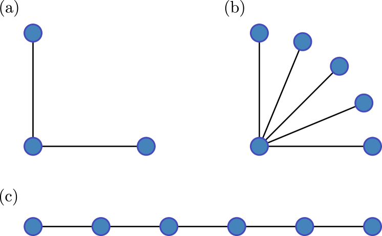
Figure 1: Three exemplary graph states: (a) For three qubits, the GHZ state and the LC state coincide. The star graph in (b) corresponds to the GHZ state of six qubits, whereas the line graph in (c) is associated to the LC state of six qubits.

Different graphs may lead to graph states that are connected by a local unitary (LU) transformation, which does not change the entanglement properties. A special class of LU transformations are local Clifford operations [29], that can be described by a graphical rule called local complementation. A local complementation in vertex $i$ transforms a graph $G=(V,E)$ into a graph $G^{\prime}=(V,E^{\prime})$ by inverting the neighbourhood $\mathcal{N}(i)$ of vertex $i$. For two vertices $j,k\in\mathcal{N}(i)$, if $(j,k)\in E$ then $(j,k)\notin E^{\prime}$ and vice versa. The set of vertices $V$ is unchanged.

In addition, graph states have also another benefit. For all graph states there is an associated Bell inequality known that is maximally violated by the graph state [10]. Specifically, for tree graphs, i.e., connected graphs that do not contain a cycle, the violation increases exponentially in the number of qubits $n$ [10], i.e., the ratio $D_{n}^{\text{}}$ increases exponentially in $n$. This facilitates the observation of a Bell violation. Suppose in an experiment the noisy graph state $\rho=\alpha\outerproduct{G}{G}+(1-\alpha)\mathbbm{1}/2^{n}$ is prepared. The expectation value of the Bell operator is $\langle{\mathcal{B}_{n}^{\text{}}}\rangle_{\rho}=\alpha Q_{n}^{\text{}}$. A violation is thus observed for

$$\alpha>\frac{C_{n}^{\text{}}}{Q_{n}^{\text{}}}=D_{n}^{-1},$$ (4)

which decreases exponentially with the number of qubits $n$.

We conclude this section by discussing two specific Bell inequalities for the graph states in Fig. 1. For the $n$-qubit GHZ state, Mermin’s inequality constitutes a known Bell inequality [5, 30]. Mermin’s inequality is up to local rotations equivalent to the Bell operator

$$\mathcal{B}_{n}^{\text{GHZ}}=g_{1}\prod_{i=2}^{n}(\mathbbm{1}+g_{i}),$$ (5)

where $g_{i}$ are the stabilizing operators defined in Eq. (1). The quantum bound $Q_{n}^{\text{GHZ}}=2^{n-1}$ is achieved for the $n$-qubit GHZ state. The classical bound and thus the maximal ratio $D^{\text{}}$ for Mermin’s inequality are

$$\begin{split}C_{n}^{\text{GHZ}}=\begin{cases}2^{\frac{n-1}{2}},\\ 2^{\frac{n}{2}},\end{cases},\leavevmode\nobreak\ D_{n}^{\text{GHZ}}=\begin{cases}2^{\frac{n-1}{2}},&n\leavevmode\nobreak\ \text{odd},\\ 2^{\frac{n-2}{2}},&n\leavevmode\nobreak\ \text{even}.\end{cases}\end{split}$$ (6)

For the LC state in turn we consider the Bell inequalities in Ref. [30] that are defined in case the number of qubits is a multiple of three. The Bell operator is

$$\mathcal{B}_{n}^{\text{LC}}=\prod_{\begin{subarray}{c}i=1\end{subarray}}^{n/3}(\mathbbm{1}+g_{3i-2})g_{3i-1}(\mathbbm{1}+g_{3i}),$$ (7)

which takes the maximal value for the $n$-qubit LC state. As all terms in Eq. (7) are stabilizing operators of the LC state, we have $Q_{n}^{\text{LC}}=4^{n/3}$. The classical bound in turn is

$$C_{n}^{\text{LC}}=2^{n/3}\qquad\text{and thus}\qquad D_{n}^{\text{LC}}=2^{n/3}.$$ (8)

III Methods

The Bell operators in Sec. II rely on a number of contexts that scales exponentially in the number of qubits $n$, i.e., there are in principle an exponential number of terms to measure. The number of observables thus quickly becomes infeasible. In this section, we introduce a general method to evaluate a Bell inequality by sampling random terms. The terms of the Bell inequality are picked according to a uniform probability distribution. This approach stands in line with previous schemes that use randomization to reduce the number of measurements, e.g., direct fidelity estimation [35, 36] or few-copy entanglement detection [37]. Finally, there exist different methods to assess the statistical strength of Bell tests [39, 40, 41, 42]. We gauge the significance of a violation with the help of the $p$-value. For this purpose, we start by formulating a Bell test as a hypothesis test.

III.1 Hypothesis test

The task is to evaluate a general Bell inequality with classical bound $C$, i.e., to check the inequality

$$\langle{\mathcal{B}^{\text{}}}\rangle\leq C.$$ (9)

The expectation value on the right hand side however cannot be inferred exactly in an experiment. Rather the expectation value has to be estimated from multiple experimental repetitions. For this purpose it is useful to consider an unbiased estimator $\langle{\hat{\mathcal{B}^{\text{}}}}\rangle$, which we denote by a hat. An estimator $\langle{\hat{\mathcal{B}^{\text{}}}}\rangle$ is a function of the experimental data and it is unbiased in case it reproduces the actual value in expectation, i.e., $\mathbb{E}[\langle{\hat{\mathcal{B}^{\text{}}}}\rangle]=\langle{\mathcal{B}^{\text{}}}\rangle$.

Due to the finite statistics, however, the estimate $\langle{\hat{\mathcal{B}^{\text{}}}}\rangle$ fluctuates. There is thus a non-zero probability to observe a violation of the Bell inequality although the actual state does not violate it. To quantify the probability that an observed violation is only due to statistical fluctuations, we formulate the Bell test as a hypothesis test. The hypotheses are

• Null hypothesis $\mathbf{H_{0}}$: The measurement outcomes can be described by a local hidden variable (LHV) model,

• Alternative hypothesis $\mathbf{H_{1}}$: The Bell inequality is violated.

To gauge whether the observed data is in contradiction with the null hypothesis $H_{0}$, we look at the $p$-value. The $p$-value is defined as the probability to observe an estimate at least as large as some value $\theta$ in case $H_{0}$ is true, i.e.,

$$p=\mathbb{P}\left(\langle{\hat{\mathcal{B}^{\text{}}}}\rangle>\theta\leavevmode\nobreak\ \big{|}\leavevmode\nobreak\ H_{0}\right).$$ (10)

But the $p$-value is hard to calculate since the probability depends on the probability distribution of the estimator $\langle{\hat{\mathcal{B}^{\text{}}}}\rangle$ which is unknown. We can, however, upper bound the $p$-value. A local theory can at most reach a value of $\langle{\mathcal{B}^{\text{}}}\rangle=\mathbb{E}[\langle{\hat{\mathcal{B}^{\text{}}}}\rangle]=C$. Thus, in case $H_{0}$ is true the estimator $\langle{\hat{\mathcal{B}^{\text{}}}}\rangle$ has to exceed its mean by at least $t=\theta-C$ if a violation $\langle{\hat{\mathcal{B}^{\text{}}}}\rangle=\theta>C$ is observed. This is sketched in Fig. 2. We consequently obtain the upper bound

$$p\leq\mathbb{P}(\langle{\hat{\mathcal{B}^{\text{}}}}\rangle-\langle{\mathcal{B}^{\text{}}}\rangle\geq t).$$ (11)

In the following we use Hoeffding’s inequality [43] to upper bound the right hand side of Eq. (11). Hoeffding’s inequality is a large deviation bound that typically involves the number of repetitions. This allows us to connect the number of repetitions to the $p$-value. Finally, we say that an observed result has a confidence level of $\gamma=1-p$.

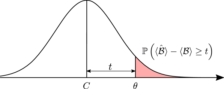
Figure 2: Upper bound of the $p$-value. To observe a value of $\theta>C$ even though the state obeys the classical bound, the estimator $\langle{\hat{\mathcal{B}}}\rangle$ has to exceed its mean by at least $t$.

III.2 Random sampling

So far, we have noted that there are multipartite Bell inequalities known that adapt to the architecture of the quantum computer and show a growing resistance to white noise. This allows to overcome problem (i) and (ii). We have seen however that also the number of terms grows exponentially, which makes it experimentally infeasible to measure all terms. In this section, we describe a scheme to overcome this problem and which allows to evaluate the Bell inequalities.

A general Bell operator $\mathcal{B}$ can be written as a sum of observables:

$$\mathcal{B}^{\text{}}=\sum_{j=1}^{M}B_{j}.$$ (12)

We note that for the Bell inequalities in Sec. II the number of terms equals the quantum bound, i.e., $M=Q_{n}$. We propose to estimate the expectation value of the Bell operator by measuring the expectation value of $L$ randomly chosen terms. To analyse how many terms $L$ have to be sampled, we first assume that the expectation values can be inferred directly, i.e., we consider the limit of infinite measurements. With this simplification, the estimator reads

$$\langle{\hat{\mathcal{B}}}\rangle_{\infty}=\frac{M}{L}\sum_{l=1}^{L}\langle{B_{J_{l}}}\rangle.$$ (13)

We note that in the above expression $J_{1},\ldots,J_{L}$ are independent random variables with possible outcomes in the range $\{1,\ldots,M\}$. We assume that all outcomes are equally likely, i.e., $\mathbb{P}(J_{l}=j)=\frac{1}{M}$ for all $j\in\{1,\ldots,M\}$. In App. A.1, we show that the estimator is unbiased, i.e., $\mathbb{E}[\langle{\hat{\mathcal{B}}}\rangle_{\infty}]=\langle{\mathcal{B}}\rangle$.

To assess the significance of an observed violation, we consider the $p$-value. We upper bound the $p$-value with the help of Eq. (11). The probability on the right hand side of Eq. (11) can be bounded with the help of concentration inequalities. Here, we consider Hoeffding’s inequality, which yields

$$p\leq\mathbb{P}(\langle{\hat{\mathcal{B}}}\rangle_{\infty}-\langle{\mathcal{B}}\rangle\geq t)\leq\exp\left(-\frac{t^{2}}{2M^{2}}L\right).$$ (14)

The details on Hoeffding’s inequality are presented in App. B.1. This result can be used to derive a lower bound on the necessary $L$. To reach a confidence level of $\gamma=1-p$,

$$L\geq\left\lceil-\frac{2M^{2}}{t^{2}}\log(1-\gamma)\right\rceil$$ (15)

random terms of the Bell operator have to be sampled.

III.3 Number of measurement repetitions

We now take into account that the expectation values cannot be inferred directly. Rather, the measurement of each chosen term $B_{j}$ has to be repeated multiple times. In this section, we are interested in how many repetitions are necessary. For this purpose, we adjust the estimator in Eq. (13) to include the measurement repetitions. We assume that every term is measured $K$-times. This yields the estimator

$$\langle{\hat{\mathcal{B}}}\rangle=\frac{M}{KL}\sum_{l=1}^{L}\sum_{k=1}^{K}b_{J_{l}}^{(k)}.$$ (16)

In the above estimator, $b_{j}^{(k)}$ denotes the measurement outcome of the term $B_{j}$ in the $k$-th repetition. Thus, we have $b_{j}^{(k)}\in\{\pm 1\}$. As in Eq. (13), $J_{1},\ldots,J_{L}$ denote independent random variables that uniformly distributed take values from $\{1,\ldots,M\}$. We show in App. A.2 that also the estimator in Eq. (16) is unbiased, i.e., $\mathbb{E}[\langle{\hat{\mathcal{B}}}\rangle]=\langle{\mathcal{B}}\rangle$. Finally, we can again use Eq. (11) and Hoeffding’s inequality to bound the $p$-value:

$$p\leq\mathbb{P}(\langle{\hat{\mathcal{B}}}\rangle-\langle{\mathcal{B}}\rangle\geq t)\leq\exp(-\frac{t^{2}}{2M^{2}}KL).$$ (17)

However, we have already derived a lower bound for $L$. We thus obtain a lower bound on $K$ from Eq. (17):

$$K\geq\frac{1}{L}\left\lceil-\frac{2M^{2}}{t^{2}}\log(1-\gamma)\right\rceil.$$ (18)

Since $L\geq\lceil-\frac{2M^{2}}{t^{2}}\log(1-\gamma)\rceil$, we observe that $K\geq 1$. As a result, we can conclude that it is sufficient to measure each term only once.

IV Analysis of the Bell inequalities for the GHZ and LC state

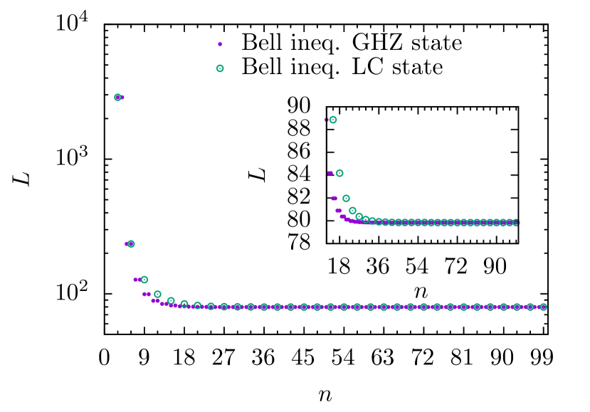
Figure 3: Necessary number of random observables $L$, which are measured $K=1$ times each, such that an observed violation of at least $\langle{\hat{\mathcal{B}^{\text{}}}}\rangle=\alpha Q_{n}$ for $\alpha=0.6$ has a confidence of $\gamma=5\sigma$.

In this section, we are going to apply the method to the Bell inequalities for graph states. Especially, we will look at the Bell inequalities for the GHZ and the LC state. As described in the motivation, these Bell inequalities are promising to detect a large violation.

For this purpose, we express the observed expectation value as a fraction $\alpha$ of the quantum bound, i.e.,

$$\langle{\hat{\mathcal{B}^{\text{}}}}\rangle=\alpha Q_{n}.$$ (19)

As we have seen in Eq. (4), to observe a violation of the Bell inequality we have to have $\alpha>D_{n}^{-1}\overset{n\rightarrow\infty}{\rightarrow}0$. In case a violation is observed, it is $t=\alpha Q_{n}-C_{n}$. The number of random terms that are necessary to ensure a confidence level $\gamma$ is given by Eq. (15) that takes the form

$$L\geq\left\lceil-\frac{2}{(\alpha-D_{n}^{-1})^{2}}\log(1-\gamma)\right\rceil.$$ (20)

We note that for the Bell inequalities in Sec. II, the number of terms equals the quantum bound, i.e., $M=Q_{n}$. As $D_{n}^{-1}$ converges to zero in the limit $n\rightarrow\infty$, we can conclude that $L$ converges against some constant value for fixed $\alpha$. This is shown for the Bell inequalities associated to the GHZ and LC state in Fig. 3.

For both the GHZ state as well as the LC state, we have assumed an observed violation of $\langle{\hat{\mathcal{B}^{\text{}}}}\rangle=\alpha Q_{n}$ with $\alpha=0.6$. This moreover implies that the assumed violation increases with the number of qubits $n$. We thus stress that Fig. 3 is only valid in case at least a value $\langle{\hat{\mathcal{B}^{\text{}}}}\rangle=\alpha Q_{n}$ is observed and does not show the generic scaling of $L$ with $n$. Exemplary we can make the observation:

Observation 1.

In case a violation $\langle{\hat{\mathcal{B}^{\text{}}}}\rangle=\alpha Q_{n}$ of the Bell inequality associated to the GHZ state or the LC state for $n=81$ qubits has been observed by sampling $L=80$ random terms, the result has a confidence level of $\gamma=5\sigma$.

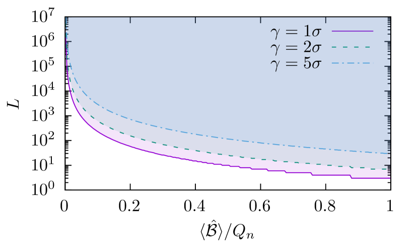
Figure 4: Confidence levels $\gamma$ for an observed violation $\langle{\hat{\mathcal{B}^{\text{}}}}\rangle$ with $L$ random terms ($K=1$) in case the classical bound $C_{n}$ is negligible compared to the observed violation $\langle{\hat{\mathcal{B}}}\rangle$.

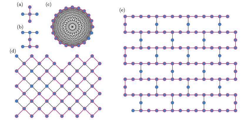
Figure 5: Connectivities of different quantum computers. The connectivity graph in (a) is used for example by the the Starmon-5 quantum processor [44], whereas IBM’s Falcon processor [45] is based on layout (b). (c) shows the connectivity of the ion trap quantum computer in Ref. [46]. Finally, in (d) we depict the connectivity graph of Google’s Sycamore processor [13] and in (e) IBM’s Eagle processor ibm_brisbane [45].

We note that for small $n$, $L$ exceeds the number of contexts of the Bell operator. This, however, is not a contradiction as we do not exclude that a term is sampled multiple times.

In addition, Eq. (20) shows that with increasing $L$ a decreasing violation $\langle{\hat{\mathcal{B}^{\text{}}}}\rangle=\alpha Q_{n}$ with $\alpha\sim\mathcal{O}(L^{-1/2})$ can be verified.

Finally, we see in Fig. 3 that already for relatively small $n$ the classical bound $C_{n}$ becomes negligible compared to the observed violation $0.6\times Q_{n}$. Therefore, it does not have an effect on $L$ for large $n$. We thus show the contours of the confidence levels $\gamma=1\sigma,2\sigma$ and $5\sigma$ in the limit $n\rightarrow\infty$ for a given observation $\langle{\hat{\mathcal{B}^{\text{}}}}\rangle$ with $L$ random terms in Fig. 4.

V Bell nonlocality as benchmark

We now discuss Bell nonlocality as a benchmark for quantum computers. We will investigate the Bell violations that can be achieved on current quantum computers. For this purpose, we first consider the connectivity graphs of different quantum computers and discuss what Bell inequalities can be used. Afterwards, we include noise to assess realistic violations.

V.1 Connectivities of current quantum computers

We start by having a look at the connectivity graphs of different quantum computers and the Bell inequalities that can be evaluated on the different architectures. In Fig. 5, we show the connectivity graphs of few current quantum computers. The first connectivity in Fig. 5a is the star graph of five qubits, i.e., one central qubit connected to four other qubits. This layout is used, e.g., in the Starmon-5 quantum processor [44]. Fig. 5b shows the connectivity graph that is used by IBM’s Falcon processor [45]. The ion trap quantum computer in Ref. [46] has 20-qubits that can all be coupled. The corresponding connectivity graph is shown in Fig. 5c. We also include the connectivity graphs of Google’s Sycamore processor in Fig. 5d [13] that has $53$ qubits and IBM’s Eagle processor [45] that has $127$ qubits.

As the optimal Bell inequality that is associated to the connectivity graph is in general hard to determine, we will focus on the Bell inequalities for the GHZ and the LC state. In the following, we are interested in the largest GHZ and LC state that can be natively prepared on the different layouts in Fig. 5, i.e., that can be prepared by the available two-qubit gates only.

Observation 2.

On a quantum computer of $n$ qubits, it is always possible to prepare a GHZ state of all $n$ qubits with a circuit of $\mathcal{O}(n)$ depth.

Proof.

The connectivity graph of quantum computers is usually connected. Thus, by the following steps a GHZ state of all $n$ qubits can be prepared. The steps are illustrated in Fig. 6 for the architecture in Fig. 5b.

1. Prepare a star graph with center at the qubit with the largest connectivity [Fig. 6b].

2. By performing two local complementations, the center of the star graph can be shifted to any node of the graph. Thus, the center can be moved to a vertex with still uncoupled neighbours [Fig. 6c-d].

3. By applying a CZ gate between the center node and the uncoupled neighbours the adjacent qubits can be added to the GHZ state [Fig. 6e].

4. Step 2+3 can be repeated until all qubits are coupled.

This procedure requires at least $n-1$ consecutive CZ gates. In the worst case, there are two local complementations needed between all CZ gates. Combined with the initial Hadamard gates, the circuit depth is $3n+1$. ∎

We point out that the GHZ state can also be prepared in logarithmic step complexity [47, 48], depending on the connectivity.

For the LC state in contrast, we make the following observation.

Observation 3.

Assume that the connectivity graph of a quantum computer is connected. Then, a linear cluster state containing all $n$ qubits can be prepared with a circuit depth of $\mathcal{O}(n)$. In practice, however, it is often beneficial to prepare the LC state that is associated to the longest simple path in the connectivity graph [36]. The corresponding circuit has a constant depth of three independent of the number of qubits.

Proof.

We show in App. C that it is always possible to prepare a LC state that contains all qubits in linear circuit depth. The longest simple path, in contrast, can be generated by first preparing all qubits in the $\ket{+}$ state, i.e., by applying Hadamard gates. Afterwards, every second CZ gate can be performed in parallel. The circuit depth is thus three independent of the length of the simple path. The circuit is shown for the $6$-qubit LC state in Fig. 7a. ∎

As we only know the Bell inequality for the LC state with a number of qubits that is a multiple of three, we search for the longest path of length divisible by three. The longest paths that fulfill this restriction are drawn pink in Fig. 5. The connectivity graphs in Fig. 5a and Fig. 5b allow to prepare a $3$-qubit LC state. The largest simple path on the $20$-qubit full-connectivity graph in Fig. 5c with length divisible by three has length $18$. The quantum computer in Fig. 5c thus allows to check the Bell inequality for the $18$-qubit LC state. To find the longest path is an NP-complete problem [49]. We can thus not verify if the marked paths for the layouts in Fig. 5d and Fig. 5e are indeed the longest paths. In Fig. 5d, we have identified a $48$-qubit path as longest simple path. The layout in Fig. 5e in turn allows the preparation of the $108$-qubit LC state.

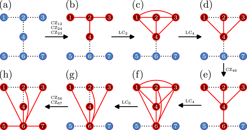
Figure 6: Preparation scheme for the GHZ state on the $7$-qubit interaction topology that is for example used by IBM’s Falcon processor. The dotted lines indicate the physical CZ gates, whereas the graph state is drawn in red.

V.2 Noise

In the following section, we will discuss the effect of noise. The goal is to roughly estimate the violation that can be realistically observed on quantum computers. Commonly, the errors of quantum computers are specified in terms of the error rates for single-qubit gates, two-qubit gates and readout. The error rates for IBM’s Eagle processor ibm_brisbane and Google’s Sycamore processor are shown in Tab. 1. The error rate for the single-qubit gates is typically about an order smaller than the other error rates. We thus neglect the single-qubit errors. The readout error on the other side can be mitigated by classical post-processing [50, 51]. We thus focus on the error in the two-qubit gates. For this purpose, we will consider a simple depolarisation noise model.

	Single-qubit gate	Two-qubit gate	Readout
IBM Eagle	$2.417\times 10^{-4}$	$7.409\times 10^{-3}$	$1.390\times 10^{-2}$
Google Sycamore
isolated	$1.5\times 10^{-3}$	$3.6\times 10^{-3}$	$3.1\times 10^{-2}$
simultaneous	$1.6\times 10^{-3}$	$6.2\times 10^{-3}$	$3.8\times 10^{-2}$

Table 1: Error rates of IBM’s Eagle processor ibm_brisbane calibrated on 27.02.2024 18:32:14 [45] and Google’s Sycamore processor [13]. Google gives the error rates for the cases that the gates are performed isolated or simultaneously on all qubits.

In the depolarisation noise model, we assume that an error results on average in a maximally mixed state, i.e., the circuit for the graph state $\ket{G}$ prepares the mixture

$$\rho=p\outerproduct{G}{G}+(1-p)\frac{\mathbbm{1}}{2^{n}}.$$ (21)

The probability that no error in the two-qubit gates occurs is $p=(1-p_{2})^{N_{2}}$, where $p_{2}$ is the error rate and $N_{2}$ the number of the two-qubit gates. The observed violation is thus

$$\expectationvalue{\mathcal{B}}=p\times Q_{n}.$$ (22)

Figure 7: Quantum circuits to prepare (a) the LC state and (b) the GHZ state for $n=6$ qubits. The circuits make use of the Hadamard gate denoted by $H$ and CZ operations that are represented by the connected dots.

In Fig. 7, we show the circuits to prepare the LC and GHZ state in the case of $n=6$ qubits. For the LC state the CZ gates can be performed simultaneously and thus the circuit exhibits a constant depth of three independent of the number of qubits. For the GHZ state however the preparation with CZ gates requires the gates to be applied consecutively. The circuit depth thus grows with the number of qubits. The number of CZ gates, however, is equal.

	Violation $\langle{\mathcal{B}}\rangle/Q$	$L$ for $\gamma=5\sigma$
Google Sycamore
LC state ($n=48$)	$0.6913$	$41$
GHZ state ($n=53$)	$0.7656$	$34$
IBM ibm_brisbane
LC state ($n=108$)	$0.4396$	$102$
GHZ state ($n=127$)	$0.3800$	$136$

Table 2: Results for the depolarisation noise model that takes the 2-qubit gate error into account. For the noise data of Google’s Sycamore [13] and IBM’s Eagle processor [45] we show the violations in terms of the quantum bound $Q$. The last column shows the number of random terms $L$ that have to be sampled to verify the violation with a confidence of $5\sigma$.

The results in Tab. 2 show that the simple noise model predicts a violation of more than $0.6\times Q$ for Google’s Sycamore processor and a bit less for ibm_brisbane. We note however that we considered more qubits on the IBM machine. A violation can thus be verified on both machines with $L\sim\mathcal{O}(10)-\mathcal{O}(10^{2})$. This is of the same order as in Sec. IV. However, we stress that the considered noise model does not take the 1-qubit gate errors and readout errors into account. Real quantum computers moreover do not implement all gates natively. IBM’s Eagle processor for example does not support the CZ gate. Rather, it has to be composed by the available gates. The circuit in practice thus contains more gates and possibly exhibits a larger depth. For these reasons the noise model probably overestimates the violation. However, it is still interesting to note that the noise model predicts the number of samples $L$ to increase exponentially in $n$. This is shown in Fig. 8.

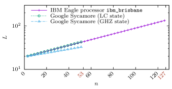
Figure 8: Number of terms $L$ that have to be sampled to verify the violation predicted by the depolarisation noise model with a confidence level of $\gamma=5\sigma$.

VI Simulation for an IBM quantum computer

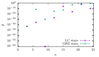
Figure 9: Average p-value of the results for the LC and GHZ state in Fig. 10. The average is taken over the p-values of the $10$ repetitions. The error bars denote the standard deviation. We plot only the top error bars as we are interested in the uncertainty to larger $p$-values.

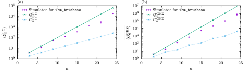
Figure 10: Simulation for the IBM Eagle quantum processor. The simulation uses the error rates of the real device ibm_brisbane [45] and the violation is estimated by measuring $L=800$ random terms of the Bell inequality $K=1$ times each. In (a) the average expectation value of the Bell inequality $\mathcal{B}^{\text{LC}}$ is shown for the LC state, whereas (b) shows the violation of $\mathcal{B}^{\text{GHZ}}$ for the GHZ state. In both cases, the expectation values are averaged over $10$ repetitions and the error bars show the standard deviation.

Finally, we simulate the Bell inequalities of the LC and the GHZ state for the IBM Eagle quantum processor. For this purpose, we use the Qiskit AerSimulator [52] with the noise data of the quantum computer ibm_brisbane available at [45]. In Fig. 7, we show the ideal circuits to prepare the LC and the GHZ state for $n=6$ qubits. The advantage of the LC state is that it can be prepared by a circuit of constant depth of three, whereas the step complexity for the GHZ state increases with the number of qubits $n$. We note, however, that IBM’s Eagle processor does not implement the Hadamard and CZ gate natively. Rather, the gates have to be composed in terms of the available gate set. In practice the circuits thus involve more gates and exhibit a larger depth.

After the preparation, $L$ random terms of the corresponding Bell inequality are measured. The measurement of each random term is not repeated, i.e., $K=1$. Fig. 10 shows the average expectation values of the Bell inequalities for the LC and GHZ state of up to $n=24$ qubits. We have chosen $L=800$ random terms and the average is taken over $10$ repetitions. Moreover, the number of qubits is a multiple of three as only in this case a good Bell inequality for the LC state is known. Fig. 10 shows that for both states the simulation predicts a Bell violation that increases exponentially with $n$. The LC state however shows a slightly higher relative violation compared to the GHZ state. This can be seen in Fig. 11a. The plot in Fig. 11a displays the observed violation as a fraction of the total number of terms in the Bell inequality, i.e., $t^{2}/M^{2}=(\langle{\hat{\mathcal{B}}}\rangle-C_{n})^{2}/M^{2}$. We fit the data points to an exponential and obtain

$$\begin{split}\left(\frac{t^{2}}{M^{2}}\right)_{\text{LC}}(n)=\exp(-0.10n-0.65),\\ \left(\frac{t^{2}}{M^{2}}\right)_{\text{GHZ}}(n)=\exp(-0.17n-0.54).\end{split}$$ (23)

This affirms that the relative violation of the GHZ state decreases faster with $n$ compared to the LC state. We attribute this to the larger circuit depth that is required for the GHZ state. The preparation of the GHZ state is thus more affected by noise. The smaller relative violation is also the reason for the larger $p$-values for the GHZ state, which we present in Fig. 9. Except for the cases of $n=3,15$ the $p$-values of the LC state are smaller, which implies a higher significance of the observed violation.

Finally, we use Eq. (23) to extrapolate the violation to larger $n$. Hoeffding’s inequality in Eq. (17) yields for $K=1$ and a target value for the confidence $\gamma$:

$$L(n,\gamma)\geq\left\lceil-\frac{2}{(t^{2}/M^{2})(n)}\log(1-\gamma)\right\rceil.$$ (24)

The number of necessary sampled terms $L$ is shown in Fig. 11b for the LC state and in Fig. 11c for the GHZ state. We first point out the different scaling of $L$ compared to Fig. 3. Whereas in Fig. 3 $L$ decreases with $n$ until a plateau is reached, Fig. 11 suggests that $L$ increases exponentially with $n$. This however can be attributed to fact that Fig. 3 has been obtained with the assumption that the relative violation stays constant with the number of qubits $n$. But Fig. 11a indicates that this assumption is not true for a real quantum computer. However, we still obtain that the number of terms $L$ that have to be sampled is much smaller than the total number of terms $M$.

As an example, we discuss $L$ for the case of $n=81$ qubits and a target confidence of $\gamma=5\sigma$:

$$\begin{split}L_{\text{LC}}(n=81,\gamma=5\sigma)&=182813,\\ L_{\text{GHZ}}(n=81,\gamma=5\sigma)&=47170845.\end{split}$$ (25)

The above numbers are much smaller than $M_{\text{LC}}\approx 10^{16}$ and $M_{\text{GHZ}}\approx 10^{24}$, but larger than the values predicted in Sec. IV. As previous, we attribute this to the unrealistic assumption that independent of $n$ a violation $\langle{\mathcal{B}_{n}}\rangle=0.6\times Q_{n}$ can be observed. For $n=24$ qubits the simulation yields $\langle{\hat{\mathcal{B}}^{\text{LC}}_{n}}\rangle/Q^{\text{LC}}_{n}=0.28$ for the LC state and $\langle{\hat{\mathcal{B}}^{\text{GHZ}}_{n}}\rangle/Q^{\text{GHZ}}_{n}=0.09$ for the GHZ state, which is already much smaller than $0.6$ in both cases.

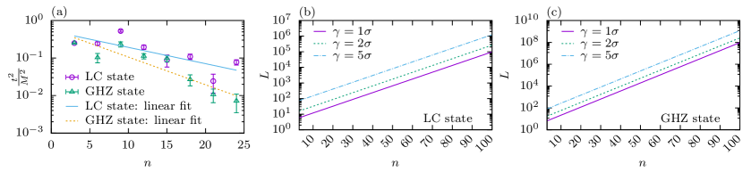
Figure 11: (a) Observed violation in relation to the number of terms in the Bell inequality, i.e., $t^{2}/M^{2}=(\langle{\hat{\mathcal{B}}}\rangle-C_{n})^{2}/M^{2}$. The data points are fitted by an exponential. From the fitted function $t^{2}/M^{2}$ we estimate the number of random terms $L$ that have to be sampled to reach a confidence of $\gamma=1\sigma,2\sigma,5\sigma$. (b) shows the results for the LC state, whereas (c) illustrates the predictions for the GHZ state.

VII Conclusion

We have demonstrated a method to test $n$-partite Bell nonlocality on quantum computers. Quantum computer often have restricted two-qubit connectivity. We have thus pointed out that graph states are a natural choice of nonlocal states that can be readily prepared if the graph is a subgraph of the connectivity graph. Moreover, for certain graph states good Bell inequalities are known. These Bell inequalities allow for an exponential violation of the classical bound, but in turn also typically require an exponential number of measurements. On the one hand, the exponential violation makes them increasingly robust to noise. On the other hand, it is impossible to measure all terms in an experiment. We have solved this problem by proposing a method in the manner of randomized measurements, e.g., direct fidelity estimation [35, 36] or few-copy entanglement detection [37]. By sampling the terms of the Bell operator at random the number of measurements can be drastically reduced. The violation can, however, still be verified with high significance. We have gauged the significance of a result with Hoeffding’s inequality. It thus dependents on the violation observed. To assess the usefulness of the method on real devices, we have first used a simple depolarisation noise model to estimate realistic violations. Finally, we have simulated the method for the IBM Eagle quantum processor. As expected with increasing accuracy of the noise model the predicted violation shrinks. However, also the simulator of the IBM processor predicts the number of terms that have to be sampled to be much smaller than the total number of terms in the Bell inequalities.

Our method will hence be useful to verify Bell violations in quantum systems of many qubits. This includes current quantum computers in the NISQ regime, e.g., the quantum computers accessible at IBM Quantum [45]. In addition, the observed Bell violation can be used to benchmark and compare different quantum computers. The Bell violation can be interpreted as a measure for the nonclassical correlations that can be produced. The preparation of the associated state depends on the connectivity of the quantum computer. We thus can benchmark the nonclassical correlations for states that require different levels of two-qubit connectivity. Finally, we stress that our method is not restricted to qubits and can be readily applied to Bell inequalities with higher local dimension.

Furthermore, the method could also be refined. For example, as the Bell inequalities only include stabilizers of the graph state, all observables commute. It might thus be feasible to find a (possibly very complicated) POVM to simultaneously measure all terms.

Moreover, it could be interesting to analysis the Bell inequalities with other statistical methods. Instead of the $p$-value, one might look at the Kullback–Leibler divergence that has been used to assess the statistical strength of Bell inequalities for few parties [40].

The relation to other benchmarks, e.g., the quantum volume [53, 54] or the layer fidelity [55], is also yet to be explored. Especially the layer fidelity can be measured by benchmarking a linear string of qubits of the quantum computer.

Appendix A Unbiased estimators

In this appendix, we show that the estimators used in the main text are unbiased.

A.1 Estimator in the infinite measurement limit

First, we assume that the expectation values can be inferred directly, i.e., that we can repeat the measurement of the operator infinite times. In this case, the estimator is given by Eq. (13). The expectation value has to be calculated with respect to the random variables $J_{l}$. With $\mathbb{E}[\langle{B_{J_{l}}}\rangle]=\sum_{j=1}^{M}p(J_{l}=j)\langle{B_{j}}\rangle=\frac{1}{M}\sum_{j=1}^{M}\langle{B_{j}}\rangle$ we obtain

$$\begin{split}\mathbb{E}[\langle{\hat{\mathcal{B}}}\rangle_{\infty}]=&\frac{M}{L}\sum_{l=1}^{L}\mathbb{E}[\langle{B_{J_{l}}}\rangle]=\frac{M}{L}\sum_{l=1}^{L}\frac{1}{M}\sum_{j=1}^{M}\langle{B_{j}}\rangle\\ =&\sum_{j=1}^{M}\langle{B_{j}}\rangle=\langle{\mathcal{B}}\rangle.\end{split}$$ (26)

A.2 Estimator for finite repetitions

To calculate the expectation value of the estimator in Eq. (16), we note that both the measurement outcomes $b_{j}$ and the index $J$ of the terms are random variables. Hence, the expectation value of the estimator has to be taken over both the measurement outcomes as well as the random picking, i.e., over $J$. To evaluate the expectation value we can thus make use of the law of iterated expectation. That, is,

$$\mathbb{E}[\ldots]=\mathbb{E}_{J}\left\{\mathbb{E}_{b_{J_{l}}}[\ldots|J_{l}=J]\right\}.$$ (27)

This results in

$$\begin{split}\mathbb{E}[\langle{\hat{\mathcal{B}}}\rangle]&=\frac{M}{KL}\sum_{l=1}^{L}\sum_{k=1}^{K}\mathbb{E}_{J}\Big{\{}\underbrace{\mathbb{E}_{b_{J_{l}}}[b_{J_{l}}^{(k)}|J_{l}=J]}_{=\expectationvalue{B_{J}}}\Big{\}}\\ &=\frac{M}{KL}\sum_{l=1}^{L}\sum_{k=1}^{K}\mathbb{E}_{J}[\expectationvalue{B_{J}}]\\ &=\frac{M}{KL}\sum_{l=1}^{L}\sum_{k=1}^{K}\underbrace{\sum_{j=1}^{M}p(j)\expectationvalue{B_{j}}}_{=\sum_{j=1}^{M}\frac{1}{M}\expectationvalue{B_{j}}}\\ &=\sum_{j=1}^{M}\expectationvalue{B_{j}}=\expectationvalue{\mathcal{B}}.\end{split}$$ (28)

Appendix B Hoeffding’s inequality

B.1 Estimator in the infinite measurement limit

The estimator in Eq. (13) can be written as a sum of random variables as follows:

$$\langle{\hat{\mathcal{B}}}\rangle_{\infty}=\sum_{l=1}^{L}\underbrace{\frac{M}{L}\langle{B_{J_{l}}}\rangle}_{\eqqcolon X_{l}}.$$ (29)

Since each term $B_{j}$ in the Bell operator is a tensor product of Pauli operators, $\langle{B_{j}}\rangle\in[-1,1]$ and thus $-\frac{M}{L}=a_{l}\leq X_{l}\leq b_{l}=\frac{M}{L}$. Moreover, the bounded random variables $X_{l}$ are independent, as they are obtained from different experimental runs. We can thus use Hoeffding’s inequality [43], which states that

$$\begin{split}\mathbb{P}(\langle{\hat{\mathcal{B}}}\rangle_{\infty}-\langle{\mathcal{B}}\rangle\geq t)&\leq\exp(-\frac{2t^{2}}{\sum_{l=1}^{L}(b_{l}-a_{l})^{2}})\\ &=\exp(-\frac{2t^{2}}{\sum_{l=1}^{L}(\frac{2M}{L})^{2}})\\ &=\exp(-\frac{t^{2}}{2M^{2}}L).\end{split}$$ (30)

B.2 Estimator for finite repetitions

As in the previous section, we can apply Hoeffding’s inequality to the estimator in Eq. (16). Also the estimator in Eq. (16) is a sum of independent random variables:

$$\langle{\hat{\mathcal{B}}}\rangle=\sum_{l=1}^{L}\sum_{k=1}^{K}\underbrace{\frac{M}{KL}b_{J_{l}}^{(k)}}_{\eqqcolon Y_{kl}}.$$ (31)

Since the outcomes $b_{J_{l}}^{(k)}$ are obtained from different experimental runs, they are independent and thus are the random variables $Y_{kl}$. In addition, the outcomes can only take the values $b_{J_{l}}^{(k)}\in\{-1,1\}$. Therefore, we have that the random variables $Y_{kl}$ are bounded as: $-\frac{M}{KL}=a_{kl}\leq Y_{kl}\leq b_{kl}=\frac{M}{KL}$. Finally, we get from Hoeffding’s inequality

$$\begin{split}\mathbb{P}(\langle{\hat{\mathcal{B}}}\rangle-\langle{\mathcal{B}}\rangle\geq t)&\leq\exp(-\frac{2t^{2}}{\sum_{l=1}^{L}\sum_{k=1}^{K}(b_{kl}-a_{kl})^{2}})\\ &=\exp(-\frac{2t^{2}}{\sum_{l=1}^{L}\sum_{k=1}^{K}(\frac{2M}{KL})^{2}})\\ &=\exp(-\frac{t^{2}}{2M^{2}}KL).\end{split}$$ (32)

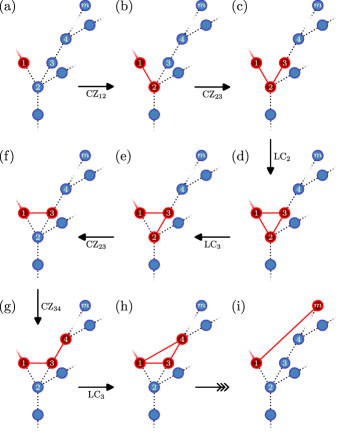
Figure 12: Scheme to decompose the CZ gate between arbitrary qubits $1$ and $m$ into a sequence of CZ gates between adjacent qubits and local complementations. The dotted lines denote the CZ gates that can be performed, whereas the red lines indicate the graph state. Qubit $1$ can already be coupled to different qubits, whereas the qubits $2,\ldots m$ have to be uncoupled.

Appendix C Preparation scheme for the LC state

We discuss a scheme to prepare a LC state with all qubits of a $n$-qubit quantum computer. This can be done by preparing all qubits in the $\ket{+}$ state and then applying CZ gates between some of them. A problem can be that the connectivity of the quantum computer does not allow to perform a specific gate between qubits $i$ and $j$ directly. The following lemma shows that this is not a fundamental problem.

Lemma 1.

Consider a qubit array with a connected connectivity graph, where a CZ gate should be applied to two qubits for graph state generation from the state $\ket{+}^{\otimes n}$. This can be achieved by a sequence of CZ gates between adjacent qubits (in the sense of the connectivity graph) and local complementations.

Proof.

We give an explicit construction that is visualized in Fig. 12. The initial state is shown in Fig. 12a. We would like to perform a CZ gate between qubits $1$ and $m$, i.e., $\text{CZ}_{1m}$. The interaction topology, however, does not allow a direct coupling. Rather the qubits $1$ and $m$ are connected by the path of qubits $1,2,\ldots m$. Here, all the qubits $1,2,\ldots m$ should be in the $\ket{+}$ state, especially, it is important that no CZ gate has been applied to the qubits $2,\ldots m$ yet. In this case, we can apply the following scheme:

1. Connect qubit $2$ by performing the $\text{CZ}_{12}$ gate to generate the first $\text{PAIR}(1,2)$ (Fig. 12b).

2. While $k<m$ transform $\text{PAIR}(1,k)\rightarrow\text{PAIR}(1,k+1)$ by

   1. Couple qubit $k$ and $k+1$ by $\text{CZ}_{k,k+1}$ (Fig. 12c).

   2. Couple qubit $1$ and $k+1$ by a local complementation on qubit $k$, i.e., $\text{LC}_{k}$ (Fig. 12d).

   3. Cancel the CZ gate between qubits $1$ and $k$ by performing $\text{LC}_{k+1}$ (Fig. 12e).

   4. Cancel the CZ gate between qubits $k$ and $k+1$ by the controlled-Z $\text{CZ}_{k,k+1}$ (Fig. 12f).

This allows to decompose the $\text{CZ}_{1m}$ gate into a sequence with circuit depth $3(m-2)+1$. We note that step $2$ is only necessary for $m>1$ and requires three steps as the local complementations in (b) and (c) can be combined. ∎

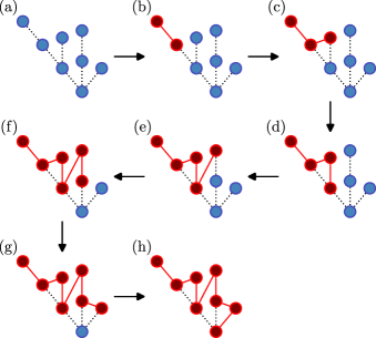
Figure 13: Illustration of the scheme in Obs. 4 for an exemplary two-qubit connectivity of eight qubits. The dotted lines denote the CZ gates that can be performed, whereas the red lines indicate the graph state.

Lemma 1 can be used to construct a linear cluster state on an arbitrary interaction topology.

Observation 4.

On a quantum computer of $n$-qubits it is possible to prepare a $n$-qubit LC state with $\mathcal{O}(n)$ circuit depth.

Proof.

The connectivity of a quantum computer is a connected graph $G$. It thus has a spanning tree, i.e., a tree graph that covers all vertices of $G$. A tree graph in turn can be covered by a LC state by the following steps. At the start, all qubits are assumed to be prepared in the state $\ket{+}^{\otimes n}$.

1. We start at a leaf and successively couple the adjacent qubits in direction of the root by CZ operations.

2. At a branch-off, check whether the other branch has already been covered. If all other branches have already been covered, we continue step $1$ in direction of the root. Otherwise, Lemma 1 can be used to couple the last qubit to a leaf in the uncovered branch. From there we can continue again with step $1$.

The scheme is shown for an exemplary two-qubit connectivity in Fig. 13. To investigate the circuit depth, we note that step $1$ and $2$ are executed alternately. We thus count the number of steps for each run. $k_{i}$ denotes the number of steps for the $i$-th execution of step $1$, whereas $l_{i}$ stands for the steps required for the $i$-th execution of step $2$. In step $1$, adjacent qubits are coupled consecutively by CZ gates. We thus have $\sum_{i}k_{i}<n$. In each step $2$, a qubit at distance $m_{i}$ is coupled and from Lemma 1 we know that $l_{i}=3(m_{i}-2)+1$. As each branch is only passed once, we have $\sum_{i}(m_{i}-2)\leq n$. Moreover, there are less than $n$ branch-offs, i.e., $\sum_{i}1\leq n$. Therefore, we obtain $\sum_{i}l_{i}=\sum_{i}3(m_{i}-2)+1\leq 4n$. The final circuit depth of the scheme is thus upper bounded by $\sum_{i}(k_{i}+l_{i})\leq n+4n=5n$. ∎

References

- Brunner et al. [2014] N. Brunner, D. Cavalcanti, S. Pironio, V. Scarani, and S. Wehner, Bell nonlocality, Rev. Mod. Phys. 86, 419 (2014).
- Bancal et al. [2013] J.-D. Bancal, J. Barrett, N. Gisin, and S. Pironio, Definitions of multipartite nonlocality, Phys. Rev. A 88, 014102 (2013).
- Bell [1964] J. S. Bell, On the Einstein Podolsky Rosen paradox, Phys. Phys. Fiz. 1, 195 (1964).
- Vieira et al. [2024] C. Vieira, R. Ramanathan, and A. Cabello, Test of the physical significance of Bell nonlocality (2024), arXiv:2402.00801 .
- Mermin [1990] N. D. Mermin, Extreme quantum entanglement in a superposition of macroscopically distinct states, Phys. Rev. Lett. 65, 1838 (1990).
- Chen et al. [2022] M. C. Chen, C. Wang, F. M. Liu, J. W. Wang, C. Ying, Z. X. Shang, Y. Wu, M. Gong, H. Deng, F. T. Liang, Q. Zhang, C. Z. Peng, X. Zhu, A. Cabello, C. Y. Lu, and J. W. Pan, Ruling Out Real-Valued Standard Formalism of Quantum Theory, Phys. Rev. Lett. 128, 40403 (2022).
- Jafferis et al. [2022] D. Jafferis, A. Zlokapa, J. D. Lykken, D. K. Kolchmeyer, S. I. Davis, N. Lauk, H. Neven, and M. Spiropulu, Traversable wormhole dynamics on a quantum processor, Nature (London) 612, 51 (2022).
- Cabello et al. [2008] A. Cabello, O. Gühne, and D. Rodríguez, Mermin inequalities for perfect correlations, Phys. Rev. A 77, 062106 (2008).
- Werner and Wolf [2001] R. F. Werner and M. M. Wolf, All-multipartite Bell-correlation inequalities for two dichotomic observables per site, Phys. Rev. A 64, 032112 (2001).
- Gühne et al. [2005] O. Gühne, G. Tóth, P. Hyllus, and H. J. Briegel, Bell Inequalities for Graph States, Phys. Rev. Lett. 95, 120405 (2005).
- Eisert et al. [2020] J. Eisert, D. Hangleiter, N. Walk, I. Roth, D. Markham, R. Parekh, U. Chabaud, and E. Kashefi, Quantum certification and benchmarking, Nat. Rev. Phys. 2, 382 (2020).
- Frank et al. [2024] J. Frank, E. Kashefi, D. Leichtle, and M. de Oliveira, Heuristic-free Verification-inspired Quantum Benchmarking (2024), arXiv:2404.10739 .
- Arute et al. [2019] F. Arute, K. Arya, R. Babbush, D. Bacon, J. C. Bardin, R. Barends, R. Biswas, S. Boixo, F. G. S. L. Brandao, D. A. Buell, B. Burkett, Y. Chen, Z. Chen, B. Chiaro, R. Collins, W. Courtney, A. Dunsworth, E. Farhi, B. Foxen, A. Fowler, C. Gidney, M. Giustina, R. Graff, K. Guerin, S. Habegger, M. P. Harrigan, M. J. Hartmann, A. Ho, M. Hoffmann, T. Huang, T. S. Humble, S. V. Isakov, E. Jeffrey, Z. Jiang, D. Kafri, K. Kechedzhi, J. Kelly, P. V. Klimov, S. Knysh, A. Korotkov, F. Kostritsa, D. Landhuis, M. Lindmark, E. Lucero, D. Lyakh, S. Mandrà, J. R. McClean, M. McEwen, A. Megrant, X. Mi, K. Michielsen, M. Mohseni, J. Mutus, O. Naaman, M. Neeley, C. Neill, M. Y. Niu, E. Ostby, A. Petukhov, J. C. Platt, C. Quintana, E. G. Rieffel, P. Roushan, N. C. Rubin, D. Sank, K. J. Satzinger, V. Smelyanskiy, K. J. Sung, M. D. Trevithick, A. Vainsencher, B. Villalonga, T. White, Z. J. Yao, P. Yeh, A. Zalcman, H. Neven, and J. M. Martinis, Quantum supremacy using a programmable superconducting processor, Nature (London) 574, 505 (2019).
- Šupić and Bowles [2020] I. Šupić and J. Bowles, Self-testing of quantum systems: a review, Quantum 4, 337 (2020).
- Popescu and Rohrlich [1992] S. Popescu and D. Rohrlich, Generic quantum nonlocality, Phys. Lett. A 166, 293 (1992).
- Lanyon et al. [2014] B. P. Lanyon, M. Zwerger, P. Jurcevic, C. Hempel, W. Dür, H. J. Briegel, R. Blatt, and C. F. Roos, Experimental Violation of Multipartite Bell Inequalities with Trapped Ions, Phys. Rev. Lett. 112, 1 (2014).
- Zhang et al. [2015] C. Zhang, Y.-F. Huang, Z. Wang, B.-H. Liu, C.-F. Li, and G.-C. Guo, Experimental Greenberger-Horne-Zeilinger-Type Six-Photon Quantum Nonlocality, Phys. Rev. Lett. 115, 260402 (2015).
- Pelisson et al. [2016] S. Pelisson, L. Pezzè, and A. Smerzi, Nonlocality with ultracold atoms in a lattice, Phys. Rev. A 93, 022115 (2016).
- Alsina and Latorre [2016] D. Alsina and J. I. Latorre, Experimental test of Mermin inequalities on a five-qubit quantum computer, Phys. Rev. A 94, 012314 (2016).
- Swain et al. [2019] M. Swain, A. Rai, B. K. Behera, and P. K. Panigrahi, Experimental demonstration of the violations of Mermin’s and Svetlichny’s inequalities for W and GHZ states, Quantum Inf. Process. 18, 218 (2019).
- González et al. [2020] D. González, D. F. de la Pradilla, and G. González, Revisiting the Experimental Test of Mermin’s Inequalities at IBMQ, Int. J. Theor. Phys. 59, 3756 (2020).
- Bäumer et al. [2021] E. Bäumer, N. Gisin, and A. Tavakoli, Demonstrating the power of quantum computers, certification of highly entangled measurements and scalable quantum nonlocality, npj Quantum Inf. 7, 1 (2021).
- Amouzou et al. [2022] G. Amouzou, J. Boffelli, H. Jaffali, K. Atchonouglo, and F. Holweck, Entanglement and nonlocality of four-qubit connected hypergraph states, Int. J. Quantum Inf. 20, 1 (2022).
- Yang et al. [2022] B. Yang, R. Raymond, H. Imai, H. Chang, and H. Hiraishi, Testing Scalable Bell Inequalities for Quantum Graph States on IBM Quantum Devices, IEEE J. Emerg. Sel. Top. Circuits Syst. 12, 638 (2022).
- de Boutray et al. [2021] H. de Boutray, H. Jaffali, F. Holweck, A. Giorgetti, and P. A. Masson, Mermin polynomials for non-locality and entanglement detection in Grover’s algorithm and Quantum Fourier Transform, Quantum Inf. Process. 20, 91 (2021).
- Singh et al. [2022] D. Singh, V. Gulati, Arvind, and K. Dorai, Experimental construction of a symmetric three-qubit entangled state and its utility in testing the violation of a Bell inequality on an NMR quantum simulator, EPL 140, 68001 (2022).
- Engelsen et al. [2017] N. J. Engelsen, R. Krishnakumar, O. Hosten, and M. A. Kasevich, Bell Correlations in Spin-Squeezed States of 500 000 Atoms, Phys. Rev. Lett. 118, 140401 (2017).
- Greenberger et al. [1989] D. M. Greenberger, M. A. Horne, and A. Zeilinger, Going Beyond Bell’s Theorem, in Bell’s Theorem, Quantum Theory and Conceptions of the Universe, 3 (Springer Netherlands, Dordrecht, 1989) pp. 69–72.
- Hein et al. [2006] M. Hein, W. Dür, J. Eisert, R. Raussendorf, M. Van Den Nest, and H. J. Briegel, Entanglement in graph states and its applications, Proc. Int. Sch. Phys. ”Enrico Fermi” 162, 115 (2006).
- Gühne and Cabello [2008] O. Gühne and A. Cabello, Generalized Ardehali-Bell inequalities for graph states, Phys. Rev. A 77, 032108 (2008).
- Scarani et al. [2005] V. Scarani, A. Acín, E. Schenck, and M. Aspelmeyer, Nonlocality of cluster states of qubits, Phys. Rev. A 71, 042325 (2005).
- Tóth et al. [2006] G. Tóth, O. Gühne, and H. J. Briegel, Two-setting Bell inequalities for graph states, Phys. Rev. A 73, 022303 (2006).
- Dür and Briegel [2004] W. Dür and H.-J. Briegel, Stability of Macroscopic Entanglement under Decoherence, Phys. Rev. Lett. 92, 180403 (2004).
- Ardehali [1992] M. Ardehali, Bell inequalities with a magnitude of violation that grows exponentially with the number of particles, Phys. Rev. A 46, 5375 (1992).
- Flammia and Liu [2011] S. T. Flammia and Y.-K. Liu, Direct Fidelity Estimation from Few Pauli Measurements, Phys. Rev. Lett. 106, 230501 (2011).
- Cao et al. [2023] S. Cao, B. Wu, F. Chen, M. Gong, Y. Wu, Y. Ye, C. Zha, H. Qian, C. Ying, S. Guo, Q. Zhu, H.-L. Huang, Y. Zhao, S. Li, S. Wang, J. Yu, D. Fan, D. Wu, H. Su, H. Deng, H. Rong, Y. Li, K. Zhang, T.-H. Chung, F. Liang, J. Lin, Y. Xu, L. Sun, C. Guo, N. Li, Y.-H. Huo, C.-Z. Peng, C.-Y. Lu, X. Yuan, X. Zhu, and J.-W. Pan, Generation of genuine entanglement up to 51 superconducting qubits, Nature (London) 619, 738 (2023).
- Saggio et al. [2019] V. Saggio, A. Dimić, C. Greganti, L. A. Rozema, P. Walther, and B. Dakić, Experimental few-copy multipartite entanglement detection, Nat. Phys. 15, 935 (2019).
- Gühne and Tóth [2009] O. Gühne and G. Tóth, Entanglement detection, Phys. Rep. 474, 1 (2009).
- Peres [2000] A. Peres, Bayesian Analysis of Bell Inequalities, Fortschr. Phys. 48, 531 (2000).
- VanDam et al. [2005] W. VanDam, R. Gill, and P. Grunwald, The statistical strength of nonlocality proofs, IEEE Trans. Inf. Theory 51, 2812 (2005).
- Zhang et al. [2010] Y. Zhang, E. Knill, and S. Glancy, Statistical strength of experiments to reject local realism with photon pairs and inefficient detectors, Phys. Rev. A 81, 032117 (2010).
- Elkouss and Wehner [2016] D. Elkouss and S. Wehner, (Nearly) optimal P values for all Bell inequalities, npj Quantum Inf. 2, 16026 (2016).
- Hoeffding [1963] W. Hoeffding, Probability Inequalities for Sums of Bounded Random Variables, J. Am. Stat. Assoc. 58, 13 (1963).
- QuTech [2020] QuTech, Quantum Inspire Starmon-5 Fact Sheet (2020), [Accessed: 17.11.2023].
- IBM Quantum [2021] IBM Quantum, https://quantum.ibm.com/ (2021), [Accessed: 17.11.2023].
- Friis et al. [2018] N. Friis, O. Marty, C. Maier, C. Hempel, M. Holzäpfel, P. Jurcevic, M. B. Plenio, M. Huber, C. Roos, R. Blatt, and B. Lanyon, Observation of Entangled States of a Fully Controlled 20-Qubit System, Phys. Rev. X 8, 021012 (2018).
- Cruz et al. [2019] D. Cruz, R. Fournier, F. Gremion, A. Jeannerot, K. Komagata, T. Tosic, J. Thiesbrummel, C. L. Chan, N. Macris, M.-A. Dupertuis, and C. Javerzac-Galy, Efficient Quantum Algorithms for GHZ and W States, and Implementation on the IBM Quantum Computer, Advanced Quantum Technologies 2, 1900015 (2019).
- Yu and Wei [2023] N. Yu and T.-C. Wei, Learning marginals suffices! (2023), arXiv:2303.08938 .
- Schrijver [2002] A. Schrijver, Combinatorial Optimization: Polyhedra and Efficiency, Algorithms and Combinatorics No. Bd. 1 (Springer, 2002).
- Maciejewski et al. [2020] F. B. Maciejewski, Z. Zimborás, and M. Oszmaniec, Mitigation of readout noise in near-term quantum devices by classical post-processing based on detector tomography, Quantum 4, 257 (2020).
- Cai et al. [2023] Z. Cai, R. Babbush, S. C. Benjamin, S. Endo, W. J. Huggins, Y. Li, J. R. McClean, and T. E. O’Brien, Quantum error mitigation, Rev. Mod. Phys. 95, 045005 (2023).
- Qiskit contributors [2023] Qiskit contributors, Qiskit: An open-source framework for quantum computing (2023).
- Moll et al. [2018] N. Moll, P. Barkoutsos, L. S. Bishop, J. M. Chow, A. Cross, D. J. Egger, S. Filipp, A. Fuhrer, J. M. Gambetta, M. Ganzhorn, A. Kandala, A. Mezzacapo, P. Müller, W. Riess, G. Salis, J. Smolin, I. Tavernelli, and K. Temme, Quantum optimization using variational algorithms on near-term quantum devices, Quantum Sci. Technol. 3, 030503 (2018).
- Baldwin et al. [2022] C. H. Baldwin, K. Mayer, N. C. Brown, C. Ryan-Anderson, and D. Hayes, Re-examining the quantum volume test: Ideal distributions, compiler optimizations, confidence intervals, and scalable resource estimations, Quantum 6, 707 (2022).
- McKay et al. [2023] D. C. McKay, I. Hincks, E. J. Pritchett, M. Carroll, L. C. G. Govia, and S. T. Merkel, Benchmarking Quantum Processor Performance at Scale (2023), arXiv:2311.05933 .