A $17$ MeV pseudoscalar and the LSND, MiniBooNE and ATOMKI anomalies

Abstract

In the absence of any new physics signals at the Large Hadron Collider (LHC), anomalous results at low energy experiments have become the subject of increased attention and scrutiny. We focus on three such results from the LSND, MiniBooNE (MB), and ATOMKI experiments. A 17 MeV pseudoscalar mediator ($a^{\prime}$) can account for the excess events seen in ⁸Be and ⁴He pair creation transitions in ATOMKI. We incorporate this mediator in a gauge invariant extension of the Standard Model (SM) with a second Higgs doublet and three singlet (seesaw) neutrinos ($N_{i},i=1,2,3$). $N_{1,2}$ participate in an interaction in MB and LSND which, with $a^{\prime}$ as mediator, leads to the production of $e^{+}e^{-}$ pairs. The $N_{i}$ also lead to mass-squared differences for SM neutrinos in agreement with global oscillation data. We first show that such a model offers a clean and natural joint solution to the MB and LSND excesses. We then examine the possibility of a common solution to all three anomalies. Using the values of the couplings to the quarks and electrons which are required to explain pair creation nuclear transition data for ⁸Be and ⁴He in ATOMKI, we show that these values lead to excellent fits for MB and LSND data as well, allowing for a common solution. We obtain a representative solution space for this, in the context of an important constraint that comes from the decay $K^{+}\rightarrow\pi^{+}a^{\prime}\,(a^{\prime}\rightarrow e^{+}e^{-}$). We also discuss other constraints on the model from both collider and non-collider experiments as well as those from electroweak precision data, stability and unitarity. We compute the contributions to the electron and muon $g-2$ up to two loops for our model and discuss the results in the context of the current theoretical and empirical scenario vis a vis these parameters. Finally, we discuss future tests of the model in upcoming experiments.

1 Introduction

The search for new physics beyond the Standard Model (SM) over the past couple of decades has, to a significant degree, focused on the exploration of scales beyond the electroweak, extending to energies above a TeV. Strong theoretical motivations for these searches have been provided by Supersymmetry (see Martin (1998); Workman et al. (2022) and references therein) and Compositeness Workman et al. (2022); Eichten et al. (1983). The lack of new physics signals at the Large Hadron Collider (LHC), as predicted by these and other high-scale theories has, however, led to a renewed interest in the search for new, weakly coupled physics at low energy scales.

Such physics may manifest itself at experiments already optimized to pick up signals of weak (as in feeble) interactions at low energies, like neutrino and dark matter detectors, as well as at those looking for rare decays. Anomalies in such experiments could thus be an important signpost to the existence of new physics. In addition, we believe that attempts to understand such anomalies should also examine whether the same new physics may underlie more than one of them, providing a common explanation. Our work in this paper pursues this line of thought.

Two of the most statistically significant and long-standing low energy anomalies are the excesses in electron-like events at the Liquid Scintillator Neutrino Detector (LSND) Aguilar et al. (2001a) and MiniBooNE (MB) Aguilar-Arevalo et al. (2007, 2009, 2013), both of which are short-baseline liquid scintillation detectors with incident ${\nu_{\mu}}$ and/or ${\bar{\nu}_{\mu}}$ beams with average energies below 1 GeV. The significances of the LSND and MB excesses are $3.8\sigma$ and $4.8\sigma$, respectively. Their combined significance stands at $6.1\sigma$. The results are backed by careful checks and studies of possible SM backgrounds Athanassopoulos et al. (1997); Katori (2020); Dasgupta and Kopp (2021); Brdar and Kopp (2022); Alvarez-Ruso and Saul-Sala (2021); Abratenko et al. (2022a) in order to eliminate SM physics explanations.

In recent years the ATOMKI collaboration has studied rare nuclear transitions for a number of nuclei. In particular, it has focussed on Internal Pair Creation (IPC), where the nucleus emits a virtual photon which then decays to an $e^{+}e^{-}$ pair for excited ${}^{8}{\rm Be}$ Krasznahorkay et al. (2016), ${}^{4}{\rm He}$ Krasznahorkay et al. (2019, 2021) and ${}^{12}{\rm C}$ Krasznahorkay et al. (2022) nuclei. The collaboration has reported unexpected measurements in all of these decays. Specifically, it reported anomalous bumps for both the invariant mass and the angular opening of the $e^{+}e^{-}$ pairs with statistical significance above $6\sigma$. In its analyses of these results, the collaboration has stated that if one assumes that they signal new physics, they can be interpreted as due to the on-shell emission of a new boson $X$ from the excited nuclei, which subsequently decays to an $e^{+}e^{-}$ pair. They estimate the best fit mass for this hypothetical new particle to be $\sim 17$ MeV.

Previous work on understanding the LSND and MB excesses in terms of physics beyond the SM has focused, to a significant degree, on the existence of one or more light ($m^{2}\sim$eV²) sterile neutrinos. These states induce additional ${\nu_{\mu}}\rightarrow{\nu_{e}}$ or ${\bar{\nu}_{\mu}}\rightarrow{\bar{\nu}_{e}}$ oscillations which are then used to explain the signals in these two detectors. The sterile hypothesis has also been linked to other low-energy anomalies Anselmann et al. (1995); Hampel et al. (1998); Kaether et al. (2010); Abdurashitov et al. (1996, 1999, 2006, 2009) involving electron neutrino appearance and disappearance at short baselines. It is, however, in strong tension with cosmology Hamann et al. (2011); Archidiacono et al. (2013); Hagstotz et al. (2021), which limits the number of relativistic degrees of freedom in thermal equilibrium prior to neutrino decoupling at $T\sim 1$ MeV as well as the amount of hot dark matter in the universe. Additionally, it exhibits significant tension with ${\nu_{\mu}}$ disappearance results Adamson et al. (2020); Aartsen et al. (2020a, b), which is manifest in global analyses and fits Dentler et al. (2018); Diaz et al. (2020); Böser et al. (2020); Dasgupta and Kopp (2021); Acero et al. (2022) of all neutrino data.

These tensions have, in part, motivated a significant amount of work on other new physics explanations of the MB and LSND anomalies, which typically involve, in various combinations, the introduction of new mediators and/or heavy neutral leptons and transition magnetic moments. A recent review may be found in Abdullahi et al. (2023). In some cases Moss et al. (2018); Moulai et al. (2020); Akhmedov and Schwetz (2011); Bramante (2013); Karagiorgi et al. (2012); Asaadi et al. (2018); Smirnov and Valera (2021); Alves et al. (2022); Palomares-Ruiz et al. (2005); Bai et al. (2016); de Gouvêa et al. (2020); Dentler et al. (2020); Hostert and Pospelov (2021); Chang et al. (2021) these ideas combine sterile oscillations and decay with new physics of the kind mentioned above. Other ideas focus on new, non-oscillatory interactions using these elements of new physics, which produce electron-like signals inside the detectors Gninenko (2009, 2011, 2012); Masip et al. (2013); Radionov (2013); Magill et al. (2018); Bertuzzo et al. (2018); Ballett et al. (2019, 2020); Datta et al. (2020); Dutta et al. (2020); Abdallah et al. (2020); Abdullahi et al. (2021); Abdallah et al. (2021); Schwetz et al. (2020); Vergani et al. (2021); Hammad et al. (2022); Dutta et al. (2022); Alvarez-Ruso and Saul-Sala (2021); Abdallah et al. (2022); Kamp et al. (2023); Bansal et al. (2023); Ghosh and Ko (2023).

In this work, we re-visit one of the solutions Abdallah et al. (2021) proposed in previous work. It involved a $CP$-even scalar mediator of mass $\sim 750$ MeV from a second Higgs doublet and a real ($CP$-even) dark singlet $h^{\prime}$ with $m_{h^{\prime}}\simeq 17$ MeV. That model provides a very good fit to both the LSND and MB energy and angular distributions Abdallah et al. (2021). Proposals invoking new mediators producing electron-like signals are subject to multiple constraints, from near detectors in neutrino experiments, meson decay data, high and ultra-high energy neutrino experiments, colliders, active-sterile mixings, beam dump results and dark photon searches. Discussions and references on these constraints may be found in Abdallah et al. (2021); Magill et al. (2018); Brdar et al. (2021); Atre et al. (2009); McKeen and Pospelov (2010); Duk et al. (2012); Drewes and Garbrecht (2017, 2017); de Gouvêa and Kobach (2016); Coloma et al. (2017); Aguilar-Arevalo et al. (2018a); Jordan et al. (2019); Argüelles et al. (2019); Bryman and Shrock (2019a); Coloma (2019); Bryman and Shrock (2019b). The model in Abdallah et al. (2021) conforms to the constraints in the above references. In light of recent Higgs data, however, in this work we test this model against more stringent collider constraints not considered earlier. Specifically, we study the effects of the new scalars on the Higgs decay width and the Higgs di-photon channel. Depending on the charged Higgs masses of the second Higgs doublet, mild violations of the 1$\sigma$ limit for the measured di-photon signal strength, $1.04^{+0.10}_{-0.09}$ Aad et al. (2023a) occur or, alternatively, a violation of the constraint on the Higgs decay width Workman et al. (2022) is present. However, if the real 17 MeV singlet scalar is replaced by a pseudoscalar of the same mass, we find that the model conforms to these and other constraints.

The switch to a $17$ MeV pseudoscalar also obviates the need in Abdallah et al. (2021) for one of the $CP$-even scalars of the second Higgs doublet to be much lighter (${\it i.e.}\sim 750$ MeV) than its charged and pseudoscalar partners. As we show in a later section, due to the nature of its spin-dependant couplings and the absence of a dominant coherent contribution, the pseudoscalar alone provides a very good fit to MB and LSND data. This modification to the solution proposed in Abdallah et al. (2021) thus allows for a natural hierarchy in the 2HDM + $a^{\prime}$ model, where the singlet is light while all the members of the second doublet stay heavy, with masses in the several hundred GeV range.

Since one of the proposed solutions to the ATOMKI anomaly Ellwanger and Moretti (2016) has a 17 MeV pseudoscalar as a candidate, it is thus natural to examine if there is a common parameter space of quark and electron couplings that allows a common solution to all three anomalies under consideration. We show that this is indeed possible if the effective couplings of the pseudoscalar to nucleons are significantly higher than those necessary to understand MB and LSND alone. This enhancement, while staying safe from other constraints, leads to tension with bounds from meson decay. Specifically, we compute the decay $K^{+}\rightarrow\pi^{+}+a^{\prime}$ and compare it to existing bounds. In particular we discuss why their severity may be overstated, and show that even if this is not the case, a large parameter space for a common solution to all three anomalies is still be possible.

We supplement the constraints on a model such as ours discussed in Abdallah et al. (2021); Magill et al. (2018); Brdar et al. (2021); Atre et al. (2009); McKeen and Pospelov (2010); Duk et al. (2012); Drewes and Garbrecht (2017, 2017); de Gouvêa and Kobach (2016); Coloma et al. (2017); Aguilar-Arevalo et al. (2018a); Jordan et al. (2019); Argüelles et al. (2019); Bryman and Shrock (2019a); Coloma (2019); Bryman and Shrock (2019b) by a fuller discussion of those which also arise from $i)$ meson decay experiments $ii)$ the LEP measurements of the $Z$ decay width, $iii)$ the LHC measurements of the Higgs decay width and its couplings to fermions, $iv)$ the vacuum stability of the scalar potential, $v)$ the unitarity of its $S$-matrix, $vi$) heavy Higgs searches at LHC, $vii)$ electroweak precision measurements.

New physics such as that introduced here is expected to affect charged lepton anomalous magnetic moments; specifically those of the muon and the electron, both of which are the subjects of current experimental measurements. They are denoted as $a_{\mu,e}$, defined by $a_{\mu,e}\equiv\left(g_{\mu,e}-2\right)/2$ for the muon and electron, respectively, where $g_{\mu,e}$ is the Lande $g{\text{-}\rm factor}$. We calculate the effects of our model on $a_{\mu,e}$ up to two-loop level. We find that it is not possible to explain the discrepancy observed in $a_{\mu}$ using the new physics ingredients of this model if, at the same time, we wish to explain MB and LSND. It may, however, be possible to understand the observed discrepancy in $a_{e}$ within its context.

This paper is organized as follows: In section 2 we describe our model and its constituents. Section 3 focuses on the interaction in MB and LSND which leads to the electron-like signal. In section 4 we demonstrate that this model provides very good fits to MB and LSND. The benchmark parameters used are shown in table 1 in this section. In section 5 we use the ATOMKI results to derive the required couplings of the pseudoscalar to nucleons and to electrons in order to explain the observed excess in that experiment. In section 6 we use the couplings obtained from ATOMKI results in the previous section to obtain fits to LSND and MB also. The relevant benchmark parameters used are shown in table 2 of this section. Section 7 contains a detailed discussion of collider and non-collider constraints on the model for the benchmark values of table 1 and table 2. Section 8 discusses the contributions to $a_{\mu,e}$. Tests of the model in upcoming experiments are discussed in section 9, while the final section summarizes the work and presents our conclusions.

2 The Model

We extend the scalar sector of the SM by incorporating a second Higgs doublet, and also add a singlet pseudoscalar $\phi_{h^{\prime}}=i\,A_{3}^{0}/\sqrt{2}$. Additionally, three right-handed neutrinos help generate neutrino masses via the seesaw mechanism and participate in the interaction which generates electron-like signals in MB and LSND. We can write the scalar potential $V$ as

$$V=V_{\rm 2HDM}+V_{h^{\prime}},$$ (1)

where $V_{\rm 2HDM}$ and $V_{h^{\prime}}$ are given in the Higgs basis $(\phi_{h},\phi_{H},\phi_{h^{\prime}})$, with $\lambda_{i}$ denoting the usual set of quartic couplings:

$$V_{\rm 2HDM} = \mu_{1}|\phi_{h}|^{2}+\mu_{2}|\phi_{H}|^{2}+\frac{\lambda_{1}}{2}|\phi_{h}|^{4}+\frac{\lambda_{2}}{2}|\phi_{H}|^{4}+\lambda_{3}|\phi_{H}|^{2}|\phi_{h}|^{2}+\lambda_{4}(\phi_{h}^{\dagger}\phi_{H})(\phi_{H}^{\dagger}\phi_{h})$$

$$+\frac{\lambda_{5}}{2}\big{\{}(\phi_{h}^{\dagger}\phi_{H})^{2}+h.c\big{\}}+(\lambda_{6}|\phi_{h}|^{2}+\lambda_{7}|\phi_{H}|^{2})\,(\phi_{h}^{\dagger}\phi_{H}+\phi_{H}^{\dagger}\phi_{h}),$$

$$V_{h^{\prime}} = \mu^{\prime}|\phi_{h^{\prime}}|^{2}+\lambda^{\prime}_{2}|\phi_{h^{\prime}}|^{4}+\lambda^{\prime}_{3}|\phi_{h}|^{2}|\phi_{h^{\prime}}|^{2}+\lambda^{\prime}_{4}|\phi_{H}|^{2}|\phi_{h^{\prime}}|^{2}+\big{\{}(\lambda^{\prime}_{5}|\phi_{h^{\prime}}|^{2}\,-\mu_{3})(\phi_{h}^{\dagger}\phi_{H})$$

$$+(m_{1}|\phi_{h}|^{2}+m_{2}|\phi_{H}|^{2}+m_{3}\phi_{h}^{\dagger}\phi_{H}-m_{s}\phi_{h^{\prime}})\phi_{h^{\prime}}+h.c.\big{\}}.$$

Here,

$$\phi_{h} = \left(\begin{array}[]{c}G^{+}\\ \frac{v+H^{0}_{1}+iG^{0}}{\sqrt{2}}\\ \end{array}\right),~{}~{}~{}\phi_{H}=\left(\begin{array}[]{c}H^{+}_{2}\\ \frac{H^{0}_{2}+iA_{2}^{0}}{\sqrt{2}}\\ \end{array}\right),~{}~{}~{}\phi_{h^{\prime}}=i\,A_{3}^{0}/\sqrt{2}\,.$$ (6)

We consider the vacuum expectation values (VEV) $\langle\phi_{h}\rangle=v(\equiv v_{SM})\simeq 246$ GeV and $\langle\phi_{H}\rangle\!=\!0\!=\!\langle\phi_{h^{\prime}}\rangle$. Here, $G^{+},G^{0}$ are the Goldstone modes, which give the gauge bosons mass after the electroweak symmetry is spontaneously broken.

The mass matrix of the neutral $CP$-even Higgses in the basis $\left(H_{1}^{0},H_{2}^{0}\right)$ is given by

$${\cal M}^{2}_{\cal H}=\left(\begin{array}[]{ccc}\lambda_{1}v^{2}&\lambda_{6}v^{2}\\ \lambda_{6}v^{2}&\mu_{H}\end{array}\right),$$ (7)

where $\mu_{H}=\mu_{2}+(\lambda_{3}+\lambda_{4}+\lambda_{5})v^{2}/2$. Here, we have minimized the scalar potential $V$ using the following conditions:

$$\mu_{1}=-\frac{1}{2}\lambda_{1}v^{2},~{}~{}\mu_{12}=\frac{1}{2}\lambda_{6}v^{2}.$$ (8)

The matrix in eq. (7), $m^{2}_{\cal H}$, is diagonalized by $Z^{\cal H}$ as follows:

$$Z^{\cal H}{\cal M}^{2}_{\cal H}(Z^{\cal H})^{T}=({\cal M}^{2}_{\cal H})^{\rm diag}\,,~{}~{}{\rm with}~{}~{}H^{0}_{i}=\sum_{j}Z_{{ji}}^{\cal H}h_{{j}}\,,$$ (9)

$${Z^{\cal H}}=\left(\begin{array}[]{ccc}c_{\alpha}&-s_{\alpha}\\ s_{\alpha}&c_{\alpha}\end{array}\right),~{}~{}\tan{2\alpha}=\frac{2\lambda_{6}v^{2}}{\lambda_{1}v^{2}-\mu_{H}},$$ (10)

where $s_{\alpha}\equiv\sin\alpha$, $c_{\alpha}\equiv\cos\alpha$. In the alignment limit (${\it i.e.}$, $\lambda_{6}\sim 0$), the SM-like Higgs is $H^{0}_{1}\approx h$ with $M^{2}_{h}\simeq\lambda_{1}v^{2}$ and $H^{0}_{2}\approx H$ having mass $M_{H}^{2}\simeq\mu_{H}$. The mass matrix of the neutral $CP$-odd Higgses in the basis $\left(A_{2}^{0},A_{3}^{0}\right)$, satisfying the conditions in eq. (8), is given by

$${\cal M}^{2}_{\cal A}=\left(\begin{array}[]{ccc}\mu_{A}&-m_{3}v/\sqrt{2}\\ -m_{3}v/\sqrt{2}&\mu_{a^{\prime}}\end{array}\right),$$ (11)

where, $\mu_{A}=\mu_{H}-\lambda_{5}v^{2}$ and $\mu_{a^{\prime}}=\mu^{\prime}+2\,m_{s}+\lambda^{\prime}_{3}v^{2}/2$. The masses of the $CP$-odd physical Higgs states $(A,a^{\prime})$ are given by

$$M^{2}_{A,a^{\prime}}\simeq\frac{1}{2}\left[\mu_{A}+\mu_{a^{\prime}}\!\pm\!\sqrt{(\mu_{A}-\mu_{a^{\prime}})^{2}+2m_{3}^{2}v^{2}}\right]\!.$$ (12)

The corresponding mixing matrix and angle $\xi$ is given by

$${Z^{\cal A}}=\left(\begin{array}[]{ccc}c_{\xi}&-s_{\xi}\\ s_{\xi}&c_{\xi}\end{array}\right),~{}~{}\tan{2\xi}=\frac{\sqrt{2}\,m_{3}v}{\mu_{A}-\mu_{a^{\prime}}}.$$ (13)

The charged Higgs mass is given by

$$M^{2}_{H^{\pm}} = \mu_{2}+\lambda_{3}v^{2}/2\,.$$ (14)

In the Higgs basis the relevant Lagrangian ${\cal L}$ can be written as follows

$${\cal L} = \sqrt{2}\,\Big{[}(X^{u}_{ij}\tilde{\phi}_{h}+\bar{X}^{u}_{ij}\tilde{\phi}_{H})\bar{Q}_{L}^{i}u^{j}_{R}+(X^{d}_{ij}\phi_{h}+\bar{X}^{d}_{ij}\phi_{H})\bar{Q}_{L}^{i}d^{j}_{R}+(X^{e}_{ij}\phi_{h}+\bar{X}^{e}_{ij}\phi_{H})\bar{L}_{L}^{i}e^{j}_{R}$$ (15)

$$+ (X^{\nu}_{ij}\tilde{\phi}_{h}+\bar{X}^{\nu}_{ij}\tilde{\phi}_{H})\bar{L}_{L}^{i}\nu_{R_{j}}+\frac{1}{\sqrt{8}}{m_{ij}\bar{\nu}^{c}_{R_{i}}{\nu_{R_{j}}}}+\lambda^{N}_{ij}\bar{\nu}^{c}_{R_{i}}\phi_{h^{\prime}}\nu_{R_{j}}+h.c.\Big{]},$$

here, $X_{ij}$ stands for SM Yukawa couplings depending on SM charged fermion mass, whereas $\bar{X}_{ij}$ (with $i,j=1,2,3$) are independent Yukawa matrices. The singlet sector Yukawa coupling matrices denoted by $\lambda^{N}_{ij}$ define the couplings at the neutrino vertices. The fermion masses receive contributions only from $X^{f}_{ij}~{}(f=u,d,e)$, since we work in the Higgs basis, i.e., only $\phi_{h}$ acquires a non-zero VEV while $\langle\phi_{H}\rangle$ = $\langle\phi^{\prime}_{h}\rangle=0$, leading to $X^{f}=\frac{M_{f}}{v}$, where $M_{f}$ are the SM charged fermion mass matrices. $\bar{X}_{ij}$ are free parameters and non-diagonal matrices. We work in a basis in which charged fermion mass matrices are real and diagonal, where $U_{k}M_{f}V_{k}^{\dagger}=m_{f}^{\rm diag}=\frac{y^{h}_{f}}{\sqrt{2}}\,v$ are the requisite bi-unitary transformations. The additional independent doublet sector Yukawa couplings $\bar{X}_{ij}$ are henceforth considered in a diagonal basis (as $y_{f}$) for simplicity. We will consider constraints on them from collider searches in a later section.

For neutrinos, we rotate the right-handed fields as $n_{R_{i}}=(U_{\nu_{R}})_{ij}\,\nu_{R_{j}}$, and the left-handed SM neutrino fields as $n_{L_{i}}=(U_{\nu_{L}})_{ij}\,\nu_{L_{j}}$. To generate neutrino mass, the mass matrices $\mathcal{M}_{\nu}=X^{\nu}_{ij}\,v$ and $m_{ij}$ can be diagonalized as,

$$U_{\nu_{L}}\mathcal{M}_{\nu}U_{\nu_{R}}^{\dagger}=m_{D}^{\rm diag},~{}~{}~{}U_{\nu_{R}}m_{ij}U_{\nu_{R}}^{\dagger}=m_{\nu_{R}}^{\rm diag}\,.$$ (16)

Similarly, we get,

$$U_{\nu_{L}}X^{\nu}_{ij}U_{\nu_{R}}^{\dagger}=y_{\nu},~{}~{}~{}U_{\nu_{R}}\lambda^{N}_{ij}U_{\nu_{R}}^{\dagger}=\lambda_{n}\,.$$ (17)

The neutrino mass matrix in $(n_{L},\,n_{R}^{c})$ basis can now be written as

$$m_{\nu}=\left(\begin{array}[]{c}\overline{n^{c}}_{L}\,~{}\overline{n}_{R}\end{array}\right)\,\left(\begin{array}[]{ccc}0&m_{D}^{\rm diag}\\ m_{D}^{\rm diag}&m_{\nu_{R}}^{\rm diag}\end{array}\right)\,\left(\begin{array}[]{c}n_{L}\\ n_{R}^{c}\\ \end{array}\right)\,,$$ (23)

which could be diagonalized by $m_{\nu}^{\rm diag}=\mathcal{N}\,m_{\nu}\,\mathcal{N}^{\dagger}$, where $m_{\nu}^{\rm diag}\simeq{\rm diag}\{-\frac{m_{D_{i}}^{2}}{m_{\nu_{R_{i}}}},m_{\nu_{R_{i}}}\}$. As in Abdallah et al. (2021) the physical neutrino mass eigenstates are

$$\left(\begin{array}[]{c}\nu\\ N\end{array}\right)\,\simeq\left(\begin{array}[]{ccc}I-\frac{\Theta^{2}}{2}&\Theta\\ \Theta&I-\frac{\Theta^{2}}{2}\end{array}\right)\,\left(\begin{array}[]{c}n_{L}\\ n_{R}^{c}\\ \end{array}\right).$$ (30)

Here the neutrino mass matrix is diagonalized up to corrections of $\Theta_{i}=\frac{m_{D_{i}}}{m_{\nu_{R_{i}}}}$. For normal ordering, i.e., $m_{\nu_{1}}<m_{\nu_{2}}<m_{\nu_{3}}$, the two mass squared differences from neutrino oscillation data Esteban et al. (2020) are: $\Delta m_{21}^{2}=(6.82-8.04)\times 10^{-5}~{}{\rm eV^{2}}$ and $\Delta m_{31}^{2}=(2.435-2.598)\times 10^{-3}~{}{\rm eV^{2}}$.

Finally, after a rotation of the scalar fields, one finds the following coupling strengths of the scalars $h$, $H$, $A$, and $a^{\prime}$ with fermions, respectively:

$$y^{h}_{f}=\frac{\sqrt{2}\,m_{f}}{v},~{}y^{H}_{f}=y_{f},~{}y^{A}_{f}=\,y_{f}\,c_{\xi},~{}y^{a^{\prime}}_{f}=\,y_{f}\,s_{\xi},~{}\lambda^{A}_{N_{ij}}=\,\lambda^{N}_{ij}\,s_{\xi},~{}{\rm and}~{}\lambda^{a^{\prime}}_{N_{ij}}=\,\lambda^{N}_{ij}\,c_{\xi}\,.\,\,\,\,\,\,\,$$ (31)

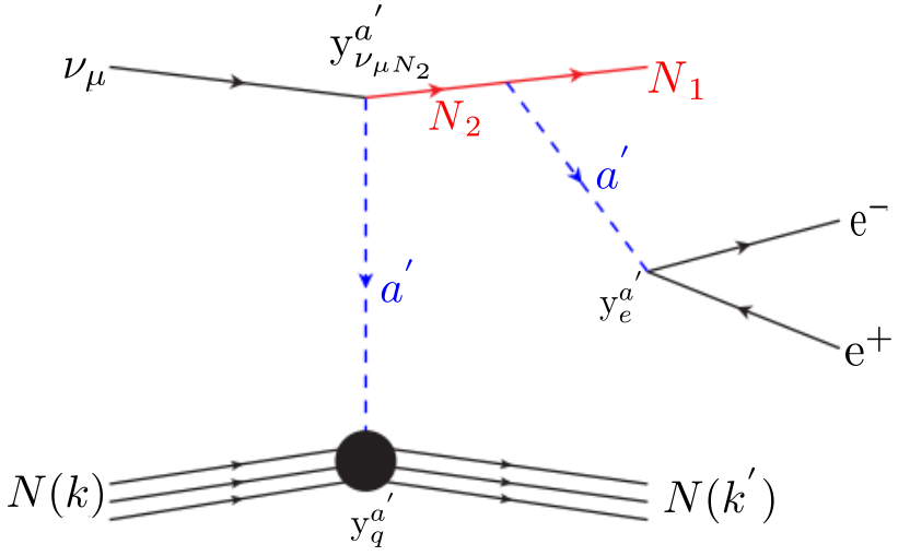
Figure 1: Feynman diagram of the scattering process involving $a^{\prime}$ which leads to the excess in MB and LSND.

3 The interaction in MB and LSND

The Feynman diagram of the process that occurs in MB and LSND in our model, leading to an electron-like signal, is shown in figure 1. The heavy neutral lepton $N_{2}$ is generated via the up-scattering of muon-type neutrinos in the beam. Following its production, $N_{2}$ promptly decays into a lighter neutral lepton $N_{1}$ and a light ($17$ MeV) pseudoscalar $a^{\prime}$, which also decays promptly to a collimated $e^{+}e^{-}$ pair and produces the observed visible light signal. The heavy scalar ($H$) and pseudoscalar ($A$) can also mediate the process that occurs between the incoming neutrino and the nucleon at the primary vertex. However, if their contribution dominates, the angular distribution will lose the necessary forward character, with more events crowding the non-forward bins Abdallah et al. (2022). The relative contribution of $a^{\prime}$ and heavy particles ($H,\,A$) depends on the mass of heavy mediators and the mixing angle $\xi$. The contribution of $H$ and $A$ to the MB excess for our chosen benchmark values is less than $5\%$. Increasing (decreasing) the masses of $A,H$ would reduce (increase) this contribution, whereas increasing (decreasing) $\xi$ would decrease (increase) it.

Our numerical calculations employ the cross-section for the interaction and the model outlined in section 2. Fits to LSND and MB, as well as those for a common understanding of all three anomalies, which we take up in a later section) depend crucially on the couplings of $a^{\prime}$ to $u,d$ quarks and to electrons. The quark couplings are then used to obtain effective nucleon couplings.

The Yukawa interaction of $a^{\prime}$ with quarks is given by

$$\mathcal{L}_{a^{\prime}qq}=y^{a^{\prime}}_{q}\,a^{\prime}\bar{q}\,i\gamma_{5}\,q\,.$$ (32)

In our model, when seeking a solution to MB and LSND alone, the $a^{\prime}$ predominantly couples to the first generation of quarks ($u$ and $d$) and has negligible and much smaller couplings to other families. The effective coupling $(F_{N})$ of $a^{\prime}$ to a nucleon $(N)$ can be written as Cheng and Chiang (2012); Arina et al. (2015),

$$F_{N}=\frac{m_{N}}{m_{q}}\,\sum_{q=u,d,s}\Delta_{q}^{(N)}\,\left(y^{a^{\prime}}_{q}-\sum_{q^{\prime}=u,..,t}y^{a^{\prime}}_{q}\frac{\overline{m}}{m_{q^{\prime}}}\right),$$ (33)

where $\Delta_{q}^{(N)}$ are the quark spin components of the nucleon $N$,

$$\frac{1}{\overline{m}}=\frac{1}{m_{u}}+\frac{1}{m_{d}}+\frac{1}{m_{s}},$$ (34)

$\Delta_{u}^{(p)}=0.84$, $\Delta_{d}^{(p)}=-0.44$, $\Delta_{s}^{(p)}=-0.03$, $\Delta_{u}^{(n)}=-0.44$, $\Delta_{d}^{(n)}=0.84$, $\Delta_{s}^{(n)}=-0.03$ Cheng and Chiang (2012). Here $m_{N}$ is the nucleon mass. All the relevant quark masses are taken from Hikasa et al. (2022).

We note that for the carbon nucleus, which is the primary target in MB and LSND, the total spin of the nucleus is zero. Since any pseudoscalar mediated contribution to the coherent production depends on the spin of the target, we need only consider the incoherent production of $N_{2}$ in MB. The total differential cross-section, for the target in MB, ${\it i.e.}$, CH₂, is thus given by

$$\Big{[}\dfrac{d\sigma}{dE_{N_{2}}}\Big{]}_{{\rm CH_{2}}}\!=\!\Big{[}\underbrace{(8F^{2}_{p}\!+\!6F^{2}_{n})}_{\textrm{\footnotesize{{incoherent}}}}\Big{]}\dfrac{d\sigma}{dE_{N_{2}}}.$$

The number of events is given by

$${\rm N}_{\rm{events}}\!=\!\eta\!\!\int\!\!dE_{\nu}dE_{N_{2}}\dfrac{d\Phi^{\rm{\nu}}}{dE_{\nu}}\!\,\dfrac{d\sigma}{dE_{N_{2}}}\!\times\!{\rm BR}(N_{2}\!\rightarrow\!N_{1}a^{\prime}),$$ (35)

$E_{a^{\prime}}$, which represents the visible energy that manifests itself as light subsequent to $a^{\prime}$ decay, $\in[E_{a^{\prime}},E_{a^{\prime}}+\Delta E_{a^{\prime}}]$. Here $\Delta E_{a^{\prime}}$ is essentially the bin size in our plots for the two detectors. $\eta$ encompasses all detector-related information, such as efficiencies, POT, etc., while $\Phi^{\rm{\nu}}$ represents the incoming muon neutrino flux. The calculations for LSND and MB alone are carried out using the benchmark values in table 1, while when trying to obtain a common solution to all three anomalies, we use the benchmarks given in table 2. The quark and neutrino vertex couplings are quite different for the two tables. We note that the LSND and MB fits depend on the product of the effective couplings at the neutrino and nucleon vertex, for given masses of $N_{2}$ and $a^{\prime}$. The resolution of the ATOMKI anomaly demands higher values of $F_{p}$ and $F_{n}$ which translate into higher (lower) values of quark (neutrino vertex) couplings in table 2 compared to table 1.

4 Results for MB and LSND

This section gives our fits for MB and LSND alone using a light 17 MeV pseudoscalar, without any input from the ATOMKI results.

In Figure 2 (top panels) we present the SM backgrounds, the MB data points, and the predictions from our model (depicted by the blue solid line) within each bin. Additionally, the oscillation best fit is represented by the black dashed line. Our fit utilizes the most recent data set for the neutrino mode, corresponding to $18.75\times 10^{20}$ POT Aguilar-Arevalo et al. (2021). The left panel shows $E_{vis}$, the measured visible energy, plotted against the neutrino events. Note that $E_{vis}$ corresponds to $E_{a^{\prime}}$ in our model. Meanwhile, the right panel displays the angular distributions for the emitted light. The fit is conducted using benchmark parameter values outlined in table 1. We have utilized fluxes, efficiencies and other pertinent details from Aguilar-Arevalo et al. (2018b) and the references therein to generate these plots. Excellent fits to the data are achieved for both the angular and the energy distributions. The data points reflect statistical uncertainties only. We have incorporated a systematic uncertainty of $15\%$ in our calculations, and this tolerance is represented by the blue bands in the figures.

In addition to detecting the $2.2$ MeV photon resulting from coincident neutron capture on hydrogen, LSND measures the visible energy stemming from Cerenkov and scintillation light radiated by the electron-like event. Figure 1 shows how this process takes place in the context of our model, via the scattering off a target neutron within the Carbon nucleus. All requisite information concerning fluxes, efficiencies, POT, etc., for LSND has been sourced from Aguilar et al. (2001b) and the references therein.

Figure 2 (bottom-left panel) illustrates our prediction compared to the LSND data for $R_{\gamma}>10$. Here $R_{\gamma}$ is a measure of the likelihood ratio that the observed $2.2$ MeV photon, which signals the presence of an emitted neutron, was correlated rather than accidental. It has been defined by the LSND Collaboration in e.g. Aguilar et al. (2001b). This panel shows the excess events observed and their energy distribution, as well as those resulting from our model employing the same benchmark parameters as are used to generate the MB fit. For this specific $R_{\gamma}$, we obtain 39.4 total excess events from our model, while LSND reports 32 events.

Figure 2 (bottom-right panel) illustrates, for $R_{\gamma}>1$, the angular distribution of light stemming from the observed electron-like final state. The visible energies shown lie within the range $36~{}{\rm MeV}<{\rm E_{vis}}<60$ MeV. The blue shaded region in both panels represents the prediction of our model, juxtaposed with backgrounds and data. For our benchmark values, we get $\chi^{2}/{\rm dof}=2.2$.

$m_{N_{1}}$	$m_{N_{2}}$	$m_{N_{3}}$	$y_{u}^{a^{\prime}}\!\!\times\!\!10^{6}$	$y_{e}^{a^{\prime}}\!\!\times\!\!10^{5}$	$y_{\mu}^{a^{\prime}}\!\!\times\!\!10^{5}$	$M_{H^{\pm}}$	$y_{c}^{a^{\prime}}$	$y_{t}^{a^{\prime}}$
70 MeV	$120$ MeV	$10$ GeV	$4.34$	$2.3$	$1$	305 GeV	0	0
$M_{a^{\prime}}$	$M_{H}$	$\sin\xi$	$y_{d}^{a^{\prime}}\!\!\times\!\!10^{6}$	$y_{\nu_{\mu N_{2}}}^{a^{\prime}}\!\!\times\!\!10^{2}$	$\lambda_{N_{\!12}}^{a^{\prime}}$	$M_{A}$	$y_{s}^{a^{\prime}}$	$y_{b}^{a^{\prime}}$
17 MeV	300 GeV	$0.01$	$4.0$	$3.15$	$0.1$	400 GeV	0	0

Table 1: Benchmark parameter values used to generate the event spectrum in LSND and MB.

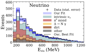
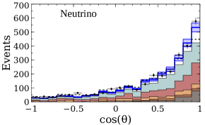
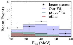
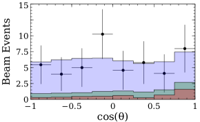
Figure 2: Top panels: These show, for neutrino runs, the MB electron-like events (backgrounds and signal) sourced from Aguilar-Arevalo et al. (2021). They are plotted against the visible energy E_vis (left panel) and the emitted angle of the light (right panel). The blue solid line denotes the prediction of excess events in our model. Bottom panels: These show, for $R_{\gamma}>10$, the energy distribution (left panel) of the LSND data Aguilar et al. (2001b) and, for $R_{\gamma}>1$, the angular distribution (right panel) of the light originating from the electron-like final state. In both panels, the shaded blue region represents our fit, and other shaded regions denote the backgrounds.

5 Derivation of couplings of the pseudoscalar from ATOMKI results

As mentioned above, the ATOMKI collaboration has reported anomalous measurements in the IPC decays of excited ⁸Be Krasznahorkay et al. (2016, 2018), ⁴He Krasznahorkay et al. (2019, 2021) and, more recently, ¹²C Krasznahorkay et al. (2022) nuclei. We note that observations were conducted for two excited states of ⁸Be, specifically ⁸Be(18.15) and ⁸Be(17.64). Similarly, for ⁴He, decays of ⁴He(21.01) and ⁴He(20.21) were studied. The experiment observed unexpected bumps for both the invariant mass and the angular opening of the $e^{+}e^{-}$ pairs with high statistical significance, well above $6\sigma$. As in Ellwanger and Moretti (2016), we derive the values of the couplings of the pseudoscalar to quarks, electrons and nucleons appropriate to a resolution of this anomaly.

Noting that in the SM, the decay of an excited nucleus to a lower state with an equal number of protons and neutrons can happen only via EM processes, the allowed channels are:

• the emission of a real photon, due to the decay of the nucleus.

• The emission of a virtual photon by the nucleus, which decays to an $e^{+}e^{-}$ pair, (Internal Pair Creation (IPC)), i.e.,

  $$p+A\rightarrow N^{*}\rightarrow N+e^{+}+e^{-}\,.$$ (36)

Here $p$ denotes a beam proton and $A$ is a target nucleus. The anomaly appears only in the IPC events. We consider, as an example, the Be case. The experiment used a beam of protons with kinetic energies tuned to the resonance energy of 1.03 MeV, which were made to collide with Li nuclei, in order to form the resonant state ⁸Be^∗. A small percentage of these decayed via ${}^{8}{\!\,\rm Be}^{*}\rightarrow\,^{8}{\!\,\rm Be}+e^{+}e^{-}$. We note that ${}^{8}{\!\,\rm Be}^{*}$ decays to ${}^{7}{\!\,\rm Li}+p$ most of the time, but it also has electromagnetic transitions with branching fractions ${\rm BR}(^{8}{\!\,\rm Be}^{*}\rightarrow\,^{8}{\!\,\rm Be}\,\gamma)\simeq 1.4\times 10^{-5}$ Tilley et al. (2004) and ${\rm BR}(^{8}{\!\,\rm Be}^{*}\rightarrow\,^{8}{\!\,\rm Be}+e^{+}e^{-})\simeq 3.9\times 10^{-3}~{}{\rm BR}(^{8}{\!\,\rm Be}^{*}\rightarrow\,^{8}{\!\,\rm Be}\,\gamma)$ Schlüter et al. (1981); Rose (1949).

The experiment measured both the electron and positron energies, as well as the opening angle of the $e^{+}e^{-}$ pairs, $\theta$, in order to determine the invariant mass ($m_{ee}$) and angular distributions. It did not observe the behaviour predicted by the SM i.e. that the $\theta$ and $m_{ee}$ distributions should fall monotonically. The $\theta$ distribution exhibited a high-statistics bump that peaked at $\theta\simeq 140^{\circ}$ before it returned close to the SM prediction at $\theta\simeq 170^{\circ}$.

Such a bump at large opening angles is expected from the kinematics of a massive particle that is is produced with low velocity in the ${}^{8}{\!\,\rm Be}^{*}$ decay and which then subsequently decays to $e^{+}e^{-}$ pairs. The hypothesis of a new particle $X$ and the two-step decay ${\rm BR}(^{8}{\!\,\rm Be}^{*}\rightarrow\,^{8}{\!\,\rm Be}+X)$ followed by $X\rightarrow e^{+}e^{-}$ thus emerges as a natural resolution to the anomaly. With the assumption of a fixed background, Krasznahorkay et al. Krasznahorkay et al. (2016) give the best fit mass and branching fraction as

$$M_{X}=16.7\pm 0.35({\rm stat})\pm 0.5({\rm sys})~{}~{}{\rm MeV},$$

$$\frac{{\rm BR}(^{8}{\!\,\rm Be}^{*}\rightarrow\,^{8}{\!\,\rm Be}\,X)\times{\rm BR}(X\rightarrow e^{+}e^{-})}{{\rm BR}(^{8}{\!\,\rm Be}^{*}\rightarrow\,^{8}{\!\,\rm Be}\,\gamma)}= 5.8\times 10^{-6}\,.$$

These values correspond to a statistical significance in excess of $6.8\sigma$. Possible types of particles which may provide candidate solutions of the anomaly are a pseudoscalar, a vector or an axial-vector Barducci and Toni (2023). Assuming parity and angular momentum conservation in the decay, the possibility of $X$ being a real scalar is ruled out. Additionally, very strong coupling constraints based on anomaly cancellations apply to a light vector or axial vector that couples to SM fermions via an additional $U(1)$ Dror et al. (2017a, b, 2019). We have thus chosen to focus on a pseudoscalar as our choice for $X$.

For both the Be excited states, a pseudoscalar, which has intrinsic parity $(-1)$ can be emitted in a state of orbital angular momentum 1 with respect to the ground state ${}^{8}{\!\,\rm Be}$, thus conserving both angular momentum and parity. In the case of ${}^{4}{\rm He}$, however, note that only the decay from the excited state ${}^{4}{\rm He}$ (21.01), which has 0 angular momentum and parity $-1$, will be allowed. Also, we note that for the ¹²C nucleus which has spin 1 and parity $-1$, the pseudoscalar does not allow a solution that conserves both overall parity and angular momentum.

5.1 Couplings of the pseudoscalar to quarks

As shown in the previous section in eqs. (32),(33) can be used to obtain the effective nucleon couplings. The average nucleon coupling ($\bar{h}^{2}_{N}$) of $a^{\prime}$ with the ${}^{8}{\!\,\rm Be}^{*}$ is given by

$$\bar{h}^{2}_{N}\equiv\frac{(F_{p}+F_{n})^{2}}{4}\,.$$ (37)

The next step involves a calculation of the Be decay rates given below, employing nuclear matrix elements, and for this we use results from Ellwanger and Moretti (2016)

$$\frac{{\rm BR}(^{8}{\!\,\rm Be}^{*}\rightarrow\,^{8}{\!\,\rm Be}\,A)}{{\rm BR}(^{8}{\!\,\rm Be}^{*}\rightarrow\,^{8}{\!\,\rm Be}\,\gamma)}=\frac{2\bar{h}^{2}_{N}}{0.16\,\,e^{2}}\,\,\frac{|p_{A}|^{3}}{|p_{\gamma}|^{3}}.$$ (38)

We assume ${\rm BR}(A\rightarrow e^{+}e^{-})=1$ and compare to the experimental value from the ${}^{8}{\!\,\rm Be}$ experiment Krasznahorkay et al. (2016), which is

$$\frac{{\rm BR}(^{8}{\!\,\rm Be}^{*}\rightarrow\,^{8}{\!\,\rm Be}\,A)}{{\rm BR}(^{8}{\!\,\rm Be}^{*}\rightarrow\,^{8}{\!\,\rm Be}\,\gamma)}=5.8\times 10^{-6}\,.$$ (39)

The ratio of momenta depends on the pseudoscalar mass $M_{a^{\prime}}$ which in our case is 17 MeV. This leads to

$$\frac{|p_{A}|^{3}}{|p_{\gamma}|^{3}}\sim 0.045\,.$$ (40)

Solving the above three equations, we get the value of $\bar{h}^{2}_{N}=9.38\times 10^{-7}$. We choose the coupling of $a^{\prime}$ to quarks in table 2 such that we get the desired value of $\bar{h}^{2}_{N}$. The value $F_{p}$ ($F_{n}$) for our benchmark parameters is $-0.00871\,(0.00675)$. The ratio of the absolute values of the effective couplings of $a^{\prime}$ with proton and neutron (i.e., $F_{n}/F_{p}=-0.77$) is an important factor in reproducing the correct energy and angular distributions in LSND and MB.

$m_{N_{1}}$	$m_{N_{2}}$	$m_{N_{3}}$	$y_{u}^{a^{\prime}}\!\!\times\!\!10^{5}$	$y_{e}^{a^{\prime}}\!\!\times\!\!10^{5}$	$y_{\mu}^{a^{\prime}}\!\!\times\!\!10^{5}$	$M_{H^{\pm}}$	$y_{c}^{a^{\prime}}\!\!\times\!\!10^{3}$	$y_{t}^{a^{\prime}}\!\!\times\!\!10^{5}$
70 MeV	$120$ MeV	$10$ GeV	$-5.043$	$2.3$	$1$	305 GeV	6.366	$-1.3$
$M_{a^{\prime}}$	$M_{H}$	$\sin\xi$	$y_{d}^{a^{\prime}}\!\!\times\!\!10^{5}$	$y_{\nu_{\mu N_{2}}}^{a^{\prime}}\!\!\times\!\!10^{4}$	$\lambda_{N_{\!12}}^{a^{\prime}}$	$M_{A}$	$y_{s}^{a^{\prime}}\!\!\times\!\!10^{5}$	$y_{b}^{a^{\prime}}$
17 MeV	300 GeV	$0.01$	$-1.3$	$2.84$	$0.1$	400 GeV	$-1.3$	$0$

Table 2: Benchmark parameters used to generate the event spectrum in LSND, MB and for calculating the ATOMKI. The corresponding doublet sector scalar quartic couplings for this benchmark point (BP) are shown in table 3 in the Appendix B.

5.2 Couplings of the pseudoscalar to the electron

Our calculation above assumes that the branching fraction of the pseudoscalar decay to $e^{+}e^{-}$ pairs is very close to 1. Its total width is

$$\Gamma(a^{\prime})=\frac{(y^{a^{\prime}}_{e})^{2}}{8\pi}\,M_{a^{\prime}}$$ (41)

and its decay length is given by

$$l_{a^{\prime}}=\frac{p_{a^{\prime}}}{M_{a^{\prime}}\Gamma(a^{\prime})}.$$ (42)

The momentum in question can be determined from the energetics of the ATOMKI ⁸Be results, since in that decay ${}^{8}{\rm Be}^{*}\rightarrow{\rm{}^{8}Be}\,\,a^{\prime}$ with $M(^{8}{\rm Be}^{*})-M(^{8}{\rm Be})=18.15$ MeV. The size of the ATOMKI detector requires that the pseudoscalar $a^{\prime}$ decay in about 1 cm. This gives $y^{a^{\prime}}_{e}>8.3\times 10^{-6}$. Our benchmark values in table 2 satisfy the inequality and give the value $\bar{h}^{2}_{N}=9.38\times 10^{-7}$.

6 Combined Results for MB, LSND and ATOMKI

Using the coupling values determined from ATOMKI data in the previous section, we obtain fits to MB and LSND. The fits are identical to those shown in the plots of figure 2, for reasons explained towards the end of section 3, hence we do not display them here. Our numerical calculations employ the cross-section for the process and the model outlined in section 3. Fits to LSND and MB, as well as the result of ATOMKI, depend crucially on the couplings of $a^{\prime}$ to nucleons and the electron. Benchmark values for these couplings, shown in table 2, are obtained from those required to obtain the ATOMKI result in section 5, and are then fed into the fitting procedure for MB and LSND with other detector specific inputs. Note that the quark couplings to $a^{\prime}$ are significantly different, and higher, than those required to fit MB and LSND alone.

The fits shown in figure 2 are representative, and it is useful to obtain some feeling for the allowed solution space when one considers the three anomalies together. Since obtaining this space is significantly affected by bounds from charged kaon decays, we have relegated its discussion to the next section, which is dedicated to constraints.

7 Constraints

This section examines constraints on our model from flavour changing meson decays, collider physics, vacuum stability, and electroweak precision data.

7.1 Constraints on a light (17 MeV) pseudoscalar

A singlet $17$ MeV pseudoscalar particle is subject to constraints from many sources. For instance, since in our model it predominantly decays to an $e^{+}e^{-}$ pair, it is subject to some of the constraints from searches for axions or axion-like particles, such as those summarized in Dolan et al. (2015); Andreas et al. (2010); Essig et al. (2010); Pro (2012); Döbrich et al. (2016); Liu et al. (2021). However, we note that $a^{\prime}$ in our model obtains its couplings to fermions via mixing with the Yukawa couplings of the heavier pseudoscalar $A$ belonging to the second Higgs doublet. These couplings do not follow the usual mass-dependence of the SM Yukawa couplings, and are at present unconstrained in many cases, especially for the heavier fermions. This weakens the direct applicability of some of the axion and axion-like bounds. A discussion of many of the other constraints on a $17$ MeV singlet scalar with couplings in the range required to fit MB and LSND alone is given in Ref. Abdallah et al. (2021). Of special relevance among these are bounds from the electron beam dump experiments E137 Bjorken et al. (1988), E141 Riordan et al. (1987), ORSAY Davier and Nguyen Ngoc (1989) and NA64 Banerjee et al. (2018). While our BP is not in violation of these at present, a more thorough mapping of the allowed regions would be worthwhile.

Charged kaon decay constraint and the sample solution space:

A potentially important class of constraints arises from flavour-violating meson decays, see e.g. Dolan et al. (2015). We note that in any heavy meson decay that involves $u,d$ quarks, one can radiate an $a^{\prime}$ which would promptly decay to an $e^{+}e^{-}$ pair via the diagonal couplings between it and the quarks. While off-diagonal flavour changing couplings in our model are arbitrarily small, the first generation diagonal quark couplings to the scalars in our model are fixed by the requirements of fitting the ATOMKI, LSND and MB data, and are approximately $\mathcal{O}(10^{-4})$. For this case, the decay of charged kaons leads to constraints which are especially stringent Dolan et al. (2015); Batell et al. (2019). These decays are dominated by flavour changing penguin processes, and we calculate the decay width and branching ratio ${\rm BR}(K^{+}\rightarrow\pi^{+}a^{\prime}(\pi^{+}+e^{+}e^{-}))$ for our model below.

Prior to that, we note certain caveats which may apply to the two experiments which explored the low mass region ($0-50$ MeV) for $a^{\prime}$, namely a) the $K_{\mu 2}$ experiment E89 Yamazaki et al. (1984) at KEK and b) the BNL-AGS experiment Baker et al. (1987). We note certain aspects which could possibly render the bounds less severe than claimed (for a detailed discussion of their limitations see Alves and Weiner (2018)). Both experiments, when exploring the low mass region relevant to our model, must confront the difficult background from Dalitz pair production, $K^{+}\rightarrow\pi^{+}+(\pi^{0}\rightarrow e^{+}e^{-}\gamma)$. In the case of the KEK experiment, there appears to be significant uncertainty regarding the lower end (in mass) of their sensitivity below 50 MeV, with some papers, for instance Yamazaki showing no sensitivity below this value. Additionally, the method used to infer limits in the range $M_{a^{\prime}}<80$ MeV is considered inappropriate for such a low statistics region, in particular the $\sqrt{N}$ estimation of background error may lead to an overly stringent bound in a Poissonian region Alves and Weiner (2018).

The BNL-AGS experiment has also been criticised for the modelling and subtraction of their background. Their Monte Carlo apparently mis-estimates the Dalitz background contamination by possibly a factor of $\sim 10$ Baker et al. (1987). This has led to questions on their Monte Carlo estimation of the signal acceptance as well Alves and Weiner (2018). Overall, there appears to be significant uncertainty in the bounds on $K^{+}\rightarrow\pi^{+}a^{\prime}$ in the region relevant to our model. Since the experiments are about four decades old, one may conservatively say that exploring this difficult but very interesting region using a recent-day experiment may be worthwhile.

Keeping the above considerations in mind, in finding the sample solution space for common solutions to MB, LSND and ATOMKI shown in figure 4 we have allowed the possibility that BR$(K^{+}\rightarrow\pi^{+}a^{\prime}(\pi^{+}+e^{+}e^{-}))<{\cal O}(10^{-6})$. This is about a factor of   few to an order of magnitude less severe than required by Yamazaki et al. (1984); Baker et al. (1987). Note, however, that in spite of this, figure 4 shows a large region (the right panel) that conforms to the stringent bounds demanded by these experiments.

In addition to not violating kaon decay constraints, the derivation of the sample solution spaces shown in figure 4 must conform to the following conditions, to a reasonable degree of accuracy:
$a)$ the ratio of the absolute values of the effective couplings of $a^{\prime}$ with neutron and proton must be $\frac{F_{N}}{F_{P}}\simeq 0.77$. This requirement stems from fits to the MB and LSND distributions.
$b)$ The average nucleon coupling $\bar{h}^{2}_{N}$, defined in eq. (37) must be $\simeq 9.38\times 10^{-7}$. This requirement, from ATOMKI data, was obtained by solving eqs. (38), (39) and (40).

Noting that while the magnitudes of the couplings $y_{u}^{a^{\prime}}$ and $y_{d}^{a^{\prime}}$ are largely decided by the fitting requirements above, the couplings of the other quarks to $a^{\prime}$ are largely free, but do affect the calculation of the BR of the kaon decay through the $W$-mediated penguin diagrams which dominate its value (figure 3). We seek a solution space in terms of the quark couplings to $a^{\prime}$ and define a tolerance of ($15\%$) in the values defined in $a)$ and $b)$. This is sufficient to lead to good fits to the data in all three experiments.

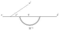
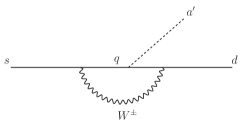
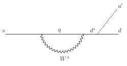
Figure 3: Feynmann diagrams for the flavour-changing transitions such as $s\to da^{\prime}$ involving the exchange of quarks and $W^{\pm}$-bosons in the loop. $q$ stands for up-type quarks $u,c,t$.

The one-loop contribution from flavour-changing diagrams shown in figure 3 are in general divergent. The effective coupling for the interaction $h^{R}_{ds}\,a^{\prime}\,\overline{d}P_{R}s$, where $P_{R}=\frac{1+\gamma_{5}}{2}$ is given by Dolan et al. (2015)

$$h^{R}_{ds} = \sum_{q=u,c,t}\frac{e^{2}\,\left[3\,m_{d}\,m_{s}\,m_{q}^{2}\,y^{a^{\prime}}_{d}-(m_{d}^{2}+2m_{s}^{2})\,m_{q}^{2}\,y^{a^{\prime}}_{s}+2\,m_{s}\,(m_{d}^{2}-m_{s}^{2})\,m_{q}\,y^{a^{\prime}}_{q}\right]}{64\pi^{2}\,m_{W}^{2}\,\sin(\theta_{W})^{2}\,(m_{s}^{2}-m_{d}^{2})}\,V_{qs}V_{qd}^{\ast}\times\frac{1}{\epsilon},$$

where $m_{W}$ is the $W$-boson mass, $\theta_{W}$ is the Weinberg angle and $V_{ij}$ are elements of the CKM matrix. We have used the cutoff regularization replacement $1/\epsilon\rightarrow\log(\Lambda^{2}/m_{t}^{2})$ where $\Lambda$ ($=1$ TeV in our case) is the energy scale at which new physics beyond the Standard Model becomes relevant, and $m_{t}$ is the mass of the top quark. The corresponding expression (upto a sign) for $h^{L}_{ds}$ is obtained by exchanging $s$ and $d$ in eq. (LABEL:eq:1412Ref). The overall effective coupling may then be written as

$$h^{S}_{ds}=\frac{h^{R}_{ds}+h^{L}_{ds}}{2},~{}~{}~{}~{}{\rm and}~{}~{}~{}~{}h^{P}_{ds}=\frac{h^{R}_{ds}-h^{L}_{ds}}{2},$$ (44)

leading to the full pseudoscalar interaction term

$$i\,\overline{s}(h^{S}_{ds}+h^{P}_{ds}\gamma_{5})d.$$ (45)

The coupling $h^{S}_{ds}$ leads to Kaon decay via $K^{\pm}\to\pi^{\pm}a^{\prime}$. Note that the part of the coupling proportional to $h^{P}_{ds}\,\gamma_{5}$ does not contribute to this decay Deshpande et al. (2006). Finally, the partial decay width is given by Deshpande et al. (2006); Dolan et al. (2015)

$$\Gamma(K^{+}\rightarrow\pi^{+}a^{\prime})=\frac{1}{16\pi\,m_{K^{+}}^{3}}\lambda^{1/2}(m_{K^{+}}^{2},m_{\pi^{+}}^{2},M_{a^{\prime}}^{2})\left(\frac{m_{K^{+}}^{2}-m_{\pi^{+}}^{2}}{m_{s}-m_{d}}\right)^{2}|h^{S}_{ds}|^{2}\,,$$ (46)

where the function $\lambda(a,b,c)=(a-b-c)^{2}-4\,b\,c$, $m_{K^{\pm}}$ is the mass of the kaon and $m_{\pi^{\pm}}$ is the mass of the pion.

For our BP in table 2, this leads to ${\rm BR}(K^{\pm}\to\pi^{\pm}a^{\prime})$=$6.13\times 10^{-7}$. The Yukawa couplings are then varied in accordance with the tolerance mentioned above to explore a larger region of parameter space that can simultaneously explain the MB, LSND, and ATOMKI data while remaining consistent with current kaon decay constraints Dolan et al. (2015); Batell et al. (2019). There are six independent couplings, allowing for various solutions. Our aim is to provide a representative sample of points, rather than undertake a full exploration of the allowed space. Thus, for simplicity, we set $y^{a^{\prime}}_{d}=y^{a^{\prime}}_{s}=y^{a^{\prime}}_{t}=y^{a^{\prime}}_{d,s,t}$ and vary $y^{a^{\prime}}_{d,s,t}$, $y^{a^{\prime}}_{u}$ and $y^{a^{\prime}}_{c}$, showing the allowed region. We also choose $y^{a^{\prime}}_{b}=0$ to avoid constraints from the $\Gamma(B^{\pm}\to K^{\pm}a^{\prime})$ decay using a similar loop decay. In figure 4, the left plot shows BR$(K^{\pm}\to\pi^{\pm}a^{\prime})$ $<10^{-5}$, while the right one shows BR$(K^{\pm}\to\pi^{\pm}a^{\prime})$ $<10^{-6}$. The color shading indicates the variation of the charm coupling (depicted by the bar on the right side). These sample plots illustrate that a large region of parameter space can accommodate the MB, LSND, and ATOMKI data while being consistent with constraints coming from the rare meson decay.

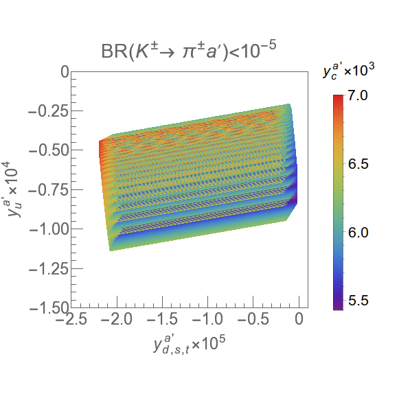
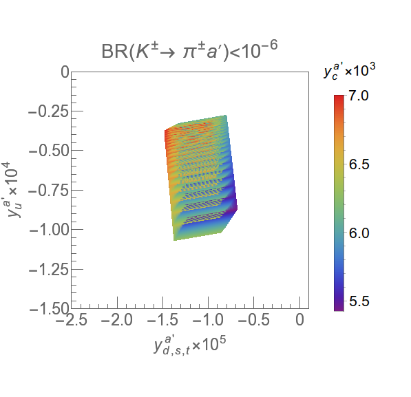
Figure 4: The allowed region in the $y^{a^{\prime}}_{d,s,t}-y^{a^{\prime}}_{u}$ plane (with $y^{a^{\prime}}_{d}=y^{a^{\prime}}_{s}=y^{a^{\prime}}_{t}=y^{a^{\prime}}_{d,s,t}$). $\frac{F_{N}}{F_{P}}$=$-0.77$ $\pm 0.1155$ and $\bar{h}^{2}_{N}\equiv$ $\frac{(F_{p}+F_{n})^{2}}{4}$ = $(9.38\pm 1.407)$ $\times 10^{-7}$. The left plot gives ${\rm BR}(K^{\pm}\to\pi^{\pm}a^{\prime})$ $<10^{-5}$, while the right one maintains ${\rm BR}(K^{\pm}\to\pi^{\pm}a^{\prime})$ $<10^{-6}$. Here we have chosen $y^{a^{\prime}}_{b}$ $=0$, and get BR$(B^{\pm}\to K^{\pm}a^{\prime})$ $<5.2\times 10^{-7}$.

7.2 Constraints from the $Z$ decay width

The LEP experiments measured the $Z$ boson decay width to be $\Gamma(Z\to{\rm All})=2.4952\pm 0.0023$ GeV Workman et al. (2022). Hence, any new physics contribution to this width should lie within $1\sigma$ of the observed central value.

We thus calculate the contributions to $\Gamma(Z)$ in our model. The $CP$-odd scalar $A$ and $CP$-even scalar $H$ masses are heavy and for the purpose of this calculation we take them to be around $\sim 300$ GeV, as shown in table 1 and 2. Thus, while the two-body decay process $Z\to AH$ is kinematically forbidden, a four-body decay to SM fermions mediated by these heavy scalars via their Yukawa couplings is possible. Similarly $Z\to a^{\prime}H$ is also kinematically forbidden as $M_{Z}<M_{a^{\prime}}+M_{H}$ (with $M_{a^{\prime}}=17$ MeV for our BP). However, the three body decay $Z\rightarrow a^{\prime}H^{*}\rightarrow a^{\prime}f\bar{f}$ is still possible, again via Yukawa couplings of $H$. Note that the Yukawa couplings of $H,A$ in our model are small, as can be seen from the benchmark values in table 2 above. Both the 3-body and 4-body decay widths suffer suppression from heavy mediator masses in the propagator and also from phase space suppression. The 3-body decay width is further reduced by the tiny mixing angle $\sin\xi$. Thus, any correction to the total width should be small. We have checked this by calculating both the three-body and four-body decay widths for our BP. The three-body process yields $\Gamma(Z\to a^{\prime}\,\bar{f}\,f)\approx 0.001$ MeV, while the four-body decay yields $\Gamma(Z\to 2\,\bar{f}\,2\,f)\lesssim 10^{-6}$ MeV. Hence, these corrections to the $Z$ width lie comfortably within the presently allowed range.

7.3 Higgs decay width constraints

The channel ($h\rightarrow a^{\prime}a^{\prime}$ with $M_{a^{\prime}}=17$ MeV) can alter the total decay width of the SM Higgs. This partial decay width Gunion et al. is given by

$$\Gamma(h\to a^{\prime}a^{\prime}) = \frac{g_{ha^{\prime}a^{\prime}}^{2}}{32\pi M_{h}}\,\,\left(1-4\,\frac{M_{a^{\prime}}^{2}}{M_{h}^{2}}\right)^{\frac{1}{2}}.$$ (47)

The coupling strength $g_{ha^{\prime}a^{\prime}}$ is dependent on several factors, including $\lambda^{\prime}_{3},\sin\xi$, SM VEV $v$ and scalar masses. Detailed expressions for these dependencies can be found in eq. (A). Measurements by CMS and ATLAS have put bounds on the Higgs total decay width of $3.2^{+2.4}_{-1.7}$ MeV Tumasyan et al. (2022a) and $4.5^{+3.3}_{-2.4}$ MeV Aad et al. (2023b), respectively. Given the large error bars, however, stronger bounds result from the $h\rightarrow a^{\prime}a^{\prime}$ branching ratio. In our model, the 17 MeV $a^{\prime}$ will promptly decay to $e^{+}e^{-}$ with a decay length of about one centimeter, a requirement that primarily stems from MB and LSND. For decay lengths in the range $\mathcal{O}(10^{-1}-10^{3}$ cm), constraints on ${\rm BR}(h\rightarrow a^{\prime}a^{\prime}\rightarrow 2e^{+}\,2e^{-})$ can be derived from the CMS search for long-lived particles decaying to leptons Tumasyan et al. (2022b). This analysis bounds ${\rm BR}(h\rightarrow a^{\prime}a^{\prime})<10^{-4}$ for $M_{a^{\prime}}=30$ and 50 GeV with a decay length of $\mathcal{O}(1$ cm). Although our $a^{\prime}$ is much lighter than the $a^{\prime}$ masses assumed by CMS, we conservatively choose our BP in such a way that this bound on ${\rm BR}(h\rightarrow a^{\prime}a^{\prime})$ is satisfied. We have shown the acceptable region in the $\sin\xi-\lambda_{3}^{\prime}$ plane in figure 5.

Figure 5: The region of the parameter space in the $\sin\xi-\lambda^{{}^{\prime}}_{3}$ plane for which the branching ratio ${\rm BR}(h\to a^{\prime}a^{\prime})<10^{-4}$ of $\Gamma_{\rm SM}^{h}$.

7.4 LHC signal strength constraints

In a model such as the one presented in this paper, with one (or more) additional $CP$-even scalar(s), the tree-level couplings of the SM Higgs-like scalar $h$ to SM fermions and gauge bosons are modified due to mixing. However, since we are working in the alignment limit, the mixing between the observed 125 GeV Higgs and the heavier $CP$-even scalar tends to zero, thus any constraint from the LHC experiments on such a mixing angle is satisfied trivially.

Furthermore, the loop-induced $h\rightarrow\gamma\gamma$ decay is also affected by the presence of the charged scalars ($H^{\pm}$) of the second $SU(2)$ doublet. Despite its small branching fraction of $\sim 0.2\,\%$ Andersen et al. (2013), the $h\to\gamma\gamma$ decay channel provides a clean final-state, leading to a signature that is distinct and easily recognizable against the SM background. Hence, this channel provides stringent constraints in the $g_{hH^{+}H^{-}}-M_{H^{\pm}}$ plane, where $g_{hH^{+}H^{-}}$ is the coupling of the SM-like Higgs boson with $H^{\pm}$, and in our model is equal to $\lambda_{3}v$.

The Higgs to di-photon signal strength, under the narrow width approximation, can be expressed as follows Djouadi (2008),

$$\mu_{\gamma\gamma}=\,\frac{\sigma(gg\rightarrow h)_{\rm BSM}}{\sigma(gg\rightarrow h)_{\rm SM}}\,\frac{{\rm BR}(h\rightarrow\gamma\gamma)_{\rm BSM}}{{\rm BR}(h\rightarrow\gamma\gamma)_{\rm SM}}.$$ (48)

In our model, this formula reduces to

$$\mu_{\gamma\gamma}\approx\frac{\Gamma(h\rightarrow\gamma\gamma)_{\rm BSM}}{\Gamma(h\rightarrow\gamma\gamma)_{\rm SM}}.$$ (49)

At one-loop level, the physical charged Higges $H^{\pm}$ add an extra contribution to the decay width $\Gamma(h\rightarrow\gamma\gamma)_{\rm BSM}$,

$$\Gamma(h\rightarrow\gamma\gamma)_{\rm BSM}=\frac{\alpha^{2}M_{h}^{3}}{256\pi^{3}v^{2}}\Big{|}Q^{2}_{H^{\pm}}\,\frac{v\,g_{hH^{+}H^{-}}}{2M^{2}_{H^{\pm}}}\,F_{0}(\tau_{H^{\pm}})+C_{\rm SM}\Big{|},$$ (50)

where $C_{\rm SM}$ is the contribution from SM particles,

$$C_{\rm SM}=\sum_{f}N_{f}^{c}Q_{f}^{2}y_{f}F_{1/2}(\tau_{f})+y_{W}F_{1}(\tau_{W})$$

with $\tau_{x}=\frac{M_{h}^{2}}{4M_{x}^{2}}$. $Q$ stands for the electric charge of particles, and $N_{f}^{c}$ denotes the color factor. The loop functions $F_{(0,1/2,1)}(\tau)$ are defined in Appendix B, which also contains other calculational details.

The relevant coupling strength of $H^{\pm}$ to $h$ at the tree level is given by, $g_{hH^{+}H^{-}}=\lambda_{3}v=\,(2(M_{H^{\pm}}^{2}-M_{H}^{2})+v^{2}\lambda_{L})\,/\,v$, where $\lambda_{L}=\lambda_{3}+\lambda_{4}+\lambda_{5}$. When the mass gap between charged and $CP$-even scalar fields is large, the coupling $\lambda_{3}$, denoted as $g_{hH^{+}H^{-}}/v$, also becomes large. Consequently, this increase in coupling strength can potentially lead to violations of the observed Higgs to di-photon signal strength. It could also affect unitarity constraints, which we will discuss later. With a coupling strength of $\lambda_{L}=\mathcal{O}(0.01)$ and a relatively smaller mass gap between $M_{H^{\pm}}$ and $M_{H}$, the parameter $\lambda_{3}$ decreases. These choices of input parameters make our model consistent with the $1\sigma$ range of the $h\rightarrow\gamma\gamma$ data. We note that the quartic couplings $\lambda_{3}^{\prime}$ and $\lambda_{L}$ (which includes $\lambda_{3,4,5}$) also influence the Higgs decay width via ${\rm BR}(h\to a^{\prime}a^{\prime})$. This can change the factor $\frac{\Gamma_{\rm SM}^{\rm Total}}{\Gamma_{\rm BSM}^{\rm Total}}$, and hence, $\frac{{\rm BR}(h\rightarrow\gamma\gamma)_{\rm BSM}}{{\rm BR}(h\rightarrow\gamma\gamma)_{\rm SM}}$. In our calculation, we choose ${\rm BR}(h\to a^{\prime}a^{\prime})<10^{-4}$, hence the effect is negligibly small as $\frac{\Gamma_{\rm SM}^{\rm Total}}{\Gamma_{\rm BSM}^{\rm Total}}\approx 1$. However, $\lambda_{3,4,5}$ also face significant constraints from stability and unitarity considerations, which we will discuss in the following subsections.

7.5 Vacuum stability

The requirement that the electroweak vacuum be bounded from below implies that the scalar potential does not tend towards negative infinity along any direction of the scalar field Branco et al. (2012). When the field strengths approach infinity, the quartic terms in the scalar potential dominate. From Chakrabortty et al. (2014); Khan (2022), the conditions which bound our scalar potential from below are

$$\lambda_{1}\geq 0,\lambda_{2}\geq 0,\lambda_{2}^{\prime}\geq 0,\,\lambda_{3}+\lambda_{4}-|\lambda_{5}|>-\sqrt{\lambda_{1}\lambda_{2}}$$

$$\lambda_{3}^{\prime}>-\sqrt{2\,\lambda_{1}\lambda_{2}^{\prime}},\,\lambda_{3}>-\sqrt{\lambda_{1}\lambda_{2}},\,\lambda_{4}^{\prime}>-\sqrt{2\,\lambda_{1}\lambda_{2}^{\prime}}$$ (51)

$$\lambda_{3}+\lambda_{4}>-\sqrt{\lambda_{1}\lambda_{2}}.$$

Above conditions are valid when $\lambda_{6}=\lambda_{7}=\lambda_{5}^{\prime}=0$. The alignment limit demands $\lambda_{6}\rightarrow 0$. For simplicity, we assume $\lambda_{6}=\lambda_{7}=\lambda_{5}^{\prime}=0$, which does not affect the phenomenology of the model considered in this paper.

The quartic couplings $\lambda_{3,4,5}$ and $\lambda^{\prime}_{3,4}$ impose limits on the masses and mixing angles of the scalar sector of the model, particularly affecting the mass differences. For large positive values of $\lambda_{2}$ and $\lambda^{\prime}_{2}$, these bounds can be relaxed. However, large $\lambda$ values may lead to violation of unitarity bounds, which we discuss below. Vacuum stability can also lead to strong bounds on Yukawa couplings since they contribute negatively to the beta function of scalar quartic couplings Khan and Rakshit (2014, 2015); Khan (2022). These considerations are not relevant, however, for the tiny Yukawa couplings considered in our model.

7.6 Unitarity

A set of upper bounds on quartic couplings ($\lambda$’s) of the scalar potential can be imposed by the unitarity of the scattering matrix ($S$-matrix). One can derive the $S$-matrix from various $2\rightarrow 2$ scattering processes involving gauge bosons, scalar particles, and interactions between gauge and scalar bosons. While deriving the $S$-matrix, one approximates the scatterings involving longitudinal gauge bosons by Goldstone bosons in the high energy limit by using the Goldstone-boson equivalence theorem Kanemura et al. (1993); Arhrib (2000). In this limit, scatterings are dominated by four-scalar contact interactions. The procedure for obtaining unitarity bounds is described in Appendix C. Our model has three sub-S-matrices, and the corresponding eigenvalues are as follows.

$$\frac{1}{2}\left(\lambda_{3}-2\lambda_{4}\right),\frac{1}{2}\left(\lambda_{3}-2\lambda_{5}\right),\frac{\lambda_{3}}{2}+\lambda_{4},\frac{\lambda_{3}}{2}+\lambda_{5},\,2\lambda_{2}^{\prime},\frac{1}{4}\left(\lambda_{3}+\lambda_{4}-3\lambda_{5}\right),\lambda_{3}+\lambda_{4}-\frac{\lambda_{5}}{2},$$

$$\frac{1}{4}\left(\lambda_{1}+\lambda_{2}\pm\sqrt{\lambda_{1}^{2}-2\lambda_{2}\lambda_{1}+\lambda_{2}^{2}+16\lambda_{4}^{2}}\right),~{}\frac{1}{4}\left(\lambda_{1}+\lambda_{2}\pm\sqrt{\lambda_{1}^{2}-2\lambda_{2}\lambda_{1}+\lambda_{2}^{2}+16\lambda_{5}^{2}}\right),$$

$$\frac{1}{4}\left(\lambda_{3}^{\prime}+\lambda_{4}^{\prime}\pm\sqrt{\left(\lambda_{3}^{\prime}\right){}^{2}-2\lambda_{4}^{\prime}\lambda_{3}^{\prime}+\left(\lambda_{4}^{\prime}\right){}^{2}+4\left(\lambda_{5}^{\prime}\right){}^{2}}\right),~{}\frac{1}{2}\left(\lambda_{1}+\lambda_{2}\pm\sqrt{\left(\lambda_{1}-\lambda_{2}\right){}^{2}+4\lambda_{4}^{2}}\right),$$

$$\frac{1}{2}\left(3\lambda_{1}+3\lambda_{2}\pm\sqrt{9\left(\lambda_{1}-\lambda_{2}\right){}^{2}+4\left(2\lambda_{3}+\lambda_{4}\right){}^{2}}\right),~{}\frac{1}{2}\left(\lambda_{1}+\lambda_{2}\pm\sqrt{\left(\lambda_{1}-\lambda_{2}\right){}^{2}+4\lambda_{5}^{2}}\right),$$ (52)

$$\frac{1}{8}\left(5\lambda_{3}+5\lambda_{4}+7\lambda_{5}\pm\sqrt{9\lambda_{3}^{2}+18\left(\lambda_{4}-\lambda_{5}\right)\lambda_{3}+73\lambda_{4}^{2}+73\lambda_{5}^{2}+110\lambda_{4}\lambda_{5}}\right),$$

$$\frac{1}{8}\left(\lambda_{3}^{\prime}+\lambda_{4}^{\prime}\pm\sqrt{\left(\lambda_{3}^{\prime}-\lambda_{4}^{\prime}\right){}^{2}+16\left(\lambda_{5}^{\prime}\right){}^{2}}\right)$$

Unitarity demands that the eigenvalues of the $S$-matrix must remain below $8\pi$, ensuring the model’s consistency and validity at extreme energy scales. The results from unitarity considerations for our model are shown in figure 6.

7.7 Constraints from electroweak precision experiments

New physics phenomena beyond the scale of $W$ and $Z$ masses can significantly influence electroweak precision bounds. If such physics contributes dominantly via virtual loops to precision observables, its effects can be parametrized by three-gauge boson self-energy parameters called the oblique parameters. They were introduced and extensively investigated by Peskin and Takeuchi Peskin and Takeuchi (1992), Altarelli et al. Altarelli et al. (1993), and Baak et al. Baak et al. (2014) and are denoted by $S$, $T$, and $U$. The $S(S+U)$ parameter describes new physics contributions to neutral (charged) current processes at different energy scales. The T parameter quantifies differences between the neutral and charged weak currents. The $U$ parameter primarily reflects variations in the mass and width of the $W$-boson. Its contribution is small and subdominant for most new physics cases Baak et al. (2012); Arhrib et al. (2012); Barbieri et al. (2006), including the model presented here, and we neglect it in our following calculations. All the relevant contributions to the oblique parameters in our model arise from the scalars in the second Higgs doublet, while the singlet scalar contributions are negligible. One may then write

$$S=S_{\rm SM}+\Delta S_{\rm SD},~{}T=T_{\rm SM}+\Delta T_{\rm SD},~{}U=U_{\rm SM}+\Delta U_{\rm SD}.$$

The notation SD denotes scalar doublet contributions, which, with $\sin\xi\sim 0$, can be expressed as Arhrib et al. (2012); Barbieri et al. (2006),

$$\Delta S_{\rm SD} = \frac{1}{2\pi}\Big{[}\frac{1}{6}\ln\frac{M_{H}^{2}}{M_{H^{\pm}}^{2}}-\frac{5}{36}+\frac{M_{H}^{2}M_{A}^{2}}{3(M_{A}^{2}-M_{H}^{2})^{2}}+\frac{M_{A}^{4}(M_{A}^{2}-3M_{H}^{2})}{6(M_{A}^{2}-M_{H}^{2})^{3}}\ln\frac{M_{A}^{2}}{M_{H}^{2}}\Big{]},$$ (53)

$$\Delta T_{\rm SD} = \frac{1}{32\pi^{2}\alpha v^{2}}\Big{[}F(M^{2}_{H^{\pm}},M^{2}_{H})+F(M^{2}_{H^{\pm}},M_{A}^{2})-F(M_{A}^{2},M^{2}_{H})\Big{]}.$$ (54)

The two-argument loop function $F$ above is given by

$$F(x,y)=\begin{cases}\frac{x+y}{2}-\frac{xy}{x-y}\ln(\frac{x}{y})&{x\neq y}\\ 0&{x=y}\end{cases}\,.$$

We now constrain the new parameters by using the next-to-next-to-leading order (NNLO) global electroweak fit results obtained by the Gfitter group Haller et al. (2018). Their study yields significant restrictions on the parameter space. The relevant constraints extracted from the fit at a confidence level of $95\%$ are Haller et al. (2018)

$$\Delta S_{\rm SD}<0.04\pm 0.11, \Delta T_{\rm SD}<0.09\pm 0.14, \Delta U_{\rm SD}<-0.02\pm 0.11\,.$$

The contour plots in figure 6 show the permissible area for certain parameters. We have generated these plots by fixing $M_{H}=300$ GeV and varying the masses of $A$ and $H^{\pm}$. We also assume the quartic coupling $\lambda_{2}=0.2$ and from the SM we have $\lambda_{1}=\frac{M_{h}^{2}}{2v^{2}}$. We also set $\lambda_{L}=\lambda_{3}+\lambda_{4}+\lambda_{5}=0.01$ for this analysis. The bounds could vary for different choices of $\lambda_{2}$ and $\lambda_{L}$. Within the plot, the space between the blue dashed lines represents the $1\sigma$ range of the $T$-parameter, while the area between the red dashed lines signifies the $1\sigma$ range of the $S$-parameter. The region to the left of the green line indicates adherence to unitarity constraints. The entire area, above and to the right of the solid red lines, in the $(M_{H^{\pm}}-M_{H})-(M_{A}-M_{H})$ plane is allowed by stability considerations. Notably, the most rigorous constraint arises from the Higgs di-photon signal strength data, shown as the region between the two magenta lines. The hatched area in figure 6 is allowed after considering all constraints. Our chosen benchmark point of table 1 and 2 is shown by the red star.

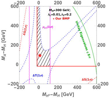
Figure 6: The contour plot shows the allowed region from $i)$ the $S$ and $T$ parameters, $ii)$ stability and $iii)$ unitarity considerations. The allowed region from the Higgs di-photon signal strength data is shown between the magenta lines. For our BP, the most stringent unitarity bound (green line) comes from the eigenvalue: $\frac{3}{2}(\lambda_{1}+\lambda_{2})+$ $\frac{1}{2}\sqrt{}\{9(\lambda_{1}-\lambda_{2})^{2}+$ $4(2\lambda_{3}+\lambda_{4})^{2}\}$ $\leq 8\pi$. The red horizontal (solid red) line is the stability bound came from $\lambda_{3}+\lambda_{4}-|\lambda_{5}|\geq$ $-\sqrt{\lambda_{1}\lambda_{2}}$, whereas the vertical (solid red) line originates from $\lambda_{3}\geq$ $-\sqrt{\lambda_{1}\lambda_{2}}$. The hatched region is what is allowed after considering all constraints. The red $``star"$ mark is our BP corresponding to table 1 and 2.

7.8 Bounds on heavy Higgs masses from LHC searches

Present LHC searches can tightly constrain the singlet and doublet scalar masses via their couplings to the SM fermions. Yukawa couplings relevant to their production and decay are denoted by $\overline{X}$s in eq. (15).

For our choice of the benchmark point, as outlined in Table 2, the heavy $CP$-even (odd) scalar, $H\,(A)$, almost entirely decays to $c\bar{c}$. These decays of $H$ and $A$ will manifest as resonant di-jet signals at the LHC. However, in all the resonant di-jet analyses performed by the LHC collaborations, none go down to 300 GeV mass due to large SM backgrounds. The 2016 CMS analysis is the closest but goes down to the di-jet invariant mass of 500 GeV only Khachatryan et al. (2016). Hence, our benchmark point remains unconstrained from resonant di-jet bounds from the LHC. We also checked that for our benchmark point, the production cross-section of the $p\bar{p}\rightarrow H/A\rightarrow jj$ process at the Tevatron is well below the resonant di-jet cross-sections probed by CDF Aaltonen et al. (2009).

Similarly, the heavy charged scalar, $H^{+}\,(H^{-})$, decays to $c\bar{s}$ ($s\bar{c}$) only. Hence, our values for charged scalar masses $M_{H^{\pm}}$ are consistent with limits obtained from processes such as $pp\to H^{\pm}t\bar{b}(b\bar{t})$, $H^{\pm}\to t\bar{b}(b\bar{t})$ Aad et al. (2021) at the LHC. The heavy Higgs bosons belonging to a $SU(2)$ doublet can also be produced at the LHC by vector boson fusion (VBF) processes followed by their decay into weak gauge bosons. The bounds from these processes are quite strong Sirunyan et al. (2020). However, these bounds are not relevant for us since the heavy Higgs bosons in our model can not be produced by VBF processes as the VEV of the second Higgs doublet is zero.

8 Anomalous magnetic moments of the electron and muon

Since the interaction of $a^{\prime}$ with electrons plays a significant role in our explanation of the three low-energy anomalies which are the subject of this work, it is important to calculate the effect this may have on $a_{e}$. Currently there are discrepancies between the SM prediction and the experimentally observed value of this parameter. The latest experimental measurement of $a_{e}^{\text{Exp}}$ gives the value $115~{}965~{}2180.73\times 10^{-12}$ Hanneke et al. (2008). The theoretical SM estimation of $a_{e}$ Aoyama et al. (2012a, 2018), however, depends on the experimentally measured value of the fine-structure constant, $\alpha$. In recent years, three separate measurements of this parameter have been carried out. Two of these measurements were carried out using the Rubidium (Rb) atomic interferometry Bouchendira et al. (2011); Morel et al. (2020) and one used Caesium (Cs) atomic interferometry Parker et al. (2018). The $\alpha$ measurements from Rb atomic interferometry, carried out in 2010 and 2020, respectively, resulted in $\Delta a_{e}$ = $(-13.0\pm 7.7)\times 10^{-13}$ and $(4.8\pm 3.0)\times 10^{-13}$. These results had significances of $-1.7\sigma$ and $+1.6\sigma$, respectively. The Cs atomic interferometry experiment (2018) led to $\Delta a_{e}$ = $(-8.8\pm 3.6)\times 10^{-13}$ with a significance of $-2.5\sigma$. Thus, depending on the measured value of $\alpha$ that one chooses, the tension between $a_{e}^{\text{Exp}}$ and the prediction of the SM can be either positive or negative.

The one-loop contribution from neutral (pseudo)scalars to $(g_{\ell}-2)$, with $\ell=e,\mu$ is

$$a_{\ell}^{\textrm{one-loop}}=\frac{1}{8\pi^{2}}\sum_{\phi=H,A,a^{\prime}}(y^{\phi}_{\ell})^{2}F_{\phi}\left(\frac{M_{\phi}^{2}}{M_{\ell}^{2}}\right),$$ (55)

where,

$$F_{H}(x)=\int_{0}^{1}dz\frac{(1-z)^{2}(1+z)}{zx+(1-z)^{2}}\,,\qquad\qquad F_{A,a^{\prime}}(x)=-\int_{0}^{1}dz\frac{(1-z)^{3}}{zx+(1-z)^{2}}.$$ (56)

The Barr-Zee two-loop diagram contributions from them Chang et al. (2001); Larios et al. (2001); Ilisie (2015) is

$$a_{\ell}^{\textrm{two-loop}}=\frac{\alpha}{8\pi^{3}}\sum_{\phi=H,A,a^{\prime}}\sum_{f=t,b,\tau}N^{f}_{c}Q_{f}^{2}y_{\ell}^{\phi}y_{f}^{\phi}\frac{M_{\ell}M_{f}}{M_{\phi}^{2}}G_{\phi}\left(\frac{M_{f}^{2}}{M_{\phi}^{2}}\right),$$ (57)

where $N_{c}^{f}$ is the number of colours with $N_{c}^{f}=1(3)$ for leptons (quarks), $Q_{f}$ the electric charge of fermion and

$$G_{H}(x)=\int_{0}^{1}dz\frac{2z(1-z)-1}{z(1-z)-x}\log\frac{z(1-z)}{x}\,,~{}~{}~{}~{}~{}~{}~{}G_{A,a^{\prime}}(x)=\int_{0}^{1}dz\frac{\log\frac{z(1-z)}{x}}{z(1-z)-x}\,.$$ (58)

As mentioned above, $\Delta a_{e}$ could be either positive or negative, hence the role of contributions coming from both one-loop and two-loop levels could be significant. This is because at one-loop, the integrals $F$ become positive (negative) for $CP$-even ($CP$-odd) scalars, as described in eq. (56), while the two-loop integral functions $G$, described in eq. (58), can become either negative or positive for both $CP$-odd and $CP$-even scalars. Thus, a 17 MeV pseudoscalar will always make a negative contribution to $\Delta a_{e}$ at the one-loop level. Since the doublet-like scalars are heavy, their contributions can also remain small at the one-loop level, despite their couplings ($y_{e}^{H,A,H^{\pm}}$) not being $\sin\xi$ suppressed.

At the two-loop level, contributions depend linearly on the product of $y_{\ell}^{\phi}$ and $y_{f}^{\phi}$ (whereas the one-loop contributions depend on $(y_{\ell}^{\phi})^{2}$). Thus, depending on the various sign combinations of these two parameters, the contributions of $CP$-even and $CP$-odd scalars can change signs, as long as they maintain a relative negative sign between them. Using the BP values in table 2, we find that the total (one-loop plus two-loop) contribution to the electron $g-2$ is $\Delta a_{e}\sim-\,{\cal{O}}(10^{-14})$, which is quite small.

Next, we note that the excesses observed by MB, LSND, and ATOMKI can also be accounted for by considering $y_{e}^{a^{\prime}}=1.5\times 10^{-4}$ (i.e., a value one order of magnitude larger than that in table 2), while keeping all other parameters same as table 2. (This change does not violate the constraints outlined in section 6.) Due to this change, the absolute value of the one-loop contribution, given its quadratic dependence on the coupling, will exceed the two-loop correction. One then obtains $\Delta a^{\textrm{one-loop}}_{e}\simeq-1.34\times 10^{-12}$. We note that the two-loop contributions of $M_{A}$, $M_{a^{\prime}}$ and $M_{H}$ offset each other and yield a small positive contribution of $\Delta a^{\textrm{two-loop}}_{e}\simeq 1.11\times 10^{-14}$ for $y_{\tau}^{H/A}=0.3$. This demonstrates that it is possible to align with observations from Rb atomic interferometry (2010) and Cs atomic interferometry (2018). Varying the masses of the $M_{H}$, $M_{A}$ and $\sin\xi$, the two-loop correction can be positive, and of order $10^{-12}$. The negative contribution from the one-loop and the positive contribution from the two-loop being of the same order, can partially offset each other and induce a positive $\Delta a_{e}\sim 10^{-13}$ which is close to the Rb atomic interferometry 2020 result. Thus, in this model it is possible to address both the positive and negative discrepancies of $\Delta a_{e}$ while concurrently explaining the MB, LSND, and ATOMKI excesses, and satisfying all other constraints.

$a_{\mu}$ can receive contributions from a non-zero value of $y_{\mu}^{H,A,a^{\prime}}$. However, there is appreciable uncertainty in the estimation of its theoretical prediction Aoyama et al. (2020, 2012b, 2019); Czarnecki et al. (2003); Gnendiger et al. (2013); Davier et al. (2017); Keshavarzi et al. (2018); Colangelo et al. (2019); Hoferichter et al. (2019); Davier et al. (2020); Keshavarzi et al. (2020a); Kurz et al. (2014); Melnikov and Vainshtein (2004); Masjuan and Sanchez-Puertas (2017); Colangelo et al. (2017); Hoferichter et al. (2018); Gérardin et al. (2019); Bijnens et al. (2019); Colangelo et al. (2020); Blum et al. (2020); Colangelo et al. (2014); Borsanyi et al. (2021); Abi et al. (2021); Bennett et al. (2006); Aguillard et al. (2023). The hadronic vacuum polarization (HVP) contribution to $a_{\mu}$ obtained using dispersion theory, with its value extracted from the precise experimental measurement of the cross-section of the low-energy process ($e^{+}e^{-}\rightarrow$ hadrons) Aoyama et al. (2020); Keshavarzi et al. (2018); Colangelo et al. (2019); Hoferichter et al. (2019); Davier et al. (2020); Keshavarzi et al. (2020a); Kurz et al. (2014); Ignatov et al. (2024a, b); Lees et al. (2012); Ablikim et al. (2016); Anastasi et al. (2018); Masjuan et al. (2024), differs from the lattice-QCD calculation. Thus, the current discrepancy between $a_{\mu}^{\rm SM}$ and $a^{\text{avg(Exp)}}_{\mu}$ can vary between a significance of $5.1\sigma$ to 1.6$\sigma$ depending on one’s choice. In either case, one needs a positive contribution to $\Delta a_{\mu}$ of order $10^{-9}$ from new physics to explain it. In our model, for the choice of $M_{H}$, $M_{A}$, $M_{a^{\prime}}$ and $\sin\xi$ required for our fits to MB and LSND, $\Delta a^{\textrm{one-loop}}_{\mu}$ always remains negative. A positive large $a^{\textrm{two-loop}}_{\mu}$ can be obtained by considering the couplings of the heavy fermion with the scalars to be relatively large. As we discuss in section 5, constraints coming from the study of the kaon decay restrict these couplings and prevent a $\Delta a^{\textrm{two-loop}}_{\mu}$ contribution of order $10^{-9}$. Thus, we always get an overall negative contribution to $\Delta a_{\mu}$. This is small ($\sim-10^{-11}$), since the couplings of the muon with the scalars, being free, can be kept small as in table 2.

9 Tests of the model

Several models proposed to explain the excess in MB lead to the creation of $e^{+}e^{-}$ pairs in the detector. The earliest hints of such pair creation could come from MicroBooNE, a 85 t active volume Liquid Argon Time-Projection (LArT-PC) chamber placed 470 m away from the target. MicroBooNE is part of the Short Baseline Neutrino (SBN) program Acciarri et al. (2015); Machado et al. (2019) at Fermilab, and is fed by its Booster Neutrino Beam (BNB), which provided MB with its flux. MicroBooNE has already conducted important tests to restrict or eliminate SM possibilities of the MB excess Abratenko et al. (2022b, c, d, e). Given its superior particle identification capability, its ongoing search for $e^{+}e^{-}$ pairs as the origin of the MB excess and its capability to measure their invariant mass, it may provide the earliest indications for or against the model proposed here.

Two additional detectors are part of SBN: the ICARUS detector, currently operating with a fiducial mass of 760 t, located 600 m from the BNB target, and the Short-Baseline Near Detector (SBND), with a 112-t active volume at a distance of 110 m. Over the next few years, the three detectors in conjunction have the capability to test various new physics proposals for the excess, including those involving sterile-active oscillations, additional photons, electrons and $e^{+}e^{-}$ pairs.

Several experiments are planned to test the ATOMKI result by studying IPC from nuclear transitions, as the experiment at ATOMKI did. We mention two of them here, and refer the reader to Alves et al. (2023) for a much more extensive discussion. The MEG-II experiment Baldini et al. (2018) at the Paul Scherrer Institute in Switzerland, plans to repeat the ⁷Li$(p,e^{+}e^{-})$ ⁸Be measurement. The PADME experiment Raggi and Kozhuharov (2014) will explore the region $16.4$ MeV $\leq M_{a^{\prime}}\leq 17.4$ MeV in its search for the 17 MeV pseudoscalar. Additionally, the kaon DAR search, planned at the JSNS² experiment Ajimura et al. (2017); Jordan (2020) is in a position to provide a possible test of the proposal presented in this work via its flux of high energy muon neutrinos.

The mass of $a^{\prime}$ lies close to, but outside of, existing bounds from electron beam- dump experiments like E141 Riordan et al. (1987). Hence it is feasible that this region in mass and coupling may be covered in the near future by other experiments like HPS Battaglieri et al. (2015). Finally, we mention an existing experimental hint which could be indicative, i.e., a significant excess in the $10-20$ MeV invariant mass-bin of electron-like FGD1-TPC pairs detected by the T2K ND280 detector, (see figure 11 in Abe et al. (2020)).

10 Discussion and Conclusions

The MB and LSND excesses of electron-like events are long-standing and statistically significant anomalies which have defied attempts to explain them using standard physics, even though stringent checks of backgrounds and systematic errors have been conducted. They may be indicative signals of new physics. Additionally, we note that if one seeks a common new physics solution to MB and LSND, scalar mediators do much better than vector ones. This conclusion follows from a comparative study Abdallah et al. (2022) of the up-scattering cross-section both above and below MB energies.

The ATOMKI experiment on rare nuclear transitions requires a new, 17 MeV mediator to explain the excess seen by it. The possible parity and angular momentum conserving choices are a vector, axial vector or a pseudoscalar, decaying into $e^{+}e^{-}$ pairs to explain the bumps in its data via new physics. Taking cognizance of this, we have presented a two-Higgs doublet model with a dark singlet 17 MeV pseudoscalar ($a^{\prime}$). We first show that independent of ATOMKI, such a model provides very good fits of MB and LSND excesses. It is useful to compare our work in this paper with an earlier attempt with a similar model. It was shown in Abdallah et al. (2021) that a second Higgs doublet with a light $(\sim 750$ MeV) $CP$-even scalar, plus a real, 17 MeV singlet scalar mediator which predominantly decayed to $e^{+}e^{-}$ pairs could provide very good fits to datasets of both MB and LSND. At this point it is relevant to note that the observed angular distribution of MB is an important guide to making choices about the new physics model. This distribution is significantly forward, but also has excess events in angular bins in almost all other directions. In Abdallah et al. (2021), such a distribution was achieved by combining the predominantly coherent and forward events generated by the real 17 MeV scalar with a heavier 750 MeV $CP$-even doublet scalar, where the latter helped populate non-forward bins. In this work, the spin dependant couplings and consequent incoherent scattering of the pseudoscalar $a^{\prime}$ alone help achieve the necessary angular distribution in MB, and allows us to also fit LSND simultaneously. All the scalars of the second doublet stay heavy, with masses well above $M_{W}$ and $M_{Z}$, allowing for a natural hierarchy, because the need for the $CP$-even doublet scalar to have a lower mass ($\sim 750$ MeV) is removed. Table 1 displays representative benchmark couplings necessary to achieve this solution.

We next attempt to use the model to fit ATOMKI in addition to MB and LSND. We first identify the $u,d,e$ couplings of the pseudoscalar required to satisfy the ATOMKI anomaly, and then use these values as inputs for the interaction (shown in figure 2) in MB and LSND, and obtain very good fits of their data, albeit with quark couplings to the $a^{\prime}$ which are considerably higher than in the previous case described above (see table 2). This leads the combined solution to the three anomalies to be in tension with kaon decay experiments Yamazaki et al. (1984); Baker et al. (1987). We discuss reasons which may render these bounds to be less severe than is usually believed, and using them, obtain an acceptable range for the branching ratio relevant to our case, BR$(K^{+}\rightarrow\pi^{+}a^{\prime})$. We then show a sample solution space of quark couplings which satisfies this constraint and provides an acceptable fit to the data of all three experiments.

We compute the contributions to the electron and muon $g-2$ up to two loops. In our scenario, it is possible to explain the currently observed discrepancies in the anomalous magnetic moment of the electron, in addition to addressing the MB, LSND, and ATOMKI excesses, while satisfying all other constraints; however, extending the present model is necessary to explain the observed anomalous magnetic moment of the muon. Finally, we have taken into consideration both collider and non-collider constraints on the model and discussed future tests which may validate or invalidate it.

We conclude with a few general comments:

$a)$ The essential elements of the gauge invariant model presented here are the dark singlet $a^{\prime}$ and the $N_{i}$, which are the sub-GeV ($N_{1},N_{2}$) and GeV-scale ($N_{3}$) neutral leptons. These are directly related to the three low energy anomalies we have made an effort to explain. As in Abdallah et al. (2021), the 17 MeV singlet provides a portal to the dark sector, and the three heavy singlet neutrinos help obtain masses for the SM neutrinos via a see-saw mechanism, yielding mass-squared differences in agreement with global oscillation data. Additionally, two of these three singlet neutrinos participate in the interaction used to explain the MB and LSND excess as shown in figure 1.

$b)$ The heavy sector of the model, ${\it i.e.}$ the second Higgs doublet, is an important but supplementary part of the solution presented here. The role of the doublet in this model is to provide a simple mechanism for the $a^{\prime}$ to obtain its couplings to the SM fermions in a gauge invariant manner, via its mixing with the heavier pseudoscalar $A$. In nature, it is not inconcieveable that this supplementary role is played instead by elements of an extended dark sector interacting feebly with SM particles. Similarly, if realised in nature, it is possible that the 17 MeV singlet scalar is a complex field with both real and pseudoscalar components with couplings appropriate to a joint solution of MB and LSND or to a common resolution of all three anomalies considered here.

$c)$ While the excesses seen by MB and LSND are long standing and have been well scrutinized, our attempt to obtain a common solution for all three anomalies rests on the assumption that the ATOMKI results, which are relatively recent, are a genuine signal of a new physics mediator with mass 17 MeV. Further independent tests are clearly necessary to confirm this. In the near future, these include the MEG-II experiment Baldini et al. (2018) as well as the PADME experiment Raggi and Kozhuharov (2014).

Appendices

Appendix A Important vertices

Vertices that are used in our calculation are shown below:

$$g_{hHH} = i\,\lambda_{L}v,$$

$$g_{hAA} = \frac{i}{2}\left(\frac{\left(M_{a^{\prime}}^{2}-M_{A}^{2}\right)}{v}\sin^{2}2\xi-2\,\lambda^{\prime}_{3}v\sin^{2}\xi-2\left(\lambda_{L}-2\lambda_{5}\right)v\cos^{2}\xi\right),$$

$$g_{hAa^{\prime}} = -\frac{i}{2}\left(\frac{\left(M_{a^{\prime}}^{2}-M_{A}^{2}\right)}{v}\cos 2\xi\,\sin 2\xi+\left(\lambda_{L}-2\lambda_{5}-\lambda^{\prime}_{3}\right)v\sin 2\xi\right),$$ (59)

$$g_{ha^{\prime}a^{\prime}} = -\frac{i}{2}\left(\frac{\left(M_{a^{\prime}}^{2}-M_{A}^{2}\right)}{v}\sin^{2}2\xi+2\lambda^{\prime}_{3}v\cos^{2}\xi+2\left(\lambda_{L}-2\lambda_{5}\right)v\sin^{2}\xi\right),$$

with

$$\lambda_{L} = \lambda_{3}+\lambda_{4}+\lambda_{5},$$

$$\lambda_{3} = \dfrac{1}{v^{2}}(-2M_{H}^{2}+2M_{H^{\pm}}^{2}+v^{2}\lambda_{L}),$$

$$\lambda_{4} = \dfrac{1}{v^{2}}(M_{{A}}^{2}\cos^{2}\xi+M_{a^{\prime}}^{2}\sin^{2}\xi+M_{H}^{2}-2M_{H^{\pm}}^{2}),$$

$$\lambda_{5} = \dfrac{1}{v^{2}}(M_{H}^{2}-\cos^{2}\xi M_{A}^{2}-\sin^{2}\xi M_{a^{\prime}}^{2}).$$

$$g_{Z_{\mu}AH} = \frac{\sqrt{g_{1}^{2}+g_{2}^{2}}}{2}\cos\xi\,(p_{\mu}^{A}-p_{\mu}^{H}),~{}~{}g_{Z_{\mu}a^{\prime}H}=\frac{\sqrt{g_{1}^{2}+g_{2}^{2}}}{2}\sin\xi\,(p_{\mu}^{a^{\prime}}-p_{\mu}^{H})$$

$$g_{W_{\mu}^{\pm}H^{\mp}H} = i\,\,\frac{g_{2}}{2}\,(p_{\mu}^{H^{\pm}}-p_{\mu}^{H}),~{}~{}g_{W_{\mu}^{\pm}H^{\mp}A}=\frac{g_{2}}{2}\,(p_{\mu}^{H^{\pm}}-p_{\mu}^{A}),~{}~{}g_{H^{\pm}H^{\mp}h}=i\,\lambda_{3}\,v\,.$$ (60)

$\lambda_{1}$	$\lambda_{2}$	$\lambda_{L}$	$\lambda_{3}$	$\lambda_{4}$	$\lambda_{5}$	$\lambda_{6}=\lambda_{7}=\lambda_{5}^{\prime}$	$\lambda_{3}^{\prime}$	$\lambda_{4}^{\prime}$
$\frac{M_{h}^{2}}{2v^{2}}\approx 0.13$	$0.2$	$0.01$	$0.109$	$0.553$	$-0.653$	$0$	$0.001$	$0.1$

Table 3: The quartic couplings corresponding to our BP as in table 1 and 2.

Appendix B Higgs di-photon signal strength

Consider the following ratios of the production cross-sections $\sigma(pp\to h)$ and decay widths $h\to\chi$ in the presence and absence of new physics,

$$\frac{\sigma(pp\to h)_{\rm BSM}}{\sigma(pp\to h)_{\rm SM}}~{}~{}~{}~{}~{}~{}{\rm and}~{}~{}~{}~{}~{}~{}\frac{\Gamma(h\to\chi)_{\rm BSM}}{\Gamma(h\to\chi)_{\rm SM}},$$ (61)

where $\chi$ generically stands for the final states $b\bar{b},\,\tau^{-}\tau^{+},\,W^{-}W^{+},\,ZZ,\,Z\gamma$ and $\gamma\gamma$.

The Higgs to di-photon strength, under the narrow width approximation, can be expressed as follows,

$$\mu_{\gamma\gamma}=\,\frac{\sigma(gg\rightarrow h)_{\rm BSM}}{\sigma(gg\rightarrow h)_{\rm SM}}\,\frac{{\rm BR}(h\rightarrow\gamma\gamma)_{\rm BSM}}{{\rm BR}(h\rightarrow\gamma\gamma)_{\rm SM}}.$$ (62)

Here, for our model $\frac{\sigma(gg\rightarrow h)_{\rm BSM}}{\sigma(gg\rightarrow h)_{\rm SM}}=1$, hence

$$\mu_{\gamma\gamma}=\frac{\Gamma_{\rm SM}^{\rm Total}}{\Gamma_{\rm BSM}^{\rm Total}}\,\frac{\Gamma(h\rightarrow\gamma\gamma)_{\rm BSM}}{\Gamma(h\rightarrow\gamma\gamma)_{\rm SM}}.$$ (63)

For the case when the new particle’s mass is greater than $\frac{M_{h}}{2}$ or small ${\rm BR}(h\to a^{\prime}a^{\prime})<10^{-4}$, one can write $\frac{\Gamma_{\rm SM}^{\rm Total}}{\Gamma_{\rm BSM}^{\rm Total}}\approx 1$, hence,

$$\mu_{\gamma\gamma}=\frac{\Gamma(h\rightarrow\gamma\gamma)_{\rm BSM}}{\Gamma(h\rightarrow\gamma\gamma)_{\rm SM}}.$$ (64)

At one-loop level, the physical charged Higges $H^{\pm}$ add an extra contribution to the decay width $\Gamma(h\rightarrow\gamma\gamma)_{\rm BSM}$ Djouadi (2008),

$$\Gamma(h\rightarrow\gamma\gamma)_{\rm BSM}=\frac{\alpha^{2}M_{h}^{3}}{256\pi^{3}v^{2}}\Big{|}Q^{2}_{H^{\pm}}\,\frac{v\,g_{hH^{+}H^{-}}}{2M^{2}_{H^{\pm}}}\,F_{0}(\tau_{H^{\pm}})+C_{\rm SM}\Big{|},$$ (65)

where $C_{\rm SM}$ is the contribution from SM particles,

$$C_{\rm SM}=\sum_{f}N_{f}^{c}Q_{f}^{2}y_{f}F_{1/2}(\tau_{f})+y_{W}F_{1}(\tau_{W}),$$

with $\tau_{x}=\frac{M_{h}^{2}}{4M_{x}^{2}}$. $Q$ stands for the electric charge of particles, and $N_{f}^{c}$ denotes the color factor. The loop functions $F_{(0,1/2,1)}(\tau)$ are defined as Djouadi (2008)

$$F_{0}(\tau) =-[\tau-f(\tau)]\tau^{-2}\,,$$

$$F_{1/2}(\tau) =2[\tau+(\tau-1)f(\tau)]\tau^{-2}\,,$$

$$F_{1}(\tau) =-[2\tau^{2}+3\tau+3(2\tau-1)f(\tau)]\tau^{-2}\,,$$

where

$$f(\tau)=\bigg{\{}\begin{array}[]{ll}(\sin^{-1}\sqrt{\tau})^{2}\,,&\tau\leq 1\\ -{1\over 4}[\ln{1+\sqrt{1-\tau^{-1}}\over 1-\sqrt{1-\tau^{-1}}}-i\pi]^{2}\,,&\tau>1\end{array}\;.$$ (66)

Appendix C Unitarity of $S$-matrices

The scalar quartic couplings in the physical bases, denoted by $h,G^{\pm},G^{0},H,H^{\pm},A,$ and $a^{\prime}$, are intricate functions of the parameters $\lambda$’s and $\xi$. This complexity poses significant challenges when calculating the unitary bounds in these physical bases. An alternative approach involves considering non-physical scalar field bases, namely $H_{1}^{0},G^{\pm},G^{0},H_{2}^{0},H_{2}^{\pm},A_{2}^{0},$ and $A_{3}^{0}$, before Electroweak Symmetry Breaking (EWSB). A crucial insight is that the $S$-matrix, originally expressed in terms of the physical fields, can be transformed into an $S$-matrix for the non-physical fields by employing a unitary transformation Kanemura et al. (1993); Arhrib (2000). This transformation allows for a more tractable analysis of unitarity bounds and facilitates calculations within this framework.

In this scenario, the complete set of non-physical scalar scattering processes can be represented by a $23\times 23$ $S$-matrix. This matrix comprises three distinct submatrices with dimensions $10\times 10$, $7\times 7$, and $6\times 6$, respectively, corresponding to different initial and final states involved in the scattering processes.

The first Scattering matrix $\mathcal{M}_{1}$ to scattering processes with one of the following initial and final states: $\{G^{0}G^{+},A^{0}_{2}G^{+},A^{0}_{3}G^{+},H^{0}_{1}G^{+},H^{0}_{2}G^{+},G^{0}H^{+}_{2},A^{0}_{2}H^{+}_{2},A^{0}_{3}H^{+}_{2},H^{0}_{1}H^{+}_{2},H^{0}_{2}H^{+}_{2}\}$ as,

The sub-scattering matrix $\mathcal{M}_{2}$ corresponds to the following initial and final states: $\{G^{+}G^{-}$,
$H^{+}_{2}H^{-}_{2}$,$\frac{(G^{0})^{2}}{\sqrt{2}}$,$\frac{(A_{2}^{0})^{2}}{\sqrt{2}}$,$\frac{(A_{3}^{0})^{2}}{\sqrt{2}}$,$\frac{(H^{0}_{1})^{2}}{\sqrt{2}}$,$\frac{(H^{0}_{2})^{2}}{\sqrt{2}}\}$

The third Scattering matrix $\mathcal{M}_{3}$ to scattering processes with one of the following initial and final states: $\{G^{+}H^{-}_{2},G^{-}H^{+}_{2},G^{0}A_{2}^{0},G^{0}A_{3}^{0},A_{2}^{0}A_{3}^{0},H^{0}_{1}H^{0}_{2}\}$

References

- Martin (1998) S. P. Martin, Adv. Ser. Direct. High Energy Phys. 18, 1 (1998), arXiv:hep-ph/9709356 .
- Workman et al. (2022) R. L. Workman et al. (Particle Data Group), PTEP 2022, 083C01 (2022).
- Eichten et al. (1983) E. Eichten, K. D. Lane, and M. E. Peskin, Phys. Rev. Lett. 50, 811 (1983).
- Aguilar et al. (2001a) A. Aguilar et al. (LSND), Phys. Rev. D 64, 112007 (2001a), arXiv:hep-ex/0104049 .
- Aguilar-Arevalo et al. (2007) A. A. Aguilar-Arevalo et al. (MiniBooNE), Phys. Rev. Lett. 98, 231801 (2007), arXiv:0704.1500 [hep-ex] .
- Aguilar-Arevalo et al. (2009) A. A. Aguilar-Arevalo et al. (MiniBooNE), Phys. Rev. Lett. 102, 101802 (2009), arXiv:0812.2243 [hep-ex] .
- Aguilar-Arevalo et al. (2013) A. A. Aguilar-Arevalo et al. (MiniBooNE), Phys. Rev. Lett. 110, 161801 (2013), arXiv:1303.2588 [hep-ex] .
- Athanassopoulos et al. (1997) C. Athanassopoulos et al. (LSND), Nucl. Instrum. Meth. A 388, 149 (1997), arXiv:nucl-ex/9605002 .
- Katori (2020) T. Katori (MiniBooNE), in 3rd World Summit on Exploring the Dark Side of the Universe (2020) pp. 139–148, arXiv:2010.06015 [hep-ex] .
- Dasgupta and Kopp (2021) B. Dasgupta and J. Kopp, Phys. Rept. 928, 1 (2021), arXiv:2106.05913 [hep-ph] .
- Brdar and Kopp (2022) V. Brdar and J. Kopp, Phys. Rev. D 105, 115024 (2022), arXiv:2109.08157 [hep-ph] .
- Alvarez-Ruso and Saul-Sala (2021) L. Alvarez-Ruso and E. Saul-Sala, Eur. Phys. J. ST 230, 4373 (2021), arXiv:2111.02504 [hep-ph] .
- Abratenko et al. (2022a) P. Abratenko et al. (MicroBooNE), Phys. Rev. Lett. 128, 111801 (2022a), arXiv:2110.00409 [hep-ex] .
- Krasznahorkay et al. (2016) A. J. Krasznahorkay et al., Phys. Rev. Lett. 116, 042501 (2016), arXiv:1504.01527 [nucl-ex] .
- Krasznahorkay et al. (2019) A. J. Krasznahorkay et al., (2019), arXiv:1910.10459 [nucl-ex] .
- Krasznahorkay et al. (2021) A. J. Krasznahorkay, M. Csatlós, L. Csige, J. Gulyás, A. Krasznahorkay, B. M. Nyakó, I. Rajta, J. Timár, I. Vajda, and N. J. Sas, Phys. Rev. C 104, 044003 (2021), arXiv:2104.10075 [nucl-ex] .
- Krasznahorkay et al. (2022) A. J. Krasznahorkay et al., Phys. Rev. C 106, L061601 (2022), arXiv:2209.10795 [nucl-ex] .
- Anselmann et al. (1995) P. Anselmann et al. (GALLEX), Phys. Lett. B 342, 440 (1995).
- Hampel et al. (1998) W. Hampel et al. (GALLEX), Phys. Lett. B 420, 114 (1998).
- Kaether et al. (2010) F. Kaether, W. Hampel, G. Heusser, J. Kiko, and T. Kirsten, Phys. Lett. B 685, 47 (2010), arXiv:1001.2731 [hep-ex] .
- Abdurashitov et al. (1996) D. N. Abdurashitov et al., Phys. Rev. Lett. 77, 4708 (1996).
- Abdurashitov et al. (1999) J. N. Abdurashitov et al. (SAGE), Phys. Rev. C 59, 2246 (1999), arXiv:hep-ph/9803418 .
- Abdurashitov et al. (2006) J. N. Abdurashitov et al., Phys. Rev. C 73, 045805 (2006), arXiv:nucl-ex/0512041 .
- Abdurashitov et al. (2009) J. N. Abdurashitov et al. (SAGE), Phys. Rev. C 80, 015807 (2009), arXiv:0901.2200 [nucl-ex] .
- Hamann et al. (2011) J. Hamann, S. Hannestad, G. G. Raffelt, and Y. Y. Y. Wong, JCAP 09, 034 (2011), arXiv:1108.4136 [astro-ph.CO] .
- Archidiacono et al. (2013) M. Archidiacono, N. Fornengo, C. Giunti, S. Hannestad, and A. Melchiorri, Phys. Rev. D 87, 125034 (2013), arXiv:1302.6720 [astro-ph.CO] .
- Hagstotz et al. (2021) S. Hagstotz, P. F. de Salas, S. Gariazzo, M. Gerbino, M. Lattanzi, S. Vagnozzi, K. Freese, and S. Pastor, Phys. Rev. D 104, 123524 (2021), arXiv:2003.02289 [astro-ph.CO] .
- Adamson et al. (2020) P. Adamson et al. (MINOS+, Daya Bay), Phys. Rev. Lett. 125, 071801 (2020), arXiv:2002.00301 [hep-ex] .
- Aartsen et al. (2020a) M. G. Aartsen et al. (IceCube), Phys. Rev. Lett. 125, 141801 (2020a), arXiv:2005.12942 [hep-ex] .
- Aartsen et al. (2020b) M. G. Aartsen et al. (IceCube), Phys. Rev. D 102, 052009 (2020b), arXiv:2005.12943 [hep-ex] .
- Dentler et al. (2018) M. Dentler, A. Hernández-Cabezudo, J. Kopp, P. A. N. Machado, M. Maltoni, I. Martinez-Soler, and T. Schwetz, JHEP 08, 010 (2018), arXiv:1803.10661 [hep-ph] .
- Diaz et al. (2020) A. Diaz, C. A. Argüelles, G. H. Collin, J. M. Conrad, and M. H. Shaevitz, Phys. Rept. 884, 1 (2020), arXiv:1906.00045 [hep-ex] .
- Böser et al. (2020) S. Böser, C. Buck, C. Giunti, J. Lesgourgues, L. Ludhova, S. Mertens, A. Schukraft, and M. Wurm, Prog. Part. Nucl. Phys. 111, 103736 (2020), arXiv:1906.01739 [hep-ex] .
- Acero et al. (2022) M. A. Acero et al., (2022), arXiv:2203.07323 [hep-ex] .
- Abdullahi et al. (2023) A. M. Abdullahi, J. Hoefken Zink, M. Hostert, D. Massaro, and S. Pascoli, (2023), arXiv:2308.02543 [hep-ph] .
- Moss et al. (2018) Z. Moss, M. H. Moulai, C. A. Argüelles, and J. M. Conrad, Phys. Rev. D 97, 055017 (2018), arXiv:1711.05921 [hep-ph] .
- Moulai et al. (2020) M. H. Moulai, C. A. Argüelles, G. H. Collin, J. M. Conrad, A. Diaz, and M. H. Shaevitz, Phys. Rev. D 101, 055020 (2020), arXiv:1910.13456 [hep-ph] .
- Akhmedov and Schwetz (2011) E. K. Akhmedov and T. Schwetz, Nucl. Phys. B Proc. Suppl. 217, 217 (2011).
- Bramante (2013) J. Bramante, Int. J. Mod. Phys. A 28, 1350067 (2013), arXiv:1110.4871 [hep-ph] .
- Karagiorgi et al. (2012) G. Karagiorgi, M. H. Shaevitz, and J. M. Conrad, (2012), arXiv:1202.1024 [hep-ph] .
- Asaadi et al. (2018) J. Asaadi, E. Church, R. Guenette, B. J. P. Jones, and A. M. Szelc, Phys. Rev. D 97, 075021 (2018), arXiv:1712.08019 [hep-ph] .
- Smirnov and Valera (2021) A. Y. Smirnov and V. B. Valera, JHEP 09, 177 (2021), arXiv:2106.13829 [hep-ph] .
- Alves et al. (2022) D. S. M. Alves, W. C. Louis, and P. G. deNiverville, JHEP 08, 034 (2022), arXiv:2201.00876 [hep-ph] .
- Palomares-Ruiz et al. (2005) S. Palomares-Ruiz, S. Pascoli, and T. Schwetz, JHEP 09, 048 (2005), arXiv:hep-ph/0505216 .
- Bai et al. (2016) Y. Bai, R. Lu, S. Lu, J. Salvado, and B. A. Stefanek, Phys. Rev. D 93, 073004 (2016), arXiv:1512.05357 [hep-ph] .
- de Gouvêa et al. (2020) A. de Gouvêa, O. L. G. Peres, S. Prakash, and G. V. Stenico, JHEP 07, 141 (2020), arXiv:1911.01447 [hep-ph] .
- Dentler et al. (2020) M. Dentler, I. Esteban, J. Kopp, and P. Machado, Phys. Rev. D 101, 115013 (2020), arXiv:1911.01427 [hep-ph] .
- Hostert and Pospelov (2021) M. Hostert and M. Pospelov, Phys. Rev. D 104, 055031 (2021), arXiv:2008.11851 [hep-ph] .
- Chang et al. (2021) C.-H. V. Chang, C.-R. Chen, S.-Y. Ho, and S.-Y. Tseng, Phys. Rev. D 104, 015030 (2021), arXiv:2102.05012 [hep-ph] .
- Gninenko (2009) S. N. Gninenko, Phys. Rev. Lett. 103, 241802 (2009), arXiv:0902.3802 [hep-ph] .
- Gninenko (2011) S. N. Gninenko, Phys. Rev. D 83, 015015 (2011), arXiv:1009.5536 [hep-ph] .
- Gninenko (2012) S. N. Gninenko, Phys. Lett. B 710, 86 (2012), arXiv:1201.5194 [hep-ph] .
- Masip et al. (2013) M. Masip, P. Masjuan, and D. Meloni, JHEP 01, 106 (2013), arXiv:1210.1519 [hep-ph] .
- Radionov (2013) A. Radionov, Phys. Rev. D 88, 015016 (2013), arXiv:1303.4587 [hep-ph] .
- Magill et al. (2018) G. Magill, R. Plestid, M. Pospelov, and Y.-D. Tsai, Phys. Rev. D 98, 115015 (2018), arXiv:1803.03262 [hep-ph] .
- Bertuzzo et al. (2018) E. Bertuzzo, S. Jana, P. A. N. Machado, and R. Zukanovich Funchal, Phys. Rev. Lett. 121, 241801 (2018), arXiv:1807.09877 [hep-ph] .
- Ballett et al. (2019) P. Ballett, S. Pascoli, and M. Ross-Lonergan, Phys. Rev. D 99, 071701 (2019), arXiv:1808.02915 [hep-ph] .
- Ballett et al. (2020) P. Ballett, M. Hostert, and S. Pascoli, Phys. Rev. D 101, 115025 (2020), arXiv:1903.07589 [hep-ph] .
- Datta et al. (2020) A. Datta, S. Kamali, and D. Marfatia, Phys. Lett. B 807, 135579 (2020), arXiv:2005.08920 [hep-ph] .
- Dutta et al. (2020) B. Dutta, S. Ghosh, and T. Li, Phys. Rev. D 102, 055017 (2020), arXiv:2006.01319 [hep-ph] .
- Abdallah et al. (2020) W. Abdallah, R. Gandhi, and S. Roy, JHEP 12, 188 (2020), arXiv:2006.01948 [hep-ph] .
- Abdullahi et al. (2021) A. Abdullahi, M. Hostert, and S. Pascoli, Phys. Lett. B 820, 136531 (2021), arXiv:2007.11813 [hep-ph] .
- Abdallah et al. (2021) W. Abdallah, R. Gandhi, and S. Roy, Phys. Rev. D 104, 055028 (2021), arXiv:2010.06159 [hep-ph] .
- Schwetz et al. (2020) T. Schwetz, A. Zhou, and J.-Y. Zhu, JHEP 21, 200 (2020), arXiv:2105.09699 [hep-ph] .
- Vergani et al. (2021) S. Vergani, N. W. Kamp, A. Diaz, C. A. Argüelles, J. M. Conrad, M. H. Shaevitz, and M. A. Uchida, Phys. Rev. D 104, 095005 (2021), arXiv:2105.06470 [hep-ph] .
- Hammad et al. (2022) A. Hammad, A. Rashed, and S. Moretti, Phys. Lett. B 827, 136945 (2022), arXiv:2110.08651 [hep-ph] .
- Dutta et al. (2022) B. Dutta, D. Kim, A. Thompson, R. T. Thornton, and R. G. Van de Water, Phys. Rev. Lett. 129, 111803 (2022), arXiv:2110.11944 [hep-ph] .
- Abdallah et al. (2022) W. Abdallah, R. Gandhi, and S. Roy, JHEP 06, 160 (2022), arXiv:2202.09373 [hep-ph] .
- Kamp et al. (2023) N. W. Kamp, M. Hostert, A. Schneider, S. Vergani, C. A. Argüelles, J. M. Conrad, M. H. Shaevitz, and M. A. Uchida, Phys. Rev. D 107, 055009 (2023), arXiv:2206.07100 [hep-ph] .
- Bansal et al. (2023) S. Bansal, G. Paz, A. Petrov, M. Tammaro, and J. Zupan, JHEP 05, 142 (2023), arXiv:2210.05706 [hep-ph] .
- Ghosh and Ko (2023) S. Ghosh and P. Ko, (2023), arXiv:2311.14099 [hep-ph] .
- Brdar et al. (2021) V. Brdar, O. Fischer, and A. Y. Smirnov, Phys. Rev. D 103, 075008 (2021), arXiv:2007.14411 [hep-ph] .
- Atre et al. (2009) A. Atre, T. Han, S. Pascoli, and B. Zhang, JHEP 05, 030 (2009), arXiv:0901.3589 [hep-ph] .
- McKeen and Pospelov (2010) D. McKeen and M. Pospelov, Phys. Rev. D 82, 113018 (2010), arXiv:1011.3046 [hep-ph] .
- Duk et al. (2012) V. A. Duk et al. (ISTRA+), Phys. Lett. B 710, 307 (2012), arXiv:1110.1610 [hep-ex] .
- Drewes and Garbrecht (2017) M. Drewes and B. Garbrecht, Nucl. Phys. B 921, 250 (2017), arXiv:1502.00477 [hep-ph] .
- de Gouvêa and Kobach (2016) A. de Gouvêa and A. Kobach, Phys. Rev. D 93, 033005 (2016), arXiv:1511.00683 [hep-ph] .
- Coloma et al. (2017) P. Coloma, P. A. N. Machado, I. Martinez-Soler, and I. M. Shoemaker, Phys. Rev. Lett. 119, 201804 (2017), arXiv:1707.08573 [hep-ph] .
- Aguilar-Arevalo et al. (2018a) A. A. Aguilar-Arevalo et al. (MiniBooNE DM), Phys. Rev. D 98, 112004 (2018a), arXiv:1807.06137 [hep-ex] .
- Jordan et al. (2019) J. R. Jordan, Y. Kahn, G. Krnjaic, M. Moschella, and J. Spitz, Phys. Rev. Lett. 122, 081801 (2019), arXiv:1810.07185 [hep-ph] .
- Argüelles et al. (2019) C. A. Argüelles, M. Hostert, and Y.-D. Tsai, Phys. Rev. Lett. 123, 261801 (2019), arXiv:1812.08768 [hep-ph] .
- Bryman and Shrock (2019a) D. A. Bryman and R. Shrock, Phys. Rev. D 100, 053006 (2019a), arXiv:1904.06787 [hep-ph] .
- Coloma (2019) P. Coloma, Eur. Phys. J. C 79, 748 (2019), arXiv:1906.02106 [hep-ph] .
- Bryman and Shrock (2019b) D. A. Bryman and R. Shrock, Phys. Rev. D 100, 073011 (2019b), arXiv:1909.11198 [hep-ph] .
- Aad et al. (2023a) G. Aad et al. (ATLAS), JHEP 07, 088 (2023a), arXiv:2207.00348 [hep-ex] .
- Ellwanger and Moretti (2016) U. Ellwanger and S. Moretti, JHEP 11, 039 (2016), arXiv:1609.01669 [hep-ph] .
- Esteban et al. (2020) I. Esteban, M. C. Gonzalez-Garcia, M. Maltoni, T. Schwetz, and A. Zhou, JHEP 09, 178 (2020), arXiv:2007.14792 [hep-ph] .
- Cheng and Chiang (2012) H.-Y. Cheng and C.-W. Chiang, JHEP 07, 009 (2012), arXiv:1202.1292 [hep-ph] .
- Arina et al. (2015) C. Arina, E. Del Nobile, and P. Panci, Phys. Rev. Lett. 114, 011301 (2015).
- Hikasa et al. (2022) K. Hikasa et al. (Particle Data Group), PTEP 2022, 083C01 (2022).
- Aguilar-Arevalo et al. (2021) A. A. Aguilar-Arevalo et al. (MiniBooNE), Phys. Rev. D 103, 052002 (2021), arXiv:2006.16883 [hep-ex] .
- Aguilar-Arevalo et al. (2018b) A. A. Aguilar-Arevalo et al. (MiniBooNE), Phys. Rev. Lett. 121, 221801 (2018b), arXiv:1805.12028 [hep-ex] .
- Aguilar et al. (2001b) A. Aguilar et al. (LSND), Phys. Rev. D 64, 112007 (2001b), arXiv:hep-ex/0104049 .
- Krasznahorkay et al. (2018) A. J. Krasznahorkay et al., J. Phys. Conf. Ser. 1056, 012028 (2018).
- Barducci and Toni (2023) D. Barducci and C. Toni, JHEP 02, 154 (2023), [Erratum: JHEP 07, 168 (2023)], arXiv:2212.06453 [hep-ph] .
- Tilley et al. (2004) D. R. Tilley, J. H. Kelley, J. L. Godwin, D. J. Millener, J. E. Purcell, C. G. Sheu, and H. R. Weller, Nucl. Phys. A 745, 155 (2004).
- Schlüter et al. (1981) P. Schlüter, G. Soff, and W. Greiner, Phys. Rept. 75, 327 (1981).
- Rose (1949) M. E. Rose, Phys. Rev. 76, 678 (1949), [Erratum: Phys.Rev. 78, 184–184 (1950)].
- Dror et al. (2017a) J. A. Dror, R. Lasenby, and M. Pospelov, Phys. Rev. Lett. 119, 141803 (2017a), arXiv:1705.06726 [hep-ph] .
- Dror et al. (2017b) J. A. Dror, R. Lasenby, and M. Pospelov, Phys. Rev. D 96, 075036 (2017b), arXiv:1707.01503 [hep-ph] .
- Dror et al. (2019) J. A. Dror, R. Lasenby, and M. Pospelov, Phys. Rev. D 99, 055016 (2019), arXiv:1811.00595 [hep-ph] .
- Dolan et al. (2015) M. J. Dolan, F. Kahlhoefer, C. McCabe, and K. Schmidt-Hoberg, JHEP 03, 171 (2015), [Erratum: JHEP 07, 103 (2015)], arXiv:1412.5174 [hep-ph] .
- Andreas et al. (2010) S. Andreas, O. Lebedev, S. Ramos-Sanchez, and A. Ringwald, JHEP 08, 003 (2010), arXiv:1005.3978 [hep-ph] .
- Essig et al. (2010) R. Essig, R. Harnik, J. Kaplan, and N. Toro, Phys. Rev. D 82, 113008 (2010), arXiv:1008.0636 [hep-ph] .
- Pro (2012) Fundamental Physics at the Intensity Frontier (2012) arXiv:1205.2671 [hep-ex] .
- Döbrich et al. (2016) B. Döbrich, J. Jaeckel, F. Kahlhoefer, A. Ringwald, and K. Schmidt-Hoberg, JHEP 02, 018 (2016), arXiv:1512.03069 [hep-ph] .
- Liu et al. (2021) J. Liu, N. McGinnis, C. E. M. Wagner, and X.-P. Wang, JHEP 05, 138 (2021), arXiv:2102.10118 [hep-ph] .
- Bjorken et al. (1988) J. D. Bjorken, S. Ecklund, W. R. Nelson, A. Abashian, C. Church, B. Lu, L. W. Mo, T. A. Nunamaker, and P. Rassmann, Phys. Rev. D 38, 3375 (1988).
- Riordan et al. (1987) E. M. Riordan et al., Phys. Rev. Lett. 59, 755 (1987).
- Davier and Nguyen Ngoc (1989) M. Davier and H. Nguyen Ngoc, Phys. Lett. B 229, 150 (1989).
- Banerjee et al. (2018) D. Banerjee et al. (NA64), Phys. Rev. Lett. 120, 231802 (2018), arXiv:1803.07748 [hep-ex] .
- Batell et al. (2019) B. Batell, A. Freitas, A. Ismail, and D. Mckeen, Phys. Rev. D 100, 095020 (2019), arXiv:1812.05103 [hep-ph] .
- Yamazaki et al. (1984) T. Yamazaki et al., Phys. Rev. Lett. 52, 1089 (1984).
- Baker et al. (1987) N. J. Baker et al., Phys. Rev. Lett. 59, 2832 (1987).
- Alves and Weiner (2018) D. S. M. Alves and N. Weiner, JHEP 07, 092 (2018), arXiv:1710.03764 [hep-ph] .
- (116) T. Yamazaki, Proceedings of the Second LAMPF II Workshop. Vol. II, Los Alamos U.S.A. (1982), Preprint LA-9572-C, page 413 .
- Deshpande et al. (2006) N. G. Deshpande, G. Eilam, and J. Jiang, Phys. Lett. B 632, 212 (2006), arXiv:hep-ph/0509081 .
- Alloul et al. (2014) A. Alloul, N. D. Christensen, C. Degrande, C. Duhr, and B. Fuks, Comput. Phys. Commun. 185, 2250 (2014), arXiv:1310.1921 [hep-ph] .
- Alwall et al. (2014) J. Alwall, R. Frederix, S. Frixione, V. Hirschi, F. Maltoni, O. Mattelaer, H. S. Shao, T. Stelzer, P. Torrielli, and M. Zaro, JHEP 07, 079 (2014), arXiv:1405.0301 [hep-ph] .
- (120) J. F. Gunion, H. E. Haber, G. L. Kane, and S. Dawson, The Higgs Hunter’s Guide, Front. Phys. 80, (2000).
- Tumasyan et al. (2022a) A. Tumasyan et al. (CMS), Nature Phys. 18, 1329 (2022a), arXiv:2202.06923 [hep-ex] .
- Aad et al. (2023b) G. Aad et al. (ATLAS), Phys. Lett. B 846, 138223 (2023b), arXiv:2304.01532 [hep-ex] .
- Tumasyan et al. (2022b) A. Tumasyan et al. (CMS), Eur. Phys. J. C 82, 153 (2022b), arXiv:2110.04809 [hep-ex] .
- Andersen et al. (2013) J. R. Andersen et al. (LHC Higgs Cross Section Working Group), (2013), 10.5170/CERN-2013-004, arXiv:1307.1347 [hep-ph] .
- Djouadi (2008) A. Djouadi, Phys. Rept. 459, 1 (2008), arXiv:hep-ph/0503173 .
- Branco et al. (2012) G. C. Branco, P. M. Ferreira, L. Lavoura, M. N. Rebelo, M. Sher, and J. P. Silva, Phys. Rept. 516, 1 (2012), arXiv:1106.0034 [hep-ph] .
- Chakrabortty et al. (2014) J. Chakrabortty, P. Konar, and T. Mondal, Phys. Rev. D 89, 095008 (2014), arXiv:1311.5666 [hep-ph] .
- Khan (2022) N. Khan, Nucl. Phys. B 985, 116015 (2022), arXiv:2206.13113 [hep-ph] .
- Khan and Rakshit (2014) N. Khan and S. Rakshit, Phys. Rev. D 90, 113008 (2014), arXiv:1407.6015 [hep-ph] .
- Khan and Rakshit (2015) N. Khan and S. Rakshit, Phys. Rev. D 92, 055006 (2015), arXiv:1503.03085 [hep-ph] .
- Kanemura et al. (1993) S. Kanemura, T. Kubota, and E. Takasugi, Phys. Lett. B 313, 155 (1993), arXiv:hep-ph/9303263 .
- Arhrib (2000) A. Arhrib, in Workshop on Noncommutative Geometry, Superstrings and Particle Physics (2000) arXiv:hep-ph/0012353 .
- Peskin and Takeuchi (1992) M. E. Peskin and T. Takeuchi, Phys. Rev. D 46, 381 (1992).
- Altarelli et al. (1993) G. Altarelli, R. Barbieri, and F. Caravaglios, Phys. Lett. B 314, 357 (1993).
- Baak et al. (2014) M. Baak, J. Cúth, J. Haller, A. Hoecker, R. Kogler, K. Mönig, M. Schott, and J. Stelzer (Gfitter Group), Eur. Phys. J. C74, 3046 (2014), arXiv:1407.3792 [hep-ph] .
- Baak et al. (2012) M. Baak, M. Goebel, J. Haller, A. Hoecker, D. Kennedy, K. Moenig, M. Schott, and J. Stelzer (Gfitter), Eur. Phys. J. C 72, 2003 (2012), arXiv:1107.0975 [hep-ph] .
- Arhrib et al. (2012) A. Arhrib, R. Benbrik, and N. Gaur, Phys. Rev. D 85, 095021 (2012), arXiv:1201.2644 [hep-ph] .
- Barbieri et al. (2006) R. Barbieri, L. J. Hall, and V. S. Rychkov, Phys. Rev. D 74, 015007 (2006), arXiv:hep-ph/0603188 .
- Haller et al. (2018) J. Haller, A. Hoecker, R. Kogler, K. Mönig, T. Peiffer, and J. Stelzer, Eur. Phys. J. C 78, 675 (2018), arXiv:1803.01853 [hep-ph] .
- Khachatryan et al. (2016) V. Khachatryan et al. (CMS), Phys. Rev. Lett. 117, 031802 (2016), arXiv:1604.08907 [hep-ex] .
- Aaltonen et al. (2009) T. Aaltonen et al. (CDF), Phys. Rev. D 79, 112002 (2009), arXiv:0812.4036 [hep-ex] .
- Aad et al. (2021) G. Aad et al. (ATLAS), JHEP 06, 145 (2021), arXiv:2102.10076 [hep-ex] .
- Sirunyan et al. (2020) A. M. Sirunyan et al. (CMS), JHEP 03, 034 (2020), arXiv:1912.01594 [hep-ex] .
- Hanneke et al. (2008) D. Hanneke, S. Fogwell, and G. Gabrielse, Phys. Rev. Lett. 100, 120801 (2008), arXiv:0801.1134 [physics.atom-ph] .
- Aoyama et al. (2012a) T. Aoyama, M. Hayakawa, T. Kinoshita, and M. Nio, Phys. Rev. Lett. 109, 111807 (2012a), arXiv:1205.5368 [hep-ph] .
- Aoyama et al. (2018) T. Aoyama, T. Kinoshita, and M. Nio, Phys. Rev. D 97, 036001 (2018), arXiv:1712.06060 [hep-ph] .
- Bouchendira et al. (2011) R. Bouchendira, P. Clade, S. Guellati-Khelifa, F. Nez, and F. Biraben, Phys. Rev. Lett. 106, 080801 (2011), arXiv:1012.3627 [physics.atom-ph] .
- Morel et al. (2020) L. Morel, Z. Yao, P. Cladé, and S. Guellati-Khélifa, Nature 588, 61 (2020).
- Parker et al. (2018) R. H. Parker, C. Yu, W. Zhong, B. Estey, and H. Müller, Science 360, 191 (2018), arXiv:1812.04130 [physics.atom-ph] .
- Chang et al. (2001) D. Chang, W.-F. Chang, C.-H. Chou, and W.-Y. Keung, Phys. Rev. D 63, 091301 (2001), arXiv:hep-ph/0009292 .
- Larios et al. (2001) F. Larios, G. Tavares-Velasco, and C. P. Yuan, Phys. Rev. D 64, 055004 (2001), arXiv:hep-ph/0103292 .
- Ilisie (2015) V. Ilisie, JHEP 04, 077 (2015), arXiv:1502.04199 [hep-ph] .
- Aoyama et al. (2020) T. Aoyama et al., Phys. Rept. 887, 1 (2020), arXiv:2006.04822 [hep-ph] .
- Aoyama et al. (2012b) T. Aoyama, M. Hayakawa, T. Kinoshita, and M. Nio, Phys. Rev. Lett. 109, 111808 (2012b), arXiv:1205.5370 [hep-ph] .
- Aoyama et al. (2019) T. Aoyama, T. Kinoshita, and M. Nio, Atoms 7, 28 (2019).
- Czarnecki et al. (2003) A. Czarnecki, W. J. Marciano, and A. Vainshtein, Phys. Rev. D 67, 073006 (2003), [Erratum: Phys.Rev.D 73, 119901 (2006)], arXiv:hep-ph/0212229 .
- Gnendiger et al. (2013) C. Gnendiger, D. Stöckinger, and H. Stöckinger-Kim, Phys. Rev. D 88, 053005 (2013), arXiv:1306.5546 [hep-ph] .
- Davier et al. (2017) M. Davier, A. Hoecker, B. Malaescu, and Z. Zhang, Eur. Phys. J. C 77, 827 (2017), arXiv:1706.09436 [hep-ph] .
- Keshavarzi et al. (2018) A. Keshavarzi, D. Nomura, and T. Teubner, Phys. Rev. D 97, 114025 (2018), arXiv:1802.02995 [hep-ph] .
- Colangelo et al. (2019) G. Colangelo, M. Hoferichter, and P. Stoffer, JHEP 02, 006 (2019), arXiv:1810.00007 [hep-ph] .
- Hoferichter et al. (2019) M. Hoferichter, B.-L. Hoid, and B. Kubis, JHEP 08, 137 (2019), arXiv:1907.01556 [hep-ph] .
- Davier et al. (2020) M. Davier, A. Hoecker, B. Malaescu, and Z. Zhang, Eur. Phys. J. C 80, 241 (2020), [Erratum: Eur.Phys.J.C 80, 410 (2020)], arXiv:1908.00921 [hep-ph] .
- Keshavarzi et al. (2020a) A. Keshavarzi, D. Nomura, and T. Teubner, Phys. Rev. D 101, 014029 (2020a), arXiv:1911.00367 [hep-ph] .
- Kurz et al. (2014) A. Kurz, T. Liu, P. Marquard, and M. Steinhauser, Phys. Lett. B 734, 144 (2014), arXiv:1403.6400 [hep-ph] .
- Melnikov and Vainshtein (2004) K. Melnikov and A. Vainshtein, Phys. Rev. D 70, 113006 (2004), arXiv:hep-ph/0312226 .
- Masjuan and Sanchez-Puertas (2017) P. Masjuan and P. Sanchez-Puertas, Phys. Rev. D 95, 054026 (2017), arXiv:1701.05829 [hep-ph] .
- Colangelo et al. (2017) G. Colangelo, M. Hoferichter, M. Procura, and P. Stoffer, JHEP 04, 161 (2017), arXiv:1702.07347 [hep-ph] .
- Hoferichter et al. (2018) M. Hoferichter, B.-L. Hoid, B. Kubis, S. Leupold, and S. P. Schneider, JHEP 10, 141 (2018), arXiv:1808.04823 [hep-ph] .
- Gérardin et al. (2019) A. Gérardin, H. B. Meyer, and A. Nyffeler, Phys. Rev. D 100, 034520 (2019), arXiv:1903.09471 [hep-lat] .
- Bijnens et al. (2019) J. Bijnens, N. Hermansson-Truedsson, and A. Rodríguez-Sánchez, Phys. Lett. B 798, 134994 (2019), arXiv:1908.03331 [hep-ph] .
- Colangelo et al. (2020) G. Colangelo, F. Hagelstein, M. Hoferichter, L. Laub, and P. Stoffer, JHEP 03, 101 (2020), arXiv:1910.13432 [hep-ph] .
- Blum et al. (2020) T. Blum, N. Christ, M. Hayakawa, T. Izubuchi, L. Jin, C. Jung, and C. Lehner, Phys. Rev. Lett. 124, 132002 (2020), arXiv:1911.08123 [hep-lat] .
- Colangelo et al. (2014) G. Colangelo, M. Hoferichter, A. Nyffeler, M. Passera, and P. Stoffer, Phys. Lett. B 735, 90 (2014), arXiv:1403.7512 [hep-ph] .
- Borsanyi et al. (2021) S. Borsanyi et al., Nature 593, 51 (2021), arXiv:2002.12347 [hep-lat] .
- Abi et al. (2021) B. Abi et al. (Muon g-2), Phys. Rev. Lett. 126, 141801 (2021), arXiv:2104.03281 [hep-ex] .
- Bennett et al. (2006) G. W. Bennett et al. (Muon g-2), Phys. Rev. D 73, 072003 (2006), arXiv:hep-ex/0602035 .
- Aguillard et al. (2023) D. P. Aguillard et al. (Muon g-2), Phys. Rev. Lett. 131, 161802 (2023), arXiv:2308.06230 [hep-ex] .
- Ignatov et al. (2024a) F. V. Ignatov et al. (CMD-3), Phys. Rev. D 109, 112002 (2024a), arXiv:2302.08834 [hep-ex] .
- Ignatov et al. (2024b) F. V. Ignatov et al. (CMD-3), Phys. Rev. Lett. 132, 231903 (2024b), arXiv:2309.12910 [hep-ex] .
- Lees et al. (2012) J. P. Lees et al. (BaBar), Phys. Rev. D 86, 032013 (2012), arXiv:1205.2228 [hep-ex] .
- Ablikim et al. (2016) M. Ablikim et al. (BESIII), Phys. Lett. B 753, 629 (2016), [Erratum: Phys.Lett.B 812, 135982 (2021)], arXiv:1507.08188 [hep-ex] .
- Anastasi et al. (2018) A. Anastasi et al. (KLOE-2), JHEP 03, 173 (2018), arXiv:1711.03085 [hep-ex] .
- Masjuan et al. (2024) P. Masjuan, A. Miranda, and P. Roig, Nucl. Part. Phys. Proc. 343, 99 (2024), arXiv:2310.14102 [hep-ph] .
- Lehner and Meyer (2020) C. Lehner and A. S. Meyer, Phys. Rev. D 101, 074515 (2020), arXiv:2003.04177 [hep-lat] .
- Crivellin et al. (2020) A. Crivellin, M. Hoferichter, C. A. Manzari, and M. Montull, Phys. Rev. Lett. 125, 091801 (2020), arXiv:2003.04886 [hep-ph] .
- Keshavarzi et al. (2020b) A. Keshavarzi, W. J. Marciano, M. Passera, and A. Sirlin, Phys. Rev. D 102, 033002 (2020b), arXiv:2006.12666 [hep-ph] .
- de Rafael (2020) E. de Rafael, Phys. Rev. D 102, 056025 (2020), arXiv:2006.13880 [hep-ph] .
- Coyle and Wagner (2023) N. M. Coyle and C. E. M. Wagner, JHEP 12, 071 (2023), arXiv:2305.02354 [hep-ph] .
- Acciarri et al. (2015) R. Acciarri et al. (MicroBooNE, LAr1-ND, ICARUS-WA104), (2015), arXiv:1503.01520 [physics.ins-det] .
- Machado et al. (2019) P. A. Machado, O. Palamara, and D. W. Schmitz, Ann. Rev. Nucl. Part. Sci. 69, 363 (2019), arXiv:1903.04608 [hep-ex] .
- Abratenko et al. (2022b) P. Abratenko et al. (MicroBooNE), Phys. Rev. Lett. 128, 241801 (2022b), arXiv:2110.14054 [hep-ex] .
- Abratenko et al. (2022c) P. Abratenko et al. (MicroBooNE), Phys. Rev. D 105, 112003 (2022c), arXiv:2110.14080 [hep-ex] .
- Abratenko et al. (2022d) P. Abratenko et al. (MicroBooNE), Phys. Rev. D 105, 112004 (2022d), arXiv:2110.14065 [hep-ex] .
- Abratenko et al. (2022e) P. Abratenko et al. (MicroBooNE), Phys. Rev. D 105, 112005 (2022e), arXiv:2110.13978 [hep-ex] .
- Alves et al. (2023) D. S. M. Alves et al., Eur. Phys. J. C 83, 230 (2023).
- Baldini et al. (2018) A. M. Baldini et al. (MEG II), Eur. Phys. J. C 78, 380 (2018), arXiv:1801.04688 [physics.ins-det] .
- Raggi and Kozhuharov (2014) M. Raggi and V. Kozhuharov, Adv. High Energy Phys. 2014, 959802 (2014), arXiv:1403.3041 [physics.ins-det] .
- Ajimura et al. (2017) S. Ajimura et al., (2017), arXiv:1705.08629 [physics.ins-det] .
- Jordan (2020) J. Jordan, Neutrino 2020 - Virtual Meeting (posters) , 482 (2020), https://zenodo.org/records/4122990 .
- Battaglieri et al. (2015) M. Battaglieri et al., Nucl. Instrum. Meth. A 777, 91 (2015), arXiv:1406.6115 [physics.ins-det] .
- Abe et al. (2020) K. Abe et al. (T2K), JHEP 10, 114 (2020), arXiv:2002.11986 [hep-ex] .