When is an Embedder More Promising
than Another?

Abstract

Embedders play a central role in machine learning, projecting any object into numerical representations that can, in turn, be leveraged to perform various downstream tasks. The evaluation of embedding models typically depends on domain-specific empirical approaches utilizing downstream tasks, primarily because of the lack of a standardized framework for comparison. However, acquiring adequately large and representative datasets for conducting these assessments is not always viable and can prove to be prohibitively expensive and time-consuming. In this paper, we present a unified approach to evaluate embedders. First, we establish theoretical foundations for comparing embedding models, drawing upon the concepts of sufficiency and informativeness. We then leverage these concepts to devise a tractable comparison criterion (information sufficiency), leading to a task-agnostic and self-supervised ranking procedure. We demonstrate experimentally that our approach aligns closely with the capability of embedding models to facilitate various downstream tasks in both natural language processing and molecular biology. This effectively offers practitioners a valuable tool for prioritizing model trials.

1 Introduction

Embeddings are a prominent tool in machine learning and are used in multiple fields, such as natural language processing [64, 83], computer vision [93, 59, 12, 53] or bioinformatics [67, 3, 23, 112]. These models embed objects such as images, texts, or molecules into numerical representations that can be used to perform numerous downstream tasks by preserving key features of the object [76, 111].

Depending on the data modalities, intended purpose, and available resources, embedders showcase a wide variety of architectures, training settings (unsupervised, supervised, self-supervised, etc.), objectives (masked language modeling, contrastive learning, etc.) [20, 100, 78, 112, 39], and datasets [65, 86, 31, 38, 5, 117]. And more recently, foundation models have become a natural starting point to create embedders [21, 106, 52, 73].

This diversity and variety of options makes selecting the most promising embedders for a data distribution challenging [75]. Most work evaluates embedders focusing on the performance they enable on a finite set of downstream tasks [85, 17, 90, 91, 81, 24]. Nevertheless, this evaluation process encounters two primary limitations. Firstly, it is not scalable concerning the number of embedders and tasks, as it requires fitting a downstream model for each task. Hence, prioritizing the evaluation of the most promising models becomes essential to mitigate computational costs. Secondly, acquiring high-quality labels can be a time-consuming and notably expensive endeavor in various applications. To overcome these limitations, in this paper, we explore task-agnostic evaluation metrics for embedders relying solely on pairwise comparisons between embedders, i.e., without the need for labeled data in downstream tasks.

More specifically, our contributions can be summarized as follows:

1. An innovative theoretical framework for comparing embedding models: We cast the problem of ranking embedders into the noisy communication channels ordering (Sec. 2.2) and statistical experiments comparison settings (Sec. 2.3). We exploit the notions of sufficiency and informativeness and relax them, leveraging the concept of deficiency introduced by Le Cam [63] (Sec. 2.4), which is reframed to account for concepts and features. These concepts provide us with tools to establish an embedder ranking.

2. A practical relaxation: Estimating deficiency from data samples presents significant challenges. We propose the concept of information sufficiency (IS), which quantifies the information required to simulate one embedder from another (Sec. 3). We estimate the information efficiency to get a task-agnostic and label-free comparison tool for embedders evaluation.

3. Extensive experimental validation: The expected IS correlates with the ability of embedders to enable a wide range of downstream tasks. In NLP (Sec. 5) and molecular modeling (Sec. 6), our method respectively achieves Spearman ranking correlations of $0.90$ ($56$ tasks) and $0.94$ ($31$ tasks); providing an efficient model trial prioritization tool for practitioners.

1.1 Related works

Embedding evaluation.

Embedding evaluation is mainly performed based on a limited set of downstream tasks [22, 91, 81, 24], for which the embeddings are used as inputs to smaller models. Therefore, embedders evaluation is field- and task-specific. In NLP, [41, 85] they rely on a limited set of tasks; more recently, the Massive Text Embedding Benchmark (MTEB) [75] followed this task-oriented trend and offered standardized test bed for embedders encompassing various downstream tasks in NP. Devising statistical tests to compare models and learning algorithms has a long history [30]. However, most works propose statistical tests relying on the performance of the downstream tasks of interests [60, 11]. Other works study the expressiveness of embedders and connect it to performance on downstream tasks [107, 25], but mostly focus on geometrical properties of the high dimensional representation in self-supervised learning settings [2, 42, 45].

Probing. While probing methods do not aim at comparing embedders, they evaluate their representations to discover what these models have learned. They train small models on the internal representations of large models to perform specific downstream tasks. These procedures allow researchers to assess what information is present and recoverable from these embeddings [10, 1, 88, 84]. Other work proposed measuring mutual information (MI) between internal representations and labels. It has been used to evaluate the difficulty of a dataset as the predictiveness of the labels using the features  [35]. For instance, [97] evaluates the utility of representations in astrophysics to predict physical properties. Following this trend, [54] leverages the point-wise MI between Gaussian distributions to evaluate text-to-images and image-to-text generative models. However, none of these methods have focused on comparing embedders in the general case to the best of our knowledge.

2 Theoretical Foundations for Comparing Embedding Models

2.1 Background and notation

We assume that all considered spaces are standard Borel [28] Each such space $\mathsf{U}$ is equipped with its Borel $\sigma$-algebra $\mathcal{B}(\mathsf{U})$. The set of all probability measures on $\mathsf{U}$ is denoted by $\mathcal{P}(\mathsf{U})$ The total variation distance between $P$ and $Q$ is denoted by $\|P-Q\|_{\textrm{TV}}$. Given a joint probability measure $P_{XY}$ induced by two random variables $X\in\mathsf{X}$ and $U\in\mathsf{U}$, the Mutual Information [27] is denoted by $I(X;U)$. A Markov (or transition probability) kernel between $\mathsf{X}$ and $\mathsf{U}$ is a mapping $P_{U|X}:\mathcal{B}(\mathsf{U})\times\mathsf{X}\to[0,1]$. The space of all such $P_{U|X}$ is denoted by $\mathcal{K}(\mathsf{U}|\mathsf{X})$ and $(M\!\circ\!P_{U|X})(Z|x)$ indicates the composition of Markov kernels $M\in\mathcal{K}(\mathsf{Z}|\mathsf{U})$ and $P_{U|X}\in\mathcal{K}(\mathsf{U}|\mathsf{X})$. For further details, refer to Appendix A.

2.2 Sufficiency and informativeness ordering of embedding models

We aim to compare embedding models without relying on labeled data for downstream tasks. Let us consider two embedding models represented by their Markov kernels (or transition probabilities) $P_{U|X}\in\mathcal{K}(\mathsf{U}|\mathsf{X})$ and $P_{Z|X}\in\mathcal{K}(\mathsf{Z}|\mathsf{X})$, any target set $\mathsf{Y}$ of (discrete or continuous) concepts and feature space $\mathsf{X}$ with joint probability measure $P_{YX}\in\mathcal{P}(\mathsf{Y}\times\mathsf{X})$ induced by random variables $(Y,X)\in\mathsf{Y}\times\mathsf{X}$, as illustrated in Figure 1. First, we study the question:

What sufficient conditions must be met by the embedding model $U$ relative to $Z$ to guarantee that $I(Y;U)\geqslant I(Y;Z)$ for all probability distributions $P_{YX}$ ?

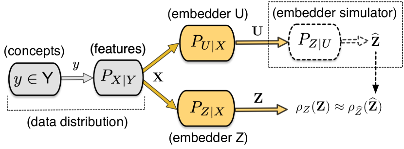
Figure 1: Communicating a concept $y\in\mathsf{Y}$ over two embedding models with prediction $\rho_{Z}(Z)$.

From an information-theoretic perspective [27], the quality of an embedding model can be likened to the capacity of a noisy communication channel with an uncoded input (e.g., a text, a molecule…), where a downstream task of interest is performed at the output (the embedding) of the channel. Let $Y\in\mathsf{Y}$ represent the message (the source) to be communicated over both channels; $X$ represents the transmitted signal; and $P_{U|X}$ and $P_{Z|X}$ the communication channels with outputs $U$ and $Z$, respectively. This process is illustrated in Figure 1. It naturally satisfies the Markov chain $Y\leftrightarrow X\leftrightarrow(U,Z)$. A desirable property is that the embedding models $U$ and $Z$ retain as much pertinent information as feasible to predict $Y$.

We shall be interested in the underlying information relationships between those embedding models that can be interpreted as channel $U$ being "more informative" for communicating $Y$ than channel $Z$. The first attempt to introduce an ordering between communication channels appears in Shannon [94]. Körner and Marton later introduced [57] the concepts of "less noisy" (or more informative) and "degraded" (or sufficiency) orderings between channels.

Definition 1 (Sufficiency and informativeness orderings [57]).

Let $P_{U|X}$ and $P_{Z|X}$ be two Markov kernels (embedding models).

• Sufficiency $U\succcurlyeq_{S}Z$. The embedding model $P_{U|X}$ is said to be "sufficient" for the embedding model $P_{U|X}$ (or $Z$ to be degraded w.r.t. $U$) if and only if there exists another Markov kernel $M\in\mathcal{T}(\mathsf{Z}|\mathsf{U})$ such that $\|M\!\circ\!P_{U|X}-P_{Z|X}\|_{\text{TV}}=0$, i.e. $Z$ can be simulated from $U$ using $M$ without information loss).

• More informative $U\succcurlyeq_{I}Z$. The embedding model $P_{U|X}$ is said to be "more informative" (or less noisy) than $P_{Z|X}$ if and only if the embedding models always satisfy the inequality

  $$I(Y;U)\geqslant I(Y;Z),\quad\forall P_{YX}\in\mathcal{P}(\mathsf{Y}\times\mathsf{X}).$$

Proposition 1 (Relationships of sufficiency and information).

The following relationships hold:

• Sufficiency $\Rightarrow$ informativeness. If the embedding model $P_{U|X}$ is sufficient for the embedding model $P_{Z|X}$, i.e. $U\succcurlyeq_{S}Z$, then $U\succcurlyeq_{I}Z$. However, Informativeness $\nRightarrow$ sufficiency.

• Informativeness $\Rightarrow$ higher capacity to distinguish concepts. If the embedding model $P_{U|X}$ is more informative than embedding model $P_{Z|X}$, i.e. $U\succcurlyeq_{I}Z$, then

  $$\textrm{KL}\big{(}P_{U|Y}(\cdot|y_{0})\|P_{U|Y}(\cdot|y_{1})\big{)}\geqslant\textrm{KL}\big{(}P_{Z|Y}(\cdot|y_{0})\|P_{Z|Y}(\cdot|y_{1})\big{)},$$

  for any pair of concepts $(y_{0},y_{1})\in\mathsf{Y}\times\mathsf{Y}$ and all probability distributions $P_{YX}$.

Remark 1.

An immediate consequence of claim (i) is that the sufficient condition between embedding models implies that the embedding model $U$ is more informative than the embedding model $Z$ relative to all target concepts in $\mathsf{Y}$ over all possible data distributions: $I(Y;U)\geqslant I(Y;Z)$, for all probability distributions $P_{YX}$.

Although $U$ being more informative than $Z$ does not necessarily imply $U\succcurlyeq_{S}Z$ [57, 66]; (ii) states that being more informative ensures a higher statistical discrimination capacity between any pairs of target concepts (for further discussion, see Sec. B.2).

Motivated by the concepts of sufficiency and informativeness between embedding models, we can inquire about their statistical consequences for a learner conducting an inference task on these embeddings. More precisely, given a finite set of concepts $\mathsf{Y}$, if $U\succcurlyeq_{S}Z$, is the Bayes risk expected to be smaller when the inference is based on $U$ than when it is based on $Z$?

2.3 Comparing statistical experiments with embedding Models

The pursuit of comparing statistical experiments originated from the seminal paper by Bohnenblust, Shapley, and Sherman [16], followed by subsequent contributions by Blackwell [13, 14]. They formally established the relationships between sufficiency (Def. 1) and inference procedures.

In our framework, a statistical experiment [13] consists of a mathematical abstraction (see Appendix A for further details) intended to represent a downstream task where a learner aims at inferring a concept $y\in\mathsf{Y}$ from the embeddings $U$ or $Z$. Deciding what embedder should be used to perform a given task is too general. In this work, we do not take into account the computational cost or the size of an embedder and solely focus on the following question:

What are the necessary and sufficient conditions that ensure that employing the embedding $U$ for any task $P_{YX}$ leads to lower risk compared to using the embedding $Z$?

Drawing parallels with the theoretical framework established for comparing statistical experiments, a relationship can be derived between the concept of sufficiency and the expected risk for a specific task (see Sec. B.5 for further discussion).

We concentrate on the scenario where $\mathsf{Y}$ consists of a finite number of concepts (e.g., classification tasks), as it is a significant case in its own right [104] and provide fundamental insights for the present work. The next Proposition states an important relation between the concept of sufficiency and the expected Bayes risk on any classification task.

Proposition 2 (Comparison of embedding models through Bayes risks).

Given two embedding models $P_{U|X}\in\mathcal{K}(\mathsf{U}|\mathsf{X})$ and $P_{Z|X}\in\mathcal{K}(\mathsf{Z}|\mathsf{X})$, the following statements are equivalent:

1. The embedding model $P_{U|X}$ is sufficient relative to $P_{Z|X}$, i.e. $U\succcurlyeq_{S}Z$.

2. For all probability measures $P_{YX}$ on finite alphabets $\mathsf{Y}\times\mathsf{X}$, the expected Bayes risks satisfy

   $$\inf_{\rho_{U}:\mathsf{U}\rightarrow\mathcal{P}(\mathsf{Y})}\Pr\big{(}\rho_{Y}(U)\neq Y\big{)}\leqslant\inf_{\rho_{Z}:\mathsf{Z}\rightarrow\mathcal{P}(\mathsf{Y})}\Pr\big{(}\rho_{Z}(Z)\neq Y\big{)}.$$

Remark 2.

In other words, if we can fully simulate an embedder $Z$ from another embedder $U$, the expected risk across all potential classification tasks cannot be greater when using $U$ compared to $Z$. The proof of this Proposition is given in Sec. B.3. It is worth mentioning that various versions of this result are available in the literature [104]. However, our extension here, in a simpler setting, incorporates concepts and features into the experiment comparison framework.

2.4 Challenges in ranking embedding models and their deficiency

According to the notion of "sufficiency", we can distinguish the three following possibilities:

• Equivalence: $U\succcurlyeq_{S}Z$ and $Z\succcurlyeq_{S}U$ denoted $U\approx Z$. U and Z can simulate each other.

• Comparability: $U\succcurlyeq_{S}Z$ but $Z\not\succcurlyeq_{S}U$ only Z can be simulated from U.

• Non-comparability: $U\not\succcurlyeq_{S}Z$ and $Z\not\succcurlyeq_{S}U$, neither U nor Z can simulate each other.

Our results up to now only account for the two first possibilities. However, two embedders are generally not comparable (Sec. B.4). This issue was addressed by Le Cam [63], who introduced the notion of "deficiency".

Definition 2.

The deficiency $\delta(P_{U|X}\rightarrow P_{Z|X})$ of $P_{Z|X}$ relative to $P_{U|X}$ is defined as [63]

$$\delta(P_{U|X}\rightarrow P_{Z|X})\triangleq\inf_{M\in\mathcal{K}(\mathsf{Z}|\mathsf{U})}\|M\!\circ\!P_{U|X}-P_{Z|X}\|_{\text{TV}},$$

where the infimum is taken over all Markov kernels (or transition probabilities) $M\in\mathcal{K}(\mathsf{Z}|\mathsf{U})$, mapping stochastically $\mathsf{U}$ and $\mathsf{Z}$, and $\delta$ measures error between the simulated and true embedders.

$\delta$ indicates how well one model can be reconstructed from the other, it induces a natural relaxation of the sufficiency where the reconstruction does not have to be perfect for us to obtain guarantees on the downstream tasks performance (See Corollary 1). It avoids the non-comparability problem by evaluating "how much information" we lose when passing from one model to the other one.

Le Cam [63] showed that, for a given task $Y$, the deficiency $\delta(P_{U|Y}\rightarrow P_{Z|Y})$ is directly related to the expected Bayes risks on the task (see Sec. B.6). We extend this result to the comparison of two embedding models $P_{U|X}$ and $P_{Z|X}$ in a task-agnostic manner and build the relation to the expected Bayes risks for any classification task $Y$, defined as $\mathcal{R}_{U}(Y)\triangleq\inf\limits_{\rho_{U}:\mathsf{U}\rightarrow\mathcal{P}(\mathsf{Y})}\Pr\big{(}\rho_{U}(U)\neq Y\big{)}$.

Corollary 1.

Given two embedding models $P_{U|X}$ and $P_{Z|X}$, the following statements are equivalent:

1. The deficiency $\delta(P_{U|X}\rightarrow P_{Z|X})\leqslant\epsilon$.

2. For any probability distribution $P_{YX}$ on finite alphabets $\mathsf{Y}\times\mathsf{X}$, there exists $\epsilon>0$ satisfying

   $$\mathcal{R}_{U}(Y)-\epsilon|\mathsf{X}|\leqslant\mathcal{R}_{Z}(Y).$$

The proof of this Corollary is relegated to Sec. B.3.

Remark 3.

In particular, we can infer that for any classification task $Y$, the expected Bayes risk of the embedding model $U$ is upper bounded by the expected Bayes risk of the embedding model $Z$:

$$\mathcal{R}_{U}(Y)-\mathcal{R}_{Z}(Y)\leqslant|\mathsf{X}|\delta(P_{U|X}\rightarrow P_{Z|X}),\quad\textrm{for all distributions $P_{YX}$, }$$

and similarly, $|\mathcal{R}_{U}(Y)-\mathcal{R}_{Z}(Y)|\leqslant|\mathsf{X}|\max\big{\{}\delta(P_{U|X}\rightarrow P_{Z|X}),\delta(P_{Z|X}\rightarrow P_{U|X})\big{\}}$, for all distributions $P_{YX}$. If both deficiencies are small, the resulting expected Bayes risks of the embedding models $U$ and $Z$ will be close to each other for any target task $Y$.

3 Quantifying Information Sufficiency Between Embedding Models

We want to compare embedding models using the concept of deficiency, leveraging Prop. 2 and Corollary 1. These propositions suggest that the performance on any classification task of an embedding model $U$ relative to the model $Z$ is bounded by $\delta(P_{U|X}\rightarrow P_{Z|X})$. However, estimating the deficiency from data samples is notably challenging [95], and while upper bounds derivation exists, they do not necessarily make it tractable.

3.1 Estimating Information Sufficiency

The deficiency $\delta(P_{U|X}\rightarrow P_{Z|X})$ between two embedding models $P_{U|X}$ and $P_{Z|X}$, measures how well $U$ can be used to simulate $Z$ using a Markov kernel $M\in\mathcal{K}(\mathsf{Z}|\mathsf{U})$. This section aims to build a tractable proxy for this reconstruction cost. To this end, we estimate how much we can reduce the uncertainty about $Z$ by observing $U$ by learning an appropriate Markov kernel. This corresponds to the information sufficiency [29, 4] and can be interpreted as the information-theoretic counterpart of the deficiency. The information deficiency between $U$ and $Z$ is then defined as:

Definition 3 (Information sufficiency).

The information sufficiency $\mathcal{I}_{S}(U\rightarrow Z)$, relative to parametric classes of distributions $\mathcal{F}_{\Theta}(\mathsf{Z})$ and $\mathcal{K}_{\Theta}(\mathsf{Z}|\mathsf{U})$ (multivariate Gaussian mixtures [82]) is defined:

$$\mathcal{I}_{S}(U\rightarrow Z)\triangleq\underbrace{\inf_{f\in\mathcal{F}_{\Theta}(\mathsf{Z})}\mathbb{E}\left[-\log f(Z)\right]}_{\text{Uncertainty of }Z}-\underbrace{\mathbb{E}\left[\inf_{M\in\mathcal{K}_{\Theta}(\mathsf{Z}|\mathsf{U})}\mathbb{E}\left[-\log M(Z|U)|U\right]\right]}_{\text{Uncertainty when simulating }Z\text{ from }U\text{ with }M}.$$ (1)

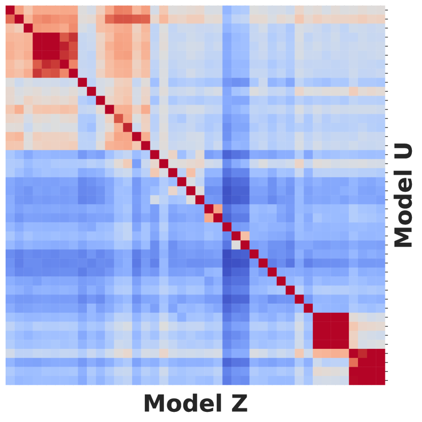
Figure 2: Pairwise $\mathcal{I}_{S}$ for text embedders.

Remark 4.

When the information sufficiency $\mathcal{I}_{S}(U\rightarrow Z)$ is large, it signifies that $U$ offers a substantial amount of information to simulate $Z$, a proxy for a small deficiency. Conversely, when $\mathcal{I}_{S}(U\rightarrow Z)$ is lower, it implies that the channel $P_{Z|Y}$ is subject to considerable noise or randomness, leading to a greater loss of statistical information.

We hence attempt to simulate $Z$ from $U$ by learning a Markov kernel $M\in\mathcal{K}_{\Theta}(\mathsf{Z}|\mathsf{U})$, via a mixture of multivariate Gaussians, and measure the uncertainty reduction it induces.

Pairwise embedder evaluation.

For set of embbeders $(Z_{k})_{k}$ represented by their Markov kernels $\{P_{Z_{k}|X}\}_{k}$, we compute the pairwise information sufficiency $\mathcal{I}_{S}(Z_{k}\rightarrow Z_{l})$. The pairwise information sufficiency matrix defines the adjacency matrix of a directed graph of embedders (Figure 2). Corollary 1 shows that embedders sharing high information sufficiency are expected to perform similarly on any downstream tasks, motivating the identification of communities in the graph. While the graph construction is in $\mathcal{O}(N^{2})$; where $N$ is the number of embedders, it is in practice tractable for a reasonable number of embedders (the reader is referred to Sec. E.5) for more details).

Practical embedding evaluation.

We construct the set of all information sufficiency using $Z_{k}$: $\mathcal{S}_{\mathcal{I_{S}}}\left(k\right)=\left\{\mathcal{I}_{S}(Z_{k}\rightarrow Z_{l})\right\}_{l\not=k}$. We build our information sufficiency score ($\overline{\mathcal{I}_{S}}$ score) by taking the median of $\mathcal{S}_{\mathcal{I_{S}}}\left(k\right)$. Details on the $\overline{\mathcal{I}_{S}}$ score’s estimation, such as the motivation behind the median choice, can be found in Sec. E.1.

4 Experimental Setup

We aim to evaluate the practical utility of the $\overline{\mathcal{I}_{S}}$ score to rank and select the best embedders for a given data distribution. We compare this ranking to those obtained on various downstream tasks. Our experimental protocol is divided into three main steps:

1. We evaluate the $\overline{\mathcal{I}_{S}}$ score of the models by identifying a large and diverse dataset that is supposed to be representative of the data distribution of interest.

2. We train a small feedforward neural network ($\rho_{Z_{k}}$) per embedder $P_{Z_{k}|X}$ to perform each downstream task and record its performances ($R^{2}$ score for regression, AUROC/accuracy for binary/multiclass classification).

3. We compare the models’ performances on the downstream tasks and the $\overline{\mathcal{I}_{S}}$ score by measuring three types of correlations: the Pearson correlation, the Spearman correlation, and the Kendall-Tau coefficient.

	$\varrho_{p}$	$\varrho_{s}$	$\tau$
Retrieval (15 datasets)	0.89	0.89	0.69
Classification (12 datasets)	0.92	0.88	0.73
Clustering (11 datasets)	0.86	0.85	0.66
STS (10 datasets)	0.92	0.83	0.63
Reranking (4 datasets)	0.84	0.78	0.64
Average (56 datasets)	0.94	0.90	0.73
Additional Classif (8 datasets)	0.89	0.84	0.66

(a) NLP

	$\varrho_{p}$	$\varrho_{s}$	$\tau$
Absorption (8 datasets)	-	0.89	0.70
Distribution (3 datasets)	-	0.89	0.70
Metabolism (8 datasets)	-	0.94	0.79
Excretion (3 datasets)	-	0.77	0.60
Toxicity (9 datasets)	-	0.92	0.75
ADMET (31 datasets)	-	0.94	0.80
DTI (1496 tasks) see Sec. D.4	-	0.88	0.70

(b) Molecular Modelling

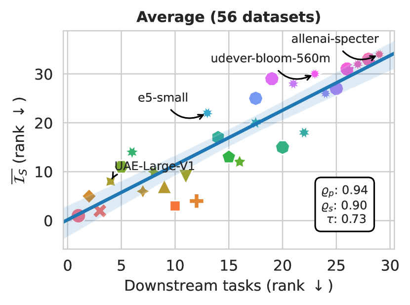
(a) NLP

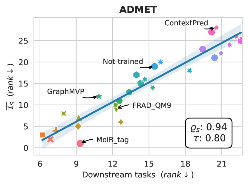
(b) Molecular Modelling

Figure 3: Correlation between $\overline{\mathcal{I}_{S}}$ scores and downstream task performances in (a) NLP and (b) Molecular Modelling. $\varrho_{p}$ is the Pearson correlation, $\varrho_{s}$ is the spearman correlation, and $\tau$ is the Kendall-Tau coefficient. See Sec. C.3.1 for unaggregated results in NLP and Sec. D.3 in molecular modeling.

5 Text Embeddings Evaluation

5.1 Experimental setting

Embedders & Datasets.

We compared $34$ models with different training objectives, training datasets, and architectures. We included embedders derived from modern LLM such as LLaMA [106], Mistral [52], Gemma [102], Croissant [37] and T5 encoders [77]; common embedders derived from BERT architectures [31, 38, 85] or RobERTa [41] and embedders trained on specific embeddings objectives such Angle [64], Stella, E5 models [113], LaBSE [38]. A comprehensive list of the models can be found in Sec. C.1, Tab. 1 with their main characteristics and links to the Huggingface Hub for reproducibility. We used them to extract embeddings for many different datasets from the MTEB benchmark such as Banking77 [19], Sickr [122], Amazon polarity [72], SNLI [120] and IMDB [70]. We provide the datasets statistics in Sec. C.1, Tab. 2.

Downstream tasks evaluation.

We rely on the results released on the MTEB leaderboard and compare our rankings to the rankings and scores obtained by the different models on the different tasks. We evaluate additional tasks that are not included in the MTEB benchmark, such as tweet_eval [8, 74, 7, 109, 9], DAIR Emotion [92], agnews topic classification [123], Clinc intent detection [62] PAWS-X [118] and Rotten Tomatoes [79].

5.2 Model’s Information Sufficiency analysis

(a)

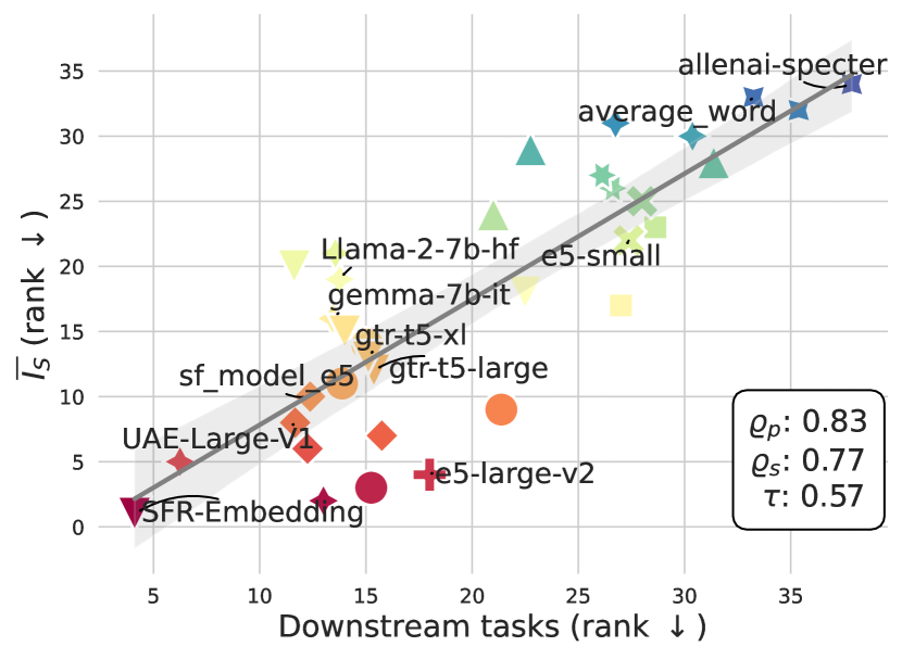
(b)

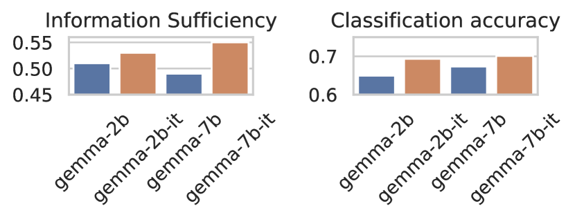
(c)

Figure 4: 4(a), presents the information sufficiency directed graph and the induced communities. 4(b) displays the performance on additional downstream tasks and models not evaluated in the MTEB leaderboard. 4(c) shows that instruction finetuning positively impacts the models’ performance on the downstream tasks and that this improvement is captured by $\overline{\mathcal{I}_{S}}$.

Correlation with downstream tasks performance.

The MTEB Benchmark offers a natural starting point to compare models’ ranking according to their performance on downstream tasks and their $\overline{\mathcal{I}_{S}}$ score. In 3(a), we show that the $\overline{\mathcal{I}_{S}}$ score of an embedder correlates positively with its performance on a wide range of downstream tasks, from classification and similarity tasks to retrieval and clustering tasks. Overall, our $\overline{\mathcal{I}_{S}}$ score correlates strongly with MTEB’s average score (Spearman correlation of $0.90$ and a Pearson correlation of $0.94$, see 3(a)) and with the subtask performance 1(a)). We extended our experiments to a more extensive set of models not included in the MTEB benchmark and observed a similar trend (4(b)). Per-datasets results are reported in Sec. C.3.1 and ablations in Sec. C.3.2. All our results show that our estimation of the information sufficiency between models is a good proxy for the performance of the models on a wide range of tasks.

Embedder communities.

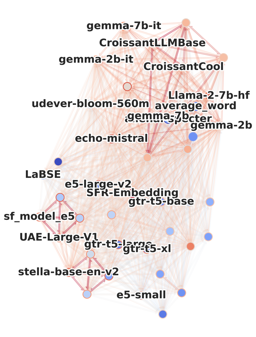
(a)

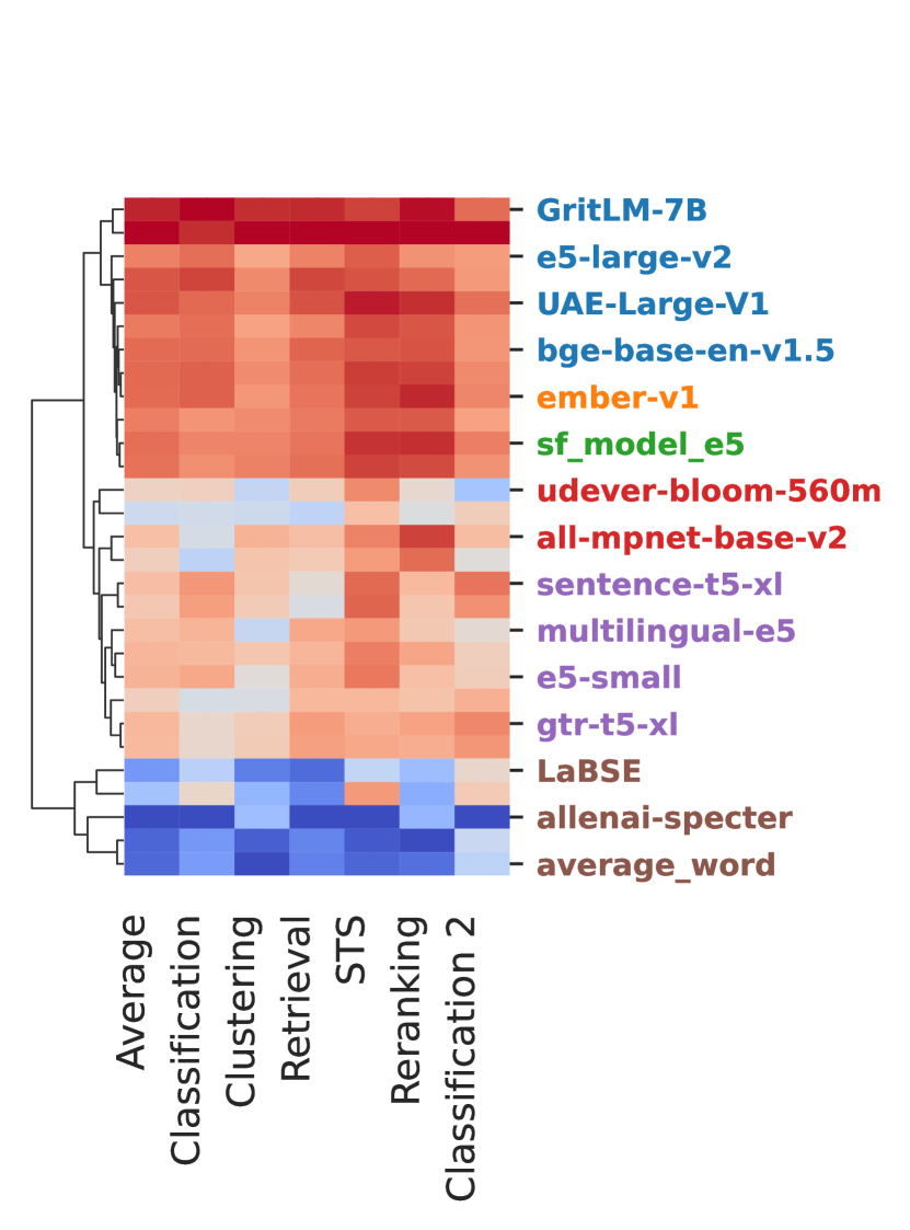
(b)

Figure 8: We present different interesting properties of $\overline{\mathcal{I}_{S}}$. In 4(a), we show that it can be used to cluster models 8(b), reports the performance of the models on the different task categories. They are grouped by similar behaviors on these tasks (dendrograms) and colored by the communities discovered in the information sufficiency graph. (Only models evaluated as part of the MTEB benchmark are shown).

The pair-wise information sufficiency evaluation between the models can be used to cluster them into communities [15](4(a), Figure 2). We observe that the extracted clusters group together models that are similar in their training objectives and architectures. LLM-based models such as LLaMA, Mistral, Gemma, and Croissant are clustered together, while BERT-based models share another cluster. Similarly, models trained specifically for embedding purposes, such as UAE-Large-V1 and ember-v1, are grouped together. This suggests that the ordering induced by information sufficiency is meaningful and can be used to identify models with similar properties and behaviors. Consistently with Corollary 1, we observe that the performance of the models on the downstream tasks is similar within the same cluster (Figure 8). In addition, we found that it captures improvements by both steps of pretraining and instruction fine-tuning (4(c), Sec. C.3.2)

6 Molecular Modeling

6.1 Experimental setting

Embedders. To process molecular data, embedders can leverage different representations of the molecules, providing an interesting benchmark to evaluate the $\overline{\mathcal{I}_{S}}$ score. We evaluated models derived from the molecular representation learning literature, summed up in  Sec. D.1. We considered various input modalities such as string representations (SMILES [114], SELFIES [58]), 2D-graphs by using graph neural networks (GNNs), and 3D-representations (using the TorchMD-net architecture [80]). We added a randomly initialized baseline GNN model that was not trained on any dataset.

Datasets. To evaluate the information sufficiency between embedders, we compared the models on the ZINC 250k dataset[50], designed to gather compounds that could be relevant to a wide range of therapeutic projects. This dataset contains 250k commercially available compounds meant to be used in diverse therapeutic projects.

Downstream tasks. We evaluated the embedders on 31 downstream tasks extracted from the Therapeutic Data Commons [49] platform. This section focuses on ADMET tasks (Absorption, Distribution, Metabolism, Excretion, and Toxicity). Results on Drug-Target interaction tasks can be found in Sec. D.4. Datasets collected are split into a training, validation, and test set, following the scaffold-split strategy, further described in see Sec. D.3.

6.2 Model’s Information Sufficiency analysis

(a)

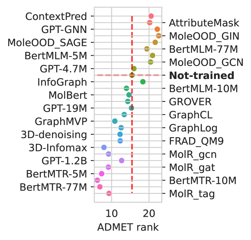
(b)

Figure 5: (a) Pairwise information sufficiency graph between the embedders. The center color represents the ability to simulate other models, while the surrounding colors represent the ability to be simulated by other models. Red indicates a high ability to simulate or be simulated, while blue indicates a low ability. (b) Mean rank of the models (ordered by $\overline{\mathcal{I}_{S}}$ score) on downstream tasks.

Global results. The $\overline{\mathcal{I}_{S}}$ score ranking is consistent with the results of the embedders on the ADMET downstream tasks, achieving a Spearman correlation of 0.95 and a Kendall-tau coefficient of 0.80, as reported in 3(b). Detailed results for each of the 31 tasks are available in Sec. D.3 in Tab. 6. Table 1(b) shows the correlation between the $\overline{\mathcal{I}_{S}}$ score rankings and the performances obtained on the ADMET tasks within each category. High correlations are achieved within most task categories, especially when large tasks are available (containing an important number of molecules). On excretion tasks, the correlation is lower (below $0.8$), which can be explained by the fact that these tasks are the most challenging regression tasks available, where the fine-tuned models reach the lowest $R^{2}$ scores between $0$ and $0.2$ (see Sec. D.3).

Most / Least promising models. We observe in 5(b) that the most promising models are the (Chem)Bert-MTR models[3] and MolR[112], the former trained on SMILES representations to predict a variety of computationally available molecular properties, and the latter trained on 2D graphs to preserve equivalence of molecules w.r.t chemical reactions. Surprisingly, these models share high predictive mutual information (being assigned to the same Louvain community in 5(a)), suggesting that they capture similar information despite significant differences in their training methods. These models also appear to be the most competitive on the ADMET tasks. On the other hand, and consistently with Sun et al. [99]’s observation, training methods for 2D-GNNs such as following attribute masking and context prediction objective are deemed as the least informative according to the $\overline{\mathcal{I}_{S}}$ score. This is explained by the simplicity of these pretraining objectives for this data modality. These methods are also among the least competitive methods on the ADMET downstream tasks.

NLP-inspired models. (Chem)Bert-MLM [3], MolBert [36] and (Chem)GPT[40] leverage masked language model objective applied to string representations (SMILES and SELFIES). Unsurprisingly, as seen in 5(a), these models are clustered, suggesting they capture similar information. However, they fail to simulate other models in the pool, resulting in low $\overline{\mathcal{I}_{S}}$ scores, a result consistent with the known limitations of these pretraining objectives [23, 105]. A noticeable exception is (Chem)GPT-1.2B (the biggest model of the pool by far), which displays a significantly higher $\overline{\mathcal{I}_{S}}$ score.

"Not-trained" GNN. 5(b) helps visualize the performances of the different models relative to our baseline "Not-trained" GNN. Surprisingly, some models are ranked less promising than this baseline by the $\overline{\mathcal{I}_{S}}$ score. However, all of these less promising models obtain poorer performances on the downstream tasks. Similarly, except for InfoGraph [98], every model ranked more promising than the "Not-trained" GNN baseline and obtained better results on ADMET tasks. This surprising result validates evaluation of the $\overline{\mathcal{I}_{S}}$ score w.r.t this baseline.

7 Limitations and Conclusions

We proposed a principled approach to embedding model evaluation by framing model ranking as a variation of comparing statistical experiments. Utilizing concepts of sufficiency, informativeness, and deficiency, we developed mathematically grounded metrics for pairwise comparisons between embedders without relying on labeled data in downstream tasks. Our tractable relaxation, termed information sufficiency, demonstrated strong correlations with rankings based on downstream task performance in extensive experiments. Although successful, our method still has at least two primary limitations. First, its effectiveness depends on the number and diversity of available embedders (see Sec. E.4). Future work could explore using randomly initialized embedders (random projections) instead of pre-trained ones. Second, we can enhance our proxy for predicting the deficiency between models by exploring better methods (e.g., estimating the $f$-divergence) to directly learn the Markov kernel that minimizes the total variation distance, which we leave for future research.

Appendix

Appendix A Background and Notation

We consider all alphabets to be standard Borel [28] (i.e., isomorphic to a Borel subspace of a Polish space), encompassing virtually all practical scenarios. Each such space $\mathsf{Y}$ is equipped with its Borel $\sigma$-algebra $\mathcal{B}(\mathsf{Y})$. The set of all probability measures on $\mathsf{Y}$ is denoted by $\mathcal{P}(\mathsf{Y})$. The total variation distance between $P$ and $Q$ in $\mathcal{P}(\mathsf{Y})$ is defined as

$$\|P-Q\|_{\textrm{TV}}=\sup_{\mathcal{A}\in\mathcal{B}(\mathsf{Y})}|P(\mathcal{A})-Q(\mathcal{A})|,$$ (2)

and the Kullback–Leibler divergence is defined by

$$\textrm{KL}\big{(}P\|Q\big{)}=\left\{\displaystyle\begin{array}[]{cc}\displaystyle\int_{\mathsf{X}}\log\frac{\mathsf{d}P}{\mathsf{d}Q}\mathsf{d}P&\textrm{if }\,P\ll Q\\ +\infty&\textrm{otherwise.}\end{array}\right.$$ (3)

Given a joint probability measure $P_{XY}$ in $\mathcal{P}(\mathsf{X}\times\mathsf{Y})$ induced by two random variables $X\in\mathsf{X}$ and $Y\in\mathsf{Y}$ with product measures $P_{X}P_{Y}$, the Mutual Information is defined as $I(X;Y)=\textrm{KL}\big{(}P_{XY}\|P_{X}P_{Y}\big{)}$. If $P_{X}\in\mathcal{P}(\mathsf{X})$ is a probability measure induced by $X\in\mathsf{X}$, the Differential Entropy is defined by

$$h(X)=-\int_{\mathsf{X}}\log\frac{\mathsf{d}P_{X}}{\mathsf{d}\mu}\,dP_{X},$$ (4)

where $\mu$ denotes the Lebesgue measure. Similarly, it is possible to define the conditional entropy of $Y$ given $X$ which is denoted by $h(Y|X)$. The mutual information satisfies the identities $I(X;Y)=h(Y)-h(Y|X)=h(X)-h(X|Y)$ and $h(Y|X)\leqslant h(Y)$ (see [27] for further details).

A Markov (or transition probability) kernel between $\mathsf{X}$ and $\mathsf{Y}$ is a mapping $T:\mathcal{B}(\mathsf{Y})\times\mathsf{X}\to[0,1]$, satisfying $T(\cdot|x)\in\mathcal{P}(\mathsf{Y})$ for all $x\in\mathsf{X}$ and $T(\mathcal{B}|\cdot)$ being a measurable function on $\mathsf{X}$ for any $B\in\mathcal{B}(\mathsf{Y})$. The space of all such $T$ is denoted by $\mathcal{K}(\mathsf{Y}|\mathsf{X})$. In cases where both $\mathsf{Y}$ and $\mathsf{X}$ are finite, any $\mathcal{K}(\mathsf{Y}|\mathsf{X})$ is represented as a stochastic matrix with elements $T(y|x)$, $(x,y)\in\mathsf{X}\times\mathsf{Y}$. Every $T\in\mathcal{K}(\mathsf{Y}|\mathsf{X})$ induces a mapping $\mathcal{P}(\mathsf{X})\longrightarrow\mathcal{P}(\mathsf{Y})$, denoted by $T$, mapping any $P\in\mathcal{P}(\mathsf{X})$ to $Q=T\!\circ\!P\in\mathcal{P}(\mathsf{Y})$, where

$$Q(B)=(T\!\circ\!P)(B)\triangleq\int_{\mathsf{X}}T(B|x)P(\mathsf{d}x),\quad\forall B\in\mathcal{B}(\mathsf{Y}).$$ (5)

We denote the composition of Markov kernels by juxtaposition: for $M\in\mathcal{K}(\mathsf{Z}|\mathsf{Y})$ and $T\in\mathcal{K}(\mathsf{Y}|\mathsf{X})$, their composition $M\!\circ\!T\in\mathcal{T}(\mathsf{Z}|\mathsf{X})$ is defined by

$$(M\!\circ\!T)(Z|x)\triangleq\int_{\mathsf{Y}}M(Z|y)T(\mathsf{d}y|x),\quad\forall x\in\mathsf{X},\,Z\in\mathcal{B}(\mathsf{Z}).$$ (6)

We define the total variation distance between two Markov kernels $T,T^{\prime}\in\mathcal{K}(\mathsf{Y}|\mathsf{X})$ as follows:

$$\|T-T^{\prime}\|_{\textrm{TV}}\triangleq\sup_{x\in\mathsf{X}}\|T(\cdot|x)-T^{\prime}(\cdot|x)\|_{\textrm{TV}}.$$ (7)

A statistical model is a triple $\mathcal{M}_{U}\equiv\big{(}\mathsf{U},\mathcal{B}(\mathsf{U}),(P_{U|Y}(\cdot|y):y\in\mathsf{Y})\big{)}$, where $(\mathsf{U},\mathcal{B}(\mathsf{U}))$ is a sample space; $\mathsf{Y}$ is a concept space, and $P_{U|Y}:\mathcal{B}(\mathsf{U})\times\mathsf{Y}\to[0,1]$ is a Markov kernel (or transition probability).

Appendix B Proofs Theoretical Results

Proposition 3 (Relationships of sufficiency and information).

The following relationships hold:

• Sufficiency $\Rightarrow$ informativeness. If the embedding model $P_{U|X}$ is sufficient for the embedding model $P_{Z|X}$, i.e. $U\succcurlyeq_{S}Z$, then $U\succcurlyeq_{I}Z$. However, Informativeness $\nRightarrow$ sufficiency.

• Informativeness $\Rightarrow$ higher capacity to distinguish concepts. If the embedding model $P_{U|X}$ is more informative than embedding model $P_{Z|X}$, i.e. $U\succcurlyeq_{I}Z$, then

  $$\textrm{KL}\big{(}P_{U|Y}(\cdot|y_{0})\|P_{U|Y}(\cdot|y_{1})\big{)}\geqslant\textrm{KL}\big{(}P_{Z|Y}(\cdot|y_{0})\|P_{Z|Y}(\cdot|y_{1})\big{)},$$

  for any pair of concepts $(y_{0},y_{1})\in\mathsf{Y}\times\mathsf{Y}$ and all probability distributions $P_{YX}$.

B.1 Proof Proposition 1

Proof.

It is immediate to check that the data-processing inequality and the Markov chain $Y\leftrightarrow X\leftrightarrow U\leftrightarrow Z$ implies the relation in claim (i). On the other hand, (ii) is proved by means of an explicit counterexample [57]. Given any $0<p<1/2$ with $\bar{p}=1-p$. For some $\epsilon,\delta>0$, consider two discrete embedding models defined by the following matrices:

$$P_{Z|X}=P_{U|X}\left(\begin{array}[]{cc}1+\epsilon&1-\epsilon\\ 1/2&1/2\end{array}\right)\quad\textrm{with}\quad P_{U|X}=\left(\begin{array}[]{cc}p&\bar{p}\\ p+\delta&\bar{p}-\delta\end{array}\right).$$ (8)

By taking $\epsilon,\delta>0$ small enough, both $P_{U|X}$ and $P_{Z|X}$ are stochastic matrices. It follows that $P_{Z|X}$ is not a degraded version of $P_{U|X}$ but provided that $\epsilon,\delta$ are sufficient small, the embedding model $P_{U|X}$ is more informative than $P_{Z|X}$, which proves the claim.

In order to show (iii), let $P_{U|Y}$ and $P_{Z|Y}$ be the corresponding probability measures induced by $P_{X|U}(\cdot|u)$ via the embedding models:

$$P_{U|Y}(U|y)=\int_{\mathsf{X}}P_{U|X}(U|x)P_{X|Y}(\mathsf{d}x|y),\quad\forall y\in\mathsf{Y},\,U\in\mathcal{B}(\mathsf{U}),$$ (9)

and

$$P_{Z|Y}(Z|y)=\int_{\mathsf{X}}P_{Z|X}(Z|x)P_{X|Y}(\mathsf{d}x|y),\quad\forall y\in\mathsf{Y},\,Z\in\mathcal{B}(\mathsf{Z}),$$ (10)

for any $y\in\mathsf{Y}=\{y_{0},y_{1}\}$. For a $0\leqslant\lambda\leqslant 1$, let $P_{X|Y}(\cdot|y_{0})\in\mathcal{P}(\mathsf{X})$ and $P_{X|Y}(\cdot|y_{1})\in\mathcal{P}(\mathsf{X})$ be two arbitrary probability measures on $\mathsf{X}$. Let $P_{X|Y}(X|y)$ be defined by

$$P_{X|Y}(X|y)=\mathbbm{1}[y=y_{0}]P_{X|Y}(X|y_{0})+\mathbbm{1}[y=y_{1}]P_{X|Y}(X|y_{1}).$$

By replacing it into equations (9) and (10), we obtain

$$P_{U|Y}(U|y)=\mathbbm{1}[y=y_{0}]P_{U|Y}(U|y_{0})+\mathbbm{1}[y=y_{1}]P_{U|Y}(U|y_{1})$$ (11)

$$P_{Z|Y}(Z|y)=\mathbbm{1}[y=y_{0}]P_{Z|Y}(Z|y_{0})+\mathbbm{1}[y=y_{1}]P_{Z|Y}(Z|y_{1})$$ (12)

and let $P_{Y}(y_{0})=\lambda$ and $P_{Y}(y_{1})=1-\lambda$. The above probability measures correspond to a quadruple of random variables: $(Y_{\lambda},X_{\lambda},U_{\lambda},Z_{\lambda})\in\mathcal{P}(\mathsf{Y}\times\mathsf{X}\times\mathsf{U}\times\mathsf{Z})$. Consider the function $f(\lambda)$ defined by

$$f(\lambda)=I(Y_{\lambda};U_{\lambda})-I(Y_{\lambda};Z_{\lambda}).$$

It is not difficult to check that $f(\lambda)\geqslant 0$ for all $0\leqslant\lambda\leqslant 1$, and $f(0)=0$ which requires that $f^{\prime}(0)\geqslant 0$. By taking the differentiation, we obtain

$$f^{\prime}(0)=\textrm{KL}\big{(}P_{U|Y}(\cdot|y_{0})\|P_{U|Y}(\cdot|y_{1})\big{)}-\textrm{KL}\big{(}P_{Z|Y}(\cdot|y_{0})\|P_{Z|Y}(\cdot|y_{1})\big{)}\geqslant 0,$$

which implies the claim (iii). This concludes the proof. ∎

B.2 Comments about capacity to distinguish concepts

Notice that the KL divergence between the induced distributions of the resulting embedding is not less for the embedding model $U$ than $Z$. Indeed, consider the case of binary classification $\mathsf{Y}=\{y_{0},y_{1}\}$ with uniformly distributed concepts. Pinsker’s inequality [108] together with claim (iii) imply

$$\textrm{KL}\big{(}P_{U|Y}(\cdot|y_{0})\|P_{U|Y}(\cdot|y_{1})\big{)}\geqslant 2\|P_{Z|Y}(\cdot|y_{0})-P_{Z|Y}(\cdot|y_{1})\|_{\textrm{TV}}^{2}.$$

From which, it is easy to verify that the accuracy of the expected Bayes accuracy of the optimal classifier based on $Z$ is upper bounded by [108, Lemma 2.1]:

$$\sup_{\psi}\Pr(\psi(Z)=Y)\leqslant 1-\frac{1}{2}\exp\left(-\textrm{KL}\big{(}P_{U|Y}(\cdot|y_{0})\|P_{U|Y}(\cdot|y_{1})\big{)}\right),$$

where the exponent in the upper bound is subject to the discriminating capacity through the KL divergence of the embedding model $U$ on $\mathsf{U}$.

B.3 Proof of Proposition 2 and Corollary 1

We begin with the proof of Proposition 2.

Proof.

Clearly, the assumption (i) implies the statement (ii) by Data-Processing. Conversely, let us assume point (ii) holds. This means that, for all joint probability distribution $P_{YX}$, there exists $\rho_{U}:\mathsf{U}\rightarrow\mathcal{P}(\mathsf{Y})$ such that

$$\displaystyle\sum_{(y,x)\in\mathsf{Y}\times\mathsf{X}}P_{YX}(y,x)\int_{\mathsf{U}}\rho_{U}(y|u)P_{U|X}(\mathsf{d}u|x)\geqslant$$

$$\quad\quad\quad\quad\quad\sup\limits_{\rho_{Z}}\displaystyle\sum_{(y,x)\in\mathsf{Y}\times\mathsf{X}}P_{YX}(y,x)\int_{\mathsf{Z}}\rho_{Z}(y|z)P_{Z|X}(\mathsf{d}z|x),$$ (13)

where $\rho_{Z}:\mathsf{Z}\rightarrow\mathcal{P}(\mathsf{Y})$ is a (possibly randomized) inference procedure is transition probabilities, which the learner can optimize to maximize the guessing probability.

Let the decision rule $\rho_{Z}(y|z)=\mathbb{1}[z\in{A}_{y}]$ for any partition $\{{A}_{y}\}_{y\in\mathsf{Y}}$ of $\mathsf{Z}$ with ${A}_{y}\in\mathcal{B}(\mathsf{Z})$. Then, for any $P_{YX}$, expression (13) implies the existence there exists $\rho_{U}(y|u)$ such that

$$\displaystyle\sum\limits_{(y,x)\in\mathsf{Y}\in\mathsf{X}}P_{YX}(y,x)\left[\displaystyle\int_{\mathsf{Z}}P_{Z|X}(\mathsf{d}z|x)\mathbb{1}[z\in{A}_{y}]-\int_{\mathsf{U}}\rho_{U}(y|u)P_{U|X}(\mathsf{d}u|x)\right]$$ (14)

$$=\quad\quad\displaystyle\sum\limits_{(y,x)\in\mathsf{Y}\times\mathsf{X}}P_{YX}(y,x)\left[\displaystyle\int_{{A}_{y}}P_{Z|X}(\mathsf{d}z|x)-\int_{\mathsf{U}}\rho_{U}(y|u)P_{U|X}(\mathsf{d}u|x)\right]\leqslant 0.$$ (15)

However, we can rewrite the last expression as:

$$\sup_{P_{XY}}\inf_{\rho_{U}}\displaystyle\sum\limits_{(y,x)\in\mathsf{Y}\times\mathsf{X}}P_{YX}(y,x)\left[\displaystyle\int_{\mathcal{A}_{y}}P_{Z|X}(\mathsf{d}z|x)-\int_{\mathsf{U}}\rho_{U}(y|u)P_{U|X}(\mathsf{d}u|x)\right]\leqslant 0.$$ (16)

By applying the minimax theorem [87], it is possible to exchange the order of the inf and the sup, which yields:

$$\inf_{\rho_{U}}\,\sup_{P_{YX}}\sum\limits_{(y,x)\in\mathsf{Y}\times\mathsf{X}}P_{YX}(y,x)\Gamma\big{(}(y,x),\rho_{U}\big{)}\leqslant 0$$ (17)

$$\Gamma\big{(}(y,x),\rho_{U}\big{)}\triangleq\left[\displaystyle\int_{\mathcal{A}_{y}}P_{Z|X}(\mathsf{d}z|x)-\int_{\mathsf{U}}\rho_{U}(y|u)P_{U|X}(\mathsf{d}u|x)\right].$$ (18)

We observe that

$$\sum\limits_{(y,x)\in\mathsf{Y}\times\mathsf{X}}\Gamma\big{(}(y,x),\rho_{U}\big{)}=0,$$

and thus,

$$\max\limits_{(y,x)\in\mathsf{Y}\times\mathsf{X}}\Gamma\big{(}(y,x),\rho_{U}\big{)}\geqslant 0,$$

since by contradiction otherwise

$$\sum\limits_{(y,x)\in\mathsf{Y}\times\mathsf{X}}\Gamma\big{(}(y,x),\rho_{U}\big{)}<0.$$

Therefore,

$$\inf\limits_{\rho_{U}}\sup\limits_{P_{YX}}\sum\limits_{(y,x)\in\mathsf{Y}\times\mathsf{X}}P_{YX}(y,x)\left[\displaystyle\int_{\mathcal{A}_{y}}P_{Z|X}(\mathsf{d}z|x)-\int_{\mathsf{U}}\rho_{U}(y|u)P_{U|X}(\mathsf{d}u|x)\right]$$

$$=\inf\limits_{\rho_{U}}\sup\limits_{(y,x)\in\mathsf{Y}\times\mathsf{X}}\Gamma\big{(}(y,x),\rho_{U}\big{)},$$ (19)

which means the maximum is achieved by degenerate random variables $(Y,X)$ achieving the maximum. Consequently, we have that

$$\inf_{\rho_{U}}\sup_{(y,x)\in\mathsf{Y}\times\mathsf{X}}\Gamma\big{(}(y,x),\rho_{U}\big{)}=0,$$

which implies $\|P_{Z|X}-\rho_{U}\!\circ\!P_{U|X}\|_{\textrm{TV}}=0$ for all partition, and so the existence of the transition probability $\rho_{U}$ such that $P_{U|X}$ is sufficient for $P_{Z|X}$. This concludes the proof of the Proposition 2. ∎

We now show the proof of Corollary 1.

Proof.

Continuing from the proof of Proposition 2, which remains unchanged, until one demonstrates that for $\varepsilon>0$,

$$\inf_{\rho_{U}}\sup_{(y,x)\in\mathsf{Y}\times\mathsf{X}}\Gamma\big{(}(y,x),\rho_{U}\big{)}\leqslant\varepsilon.$$ (20)

To proceed from this point, let us now examine the following quantity:

$$\max_{x\in\mathsf{X}}\,\sum\limits_{y\in\mathsf{Y}}|\Gamma\big{(}(y,x),\rho_{U}\big{)}|.$$

The above quantity is the induced $\ell_{1}$-norm distance between $\int_{\mathcal{A}_{y}}P_{Z|X}(\mathsf{d}z|x)$ and $\int_{\mathsf{U}}\rho_{U}(y|u)P_{U|X}(\mathsf{d}u|x)$. Since, for all $x\in\mathsf{X}$,

$$\sum\limits_{y\in\mathsf{Y}}\Gamma\big{(}(y,x),\rho_{U}\big{)}=0,$$

we have that

$$\sum\limits_{y\in\mathsf{Y}}|\Gamma\big{(}(y,x),\rho_{U}\big{)}|=2\sum\limits_{y\in\mathsf{Y}:\Gamma((y,x),\rho_{U})\geqslant 0}|\Gamma\big{(}(y,x),\rho_{U}\big{)}|,\quad\textrm{for all $x\in\mathsf{X}$}$$

which implies that, for the strategy $\rho_{U}$ achieving the left-hand side of Eq. (20),

$$\sum\limits_{y\in\mathsf{Y}}|\Gamma\big{(}(y,x),\rho_{U}\big{)}|\leqslant 2|\mathsf{X}|\max\limits_{(y,x)\in\mathsf{Y}\times\mathsf{X}}\Gamma\big{(}(y,x),\rho_{U}\big{)}\leqslant 2\varepsilon|\mathsf{X}|,\quad\textrm{for all $x\in\mathsf{X}$}$$

Hence,

$$\max\limits_{x\in\mathsf{X}}\sum\limits_{y\in\mathsf{Y}}\left|\displaystyle\int_{\mathcal{A}_{y}}P_{Z|X}(\mathsf{d}z|x)-\int_{\mathsf{U}}\rho_{U}(y|u)P_{U|X}(\mathsf{d}u|x)\right|\leqslant 2\varepsilon|\mathsf{X}|,$$

for all partitions of $\mathsf{Z}$. This concludes the proof of the Corollary 1. ∎

B.4 Example of comparisons of statistical experiments

Example 1 (Statistical experiments with Gaussian embedding models).

Let $U|x$ and $Z|x$ be independently normally distributed as $\mathcal{N}(x,\sigma^{2})$ and $\mathcal{N}(x,\epsilon^{2}\sigma^{2})$ , respectively, with $0<\epsilon<1$.

• Case of $\sigma^{2}=\sigma^{2}_{0}$ known. Here $U\succcurlyeq_{S}Z$ since $Z+\nu|x$ has the same distribution as $U|x$ when $\nu\sim\mathcal{N}(0,(1-\epsilon^{2})\sigma_{0}^{2})$. That is $Z$ is strictly more informative than $U$. However, $U$ is strictly more informative than $Z$.

• Case of $x=0$ known. One can observe that $U\approx Z$ since the variables $Z/\epsilon$ have the same distribution as the $U$, and the variables $\epsilon U$ have the same distribution as the $Z$.

• Case of $x$ and $\sigma$ unknown. Surprisingly, in this case $U$ and $Z$ are not comparable.

B.5 Sufficiency and Inference Procedures with Embedding Models [13, 63]

Proposition 4 (Sufficiency and risks of a given task on embedding models [13, 63]).

An embedding model $P_{U|Y}\in\mathcal{K}(\mathsf{U}|\mathsf{Y})$ is deemed to be sufficient for another one $P_{Z|Y}\in\mathcal{K}(\mathsf{Z}|\mathsf{Y})$ if and only if, for any bounded loss function $\ell$ where $\|\ell\|_{\infty}\leqslant 1$, and for any inference procedure $\rho_{Z}:\mathsf{Z}\rightarrow\mathsf{Y}$, there exists a inference procedure (possibly randomized) $\rho_{U}:\mathsf{U}\rightarrow\mathcal{P}(\mathsf{Y})$ such that the resulting statistical risks satisfy

$$\mathcal{R}_{y}(P_{U|Y},\rho_{U},\ell)\leqslant\mathcal{R}_{y}(P_{Z|Y},\rho_{Z},\ell),\quad\textrm{ for all $y\in\mathsf{Y}$}.$$ (21)

Here we denote by $\mathcal{R}_{y}(P_{U|Y},\rho_{Y},\ell)$ and $\mathcal{R}_{y}(P_{Z|Y},\rho_{Z},\ell)$ the statistical risks for the corresponding inference frameworks, respectively.

Remark 5.

The restriction $\|\ell\|_{\infty}\leqslant 1$ is irrelevant here. However, we opt for simplicity and limit our focus to situations where one encounters dominated statistical models with Polish sample spaces. In essence, various extensions do not significantly alter the conceptual aspects of the underlying statistical problem (see [103] for further details). Rather, they primarily reflect the complexity of its measure-theoretic formulation.

B.6 Deficiency and Expected Risk [63]

In 1964, Le Cam [63] clarified the relationship between the sufficiency of an embedding model on a given task and its expected risk on this task. The following theorem provides a formal statement of this relationship.

Theorem 1 (Le Cam [63]).

Let $\varepsilon>0$ be fixed. Then, $\delta(P_{U|Y}\rightarrow P_{Z|Y})<\varepsilon$ if and only if, for any bounded loss function $\ell$ where $\|\ell\|_{\infty}\leqslant 1$, and for any inference procedure $\rho_{Z}$ using the embedding model $P_{Z|Y}$, there exists a inference procedure (possibly randomized) $\rho_{U}$ based the embedding model $P_{U|Y}$ such that the risks satisfy $\mathcal{R}_{y}(P_{U|Y},\rho_{U},\ell)-\varepsilon\leqslant\mathcal{R}_{y}(P_{Z|Y},\rho_{Z},\ell),\quad\textrm{ for all $y\in\mathsf{Y}$}.$

Appendix C NLP Experiment Details

In this section, we provide all the necessary experimental details to reproduce the experiments in NLP. For the $\overline{\mathcal{I}_{S}}$ score estimation, please see Appendix E. First, we detail the models and datasets used in the experiments. We provide the training details of the downstream tasks, and finally, we present the comprehensive results of the NLP experiments.

C.1 Models and Datasets statistics

In Tab. 1, we provide the metadata of the models used in the NLP experiments and their scores on the MTEB benchmark when they exist. We provide in Tab. 2 the statistics of the datasets used to evaluate the $\overline{\mathcal{I}_{S}}$ score.

Table 1: Metadata of the evaluated models and their information sufficiency.

	Dim.	Max Tokens	$\bar{I_{S}}$
Model
Salesforce/SFR-Embedding-Mistral	4096	32768	0.59
jspringer/echo-mistral-7b-instruct-lasttoken	4096	32768	0.58
infgrad/stella-base-en-v2	768	512	0.57
intfloat/e5-large-v2	1024	512	0.57
GritLM/GritLM-7B	4096	32768	0.56
llmrails/ember-v1	1024	512	0.56
thenlper/gte-large	1024	512	0.56
WhereIsAI/UAE-Large-V1	1024	512	0.55
thenlper/gte-base	768	512	0.55
jamesgpt1/sf_model_e5	1024	512	0.55
avsolatorio/GIST-Embedding-v0	768	512	0.55
sentence-transformers/gtr-t5-large	768	512	0.55
sentence-transformers/gtr-t5-xl	768	512	0.55
BAAI/bge-base-en-v1.5	768	512	0.54
sentence-transformers/sentence-t5-large	768	512	0.54
google/gemma-7b-it	N/A	N/A	0.54
TaylorAI/gte-tiny	384	512	0.53
sentence-transformers/gtr-t5-base	768	512	0.53
NousResearch/Llama-2-7b-hf	N/A	N/A	0.53
sentence-transformers/sentence-t5-xl	768	512	0.53
google/gemma-2b-it	N/A	N/A	0.52
intfloat/e5-small	384	512	0.52
SmartComponents/bge-micro-v2	N/A	N/A	0.51
sentence-transformers/all-distilroberta-v1	N/A	N/A	0.51
intfloat/multilingual-e5-small	384	512	0.51
sentence-transformers/msmarco-bert-co-condensor	768	512	0.51
princeton-nlp/sup-simcse-bert-base-uncased	768	512	0.50
sentence-transformers/all-MiniLM-L6-v2	384	512	0.50
sentence-transformers/all-mpnet-base-v2	768	514	0.49
izhx/udever-bloom-560m	1024	2048	0.49
sentence-transformers/LaBSE	768	512	0.47
sentence-transformers/average_word_embeddings_komninos	300	N/A	0.42
sentence-transformers/average_word_embeddings_glove.6B.300d	300	N/A	0.41
sentence-transformers/allenai-specter	768	512	0.38

Table 2: Statistics of the datasets used as umbrella datasets for $\overline{\mathcal{I}_{S}}$ informativeness evaluation.

		Size
Dataset	Split
ag_news	test	7600
	train	120000
amazon_polarity	test	100000
banking77	test	3080
biosses-sts	test	182
paws-x;en	test	2000
	train	49401
	validation	2000
rotten_tomatoes	test	1066
	train	8530
	validation	1066
sickr-sts	test	6077
snli	test	13132
	validation	13134
sst2	test	1821
	train	67349
	validation	872
sts12-sts	test	4946
sts13-sts	test	2638
sts14-sts	test	6351
sts15-sts	test	5170
stsbenchmark-sts	test	2552
	validation	2910
tweet_eval;emoji	test	50000
	train	45000
	validation	5000
tweet_eval;emotion	test	1421
	train	3257
	validation	374
tweet_eval;sentiment	test	12284
	train	45615
	validation	2000
wiki-paragraphs	validation	100000

C.2 Downstream tasks training details.

All the downstream tasks are trained in the exact same way. We use a dense classifier with two hidden layers of dimension $256$ and train for two epochs using ADAM [56] with a learning rate of $10^{-3}$, on the official training set and evaluated on either the validation or test set when they are available (with respect to the Huggingface datasets). We do not perform early stopping or selection using the validation set.

C.3 NLP Comprehensive Results

We provide in this section the unaggregated results for the main NLP experiments presented in the main text, then we provide numerous ablation studies and additional results to address different aspects of the $\overline{\mathcal{I}_{S}}$ score of the embeddings in NLP.

C.3.1 Full MTEB Benchmark Results

Table 3: Summary of the evaluated embedders with their performance on the MTEB benchmark.

	Average	Classification	Clustering	Reranking	Retrieval	STS
Model
Salesforce/SFR-Embedding-Mistral	67.56	78.33	51.67	60.64	59.00	85.05
jspringer/echo-mistral-7b-instruct-lasttoken	64.68	77.43	46.32	58.14	55.52	82.56
infgrad/stella-base-en-v2	62.61	75.28	44.90	58.78	50.10	83.02
intfloat/e5-large-v2	62.25	75.24	44.49	56.61	50.56	82.05
GritLM/GritLM-7B	66.76	79.46	50.61	60.49	57.41	83.35
llmrails/ember-v1	63.54	75.99	45.58	60.04	51.92	83.34
thenlper/gte-large	63.13	73.33	46.84	59.13	52.22	83.35
WhereIsAI/UAE-Large-V1	64.64	75.58	46.73	59.88	54.66	84.54
thenlper/gte-base	62.39	73.01	46.20	58.61	51.14	82.30
jamesgpt1/sf_model_e5	63.34	73.96	46.61	59.86	51.80	83.85
avsolatorio/GIST-Embedding-v0	63.71	76.03	46.21	59.37	52.31	83.51
sentence-transformers/gtr-t5-large	58.28	67.14	41.60	55.36	47.42	78.19
sentence-transformers/gtr-t5-xl	58.42	67.11	41.51	55.96	47.96	77.80
BAAI/bge-base-en-v1.5	63.55	75.53	45.77	58.86	53.25	82.40
sentence-transformers/sentence-t5-large	57.06	72.31	41.65	54.00	36.71	81.83
google/gemma-7b-it	N/A	N/A	N/A	N/A	N/A	N/A
TaylorAI/gte-tiny	58.69	70.35	42.09	55.77	44.92	80.46
sentence-transformers/gtr-t5-base	56.19	65.25	38.63	54.23	44.67	77.07
NousResearch/Llama-2-7b-hf	N/A	N/A	N/A	N/A	N/A	N/A
sentence-transformers/sentence-t5-xl	57.87	72.84	42.34	54.71	38.47	81.66
google/gemma-2b-it	N/A	N/A	N/A	N/A	N/A	N/A
intfloat/e5-small	58.89	71.67	39.51	54.45	46.01	80.87
SmartComponents/bge-micro-v2	N/A	N/A	N/A	N/A	N/A	N/A
sentence-transformers/all-distilroberta-v1	N/A	N/A	N/A	N/A	N/A	N/A
intfloat/multilingual-e5-small	57.87	70.74	37.08	53.87	46.64	79.10
sentence-transformers/msmarco-bert-co-condensor	52.35	64.71	37.64	51.84	32.96	76.47
princeton-nlp/sup-simcse-bert-base-uncased	48.87	67.32	33.43	47.54	21.82	79.12
sentence-transformers/all-MiniLM-L6-v2	56.26	63.05	42.35	58.04	41.95	78.90
sentence-transformers/all-mpnet-base-v2	57.78	65.07	43.69	59.36	43.81	80.28
izhx/udever-bloom-560m	55.81	68.04	36.89	52.60	41.19	79.93
sentence-transformers/LaBSE	45.21	62.71	29.55	48.42	18.99	70.80
sentence-transformers/average_word_embeddings_komninos	42.06	57.65	26.57	44.75	21.22	62.46
sentence-transformers/average_word_embeddings_glove.6B.300d	41.96	57.29	27.73	43.29	21.62	61.85
sentence-transformers/allenai-specter	40.28	52.37	34.06	48.10	15.88	61.02

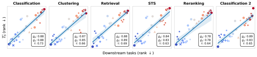
Figure 6: Correlations between rankings on different subtasks and their $\overline{\mathcal{I}_{S}}$ score ranking.

The strength of the MTEB benchmark is that it evaluates embedders on a very large and diverse set of downstream tasks. We provide an Tab. 4 and Figure 6 the full results of the MTEB benchmark (English) for the models used in the NLP experiments.

		$\varrho_{p}$	$\varrho_{s}$	$\tau$
Task category
Classification	Average	0.90	0.83	0.68
	AmazonCounterfactualClassification (en)	0.75	0.67	0.50
	AmazonPolarityClassification	0.78	0.77	0.58
	AmazonReviewsClassification (en)	0.83	0.82	0.65
	Banking77Classification	0.92	0.84	0.65
	EmotionClassification	0.87	0.76	0.58
	ImdbClassification	0.77	0.76	0.57
	MassiveIntentClassification (en)	0.93	0.84	0.68
	MassiveScenarioClassification (en)	0.92	0.84	0.67
	MTOPDomainClassification (en)	0.94	0.89	0.72
	MTOPIntentClassification (en)	0.80	0.76	0.59
	ToxicConversationsClassification	0.68	0.51	0.36
	TweetSentimentExtractionClassification	0.70	0.50	0.35
Clustering	Average	0.88	0.82	0.63
	ArxivClusteringP2P	0.59	0.64	0.46
	ArxivClusteringS2S	0.66	0.73	0.54
	BiorxivClusteringP2P	0.43	0.39	0.30
	BiorxivClusteringS2S	0.58	0.64	0.42
	MedrxivClusteringP2P	0.41	0.34	0.26
	MedrxivClusteringS2S	0.58	0.48	0.34
	RedditClustering	0.92	0.84	0.67
	RedditClusteringP2P	0.86	0.88	0.72
	StackExchangeClustering	0.93	0.88	0.71
	StackExchangeClusteringP2P	0.66	0.63	0.46
	TwentyNewsgroupsClustering	0.91	0.86	0.68
PairClassification	Average	0.91	0.83	0.67
	SprintDuplicateQuestions	0.69	0.63	0.44
	TwitterSemEval2015	0.92	0.76	0.57
	TwitterURLCorpus	0.85	0.81	0.64
Reranking	Average	0.85	0.74	0.58
	AskUbuntuDupQuestions	0.85	0.65	0.53
	MindSmallReranking	0.86	0.84	0.65
	SciDocsRR	0.63	0.50	0.35
	StackOverflowDupQuestions	0.89	0.77	0.58
Retrieval	Average	0.89	0.87	0.67
	ArguAna	0.80	0.77	0.59
	ClimateFEVER	0.75	0.78	0.59
	CQADupstackRetrieval	0.85	0.74	0.59
	DBPedia	0.94	0.90	0.74
	FEVER	0.87	0.86	0.67
	FiQA2018	0.85	0.74	0.57
	HotpotQA	0.88	0.87	0.69
	MSMARCO	0.84	0.78	0.60
	NFCorpus	0.91	0.86	0.68
	NQ	0.88	0.78	0.61
	QuoraRetrieval	0.90	0.80	0.63
	SCIDOCS	0.79	0.64	0.49
	SciFact	0.79	0.78	0.57
	Touche2020	0.71	0.58	0.41
	TRECCOVID	0.73	0.65	0.51
STS	Average	0.90	0.75	0.57
	STSBenchmark	0.85	0.70	0.53
	BIOSSES	0.80	0.72	0.52
	SICK-R	0.83	0.64	0.46
	STS12	0.80	0.63	0.44
	STS13	0.86	0.66	0.46
	STS14	0.89	0.68	0.47
	STS15	0.91	0.79	0.62
	STS16	0.91	0.76	0.59
	STS17 (en-en)	0.81	0.45	0.32
	STS22 (en)	0.84	0.61	0.45
Summarization	SummEval	0.46	0.31	0.21

Table 4: Detailed correlations between the $\overline{\mathcal{I}_{S}}$ score of the models and their performance on the MTEB benchmark.

We obtain significant positive correlations in all categories of downstream tasks. We noticed that we obtained significantly poorer results on STS, Clustering, and Reranking tasks than on classification tasks. We believe this behavior is due to the nature of these tasks. Indeed, they do not rely on training an additional model on top of the embeddings but rather directly use the embeddings as is in dot products or similarity measures. An embedder could produce very informative embeddings, i.e., it is possible to extract the useful information using a small model, and at the same time, these embeddings not be adequate for dot-product-based similarity measures. We believe further investigation is needed to understand the behavior of the models on these tasks. Especially to see if training a small model on top of the embeddings can improve the performance of these tasks.

C.3.2 Ablation studies

Many factors can impact the estimation of the $\overline{\mathcal{I}_{S}}$ score of the models, such as the dimensions of the different embeddings and the number of available embedders to evaluate. the $\overline{\mathcal{I}_{S}}$ score can capture many different aspects of the embeddings, such as the quality of the embeddings. We provide in this section a comprehensive set of ablation studies to evaluate the impact of these different factors on the $\overline{\mathcal{I}_{S}}$ score of the embeddings.

Impact of instruction finetuning.

Instruction finetuning is now a common practice to improve the alignment of the base of models and expand the models’ reasoning capabilities. In 4(c), show that instruction fine-tuning positively impacts the models’ performance on the downstream tasks and that the $\overline{\mathcal{I}_{S}}$ score captures this improvement. In addition to studying the impact of instruction finetuning, we evaluated models at different checkpoints during their initial pretraining in Sec. C.3.3 using the CroissantLLM checkpoints [37].

C.3.3 Impact of training steps

Surprisingly, we found that the number of training steps does not significantly impact the models’ performance on the downstream tasks nor on the $\overline{\mathcal{I}_{S}}$ score of the embeddings. The $\overline{\mathcal{I}_{S}}$ score correctly captures this behavior as shown in Figure 7. We hypothesize that the $\overline{\mathcal{I}_{S}}$ score in terms of embeddings is, in this case, determined by a few numbers of training steps (the first $5000$) and the overall architecture of the model. Training the model further even leads to a decrease in performance on the downstream tasks, which is not captured by the $\overline{\mathcal{I}_{S}}$ score of the embeddings; this could be due to the very small variation in the performance.

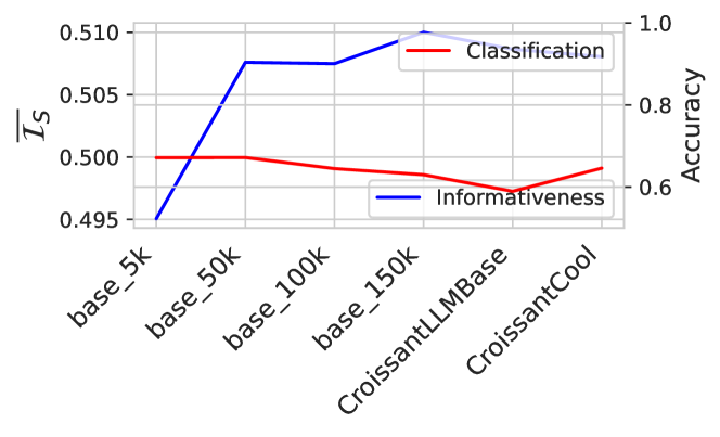
Figure 7: Impact of the number of training steps on the performance of the models on the downstream tasks and their $\overline{\mathcal{I}_{S}}$ score.

inforatmation sufficiency

C.3.4 Importance of embedding size normalization

We found that considering the amount of information packed by an embedding per coordinate is crucial to obtain a good ranking of the models. In 16(b), we show the correlation between the performance of the models on the MTEB benchmark and their $\overline{\mathcal{I}_{S}}$ score, not normalized by embedding size. While positive significative correlation is still present, the correlation is much weaker than when the dimension of the embeddings normalizes the information sufficiency.

C.3.5 Community and cluster performance

We postulate that models clustered together by information sufficiency are likely to behave similarly on the downstream tasks. We evaluate this hypothesis by grouping the models by clusters discovered using the information sufficiency and reporting their performance on the downstream tasks. In 8(b) and Figure 9, we observe that models within the same cluster tend to have similar behaviors on the downstream tasks.

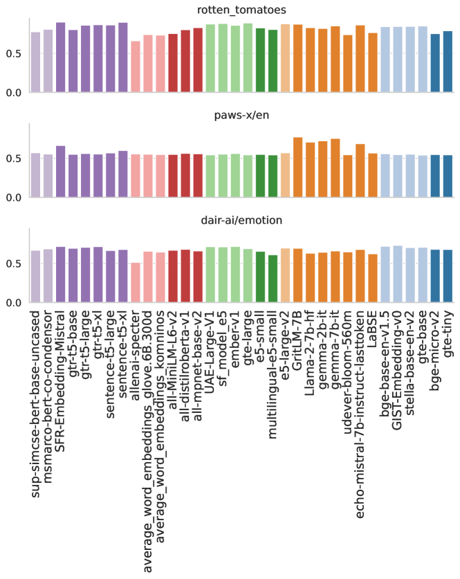
Figure 9: Performance of the models on the downstream tasks grouped by clusters discovered by the directed $\overline{\mathcal{I}_{S}}$.

C.3.6 Evaluating information sufficiency on different datasets

The $\overline{\mathcal{I}_{S}}$ score is evaluated with a fixed dataset supposed to represent the data distribution of interest (either a very diverse set or a subset following a distribution specific to a subfield like medical or legal texts). We cross-evaluated the $\overline{\mathcal{I}_{S}}$ of the models on different datasets and the performance of the models on the downstream tasks in Figure 10. We find that closer datasets in terms of the data distribution lead to a higher correlation between the $\overline{\mathcal{I}_{S}}$ score of the models and their performance on the downstream tasks. It is especially highlighted when comparing the correlations we get when evaluating $\overline{\mathcal{I}_{S}}$ on the AG News and Amazon polarity datasets. The first one corresponds to news articles, and the task is to guess the topic, whereas Amazon Polarity corresponds to product reviews, which is a sentiment analysis task. We find that the $\overline{\mathcal{I}_{S}}$ score evaluated on Amazon Polarity tends to yield way better correlation with the performance on the sentiment analysis downstream tasks such as tweet_eval/sentiment, tweet_eval/emotion, IMDB or Rotten Tomatoes or to a lesser extent dair/emotion. Interestingly, the difference is less significant on the tweet_eval/emoji subtask.

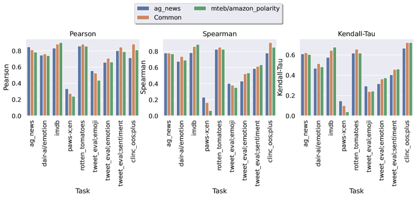
Figure 10: Correlation between $\overline{\mathcal{I}_{S}}$ scores computed on different datasets and the cross-performance on different tasks.

Appendix D Molecular Experiment Details

D.1 Embedders considered

Model name	SMILES	2D-GNN	3D-GNN	Architecture	Out size	Dataset (size)
Not-trained		✓		GIN	300	-
AttributeMask[99]		✓		GIN	300	GEOM [6] (50k)
ContextPred[99]		✓		GIN	300	GEOM [6] (50k)
GPT-GNN[48]		✓		GIN	300	GEOM [6] (50k)
InfoGraph[98]		✓		GIN	300	GEOM [6] (50k)
GraphCL[119]		✓		GIN	300	GEOM [6] (50k)
GROVER[89]		✓		GIN	300	GEOM [6] (50k)
GraphLog[116]		✓		GIN	300	GEOM [6] (50k)
GraphMVP[67]		✓		GIN	300	GEOM [6] (50k)
3D-infomax[96]		✓		PNA	800	QMugs [51] (620k)
MolR[112]		✓		GCN, GAT, TAG	1024	USPTO[112] ( 1.5M)
MoleOOD[117]		✓		GIN , SAGE, GCN	256	BACE [47] (400k)
ChemBERT MLM[3]	✓			RoBERTa	600	PubChem [55] (5M, 10M, 77M)
ChemBERT MTR[3]	✓			RoBERTa	384	PubChem [55] (5M, 10M, 77M)
MolBert[36]	✓			BERT	256	GuacaMol [18] (1.6M)
ChemGPT[40]	✓			GPT	128, 256, 2048	PubChem [55] (10M)
3D-denosing[121]			✓	TorchMD-net	256	PCQM4Mv2[46] (3.7M)
3D-fractional[39]			✓	TorchMD-net	256	PCQM4Mv2[46] (3.7M)

Table 5: Models evaluated on the ZINC dataset.

We considered $28$ models for the molecular experiments, summed up in Tab. 5. Some models were used in different versions (architectures, number of parameters, pretraining dataset’s size), such as the ChemBert models, followed by the size of their datasets, or ChemGPT, followed by their number of parameters.

Most 2D-GNNs were trained on the GEOM [6] dataset and were gathered from the repository of GraphMVP [67] model. Note that the MoleOOD [117] model was trained on the BACE [47] dataset, with a supervised task specific to the $\beta$-secretase enzyme. As a result, this model can be seen as "already specialized", explaining its poor performance in our evaluation.

We used the RD-Kit and Datamol tool-kits[61, 71] to pre-process the molecules and to generate three-dimensional conformers for 3D-models. To run the models using 3D views of the molecules, we generated five conformers (possible 3D configuration of the molecule) for each SMILES and kept the conformer with the lowest energy. Note that this methodology is imperfect, as the 3D coordinates might be noisy; however, we followed the same procedure to pre-process the ZINC dataset, to evaluate the information sufficiency, and on the datasets corresponding to each downstream task.

Finally we considered a variety of models architecture for 2D-GNNs notably graph isomorphism network (GIN) [115], principal neighbor aggregation networks (PNA) [26], graph convolutional network (GCN) [33], graph attention network (GAT) [110], topology adaptive graph convolutional networks (TAG) [32] and GraphSAGE [44]. For SMILES-based models, backbones are inspired by BERT [31], RoBERTa [69], and GPT [40]. Finally, both our 3D models use TorchMD-net[80] as a backbone.

D.2 Details on the information sufficiency estimation

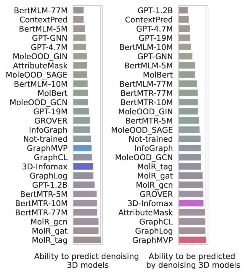
(a)

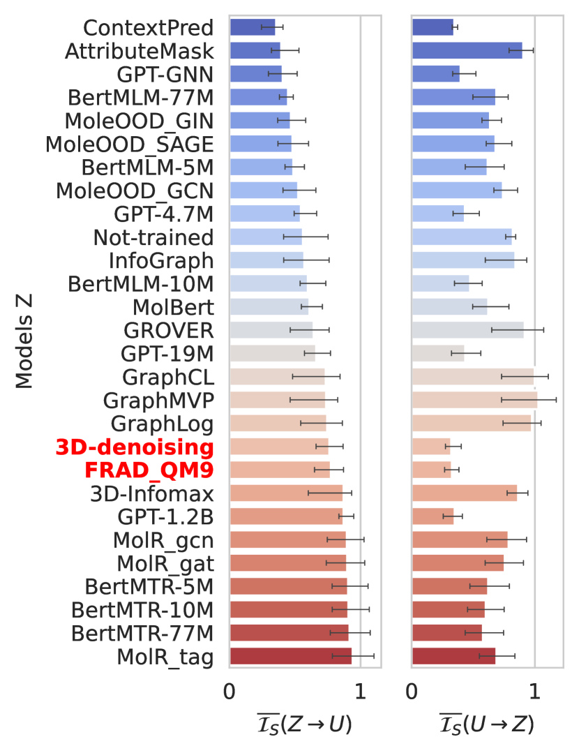
(b)

Figure 11: (a) Information sufficiency of embedders over 3D-Denoising models (left) and of 3D-Denoising models over the other embedders (right). (b) Information sufficiency of embedders in both directions. We see the 3D denoising models are among the least predicted models.

3D models. The two 3D models considered (FRAD [39] and Denoising [121]) obtain high $\overline{\mathcal{I}_{S}}$ scores while being among the least predictable (11(b) and Figure 12). This suggests that these models capture 3D-specific features inaccessible from other modalities while maintaining sufficient overlap to predict them.

2D-3D models Some 2D-GNNs we considered (GraphMVP and 3D-infomax) are trained to maximize the mutual information between their embeddings and 3D representations of the molecule. Hence, we expect these models to be related to the 3D-denoising models we considered. However, we observe in 11(a) that these models do not achieve particularly high information sufficiency scores over 3D-denoising models. On the other hand, the 3D models achieve high information sufficiency scores over them, which might suggest that these 2D models and 3D-denoising models share information that is easier to access from the 3D models. However, we want to point out that GraphMVP and 3D-infomax are both among the most predicted models; that is to say, among the other models in our pool, they achieve the highest information sufficiency scores.

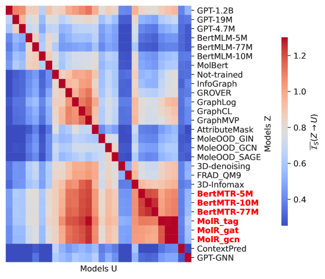
Figure 12: Pairwise information sufficiency between molecular embedders.

D.3 Complementary results on ADMET tasks

Category	Model	Task	cls	reg	Correlation			Avg. metric
	name	size			$\varrho_{p}$	$\varrho_{s}$	$\tau$	in the grid
Absorption	P-glycoprotein Inhibition	1212	✓		0.92	0.93	0.76	$0.88\pm 0.03$
	AqSolDB	9982		✓	0.91	0.91	0.75	$0.52\pm 0.09$
	Lipophilicity	4200		✓	0.88	0.89	0.71	$0.29\pm 0.07$
	Caco-2 Permeability	906		✓	0.77	0.80	0.61	$0.32\pm 0.08$
	Human Intestinal Absorption	578	✓		0.79	0.77	0.54	$0.67\pm 0.02$
	FreeSolv	642		✓	0.65	0.73	0.53	$0.36\pm 0.12$
	PAMPA Permeability	2035	✓		0.61	0.63	0.44	$0.67\pm 0.02$
	Oral Bioavailability	640	✓		0.50	0.45	0.33	$0.68\pm 0.02$
Distribution	Plasma-Protein BDR	1614		✓	0.85	0.84	0.68	$0.18\pm 0.04$
	Blood-Brain barrier	1975	✓		0.79	0.81	0.60	$0.32\pm 0.08$
	VDss	1130		✓	0.71	0.73	0.53	$0.16\pm 0.05$
Metabolism	CYPP450 3A4 Inhib.	12328	✓		0.96	0.96	0.85	$0.80\pm 0.04$
	CYPP450 1A2 Inhib.	12579	✓		0.94	0.95	0.81	$0.87\pm 0.03$
	CYPP450 2C19 Inhib.	12665	✓		0.94	0.95	0.75	$0.82\pm 0.03$
	CYPP450 2C9 Inhib.	12092	✓		0.92	0.92	0.79	$0.83\pm 0.03$
	CYPP450 2D6 Inhib.	13130	✓		0.94	0.91	0.74	$0.78\pm 0.04$
	CYPP450 2D6 Substrate	664	✓		0.75	0.74	0.57	$0.75\pm 0.03$
	CYPP450 3A4 Substrate	667	✓		0.50	0.53	0.35	$0.63\pm 0.02$
	CYPP450 2C9 Substrate	666	✓		0.20	0.13	0.09	$0.65\pm 0.02$
Excretion	Clearance hepatocyte	1020		✓	0.78	0.79	0.57	$0.11\pm 0.03$
	Half Life	667		✓	0.76	0.78	0.58	$-0.06\pm 0.11$
	Clearance microsome	1102		✓	0.72	0.72	0.54	$0.08\pm 0.03$
Toxicity	Tox21	7831	✓		0.93	0.93	0.78	$0.75\pm 0.03$
	hERG	13445	✓		0.91	0.90	0.75	$0.76\pm 0.04$
		648	✓		0.81	0.84	0.63	$0.75\pm 0.03$
	Acute Toxicity LD50	7385		✓	0.82	0.82	0.63	$0.16\pm 0.04$
	Ames Mutagenicity	7255	✓		0.79	0.78	0.60	$0.79\pm 0.03$
	ClinTox	1484	✓		0.69	0.69	0.49	$0.71\pm 0.03$
	Carcinogens	278	✓		0.47	0.49	0.35	$0.76\pm 0.08$
	Drug Induced Liver Injury	475	✓		0.39	0.36	0.25	$0.83\pm 0.03$
	Skin Reaction	404	✓		0.01	0.07	0.06	$0.64\pm 0.03$

Table 6: ADMET tasks extracted from the Therapeutic Data Commons platform [49] considered in our experiments. We report the correlation between the informativeness score and the performances of the embedders on the downstream tasks in terms of Pearson correlation $\varrho_{p}$, Spearman correlation $\varrho_{s}$ and Kendall-Tau $\tau$. We also report the average metric of the models on each task across the grid search runs, in terms of $R^{2}$ for regression tasks and AUROC for classification tasks. The tasks are ordered within each category by the correlation with the informativness score (in terms of Spearman correlation).

The datasets chosen for the molecular experiments are extracted from the Therapeutics Data Commons (TDC) [49] platform. We focused our experiments on ADMET tasks, crucial for drug discovery and development, which results in a total of $31$ tasks, described in Tab. 6.

Dropout rate	hidden dimension	network depth	n-epochs
$0$, $0.2$	$4$, $8$, $16$, $32$, $64$, $128$	$1$, $2$, $3$	min$(200,200*\frac{5000}{\text{task size}})$

Table 7: Hyperparameters tuned for the evaluation of embedders on ADMET downstream tasks

Each dataset is split into a training set, a validation set, and a test set following a scaffold split. This splitting strategy ensures that molecules sharing a similar scaffold will be part of the same split in the task. This corresponds to a more realistic scenario, where practitioners only have access to molecules belonging to the same chemical series. Classifiers are then trained on the training set of each task, where the best hyperparameters and checkpoints are selected on the validation set. The final performance is finally measured on the test set, and we run each experiment $10$ times with different random seeds.

A grid search is performed on each dataset individually to maximize the average AUROC or $R^{2}$ score across all models for binary classification and regression. We chose a maximum number of epochs depending on the task size to ensure all models have time to converge, limiting this amount to grow to at most $200$ epochs.

Tab. 6 also displays the variation of the correlation coefficient between the ranking obtained on the $\overline{\mathcal{I}_{S}}$ score and the performances obtained on the downstream tasks regarding Spearman and Kendall correlations. We can see that the $\overline{\mathcal{I}_{S}}$ score correlates well with the performance of downstream tasks when the amount of data available is large.

Finally, we can see in Figure 13 that by grouping models based on their performances on these tasks, we obtain a similar clustering to the one obtained on the $\overline{\mathcal{I}_{S}}$ score in Sec. 6.2, with NLP-inspired models grouped. Similarly, the tinyChemBert-MTR and MolR models are also grouped.

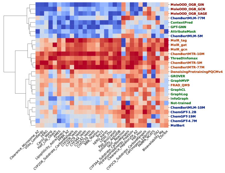
Figure 13: Heatmap representation of the performances of the different models on the downstream tasks, where embedders behaving similarly on the various tasks are clustered, and the embedders are colored based on their community computed in Sec. 6.2 based on the $\overline{\mathcal{I}_{S}}$ score.

D.4 Drug target Interaction prediction

Figure 14: Correlations of the $\overline{\mathcal{I}_{S}}$ score with the performances on the DTI tasks, in terms of Spearman and Kendall coefficients.

We propose further evaluating the embedders on yet another type of downstream task: Drug-Target Interaction. This task aims to predict the binding affinity between a given pair (drug, target). Since none of our models can process protein sequences, we decompose each dataset into multiple regression tasks on a single target by querying all molecules associated with a label for this target. Each task is then formulated as a set of molecules: $\mathcal{X}=\{x_{i}\}_{i\in\{0,\ldots,N\}}$, and their labels $\mathcal{Y}=\{y_{i}\}_{i\in\{0,\ldots,N\}}$

However, such tasks can be small, making it hard to build proper models from the embeddings. In contrast, the number of tasks is very large, making it computationally expensive to proceed to an adequate hyperparameter selection. To bypass these limitations, we propose to estimate the embedded space’s clustering quality for each model by measuring how close the labels of a molecule are compared to its nearest neighbors for each task. In other words, we measure:

$$\tilde{\mathcal{L}}_{n_{\textrm{neigh}}}(\mathcal{X},\mathcal{Y}) =\frac{1}{N}\sum_{i=0}^{N}\mathcal{L}_{n_{\textrm{neigh}}}(i,\mathcal{X},\mathcal{Y}),$$ (22)

$$\text{with}\quad\mathcal{L}_{n_{\textrm{neigh}}}(i,\mathcal{X},\mathcal{Y}) =\frac{1}{n_{\textrm{neigh}}}\sum_{j\in\mathcal{N}_{i,n_{\textrm{neigh}}}(\mathcal{X})}\lVert y_{i}-y_{j}\rVert^{2},$$

and $\mathcal{N}_{i,n_{\textrm{neigh}}}(\mathcal{X})$ is the set containing the $n_{\textrm{neigh}}$ closest neighbors of $x_{i}\in\mathcal{X}$, which would be the performances of a K-nearest neighbors regressor on the task when using one data sample.

This quantity can be interpreted as a proxy of the embedding’s capability to perform a similarity search, a classic chemo-informatic method using the similarity between different molecular projections to perform predictions. This training-free and computationally inexpensive approach allows us to evaluate the models on many tasks/targets.

We focused on 4 DTI datasets: KIBA [101], BindingDB-Kd, BindingDB-Ki, and BindingDB-IC50 [68], with a total of $1496$ tasks. We removed all tasks containing less than 128 molecules to ensure minimum data for the clustering evaluation.

	KIBA (175 targets)				BindingDB-Kd (22 targets)				BindingDB-Ki (372 targets)				BindingDB-IC50 (927 targets)
$n_{neighb}$	1	2	4	8	1	2	4	8	1	2	4	8	1	2	4	8
$\varrho_{p}$	0.85	0.84	0.84	0.83	0.90	0.90	0.87	0.84	0.88	0.88	0.88	0.87	0.87	0.86	0.86	0.86
$\varrho_{s}$	0.88	0.88	0.87	0.86	0.87	0.86	0.85	0.82	0.87	0.87	0.87	0.88	0.86	0.87	0.87	0.86
$\tau$	0.72	0.71	0.69	0.67	0.68	0.66	0.65	0.62	0.68	0.67	0.69	0.69	0.66	0.68	0.69	0.68

Table 8: Correlation between $\overline{\mathcal{I}_{S}}$’s informativness score and our clustering evaluation score $\tilde{\mathcal{L}}_{n_{\textrm{neighb}}}$ on the four DTI datasets considered.

We obtain similar results as in Sec. 6.1, our metric correlating with the performances on the different tasks considered. Figure 14 sums up all results by establishing a ranking across models and the number of neighbors, where we can see that MolR and ChemBerta-MTR appear as both the most promising models according to their $\overline{\mathcal{I}_{S}}$ score, and the best models evaluated. Furthermore, the outliers observed inSec. 6.1 show different behaviors in this setting. For instance, while 3D-Infomax seemed under-estimated and InfoGraph over-estimated by the $\overline{\mathcal{I}_{S}}$ score after seeing the results on the ADMET tasks, Infograph appears under-estimated in this setup, and 3D-infomax over-estimated.

Appendix E Information Sufficiency Estimation

E.1 Estimation method

As stated in Sec. 2, the deficiency $\delta(P_{U|X}\rightarrow P_{Z|X})$ is an intractable object measuring the cost of the reconstruction of $Z$ from $U$. Due to this intractability, we propose to estimate the information sufficiency $\mathcal{I}_{S}(U\rightarrow Z)$, which is a tractable proxy for the deficiency.

Embedding dimension normalization.

However, this approach faces one major drawback: it favors models that generate embeddings of high dimensionality. To evaluate the information sufficiency between the models, we estimate the uncertainty of $Z$ and the uncertainty of $Z$ given $U$. As seen in Figure 15, the estimated information sufficiency is highly correlated to the dimension of the latent space of $Z$, favoring models with high-dimensional latent spaces. This can be explained by the fact that these embedders yield larger marginal uncertainties. The resulting difference in the uncertainties $\mathcal{I}_{S}(U\rightarrow Z)$ is hence larger in absolute values.

We can see in Figure 15 that the dimension of the latent space of $Z$ and the uncertainty of $Z$ are evolving linearly. We thereby divide the information sufficiency by $dim(Z)$, which can be seen as an approximation of the normalization by the uncertainty of $Z$. We report in 16(b) results without this normalization. It still correlates significantly with the downstream tasks performance, but the correlation is stronger when the normalization is applied. Hence, we focus on the relative variation of the uncertainty of $Z$ explained by $U$. Note that the uncertainty of $Z$ can be negative, as it can be assimilated to a differential entropy. As a result, the “true“ relative variation of the uncertainty would not be suitable for comparing different models (as it would not guarantee any ordering). While there is a general trend where larger models do have larger embeddings and perform better, well-trained smaller embeddings are competitive with larger embeddings, and the $\overline{\mathcal{I}_{S}}$ score captures this behavior (16(a)).

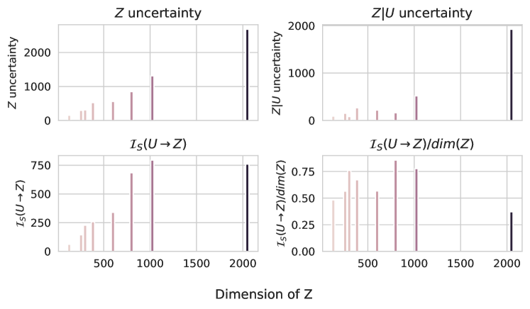
Figure 15: Relationship between the dimension of $Z$’s latent space and the quantities estimated to compute the information sufficiency in molecular modeling.

We build our proxy by measuring the median values of the set $\mathcal{S}_{\mathcal{I_{S}}}\left(k\right)=\left\{\mathcal{I}_{S}(Z_{k}\rightarrow Z_{l})\right\}_{l\not=k}$ for an embedder $Z_{k}$ in our pool of models.

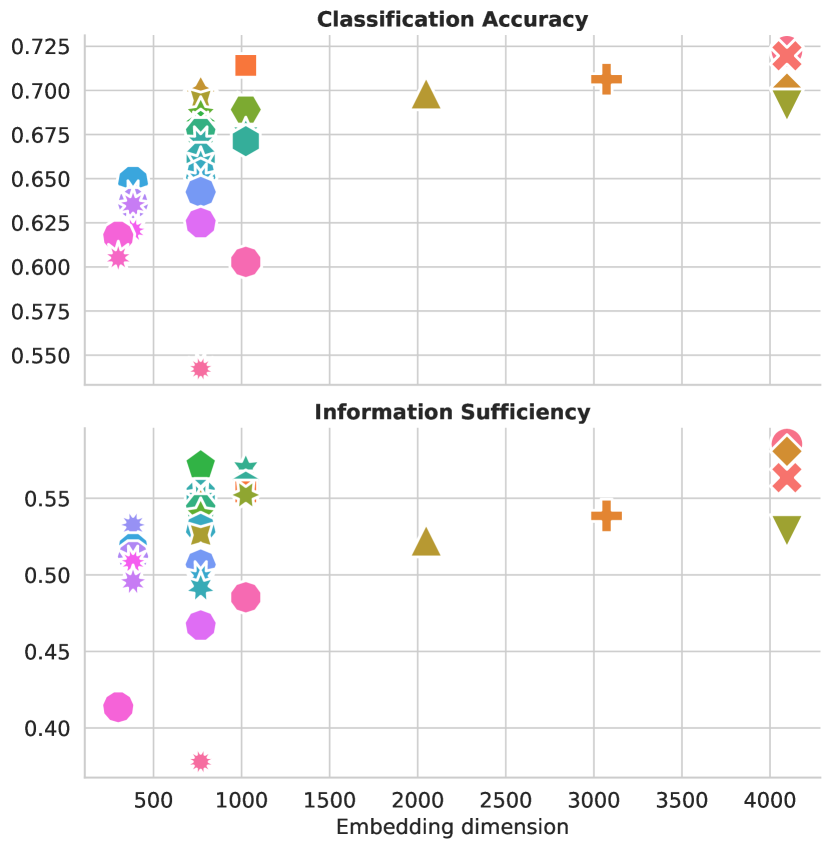
(a) Impact of the embedding size on the quality of the embeddings for the models measured as actual performance on downstream tasks and $\overline{\mathcal{I}_{S}}$ score.

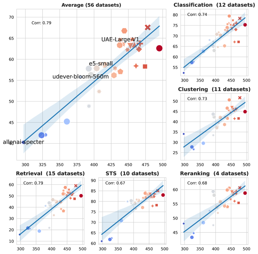
(b) Correlations on the MTEB benchmark when the embeddings are not normalized by their size.

Figure 16:

Median instead of mean.

We use the median instead of the mean to compute the $\overline{\mathcal{I}_{S}}$ score. The median is more robust to outliers and the distribution of available embedders. For example, if many models are very similar, the mean would be biased by these models, while the median would not. Thus, we chose the median. While this change has a minor impact when there is enough diversity in the models, it can have a significant impact when the models are very similar, for example, when including different checkpoints of the same model Figure 17.

	$\varrho_{p}$	$\varrho_{s}$	$\tau$
STS (10 datasets)	0.90	0.85	0.66
Retrieval (15 datasets)	0.89	0.85	0.62
Classification (12 datasets)	0.92	0.84	0.65
Clustering (11 datasets)	0.86	0.83	0.61
Reranking (4 datasets)	0.86	0.79	0.65
Average (56 datasets)	0.93	0.86	0.66
Additional Classif (8 datasets)	0.84	0.81	0.61

(a) NLP

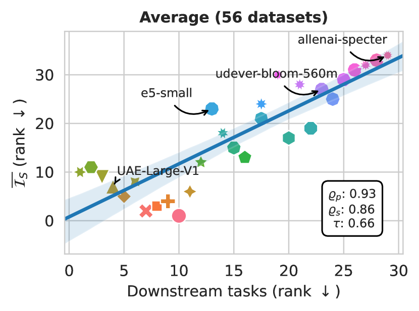
(a) NLP

Figure 17: Correlation between $\overline{\mathcal{I}_{S}}$ score computed as the mean information sufficiency and the downstream task performances in NLP. $\varrho_{p}$ is the Pearson correlation, $\varrho_{s}$ is the spearman correlation

E.2 Hyperparameter selection

We use parametric classes composed of multivariate Gaussian mixture distributions for $\mathcal{F}_{\Theta}$ and $\mathcal{K}_{\Theta}(\mathsf{Z}|\mathsf{U})$ in the definition of the information sufficiency (Eq. 1), the number of components in the mixture is a crucial parameter that needs to be selected concerning the data distribution of interest. We ran ablation studies to evaluate the impact of the number of components in the mixture on the information sufficiency estimation and the correlation between the $\overline{\mathcal{I}_{S}}$ score and the downstream tasks performance (Figure 20). We found that the ideal number of components in NLP is $8$, and in molecular modeling, it is $4$. Figure 18 and Figure 19 show the embeddings of the models in the first two principal components.

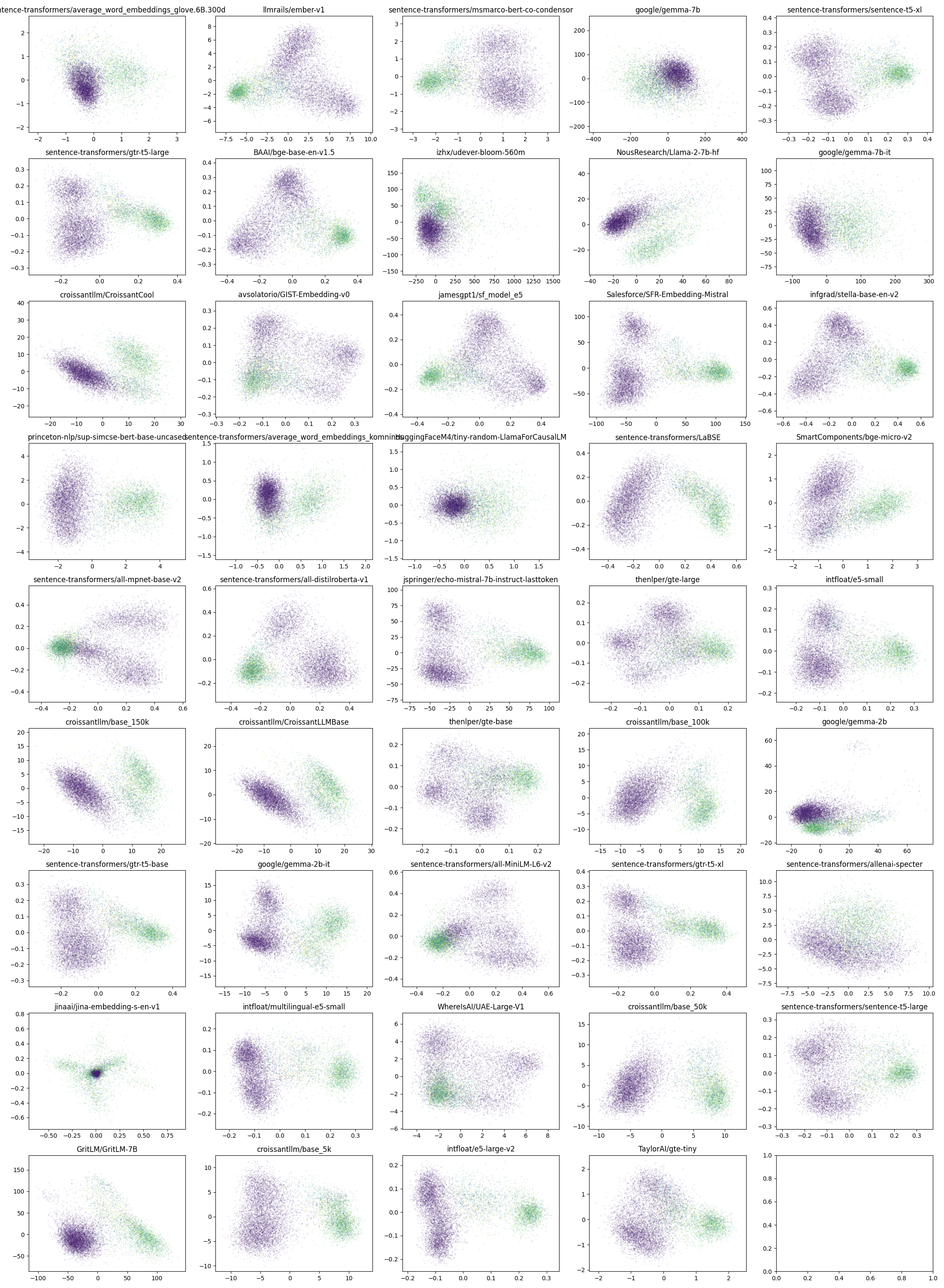
Figure 18: 2D Projection of the embeddings of the models in the first two principal components colored by datasets in NLP

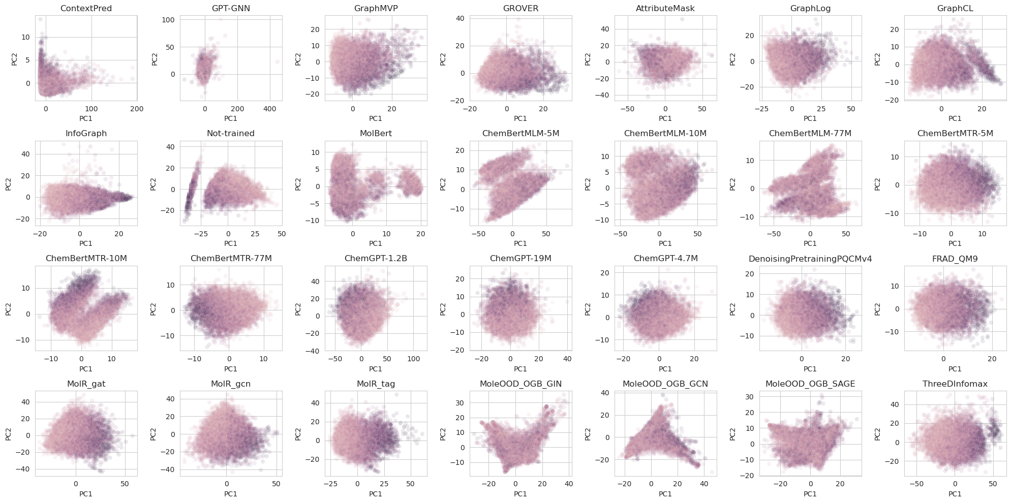
Figure 19: 2D Projection of the embeddings of the models in the first two principal components colored by datasets in molecular modeling. Hue corresponds to the synthetic accessibility score [34].

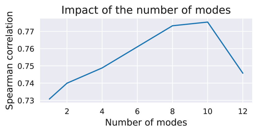
(a) Spearman

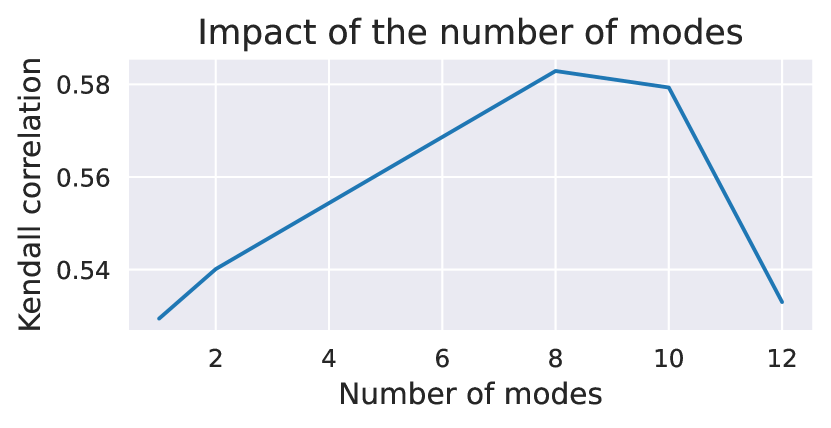
(b) Kendall-Tau.

(c) Pearson.

Figure 20: Impact of the number of modes used to estimate the $\overline{\mathcal{I}_{S}}$ score and its correlation with the downstream tasks performance in NLP. We chose to use $8$ modes in practice.

E.3 Impact of the task size

Our study focused on finding the most promising model to be competitive on any downstream tasks. However, if the downstream task is not learnable, the most promising model could appear as not competitive on this specific task. In particular, if the amount of data available in the downstream task is insufficient, the differences between different embedder’s representations might not be easily leveraged. This phenomenon can be seen in Figure 21, highlighting how when fewer than 1000 data points are available, the correlation between the $\overline{\mathcal{I}_{S}}$ score and the downstream performance becomes weaker.

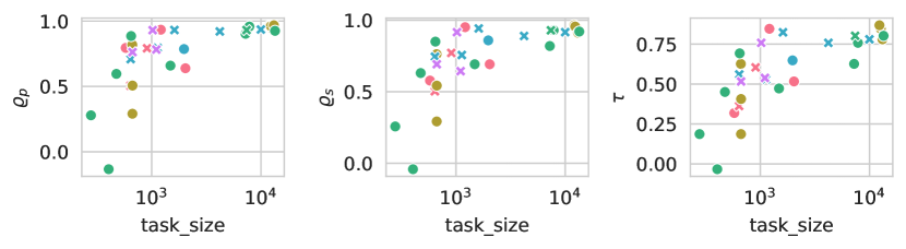
Figure 21: Impact of the task size on the $\overline{\mathcal{I}_{S}}$ score’s ranking’s correlation with the downstream tasks performances in molecular modeling in terms of Pearson correlation $\varrho_{p}$, Spearman correlation $\varrho_{s}$ and Kendall-Tau $\tau$ coefficient.

E.4 Impact of the number of models

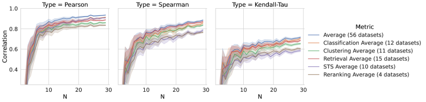
Figure 22: Impact of the number of models used to compute the $\overline{\mathcal{I}_{S}}$ score in NLP.

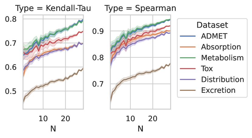
Figure 23: Impact of the number of models used to compute the $\overline{\mathcal{I}_{S}}$ score in molecular modeling.

We evaluate the strength or $\overline{\mathcal{I}_{S}}$ score of an embedder with respect to all the others by relaxing the "for all" conditions with the median $\overline{\mathcal{I}_{S}}$ score. Thus, the number of available embedders might impact the performance of our method. Indeed, if too few embedders are available, it is likely that our evaluation would be biased by favoring models similar to the few available ones. We evaluate the impact of the number of available models by sampling subsets of our global model pool to compute the $\overline{\mathcal{I}_{S}}$ score. In Figure 22, we found that when fewer models are available, the rankings obtained using the $\overline{\mathcal{I}_{S}}$ score correlate less with the downstream tasks’ performance. However, as the number of models increases, the $\overline{\mathcal{I}_{S}}$ score becomes a good proxy for the performance of the models on the downstream tasks.

However, the evolution of this correlation is different in the two studied domains. Even with very few models, the $\overline{\mathcal{I}_{S}}$ score of molecular models already achieves a Spearman correlation close to $0.8$ with the downstream tasks’ performance. The correlation is much lower in NLP and only reaches $0.8$ when about $15$ models are available. This result can be expected, seeing how sparse the pairwise comparison matrix is in NLP compared to molecular modeling. This matrix is less sparse on molecular data, the graph induced by this adjacency matrix is more connected, and having access to a few nodes is enough to obtain measurements on the whole graph. On the contrary, by being much sparser, having access to a few nodes in this graph in NLP might only give information about the local structure of the graph in the community of the few nodes available. This might explain why the $\overline{\mathcal{I}_{S}}$ score’s correlation with the downstream tasks performance stabilizes in NLP at about ten models, which is equal to the number of communities identified in the graph (in Sec. 5.2).

E.5 Computational ressources

Evaluating the $\overline{\mathcal{I}_{S}}$ score of the models is computationally inexpensive. Evaluating the $\overline{\mathcal{I}_{S}}$ score requires only a single (small) GPU. All our experiments were conducted on NVIDIA V100 and NVIDIA A6000 GPUs.

Our method’s main (computational) shortcoming stems from the need to compute the information sufficiency between all pairs of models. This is a quadratic operation in the number of models. However, in practice, optimizing and estimating the information sufficiency presented in Sec. 3 is cheap. The complete evaluation of the $45$ NLP models can be done in less than $6$ hours on a single GPU.

NeurIPS Paper Checklist

1. Claims

2. Question: Do the main claims made in the abstract and introduction accurately reflect the paper’s contributions and scope?

3. Answer: [Yes]

4. Justification: We setup the problem of evaluating embedders as a communication problem and leverage information theoretic tools to derive a principled evaluation method.

5. Guidelines:

   • The answer NA means that the abstract and introduction do not include the claims made in the paper.

   • The abstract and/or introduction should clearly state the claims made, including the contributions made in the paper and important assumptions and limitations. A No or NA answer to this question will not be perceived well by the reviewers.

   • The claims made should match theoretical and experimental results, and reflect how much the results can be expected to generalize to other settings.

   • It is fine to include aspirational goals as motivation as long as it is clear that these goals are not attained by the paper.

6. Limitations

7. Question: Does the paper discuss the limitations of the work performed by the authors?

8. Answer: [Yes]

9. Justification: We provide a separate section "Conclusion and Limitations" (Sec. 7) in the main paper and different ablations addressing possible shortcomings of our methods in appendices.

10. Guidelines:

    • The answer NA means that the paper has no limitation while the answer No means that the paper has limitations, but those are not discussed in the paper.

    • The authors are encouraged to create a separate "Limitations" section in their paper.

    • The paper should point out any strong assumptions and how robust the results are to violations of these assumptions (e.g., independence assumptions, noiseless settings, model well-specification, asymptotic approximations only holding locally). The authors should reflect on how these assumptions might be violated in practice and what the implications would be.

    • The authors should reflect on the scope of the claims made, e.g., if the approach was only tested on a few datasets or with a few runs. In general, empirical results often depend on implicit assumptions, which should be articulated.

    • The authors should reflect on the factors that influence the performance of the approach. For example, a facial recognition algorithm may perform poorly when image resolution is low or images are taken in low lighting. Or a speech-to-text system might not be used reliably to provide closed captions for online lectures because it fails to handle technical jargon.

    • The authors should discuss the computational efficiency of the proposed algorithms and how they scale with dataset size.

    • If applicable, the authors should discuss possible limitations of their approach to address problems of privacy and fairness.

    • While the authors might fear that complete honesty about limitations might be used by reviewers as grounds for rejection, a worse outcome might be that reviewers discover limitations that aren’t acknowledged in the paper. The authors should use their best judgment and recognize that individual actions in favor of transparency play an important role in developing norms that preserve the integrity of the community. Reviewers will be specifically instructed to not penalize honesty concerning limitations.

11. Theory Assumptions and Proofs

12. Question: For each theoretical result, does the paper provide the full set of assumptions and a complete (and correct) proof?

13. Answer: [Yes]

14. Justification: We provide a complete description of our setting and assumptions used to derive theoretical proofs as well, as the relaxation of the problem to make it tractable (Sec. 2, Appendix B).

15. Guidelines:

    • The answer NA means that the paper does not include theoretical results.

    • All the theorems, formulas, and proofs in the paper should be numbered and cross-referenced.

    • All assumptions should be clearly stated or referenced in the statement of any theorems.

    • The proofs can either appear in the main paper or the supplemental material, but if they appear in the supplemental material, the authors are encouraged to provide a short proof sketch to provide intuition.

    • Inversely, any informal proof provided in the core of the paper should be complemented by formal proofs provided in appendix or supplemental material.

    • Theorems and Lemmas that the proof relies upon should be properly referenced.

16. Experimental Result Reproducibility

17. Question: Does the paper fully disclose all the information needed to reproduce the main experimental results of the paper to the extent that it affects the main claims and/or conclusions of the paper (regardless of whether the code and data are provided or not)?

18. Answer: [Yes]

19. Justification: We provide a description of our global experimental protocol in the main paper (Sec. 4) and detailed descriptions for the different field in their respective sections (Appendix C, Appendix D). All the datasets and models used are publicly available and the code to reproduce our results is attached to the submission.

20. Guidelines:

    • The answer NA means that the paper does not include experiments.

    • If the paper includes experiments, a No answer to this question will not be perceived well by the reviewers: Making the paper reproducible is important, regardless of whether the code and data are provided or not.

    • If the contribution is a dataset and/or model, the authors should describe the steps taken to make their results reproducible or verifiable.

    • Depending on the contribution, reproducibility can be accomplished in various ways. For example, if the contribution is a novel architecture, describing the architecture fully might suffice, or if the contribution is a specific model and empirical evaluation, it may be necessary to either make it possible for others to replicate the model with the same dataset, or provide access to the model. In general. releasing code and data is often one good way to accomplish this, but reproducibility can also be provided via detailed instructions for how to replicate the results, access to a hosted model (e.g., in the case of a large language model), releasing of a model checkpoint, or other means that are appropriate to the research performed.

    • While NeurIPS does not require releasing code, the conference does require all submissions to provide some reasonable avenue for reproducibility, which may depend on the nature of the contribution. For example

      1. If the contribution is primarily a new algorithm, the paper should make it clear how to reproduce that algorithm.

      2. If the contribution is primarily a new model architecture, the paper should describe the architecture clearly and fully.

      3. If the contribution is a new model (e.g., a large language model), then there should either be a way to access this model for reproducing the results or a way to reproduce the model (e.g., with an open-source dataset or instructions for how to construct the dataset).

      4. We recognize that reproducibility may be tricky in some cases, in which case authors are welcome to describe the particular way they provide for reproducibility. In the case of closed-source models, it may be that access to the model is limited in some way (e.g., to registered users), but it should be possible for other researchers to have some path to reproducing or verifying the results.

21. Open access to data and code

22. Question: Does the paper provide open access to the data and code, with sufficient instructions to faithfully reproduce the main experimental results, as described in supplemental material?

23. Answer: [Yes]

24. Justification: We attached the code to the submission and provide instructions to reproduce the results in the main paper and supplemental material. All datasets and models are publicly available and chosen to be easily accessible for reproducibility.

25. Guidelines:

    • The answer NA means that paper does not include experiments requiring code.

    • Please see the NeurIPS code and data submission guidelines (https://nips.cc/public/guides/CodeSubmissionPolicy) for more details.

    • While we encourage the release of code and data, we understand that this might not be possible, so “No” is an acceptable answer. Papers cannot be rejected simply for not including code, unless this is central to the contribution (e.g., for a new open-source benchmark).

    • The instructions should contain the exact command and environment needed to run to reproduce the results. See the NeurIPS code and data submission guidelines (https://nips.cc/public/guides/CodeSubmissionPolicy) for more details.

    • The authors should provide instructions on data access and preparation, including how to access the raw data, preprocessed data, intermediate data, and generated data, etc.

    • The authors should provide scripts to reproduce all experimental results for the new proposed method and baselines. If only a subset of experiments are reproducible, they should state which ones are omitted from the script and why.

    • At submission time, to preserve anonymity, the authors should release anonymized versions (if applicable).

    • Providing as much information as possible in supplemental material (appended to the paper) is recommended, but including URLs to data and code is permitted.

26. Experimental Setting/Details

27. Question: Does the paper specify all the training and test details (e.g., data splits, hyperparameters, how they were chosen, type of optimizer, etc.) necessary to understand the results?

28. Answer: [Yes]

29. Justification: We provide in Appendix Appendix C and Appendix D the details of the training and test settings for the different fields. We also provide a global description of the experimental protocol in the main paper (Sec. 4).

30. Guidelines:

    • The answer NA means that the paper does not include experiments.

    • The experimental setting should be presented in the core of the paper to a level of detail that is necessary to appreciate the results and make sense of them.

    • The full details can be provided either with the code, in appendix, or as supplemental material.

31. Experiment Statistical Significance

32. Question: Does the paper report error bars suitably and correctly defined or other appropriate information about the statistical significance of the experiments?

33. Answer: [Yes]

34. Justification: We provide error bars in the figures and tables of the main paper. In addition we provide robustness checks and ablations in the appendices.

35. Guidelines:

    • The answer NA means that the paper does not include experiments.

    • The authors should answer "Yes" if the results are accompanied by error bars, confidence intervals, or statistical significance tests, at least for the experiments that support the main claims of the paper.

    • The factors of variability that the error bars are capturing should be clearly stated (for example, train/test split, initialization, random drawing of some parameter, or overall run with given experimental conditions).

    • The method for calculating the error bars should be explained (closed form formula, call to a library function, bootstrap, etc.)

    • The assumptions made should be given (e.g., Normally distributed errors).

    • It should be clear whether the error bar is the standard deviation or the standard error of the mean.

    • It is OK to report 1-sigma error bars, but one should state it. The authors should preferably report a 2-sigma error bar than state that they have a 96% CI, if the hypothesis of Normality of errors is not verified.

    • For asymmetric distributions, the authors should be careful not to show in tables or figures symmetric error bars that would yield results that are out of range (e.g. negative error rates).

    • If error bars are reported in tables or plots, The authors should explain in the text how they were calculated and reference the corresponding figures or tables in the text.

36. Experiments Compute Resources

37. Question: For each experiment, does the paper provide sufficient information on the computer resources (type of compute workers, memory, time of execution) needed to reproduce the experiments?

38. Answer: [Yes]

39. Justification: We provide the details of the compute resources used in the main paper and appendices in Sec. E.5.

40. Guidelines:

    • The answer NA means that the paper does not include experiments.

    • The paper should indicate the type of compute workers CPU or GPU, internal cluster, or cloud provider, including relevant memory and storage.

    • The paper should provide the amount of compute required for each of the individual experimental runs as well as estimate the total compute.

    • The paper should disclose whether the full research project required more compute than the experiments reported in the paper (e.g., preliminary or failed experiments that didn’t make it into the paper).

41. Code Of Ethics

42. Question: Does the research conducted in the paper conform, in every respect, with the NeurIPS Code of Ethics https://neurips.cc/public/EthicsGuidelines?

43. Answer: [Yes]

44. Justification: This paper does not involve major ethical concerns and the research conducted in the paper conforms with the NeurIPS Code of Ethics.

45. Guidelines:

    • The answer NA means that the authors have not reviewed the NeurIPS Code of Ethics.

    • If the authors answer No, they should explain the special circumstances that require a deviation from the Code of Ethics.

    • The authors should make sure to preserve anonymity (e.g., if there is a special consideration due to laws or regulations in their jurisdiction).

46. Broader Impacts

47. Question: Does the paper discuss both potential positive societal impacts and negative societal impacts of the work performed?

48. Answer: [N/A]

49. Justification: We only propose model selection method for embedders. The main concern, that is addressed in the paper, is that while our method is theoretically supported and empirically validated, it might not be applicable to all downstream tasks and should be used with caution.

50. Guidelines:

    • The answer NA means that there is no societal impact of the work performed.

    • If the authors answer NA or No, they should explain why their work has no societal impact or why the paper does not address societal impact.

    • Examples of negative societal impacts include potential malicious or unintended uses (e.g., disinformation, generating fake profiles, surveillance), fairness considerations (e.g., deployment of technologies that could make decisions that unfairly impact specific groups), privacy considerations, and security considerations.

    • The conference expects that many papers will be foundational research and not tied to particular applications, let alone deployments. However, if there is a direct path to any negative applications, the authors should point it out. For example, it is legitimate to point out that an improvement in the quality of generative models could be used to generate deepfakes for disinformation. On the other hand, it is not needed to point out that a generic algorithm for optimizing neural networks could enable people to train models that generate Deepfakes faster.

    • The authors should consider possible harms that could arise when the technology is being used as intended and functioning correctly, harms that could arise when the technology is being used as intended but gives incorrect results, and harms following from (intentional or unintentional) misuse of the technology.

    • If there are negative societal impacts, the authors could also discuss possible mitigation strategies (e.g., gated release of models, providing defenses in addition to attacks, mechanisms for monitoring misuse, mechanisms to monitor how a system learns from feedback over time, improving the efficiency and accessibility of ML).

51. Safeguards

52. Question: Does the paper describe safeguards that have been put in place for responsible release of data or models that have a high risk for misuse (e.g., pretrained language models, image generators, or scraped datasets)?

53. Answer: [N/A]

54. Justification: N/A

55. Guidelines:

    • The answer NA means that the paper poses no such risks.

    • Released models that have a high risk for misuse or dual-use should be released with necessary safeguards to allow for controlled use of the model, for example by requiring that users adhere to usage guidelines or restrictions to access the model or implementing safety filters.

    • Datasets that have been scraped from the Internet could pose safety risks. The authors should describe how they avoided releasing unsafe images.

    • We recognize that providing effective safeguards is challenging, and many papers do not require this, but we encourage authors to take this into account and make a best faith effort.

56. Licenses for existing assets

57. Question: Are the creators or original owners of assets (e.g., code, data, models), used in the paper, properly credited and are the license and terms of use explicitly mentioned and properly respected?

58. Answer: [Yes]

59. Justification: We provide the citations and direct references of all the datasets and models used in our work. To ensure reproducibility, all the datasets and models used are publicly available and under open licenses.

60. Guidelines:

    • The answer NA means that the paper does not use existing assets.

    • The authors should cite the original paper that produced the code package or dataset.

    • The authors should state which version of the asset is used and, if possible, include a URL.

    • The name of the license (e.g., CC-BY 4.0) should be included for each asset.

    • For scraped data from a particular source (e.g., website), the copyright and terms of service of that source should be provided.

    • If assets are released, the license, copyright information, and terms of use in the package should be provided. For popular datasets, paperswithcode.com/datasets has curated licenses for some datasets. Their licensing guide can help determine the license of a dataset.

    • For existing datasets that are re-packaged, both the original license and the license of the derived asset (if it has changed) should be provided.

    • If this information is not available online, the authors are encouraged to reach out to the asset’s creators.

61. New Assets

62. Question: Are new assets introduced in the paper well documented and is the documentation provided alongside the assets?

63. Answer: [Yes]

64. Justification: We only created the library that implements our methods (it will be released publicly on github) and the code to reproduce our experiments. Both are documented as part of the code submission as supplementary material.

65. Guidelines:

    • The answer NA means that the paper does not release new assets.

    • Researchers should communicate the details of the dataset/code/model as part of their submissions via structured templates. This includes details about training, license, limitations, etc.

    • The paper should discuss whether and how consent was obtained from people whose asset is used.

    • At submission time, remember to anonymize your assets (if applicable). You can either create an anonymized URL or include an anonymized zip file.

66. Crowdsourcing and Research with Human Subjects

67. Question: For crowdsourcing experiments and research with human subjects, does the paper include the full text of instructions given to participants and screenshots, if applicable, as well as details about compensation (if any)?

68. Answer: [N/A]

69. Justification: N/A

70. Guidelines:

    • The answer NA means that the paper does not involve crowdsourcing nor research with human subjects.

    • Including this information in the supplemental material is fine, but if the main contribution of the paper involves human subjects, then as much detail as possible should be included in the main paper.

    • According to the NeurIPS Code of Ethics, workers involved in data collection, curation, or other labor should be paid at least the minimum wage in the country of the data collector.

71. Institutional Review Board (IRB) Approvals or Equivalent for Research with Human Subjects

72. Question: Does the paper describe potential risks incurred by study participants, whether such risks were disclosed to the subjects, and whether Institutional Review Board (IRB) approvals (or an equivalent approval/review based on the requirements of your country or institution) were obtained?

73. Answer: [N/A]

74. Justification: N/A

75. Guidelines:

    • The answer NA means that the paper does not involve crowdsourcing nor research with human subjects.

    • Depending on the country in which research is conducted, IRB approval (or equivalent) may be required for any human subjects research. If you obtained IRB approval, you should clearly state this in the paper.

    • We recognize that the procedures for this may vary significantly between institutions and locations, and we expect authors to adhere to the NeurIPS Code of Ethics and the guidelines for their institution.

    • For initial submissions, do not include any information that would break anonymity (if applicable), such as the institution conducting the review.

References

- [1] Yossi Adi, Einat Kermany, Yonatan Belinkov, Ofer Lavi, and Yoav Goldberg. Fine-grained analysis of sentence embeddings using auxiliary prediction tasks. In International Conference on Learning Representations. International Conference on Learning Representations, ICLR, 2017.
- [2] Kumar K Agrawal, Arnab Kumar Mondal, Arna Ghosh, and Blake Richards. \alpha-req : Assessing representation quality in self-supervised learning by measuring eigenspectrum decay. In S. Koyejo, S. Mohamed, A. Agarwal, D. Belgrave, K. Cho, and A. Oh, editors, Advances in Neural Information Processing Systems, volume 35, pages 17626–17638. Curran Associates, Inc., 2022.
- [3] Walid Ahmad, Elana Simon, Seyone Chithrananda, Gabriel Grand, and Bharath Ramsundar. Chemberta-2: Towards chemical foundation models, 2022.
- [4] Suguru Arimoto. Information-theoretical considerations on estimation problems. Information and control, 19(3):181–194, 1971.
- [5] Mahmoud Assran, Quentin Duval, Ishan Misra, Piotr Bojanowski, Pascal Vincent, Michael Rabbat, Yann LeCun, and Nicolas Ballas. Self-supervised learning from images with a joint-embedding predictive architecture, 2023.
- [6] Simon Axelrod and Rafael Gómez-Bombarelli. Geom, energy-annotated molecular conformations for property prediction and molecular generation. Scientific Data, 9(1):185, 2022.
- [7] Francesco Barbieri, Jose Camacho-Collados, Luis Espinosa-Anke, and Leonardo Neves. TweetEval:Unified Benchmark and Comparative Evaluation for Tweet Classification. In Proceedings of Findings of EMNLP, 2020.
- [8] Francesco Barbieri, Jose Camacho-Collados, Francesco Ronzano, Luis Espinosa-Anke, Miguel Ballesteros, Valerio Basile, Viviana Patti, and Horacio Saggion. Semeval 2018 task 2: Multilingual emoji prediction. In Proceedings of The 12th International Workshop on Semantic Evaluation, pages 24–33, 2018.
- [9] Valerio Basile, Cristina Bosco, Elisabetta Fersini, Debora Nozza, Viviana Patti, Francisco Manuel Rangel Pardo, Paolo Rosso, and Manuela Sanguinetti. SemEval-2019 task 5: Multilingual detection of hate speech against immigrants and women in Twitter. In Proceedings of the 13th International Workshop on Semantic Evaluation, pages 54–63, Minneapolis, Minnesota, USA, 2019. Association for Computational Linguistics.
- [10] Yonatan Belinkov. Probing classifiers: Promises, shortcomings, and advances. Computational Linguistics, 48(1):207–219, 2022.
- [11] Alessio Benavoli, Giorgio Corani, Janez Demsar, and Marco Zaffalon. Time for a change: a tutorial for comparing multiple classifiers through bayesian analysis, 2017.
- [12] Usha Bhalla, Alex Oesterling, Suraj Srinivas, Flavio P. Calmon, and Himabindu Lakkaraju. Interpreting clip with sparse linear concept embeddings (splice), 2024.
- [13] David Blackwell. Comparison of experiments. In Proceedings of the second Berkeley symposium on mathematical statistics and probability, volume 2, pages 93–103. University of California Press, 1951.
- [14] David Blackwell. Equivalent comparisons of experiments. The Annals of Mathematical Statistics, 24(2):265–272, 1953.
- [15] Vincent D Blondel, Jean-Loup Guillaume, Renaud Lambiotte, and Etienne Lefebvre. Fast unfolding of communities in large networks. Journal of Statistical Mechanics: Theory and Experiment, 2008(10):P10008, oct 2008.
- [16] H. Frederic Bohnenblust, Lloyd S. Shapley, and Seymour Sherman. Reconnaissance in game theory. 1949.
- [17] Sebastian Borgeaud, Arthur Mensch, Jordan Hoffmann, Trevor Cai, Eliza Rutherford, Katie Millican, George van den Driessche, Jean-Baptiste Lespiau, Bogdan Damoc, Aidan Clark, Diego de Las Casas, Aurelia Guy, Jacob Menick, Roman Ring, Tom Hennigan, Saffron Huang, Loren Maggiore, Chris Jones, Albin Cassirer, Andy Brock, Michela Paganini, Geoffrey Irving, Oriol Vinyals, Simon Osindero, Karen Simonyan, Jack W. Rae, Erich Elsen, and Laurent Sifre. Improving language models by retrieving from trillions of tokens, 2022.
- [18] Nathan Brown, Marco Fiscato, Marwin H.S. Segler, and Alain C. Vaucher. Guacamol: Benchmarking models for de novo molecular design. Journal of Chemical Information and Modeling, 59(3):1096–1108, March 2019.
- [19] Iñigo Casanueva, Tadas Temcinas, Daniela Gerz, Matthew Henderson, and Ivan Vulic. Efficient intent detection with dual sentence encoders. In Proceedings of the 2nd Workshop on NLP for ConvAI - ACL 2020, mar 2020. Data available at https://github.com/PolyAI-LDN/task-specific-datasets.
- [20] Wei-Cheng Chang, Felix X. Yu, Yin-Wen Chang, Yiming Yang, and Sanjiv Kumar. Pre-training tasks for embedding-based large-scale retrieval, 2020.
- [21] Chang Che, Qunwei Lin, Xinyu Zhao, Jiaxin Huang, and Liqiang Yu. Enhancing multimodal understanding with clip-based image-to-text transformation, 2024.
- [22] Yanqing Chen, Bryan Perozzi, Rami Al-Rfou, and Steven Skiena. The expressive power of word embeddings, 2013.
- [23] Seyone Chithrananda, Gabriel Grand, and Bharath Ramsundar. Chemberta: Large-scale self-supervised pretraining for molecular property prediction, 2020.
- [24] Hyunjin Choi, Judong Kim, Seongho Joe, and Youngjune Gwon. Evaluation of bert and albert sentence embedding performance on downstream nlp tasks, 2021.
- [25] Ching-Yao Chuang, Antonio Torralba, and Stefanie Jegelka. The role of embedding complexity in domain-invariant representations, 2019.
- [26] Gabriele Corso, Luca Cavalleri, Dominique Beaini, Pietro Liò, and Petar Veličković. Principal neighbourhood aggregation for graph nets. In Advances in Neural Information Processing Systems, 2020.
- [27] T. M. Cover and J. A. Thomas. Elements of Information Theory. Wiley, New York, NY, 2nd edition, 2006.
- [28] H. Crauel. Random Probability Measures on Polish Spaces. Taylor & Francis, 2002.
- [29] Morris H DeGroot. Uncertainty, information, and sequential experiments. The Annals of Mathematical Statistics, 33(2):404–419, 1962.
- [30] Janez Demšar. Statistical comparisons of classifiers over multiple data sets. The Journal of Machine learning research, 7:1–30, 2006.
- [31] Jacob Devlin, Ming-Wei Chang, Kenton Lee, and Kristina Toutanova. Bert: Pre-training of deep bidirectional transformers for language understanding, 2019.
- [32] Jian Du, Shanghang Zhang, Guanhang Wu, Jose M. F. Moura, and Soummya Kar. Topology adaptive graph convolutional networks, 2018.
- [33] David Duvenaud, Dougal Maclaurin, Jorge Aguilera-Iparraguirre, Rafael Gómez-Bombarelli, Timothy Hirzel, Alán Aspuru-Guzik, and Ryan P. Adams. Convolutional networks on graphs for learning molecular fingerprints, 2015.
- [34] Peter Ertl and Ansgar Schuffenhauer. Estimation of synthetic accessibility score of drug-like molecules based on molecular complexity and fragment contributions. J. Cheminformatics, 1:8, 2009.
- [35] Kawin Ethayarajh, Yejin Choi, and Swabha Swayamdipta. Understanding dataset difficulty with -usable information, 2022.
- [36] Benedek Fabian, Thomas Edlich, Héléna Gaspar, Marwin Segler, Joshua Meyers, Marco Fiscato, and Mohamed Ahmed. Molecular representation learning with language models and domain-relevant auxiliary tasks, 2020.
- [37] Manuel Faysse, Patrick Fernandes, Nuno M. Guerreiro, António Loison, Duarte M. Alves, Caio Corro, Nicolas Boizard, João Alves, Ricardo Rei, Pedro H. Martins, Antoni Bigata Casademunt, François Yvon, André F. T. Martins, Gautier Viaud, Céline Hudelot, and Pierre Colombo. Croissantllm: A truly bilingual french-english language model, 2024.
- [38] Fangxiaoyu Feng, Yinfei Yang, Daniel Cer, Naveen Arivazhagan, and Wei Wang. Language-agnostic bert sentence embedding, 2022.
- [39] Shikun Feng, Yuyan Ni, Yanyan Lan, Zhi-Ming Ma, and Wei-Ying Ma. Fractional denoising for 3D molecular pre-training. In Proceedings of the 40th International Conference on Machine Learning, volume 202 of Proceedings of Machine Learning Research, pages 9938–9961. PMLR, 23–29 Jul 2023.
- [40] Nathan C. Frey, Ryan Soklaski, Simon Axelrod, Siddharth Samsi, Rafael Gómez-Bombarelli, Connor W. Coley, and Vijay Gadepally. Neural scaling of deep chemical models. Nature Machine Intelligence, 5(11):1297–1305, November 2023. Publisher: Nature Publishing Group.
- [41] Tianyu Gao, Xingcheng Yao, and Danqi Chen. Simcse: Simple contrastive learning of sentence embeddings, 2022.
- [42] Quentin Garrido, Randall Balestriero, Laurent Najman, and Yann Lecun. Rankme: Assessing the downstream performance of pretrained self-supervised representations by their rank, 2023.
- [43] Aric Hagberg, Pieter Swart, and Daniel S Chult. Exploring network structure, dynamics, and function using networkx. Technical report, Los Alamos National Lab.(LANL), Los Alamos, NM (United States), 2008.
- [44] William L. Hamilton, Rex Ying, and Jure Leskovec. Inductive representation learning on large graphs, 2018.
- [45] Bobby He and Mete Ozay. Exploring the gap between collapsed; whitened features in self-supervised learning. In Kamalika Chaudhuri, Stefanie Jegelka, Le Song, Csaba Szepesvari, Gang Niu, and Sivan Sabato, editors, Proceedings of the 39th International Conference on Machine Learning, volume 162 of Proceedings of Machine Learning Research, pages 8613–8634. PMLR, 17–23 Jul 2022.
- [46] Weihua Hu, Matthias Fey, Hongyu Ren, Maho Nakata, Yuxiao Dong, and Jure Leskovec. Ogb-lsc: A large-scale challenge for machine learning on graphs, 2021.
- [47] Weihua Hu, Matthias Fey, Marinka Zitnik, Yuxiao Dong, Hongyu Ren, Bowen Liu, Michele Catasta, and Jure Leskovec. Open graph benchmark: Datasets for machine learning on graphs. arXiv preprint arXiv:2005.00687, 2020.
- [48] Ziniu Hu, Yuxiao Dong, Kuansan Wang, Kai-Wei Chang, and Yizhou Sun. Gpt-gnn: Generative pre-training of graph neural networks. In Proceedings of the 26th ACM SIGKDD Conference on Knowledge Discovery and Data Mining, 2020.
- [49] Kexin Huang, Tianfan Fu, Wenhao Gao, Yue Zhao, Yusuf Roohani, Jure Leskovec, Connor W Coley, Cao Xiao, Jimeng Sun, and Marinka Zitnik. Therapeutics data commons: Machine learning datasets and tasks for drug discovery and development. Proceedings of Neural Information Processing Systems, NeurIPS Datasets and Benchmarks, 2021.
- [50] John J. Irwin and Brian K. Shoichet. ZINC – A Free Database of Commercially Available Compounds for Virtual Screening. Journal of chemical information and modeling, 45(1):177–182, 2005.
- [51] Clemens Isert, Kenneth Atz, José Jiménez-Luna, and Gisbert Schneider. Qmugs: Quantum mechanical properties of drug-like molecules, 2021.
- [52] Albert Q. Jiang, Alexandre Sablayrolles, Arthur Mensch, Chris Bamford, Devendra Singh Chaplot, Diego de las Casas, Florian Bressand, Gianna Lengyel, Guillaume Lample, Lucile Saulnier, Lélio Renard Lavaud, Marie-Anne Lachaux, Pierre Stock, Teven Le Scao, Thibaut Lavril, Thomas Wang, Timothée Lacroix, and William El Sayed. Mistral 7b, 2023.
- [53] Apoorv Khandelwal, Luca Weihs, Roozbeh Mottaghi, and Aniruddha Kembhavi. Simple but effective: Clip embeddings for embodied ai, 2022.
- [54] Jin-Hwa Kim, Yunji Kim, Jiyoung Lee, Kang Min Yoo, and Sang-Woo Lee. Mutual information divergence: A unified metric for multimodal generative models, 2022.
- [55] Sunghwan Kim, Jie Chen, Tiejun Cheng, Asta Gindulyte, Jia He, Siqian He, Qingliang Li, Benjamin A Shoemaker, Paul A Thiessen, Bo Yu, Leonid Zaslavsky, Jian Zhang, and Evan E Bolton. PubChem 2023 update. Nucleic Acids Research, 51(D1):D1373–D1380, 10 2022.
- [56] Diederik P. Kingma and Jimmy Ba. Adam: A method for stochastic optimization, 2017.
- [57] J. Korner and K. Marton. Comparison of two noisy channels, 1977.
- [58] Mario Krenn, Florian Häse, AkshatKumar Nigam, Pascal Friederich, and Alan Aspuru-Guzik. Self-referencing embedded strings (selfies): A 100 Machine Learning: Science and Technology, 1(4):045024, October 2020.
- [59] Yugo Kubota, Daichi Haraguchi, and Seiichi Uchida. Impression-clip: Contrastive shape-impression embedding for fonts, 2024.
- [60] Alexandre Lacoste, François Laviolette, and Mario Marchand. Bayesian comparison of machine learning algorithms on single and multiple datasets. In Artificial Intelligence and Statistics, pages 665–675. PMLR, 2012.
- [61] Greg Landrum, Paolo Tosco, Brian Kelley, sriniker, gedeck, NadineSchneider, Riccardo Vianello, Ric, Andrew Dalke, Brian Cole, AlexanderSavelyev, Matt Swain, Samo Turk, Dan N, Alain Vaucher, Eisuke Kawashima, Maciej Wójcikowski, Daniel Probst, guillaume godin, David Cosgrove, Axel Pahl, JP, Francois Berenger, strets123, JLVarjo, Noel O’Boyle, Patrick Fuller, Jan Holst Jensen, Gianluca Sforna, and DoliathGavid. rdkit/rdkit: 2020_03_1 (Q1 2020) Release, March 2020.
- [62] Stefan Larson, Anish Mahendran, Joseph J. Peper, Christopher Clarke, Andrew Lee, Parker Hill, Jonathan K. Kummerfeld, Kevin Leach, Michael A. Laurenzano, Lingjia Tang, and Jason Mars. An evaluation dataset for intent classification and out-of-scope prediction. In Proceedings of the 2019 Conference on Empirical Methods in Natural Language Processing and the 9th International Joint Conference on Natural Language Processing (EMNLP-IJCNLP), 2019.
- [63] L Le. Sufficiency and approximate sufficiency. The Annals of Mathematical Statistics, pages 1419–1455, 1964.
- [64] Xianming Li and Jing Li. Angle-optimized text embeddings, 2023.
- [65] Zehan Li, Xin Zhang, Yanzhao Zhang, Dingkun Long, Pengjun Xie, and Meishan Zhang. Towards general text embeddings with multi-stage contrastive learning. arXiv preprint arXiv:2308.03281, 2023.
- [66] Dennis V Lindley. On a measure of the information provided by an experiment. The Annals of Mathematical Statistics, 27(4):986–1005, 1956.
- [67] Shengchao Liu, Hanchen Wang, Weiyang Liu, Joan Lasenby, Hongyu Guo, and Jian Tang. Pre-training molecular graph representation with 3d geometry. In International Conference on Learning Representations, 2022.
- [68] Tiqing Liu, Yuhmei Lin, Xin Wen, Robert N. Jorissen, and Michael K. Gilson. Bindingdb: a web-accessible database of experimentally determined protein–ligand binding affinities. Nucleic Acids Research, 35:D198–D201, 12 2006.
- [69] Yinhan Liu, Myle Ott, Naman Goyal, Jingfei Du, Mandar Joshi, Danqi Chen, Omer Levy, Mike Lewis, Luke Zettlemoyer, and Veselin Stoyanov. Roberta: A robustly optimized bert pretraining approach, 2019.
- [70] Andrew L. Maas, Raymond E. Daly, Peter T. Pham, Dan Huang, Andrew Y. Ng, and Christopher Potts. Learning word vectors for sentiment analysis. In Proceedings of the 49th Annual Meeting of the Association for Computational Linguistics: Human Language Technologies, pages 142–150, Portland, Oregon, USA, June 2011. Association for Computational Linguistics.
- [71] Hadrien Mary, Emmanuel Noutahi, DomInvivo, Lu Zhu, Michel Moreau, Steven Pak, Desmond Gilmour, Shawn Whitfield, t, Valence-JonnyHsu, Honoré Hounwanou, Ishan Kumar, Saurav Maheshkar, Shuya Nakata, Kyle M. Kovary, Cas Wognum, Michael Craig, and DeepSource Bot. datamol-io/datamol: 0.12.3, January 2024.
- [72] Julian McAuley and Jure Leskovec. Hidden factors and hidden topics: understanding rating dimensions with review text. In Proceedings of the 7th ACM Conference on Recommender Systems, RecSys ’13, page 165–172, New York, NY, USA, 2013. Association for Computing Machinery.
- [73] Rui Meng, Ye Liu, Shafiq Rayhan Joty, Caiming Xiong, Yingbo Zhou, and Semih Yavuz. Sfr-embedding-mistral:enhance text retrieval with transfer learning. Salesforce AI Research Blog, 2024.
- [74] Saif Mohammad, Felipe Bravo-Marquez, Mohammad Salameh, and Svetlana Kiritchenko. Semeval-2018 task 1: Affect in tweets. In Proceedings of the 12th international workshop on semantic evaluation, pages 1–17, 2018.
- [75] Niklas Muennighoff, Nouamane Tazi, Loïc Magne, and Nils Reimers. Mteb: Massive text embedding benchmark, 2023.
- [76] Kevin P. Murphy. Machine learning : a probabilistic perspective. MIT Press, Cambridge, Mass. [u.a.], 2013.
- [77] Jianmo Ni, Gustavo Hernández Ábrego, Noah Constant, Ji Ma, Keith B. Hall, Daniel Cer, and Yinfei Yang. Sentence-t5: Scalable sentence encoders from pre-trained text-to-text models, 2021.
- [78] Zhihong Pan, Xin Zhou, and Hao Tian. Extreme generative image compression by learning text embedding from diffusion models. arXiv preprint arXiv:2211.07793, 2022.
- [79] Bo Pang and Lillian Lee. Seeing stars: Exploiting class relationships for sentiment categorization with respect to rating scales. In Proceedings of the ACL, 2005.
- [80] Raul P. Pelaez, Guillem Simeon, Raimondas Galvelis, Antonio Mirarchi, Peter Eastman, Stefan Doerr, Philipp Thölke, Thomas E. Markland, and Gianni De Fabritiis. Torchmd-net 2.0: Fast neural network potentials for molecular simulations, 2024.
- [81] Christian S. Perone, Roberto Silveira, and Thomas S. Paula. Evaluation of sentence embeddings in downstream and linguistic probing tasks, 2018.
- [82] Georg Pichler, Pierre Colombo, Malik Boudiaf, Günther Koliander, and Pablo Piantanida. A differential entropy estimator for training neural networks, 2022.
- [83] Tiago Pimentel, Clara Meister, and Ryan Cotterell. On the usefulness of embeddings, clusters and strings for text generator evaluation, 2023.
- [84] Tiago Pimentel, Josef Valvoda, Rowan Hall Maudslay, Ran Zmigrod, Adina Williams, and Ryan Cotterell. Information-theoretic probing for linguistic structure. In Proceedings of the 58th Annual Meeting of the Association for Computational Linguistics, pages 4609–4622, 2020.
- [85] Nils Reimers and Iryna Gurevych. Sentence-bert: Sentence embeddings using siamese bert-networks, 2019.
- [86] Nils Reimers and Iryna Gurevych. Making monolingual sentence embeddings multilingual using knowledge distillation. In Proceedings of the 2020 Conference on Empirical Methods in Natural Language Processing. Association for Computational Linguistics, 11 2020.
- [87] R. Tyrrell Rockafellar. Convex analysis. Princeton Mathematical Series. Princeton University Press, Princeton, N. J., 1970.
- [88] Anna Rogers, Olga Kovaleva, and Anna Rumshisky. A primer in bertology: What we know about how bert works. Transactions of the Association for Computational Linguistics, 8:842–866, 2021.
- [89] Yu Rong, Yatao Bian, Tingyang Xu, Weiyang Xie, Ying Wei, Wenbing Huang, and Junzhou Huang. Self-supervised graph transformer on large-scale molecular data. Advances in Neural Information Processing Systems, 33, 2020.
- [90] Chitwan Saharia, William Chan, Saurabh Saxena, Lala Li, Jay Whang, Emily Denton, Seyed Kamyar Seyed Ghasemipour, Burcu Karagol Ayan, S. Sara Mahdavi, Rapha Gontijo Lopes, Tim Salimans, Jonathan Ho, David J Fleet, and Mohammad Norouzi. Photorealistic text-to-image diffusion models with deep language understanding, 2022.
- [91] Joaquim Santos, Bernardo Consoli, and Renata Vieira. Word embedding evaluation in downstream tasks and semantic analogies. In Nicoletta Calzolari, Frédéric Béchet, Philippe Blache, Khalid Choukri, Christopher Cieri, Thierry Declerck, Sara Goggi, Hitoshi Isahara, Bente Maegaard, Joseph Mariani, Hélène Mazo, Asuncion Moreno, Jan Odijk, and Stelios Piperidis, editors, Proceedings of the Twelfth Language Resources and Evaluation Conference, pages 4828–4834, Marseille, France, May 2020. European Language Resources Association.
- [92] Elvis Saravia, Hsien-Chi Toby Liu, Yen-Hao Huang, Junlin Wu, and Yi-Shin Chen. CARER: Contextualized affect representations for emotion recognition. In Proceedings of the 2018 Conference on Empirical Methods in Natural Language Processing, pages 3687–3697, Brussels, Belgium, October-November 2018. Association for Computational Linguistics.
- [93] Christoph Schuhmann, Richard Vencu, Romain Beaumont, Robert Kaczmarczyk, Clayton Mullis, Aarush Katta, Theo Coombes, Jenia Jitsev, and Aran Komatsuzaki. Laion-400m: Open dataset of clip-filtered 400 million image-text pairs. arXiv preprint arXiv:2111.02114, 2021.
- [94] Claude E. Shannon. A note on a partial ordering for communication channels. Information and Control, 1(4):390–397, 1958.
- [95] A.N. Shiri?aev and V.G. Spokoiny. Statistical Experiments and Decisions: Asymptotic Theory. Advanced series on statistical science & applied probability. World Scientific, 2000.
- [96] Hannes Stärk, Dominique Beaini, Gabriele Corso, Prudencio Tossou, Christian Dallago, Stephan Günnemann, and Pietro Liò. 3d infomax improves gnns for molecular property prediction. arXiv preprint arXiv:2110.04126, 2021.
- [97] Ce Sui, Xiaosheng Zhao, Tao Jing, and Yi Mao. Evaluating summary statistics with mutual information for cosmological inference, 2023.
- [98] Fan-Yun Sun, Jordan Hoffman, Vikas Verma, and Jian Tang. Infograph: Unsupervised and semi-supervised graph-level representation learning via mutual information maximization. In International Conference on Learning Representations, 2019.
- [99] Ruoxi Sun, Hanjun Dai, and Adams Wei Yu. Does gnn pretraining help molecular representation? In Advances in Neural Information Processing Systems (NeurIPS), 2022.
- [100] Duyu Tang, Furu Wei, Bing Qin, Nan Yang, Ting Liu, and Ming Zhou. Sentiment embeddings with applications to sentiment analysis. IEEE Transactions on Knowledge and Data Engineering, 28(2):496–509, 2016.
- [101] Jing Tang, Agnieszka Szwajda, Sushil Shakyawar, Tao Xu, Petteri Hintsanen, Krister Wennerberg, and Tero Aittokallio. Making sense of large-scale kinase inhibitor bioactivity data sets: A comparative and integrative analysis. Journal of Chemical Information and Modeling, 54(3):735–743, 2014.
- [102] Gemma Team, Thomas Mesnard, Cassidy Hardin, Robert Dadashi, Surya Bhupatiraju, Shreya Pathak, Laurent Sifre, Morgane Rivière, Mihir Sanjay Kale, Juliette Love, Pouya Tafti, Léonard Hussenot, Pier Giuseppe Sessa, Aakanksha Chowdhery, Adam Roberts, Aditya Barua, Alex Botev, Alex Castro-Ros, Ambrose Slone, Amélie Héliou, Andrea Tacchetti, Anna Bulanova, Antonia Paterson, Beth Tsai, Bobak Shahriari, Charline Le Lan, Christopher A. Choquette-Choo, Clément Crepy, Daniel Cer, Daphne Ippolito, David Reid, Elena Buchatskaya, Eric Ni, Eric Noland, Geng Yan, George Tucker, George-Christian Muraru, Grigory Rozhdestvenskiy, Henryk Michalewski, Ian Tenney, Ivan Grishchenko, Jacob Austin, James Keeling, Jane Labanowski, Jean-Baptiste Lespiau, Jeff Stanway, Jenny Brennan, Jeremy Chen, Johan Ferret, Justin Chiu, Justin Mao-Jones, Katherine Lee, Kathy Yu, Katie Millican, Lars Lowe Sjoesund, Lisa Lee, Lucas Dixon, Machel Reid, Maciej Mikuła, Mateo Wirth, Michael Sharman, Nikolai Chinaev, Nithum Thain, Olivier Bachem, Oscar Chang, Oscar Wahltinez, Paige Bailey, Paul Michel, Petko Yotov, Rahma Chaabouni, Ramona Comanescu, Reena Jana, Rohan Anil, Ross McIlroy, Ruibo Liu, Ryan Mullins, Samuel L Smith, Sebastian Borgeaud, Sertan Girgin, Sholto Douglas, Shree Pandya, Siamak Shakeri, Soham De, Ted Klimenko, Tom Hennigan, Vlad Feinberg, Wojciech Stokowiec, Yu hui Chen, Zafarali Ahmed, Zhitao Gong, Tris Warkentin, Ludovic Peran, Minh Giang, Clément Farabet, Oriol Vinyals, Jeff Dean, Koray Kavukcuoglu, Demis Hassabis, Zoubin Ghahramani, Douglas Eck, Joelle Barral, Fernando Pereira, Eli Collins, Armand Joulin, Noah Fiedel, Evan Senter, Alek Andreev, and Kathleen Kenealy. Gemma: Open models based on gemini research and technology, 2024.
- [103] Erik Torgersen. Comparison of Statistical Experiments. Encyclopedia of Mathematics and its Applications. Cambridge University Press, 1991.
- [104] Erik Nikolai Torgersen. Comparison of experiments when the parameter space is finite. Zeitschrift f r Wahrscheinlichkeitstheorie und Verwandte Gebiete, 16(3):219–249, 1970.
- [105] Mirko Torrisi, Saeid Asadollahi, Antonio De la Vega de Leon, Kai Wang, and Wilbert Copeland. Do chemical language models provide a better compound representation? In NeurIPS 2023 Workshop on New Frontiers of AI for Drug Discovery and Development, 2023.
- [106] Hugo Touvron, Louis Martin, Kevin Stone, Peter Albert, Amjad Almahairi, Yasmine Babaei, Nikolay Bashlykov, Soumya Batra, Prajjwal Bhargava, Shruti Bhosale, Dan Bikel, Lukas Blecher, Cristian Canton Ferrer, Moya Chen, Guillem Cucurull, David Esiobu, Jude Fernandes, Jeremy Fu, Wenyin Fu, Brian Fuller, Cynthia Gao, Vedanuj Goswami, Naman Goyal, Anthony Hartshorn, Saghar Hosseini, Rui Hou, Hakan Inan, Marcin Kardas, Viktor Kerkez, Madian Khabsa, Isabel Kloumann, Artem Korenev, Punit Singh Koura, Marie-Anne Lachaux, Thibaut Lavril, Jenya Lee, Diana Liskovich, Yinghai Lu, Yuning Mao, Xavier Martinet, Todor Mihaylov, Pushkar Mishra, Igor Molybog, Yixin Nie, Andrew Poulton, Jeremy Reizenstein, Rashi Rungta, Kalyan Saladi, Alan Schelten, Ruan Silva, Eric Michael Smith, Ranjan Subramanian, Xiaoqing Ellen Tan, Binh Tang, Ross Taylor, Adina Williams, Jian Xiang Kuan, Puxin Xu, Zheng Yan, Iliyan Zarov, Yuchen Zhang, Angela Fan, Melanie Kambadur, Sharan Narang, Aurelien Rodriguez, Robert Stojnic, Sergey Edunov, and Thomas Scialom. Llama 2: Open foundation and fine-tuned chat models, 2023.
- [107] Anton Tsitsulin, Marina Munkhoeva, and Bryan Perozzi. Unsupervised embedding quality evaluation, 2023.
- [108] Alexandre B Tsybakov. Introduction to Nonparametric Estimation. Springer series in statistics. Springer, Dordrecht, 2009.
- [109] Cynthia Van Hee, Els Lefever, and Véronique Hoste. Semeval-2018 task 3: Irony detection in english tweets. In Proceedings of The 12th International Workshop on Semantic Evaluation, pages 39–50, 2018.
- [110] Petar Veličković, Guillem Cucurull, Arantxa Casanova, Adriana Romero, Pietro Liò, and Yoshua Bengio. Graph attention networks. In International Conference on Learning Representations, 2018.
- [111] Luke Vilnis and Andrew McCallum. Word representations via gaussian embedding. In Yoshua Bengio and Yann LeCun, editors, 3rd International Conference on Learning Representations, ICLR 2015, San Diego, CA, USA, May 7-9, 2015, Conference Track Proceedings, 2015.
- [112] Hongwei Wang, Weijiang Li, Xiaomeng Jin, Kyunghyun Cho, Heng Ji, Jiawei Han, and Martin D. Burke. Chemical-reaction-aware molecule representation learning. In International Conference on Learning Representations, 2022.
- [113] Liang Wang, Nan Yang, Xiaolong Huang, Binxing Jiao, Linjun Yang, Daxin Jiang, Rangan Majumder, and Furu Wei. Text embeddings by weakly-supervised contrastive pre-training. arXiv preprint arXiv:2212.03533, 2022.
- [114] David Weininger. SMILES, a chemical language and information system. 1. Introduction to methodology and encoding rules. Journal of Chemical Information and Computer Sciences, 28(1):31–36, February 1988. Publisher: American Chemical Society.
- [115] Keyulu Xu, Weihua Hu, Jure Leskovec, and Stefanie Jegelka. How powerful are graph neural networks? In International Conference on Learning Representations, 2019.
- [116] Minghao Xu, Hang Wang, Bingbing Ni, Hongyu Guo, and Jian Tang. Self-supervised graph-level representation learning with local and global structure. arXiv preprint arXiv:2106.04113, 2021.
- [117] Nianzu Yang, Kaipeng Zeng, Qitian Wu, Xiaosong Jia, and Junchi Yan. Learning substructure invariance for out-of-distribution molecular representations. In Advances in Neural Information Processing Systems (NeurIPS), 2022.
- [118] Yinfei Yang, Yuan Zhang, Chris Tar, and Jason Baldridge. PAWS-X: A Cross-lingual Adversarial Dataset for Paraphrase Identification. In Proc. of EMNLP, 2019.
- [119] Yuning You, Tianlong Chen, Yongduo Sui, Ting Chen, Zhangyang Wang, and Yang Shen. Graph contrastive learning with augmentations. In H. Larochelle, M. Ranzato, R. Hadsell, M. F. Balcan, and H. Lin, editors, Advances in Neural Information Processing Systems, volume 33, pages 5812–5823. Curran Associates, Inc., 2020.
- [120] Peter Young, Alice Lai, Micah Hodosh, and Julia Hockenmaier. From image descriptions to visual denotations: New similarity metrics for semantic inference over event descriptions. Transactions of the Association for Computational Linguistics, 2:67–78, 2014.
- [121] Sheheryar Zaidi, Michael Schaarschmidt, James Martens, Hyunjik Kim, Yee Whye Teh, Alvaro Sanchez-Gonzalez, Peter Battaglia, Razvan Pascanu, and Jonathan Godwin. Pre-training via denoising for molecular property prediction. In International Conference on Learning Representations, 2023.
- [122] Li Zhang, Steven Wilson, and Rada Mihalcea. Multi-label transfer learning for multi-relational semantic similarity. In Proceedings of the Eighth Joint Conference on Lexical and Computational Semantics (*SEM 2019). Association for Computational Linguistics, 2019.
- [123] Xiang Zhang, Junbo Jake Zhao, and Yann LeCun. Character-level convolutional networks for text classification. In NIPS, 2015.