Challenging the LyC $-$ Ly$\alpha$ relation: strong Ly$\alpha$ emitters without LyC leakage at $z\sim 2.3$

Abstract

The escape fraction of LyC ionizing radiation is crucial for understanding reionization, yet impossible to measure at $z\gtrsim 5.3$. Recently, studies have focused on calibrating indirect indicators of the LyC escape fraction ($f_{\rm esc}^{\rm LyC}$) at $z\sim 0.3$, finding that Ly$\alpha$ is closely linked to it. What is still unclear is whether the LyC-Ly$\alpha$ relation evolves with redshift, and if Ly$\alpha$ is truly applicable as a $f_{\rm esc}^{\rm LyC}$ indicator during the reionization epoch. In this study, we investigate seven $-21\lesssim M_{UV}\lesssim-19$ gravitationally lensed galaxies from the BELLS GALLERY survey at $z\sim 2.3$. Our targets have rest-frame Ly$\alpha$ equivalent widths ranging from 10 $\mathrm{\SIUnitSymbolAngstrom}$ to 100 $\mathrm{\SIUnitSymbolAngstrom}$ and low dust content ($-2.5\lesssim\beta\lesssim-1.9$), both indicative of high LyC escape. Surprisingly, direct estimates of the LyC escape fraction using Hubble Space Telescope imaging with F275W and F225W, reveal that our targets are not LyC emitters, with absolute $f_{\rm esc}^{\rm LyC}$ $\lesssim 6.5\%$ at 3$\sigma$ significance (with two sources having $f_{\rm esc}^{\rm LyC}$(3$\sigma$) $\lesssim$ 10% and $\lesssim$ 16%). The low $f_{\rm esc}^{\rm LyC}$, coupled with the high Ly$\alpha$ escape fraction and equivalent width could potentially be attributed to the redshift evolution of the neutral hydrogen column density and dust content. Our results challenge previous studies based on local samples, suggesting that the extrapolation of $z\sim 0$ Ly$\alpha$-based LyC indirect estimators into the reionization epoch might not be correct.

Unified Astronomy Thesaurus concepts: Reionization (1383); High-redshift galaxies (734); Lyman-alpha galaxies (978); Strong gravitational lensing (1643); HST photometry (756)

1 Introduction

The epoch of reionization represents the last phase transition of the Universe from neutral to ionized. One of the key parameters to understand this process is the fraction of ionizing radiation (LyC radiation) capable of escaping galaxies’ interstellar and circumgalactic medium (ISM and CGM) to eventually ionize the diffuse intergalactic medium. However, estimating the LyC escape fraction ($f_{\rm esc}^{\rm LyC}$) during the epoch of reionization is practically impossible, due to the near-zero average transmission of the intergalactic medium at redshifts $z\gtrsim 5$ (e.g., Yoshii & Peterson, 1994; Madau, 1995; Inoue et al., 2014). Consequently, most studies have focused on utilizing available direct measurements of $f_{\rm esc}^{\rm LyC}$ at low redshifts to calibrate indirect $f_{\rm esc}^{\rm LyC}$ estimators, which are based on non-ionizing radiation and are observable at any redshifts.

In the last decade, the number of direct detections of $f_{\rm esc}^{\rm LyC}$ in nearby galaxies ($z\sim 0.3$) has greatly increased, especially due to the success of surveys targeting Green Pea galaxies, combined with the superior sensitivity of the Cosmic Origin Spectrograph on board of the Hubble Space Telescope (HST) (e.g., Izotov et al., 2016a, b, 2018a, 2018b, 2021; Malkan & Malkan, 2021; Flury et al., 2022a, b). LyC detections in local sources have facilitated the calibration of $f_{\rm esc}^{\rm LyC}$ indirect estimators such as the [O III]$\lambda$5007/[O II]$\lambda\lambda$3726,9 ratio (Jaskot & Oey, 2013; Nakajima & Ouchi, 2014; Marchi et al., 2018; Mascia et al., 2023), the Mg II emission (Henry et al., 2018; Chisholm et al., 2020; Witstok et al., 2021), the slope of the non-ionizing UV continuum (Zackrisson et al., 2013, 2017; Chisholm et al., 2022), the equivalent width of Balmer emission lines (Bergvall et al., 2013), the strength and saturation of the ISM absorption lines (Heckman et al., 2011; Alexandroff et al., 2015; Vasei et al., 2016; Gazagnes et al., 2018, 2020; Saldana-Lopez et al., 2022), and the star formation surface density (Heckman et al., 2001; Naidu et al., 2020). Among the indirect estimators, the Ly$\alpha$ emission appears to be highly correlated to $f_{\rm esc}^{\rm LyC}$. This correlation, which stems from the fact that Ly$\alpha$ and LyC photons interact with the same neutral gas, has been theorized by radiative transfer simulations (Cen & Kimm, 2015; Kimm et al., 2019, 2022) and recently confirmed at $z\sim 0.3$ in the LzLCS+ sample (e.g., Flury et al., 2022b).

Specifically, Flury et al. (2022b) observe a linear correlation between $f_{\rm esc}^{\rm LyC}$ and the Ly$\alpha$ equivalent width in local sources, with stronger Ly$\alpha$ emitters being more efficient LyC leakers. This correlation is characterized by a significant scatter because, differently from the LyC photons, Ly$\alpha$ photons can scatter off of neutral hydrogen atoms and dust, undergoing a more complex radiative transfer process. The scattering events also shape the Ly$\alpha$ profile. In a static gas, Ly$\alpha$ photons can escape the galaxy only after being redshifted or blueshifted away from the resonance wavelength through excursions into the wings of the redistribution profile. This leads to a symmetric double peak profile with a dip centered on the resonant wavelength (Neufeld, 1990). Conversely, in a spherically expanding gas, the Ly$\alpha$ photons that escape are predominantly those scattered within the gas receding on the far side of the galaxy, producing a double-peaked profile with a prominent red peak. A blue peak can also be seen if the gas on the near side of the galaxy is extremely optically thin or porous (Erb et al., 2010; Henry et al., 2015; Heckman et al., 2011; Hayes et al., 2023).

The calibration of indirect estimators has proven significantly more challenging at high redshift ($z\gtrsim 2$). Here, the majority of direct studies have yielded LyC non-detections, with only a handful of confirmed LyC emitters (e.g., Liu et al., 2023). Notable cases are Ion2 and Ion3 (Vanzella et al., 2016, 2018), KLCS galaxies (Steidel et al., 2018), Q1549-C25 (Shapley et al., 2016) A2218-Flanking (Bian et al., 2017), the Sunburst Arc (Rivera-Thorsen et al., 2019), and AUDFs01 (Saha et al., 2020). This small sample increases only if stacked analyses are considered (e.g., Fletcher et al., 2019; Begley et al., 2022; Pahl et al., 2021, 2023). The scarcity of LyC detections at high redshifts limits the ability to constrain the redshift evolution of $f_{\rm esc}^{\rm LyC}$ and its indirect indicators, including Ly$\alpha$.

Promising, yet largely unexplored sources for such investigations are faint galaxies ($M_{UV}\gtrsim-18$). These sources dominate the luminosity function at $z>6$ (Bouwens et al., 2012; Planck Collaboration et al., 2016) and potentially drive reionization (Lin et al., 2024; Mascia et al., 2024).

In this paper, we study seven gravitationally lensed galaxies at $z\sim 2.3$ from the BELLS GALLERY Survey (Shu et al., 2016a), which are located at the fainter end of the LyC leakers distribution at similar redshifts ($-21\lesssim M_{UV}\lesssim-19$). The aim of this work is to directly measure the LyC emission of the targets and to investigate the connection between their $f_{\rm esc}^{\rm LyC}$ and Ly$\alpha$ emission to determine if Ly$\alpha$ can serve as an indicator of $f_{\rm esc}^{\rm LyC}$ at higher redshifts.

The paper is organized as follows: Section 2 details the sample selection (subsection 2.1) and the HST imaging data used for our analysis 2.2). Section 3 explains how the HST data were reduced (subsection 3.1) and the Point Spread Functions acquired (subsection 3.2). Section 4 covers the data analysis, including the estimation of magnification factors (subsection 4.1), subtraction of the foreground lens from the HST images (subsection 4.2), extraction of the arc structures from the lensed galaxies (subsection 4.3), measurements of flux and magnitudes (subsection 4.4), determination of the $\beta$ slope and dust extinction of the targets through SED fitting with Prospector (subsection 4.5), calculation of the LyC escape fraction (subsection 4.6), and analysis of the Ly$\alpha$ emission (subsection 4.7). Section 5 presents our results and discussion, detailing the relationship between the LyC escape fraction and galaxy properties (subsection 5.1), a simple toy model to describe the Ly$\alpha$ radiative transfer and its comparison to data (subsection 5.2), and the comparison between the LyC and Ly$\alpha$ escape fractions (subsection 5.3). Conclusions are drawn in Section 6. Appendix A is dedicated to describing the lensing models used to derive the magnification factors of the lensed galaxies. Throughout the paper, we assume a WMAP9 cosmology (Hinshaw et al., 2013), with $H_{0}=69.3$ and $\Omega_{M}=0.287$.

Table 1: RA, DEC, and exposure times adopted for each of the targets in our sample.

Target	RA	DEC	LyC$~{}^{a,b}$	(F438W + F814W)$~{}^{a}$	F606W$~{}^{a,c}$	# Orbits
SDSSJ002927	00 29 27.3600	+25 44 2.40	12,476 (F275W)	3,000	6,165	6
SDSSJ074249	07 42 49.6800	+33 41 49.20	10,954 (F275W)	2,500	2,520	5
SDSSJ091859	09 18 59.2800	+51 04 51.60	13,899 (F275W)	3,500	2,676	6
SDSSJ111027	11 10 27.1200	+28 08 38.40	16,367 (F275W)	5,400	2,504	8
SDSSJ111040	11 10 40.3200	+36 49 22.80	10,288 (F275W)	2,000	2,540	5
SDSSJ120159	12 01 59.0400	+47 43 22.80	13,653 (F225W)	3,500	2,624	6
SDSSJ234248	23 42 48.7200	-01 20 31.20	13,653 (F225W)	3,500	2,484	6

2 data

2.1 The selection of galaxy sample

The galaxy sample studied in this work was extracted from the Baryon Oscillation Spectroscopic Survey (BOSS) Emission-Line Lens Survey GALaxy-Ly$\alpha$ EmitteR sYstems (BELLS GALLERY, Brownstein et al., 2012). This survey aimed to identify low-mass, dark substructures within lens galaxies by capitalizing on the intrinsic compactness of high-redshift lensed Ly$\alpha$ emitters (LAEs). A subsample of 187 LAE candidates with high-significance Ly$\alpha$ at $3,600~{}\rm$$\mathrm{\SIUnitSymbolAngstrom}$$<\lambda<4,800$ $\mathrm{\SIUnitSymbolAngstrom}$ was isolated from the initial sample. Shu et al. (2016b) observed 21 of these candidates with HST, confirming that 18 are strong gravitational lenses with multiple images of the same background galaxy. From the confirmed sample, we specifically choose the eight targets with magnification $\mu\gtrsim 10$ (as per the values documented in Shu et al., 2016b) and redshifts $2.1\leq z\leq 2.6$. At these redshifts, the F275W and F225W HST broadband filters capture the ionizing radiation at $\lambda<$ 912 $\mathrm{\SIUnitSymbolAngstrom}$ (above and below $z=2.40$, respectively), allowing a direct estimation of the LyC escape fractions.

2.2 HST imaging

The galaxies were observed using the Wide Field Camera 3 on board of HST during Cycle 29 (Program ID # 16734, PI: Claudia Scarlata). We obtained 46 orbits of imaging of the targets with the WFC3 UVIS + F225W (or F275W), F438W, and F814W filters. The F275W and F225W were chosen to capture the LyC emission at the redshifts of the targets. In order to minimize the impact of post-flash and read-out noise, optimize PSF sampling, and enable cleaning of cosmic rays, we used half-orbit exposures for the longest UV integration times, also adopting a large dither pattern. Specifically, for each optical band, we obtained at least three dithered exposures to ensure cosmic ray rejection. The dither pattern was also set to be five times larger than the default box value to help minimize the blotchy pattern observed in similar UV imaging (e.g., Rafelski et al., 2015, Figure 15). We used the UVIS2-C1K1C-CTE aperture to center the targets in the bottom half of chip 2, in quadrant C, in order to minimize the effects of inefficiencies in the Charge Transfer.

We supplemented our newly acquired data with archival images captured with the F606W filter (Program ID # 14189, PI: A. Bolton). One target, SDSSJ075523, was retrospectively removed from the final sample due to observations of the UV filter (F275W) being conducted at two separate times and unfortunately with two different orientations. Upon data analysis, it was determined that the signal-to-noise ratio was insufficient to properly align exposures differently oriented. The final sample comprises seven galaxies (see Table 1).

3 Data reduction

The data were downloaded from the MAST archive on February 2023, and were processed using the recently improved WFC3/IR Blob Flats (Olszewski & Mack, 2021). We used the most recent bad-pixel masks that at the time (CRDS context: $\rm hst\_1063.pmap$). The 128 individual exposures were cleaned for hot pixels and readout cosmic rays (ROCRs), and subsequently aligned and drizzled.

We cleaned the HST images using the darks HST/WFC pipeline described in Prichard et al. (2022). Compared to the standard dark HST/WFC3 pipeline, the new pipeline includes the following improvements:

1. A new hot pixel flagging algorithm which uses a variable (instead of the standard constant) threshold as a function of the distance from the readout amplifier. This usually results in $\sim 30\,\%$ more hot pixels identified on average.

2. A new algorithm that flags the divots corresponding to ROCRs. These CRs are usually overcorrected by the code that perform the CTE correction, because they strike the array while it is being read out.

3. A new algorithm to equalize the signal levels in the four different amplifier regions of each exposure.

In addition to these three cleaning steps, we corrected the exposures for cosmic rays using our publicly available code, which is built upon the LACOSMIC code (van Dokkum, 2001; McCully et al., 2018).

3.1 Drizzling

The drizzling procedure consists of mapping the pixels of the original exposures into a subsampled output grid that is corrected for geometric distortion. The pixels in the output image are usually shrunk to a fraction of their original size in order to avoid undersampling of the final point spread function (PSF).

The drizzling process necessitates precise alignment of the exposures, which we achieved using the tweakreg routine from the drizzlepac (v3.5.0) software package (Gonzaga et al., 2012; Hoffmann et al., 2021).

To initiate the alignment, we employ the UPDATEWCS function with the USE_DB option set to False. This action eliminates the default WCS coordinates responsible for the misalignment between direct images and grism exposures, restoring the most recent HST guide star-based WCS coordinates. A catalog of GAIA EDR3 sources (Gaia Collaboration et al., 2022) with position uncertainties of $<10$ mas is then generated for the alignment.

Initially, the F814W optical image is aligned with GAIA sources. We use default tweakreg parameters, with an average setting of the imagefindcfg threshold at $2\sigma$. This threshold typically yields about 5 suitable sources for alignment. Subsequently, we align the F438W, the UV F275W (F225W) and the archival F606W images to the previously GAIA-aligned F814W image.

After aligning all exposures at the filter level, we generate final mosaics utilizing the astrodrizzle routine from drizzlepac (v3.5.0). With an average of fewer than $\sim 10$ dithered exposures for each filter, we decrease the pixel size to 80 $\%$ of the original.

For the F275W and F225W exposures (our LyC images), an additional step is necessary, as they were captured during two distinct visits. Initially, the astrodrizzle routine was utilized to generate visit-level mosaics. Following this, one of the two images is selected as the reference, and the other is aligned to it. Ultimately, we generated a composite drizzle incorporating both visits.

Table 2: Main astrodrizzle parameters used to produce the drizzles.

Parameter	Value
final_scale	0.04 arcsec/pix
final_pixfrac	0.8
skymethod	globalmin+match
final_wht_type	IVM
combine_type	minmed$~{}^{a}$

To get an estimate of the depth of the drizzled LyC images, we derive the flux limit for point sources. To do so, we place $N=1000$ circular apertures with a diameter of $0.2^{\prime\prime}$ in random source-free regions of the image, and compute the standard deviation of the aperture flux distributions. For the UV filters sensitive to the LyC radiation, we find $1\sigma$ depth $\rm m_{Lim}\sim 29$ (See Table 5). These highly sensitive images enable a precise evaluation of the potential presence of LyC emission.

3.2 Acquiring PSFs

The modeling of the lens surface brightness profile and the measurement of colors require reliable estimates of the PSF in the various filters. To obtain these PSFs we adopt the publicly-available code hst_wfc3_psf_modeling from Revalski (2022). This code uses two different approaches depending on whether or not there are sufficient isolated, non-saturated stars in the image. In the first case, the code derives the image PSF by stacking all the individual stars together. Instead, if less than two stars are found, the code uses the make_model_star_image tool from the psf_tools.PSFutil module in the wfc3_photometry public package (developed by V. Bajaj). This tool plants empirical PSFs (provided on the HST Data Analysis page) into copies of the original input drizzles, which can then be stacked as real stars to produce a PSF. Based on the number of stars found by the code, we use the first method for the F814W images, and the second one for F606W, F438W, and F275W (F225W). Table 3 lists the Full Width Half Maximum (FWHM) of the PSFs in each filter.

Table 3: Full Width at Half Maximum of the PSF of the five filters considered in this work.

Filter	FWHM (arcsec)
F275W	0.087
F225W	0.087
F438W	0.099
F606W	0.094
F814W	0.096

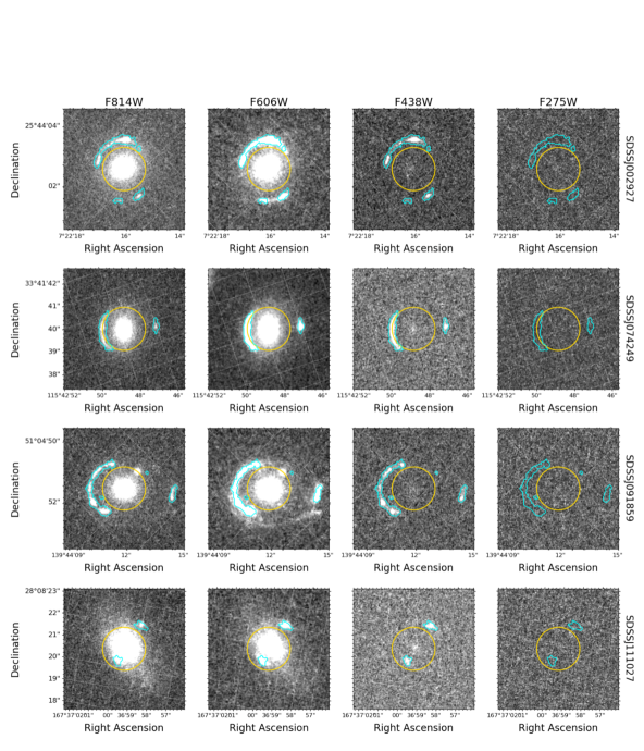
Figure 1: Lensed galaxies and extracted arc features. From left to right, we show the F814W, F606W, F438W, and F275W filter images for four of out targets. The cyan regions are the source arc structures extracted from the F438W mosaic using the residual_features_extraction code. The yellow circles show the 1 arcsec radius BOSS fiber. The mosaics shown in the Figure are the drizzled output images from astrodrizzle. To infer the photometry, we subtract the foreground lens galaxy from the mosaics first.

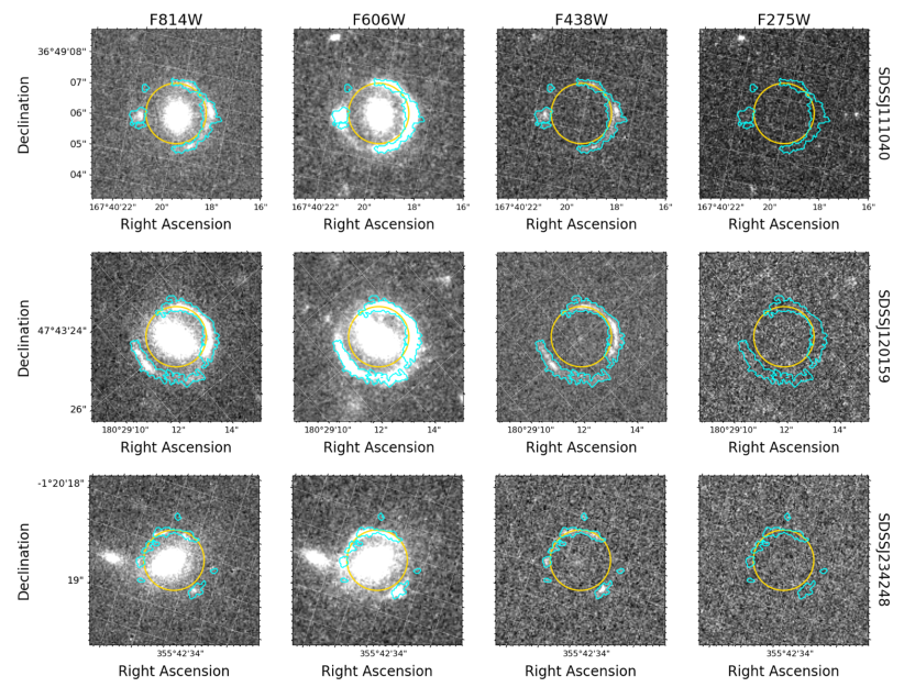
Figure 2: Same as Figure 1 for the three remaining targets of our sample. From left to right, we show the F814W, F606W, F438W, and the LyC filter (F275W for SDSSJ111040, and F225W for SDSSJ120159 and SDSSJ23248).

4 Data analysis

4.1 Estimation of the magnification factors

The first step of our analysis involves quantifying the magnification factors $\mu$ of our gravitationally lensed targets. We carry out our own lensing model to obtain the magnification factor $\mu$ for each one of the seven galaxies. Section A of the Appendix describe our modeling in details, while Table 4 lists the derived magnification factors. In the following, we adopt the more conservative values $\mu_{\rm a}$.

Table 4: Redshifts and magnification factors of the seven BELLS gallery analyzed in this work.

Target	$z_{lens}~{}^{a}$	$z_{Ly\alpha}~{}^{b}$	$z_{\rm sys}~{}^{c}$	$\mu_{\rm S}~{}^{d}$	$\mu_{\rm a}~{}^{e}$	$\mu_{\rm b}~{}^{f}$
SDSSJ002927	0.5869	2.4504	2.4500	14	12 $\pm$ 5	19 $\pm$ 7
SDSSJ074249	0.4936	2.3633	2.3625	16	17 $\pm$ 5	22 $\pm$ 7
SDSSJ091859	0.5811	2.4030	2.4000	18	11 $\pm$ 4	13 $\pm$ 5
SDSSJ111027	0.6073	2.3999	-	8	5 $\pm$ 3	7 $\pm$ 4
SDSSJ111040	0.7330	2.5024	-	17	11 $\pm$ 3	13 $\pm$ 3
SDSSJ120159	0.5628	2.1258	-	12	8 $\pm$ 3	14 $\pm$ 8
SDSSJ234248	0.5270	2.2649	-	23	7 $\pm$ 3	11 $\pm$ 4

4.2 Sérsic Fitting of the lens foreground ellipticals

The second step of the analysis involves quantifying the flux of the lensed galaxies in the observed filters F275W (F225W), F438W, F606W, and F814W. To accomplish this task, we need to eliminate any low-surface brightness flux emitted by the elliptical lens that might be contaminating the light from the background source. Therefore, we fit each foreground lens (in various wavelength bands) with a PSF-convolved 2D Sérsic model using the GALFIT software (Peng et al., 2002), and then we subtract its contribution from our images. To derive the Sérsic parameters of the foreground lens galaxies, we follow standard procedures employed by many previous studies (e.g., van der Wel et al., 2014). For each galaxy, we start with the F814W image, since it has the highest S/N ratio of all the filters. We perform source extraction of this image using SEP (Barbary et al., 2016) to estimate the gross properties of the lens galaxy, such as apparent magnitude, semi-minor and major axes lengths, and positional angle. By masking all the sources identified in this step, we compute the “background” contribution as the mean of the pixel-value distribution in the source masked image. Using these values as initial guesses, we fit the lens galaxy letting all the seven parameters of the Sérsic model to vary freely, except for the background value, which is left fixed (the background is estimated as described in the following subsection 4.4). To self-consistently obtain Sérsic models across the remaining wavelength bands, we rescale the best-fit, PSF-convolved F814W Sérsic model’s magnitude to the magnitudes of the F606W, F438W, and F275W (F225W) filters. These magnitudes are obtained by integrating the flux over a circular aperture of radius $\rm r=5\times$ the FWHM of the PSF within those bands. Finally, for each filter, we create residual images by subtracting the best-fit Sérsic model from the original images. We use these residual images to extract the arc structures of the lensed galaxies and quantify their properties, as explained in the next subsection 4.3.

4.3 Extraction of the Arcs

The second step of our analysis consists in establishing the aperture that encompasses the arc structures of our lensed targets. In order to do this, we employ the publicly available residual feature extraction software (Mantha et al., 2019). This pipeline is designed to work directly with the outputs of GALFIT, and works towards extracting both flux and area-wise significant contiguous regions of interest within the residual images. This software has proven to be efficient in extracting extended, low-surface brightness signatures within parametric model-subtracted images and has been demonstrated on HST imaging, notably also extracting gravitational arc structures (see Figure 10 in Mantha et al., 2019). One of the primary outputs of the feature extraction method is a binary segmentation map, where the extracted pixels that meet the criteria are labelled as 1 and all else as zero. These segmentation maps, corresponding to the extracted arc structures, serve as custom apertures for downstream photometry estimations.

We apply the Mantha et al. (2019) method to the residual images in the F438W filter. Since the foreground lens is intrinsically fainter in this band, with this choice we are minimizing any potential residual contribution (if any) from the lens. Once the segmentation map is derived for the F438W residual image, we apply it to the other bands. In Figures 1 and 2, we illustrate the extracted arc features (cyan contours) overlaid on top of the multiple wavelength images.

Table 5: Photometry of the lensed galaxies analyzed in this work.

Target	z	$\mu_{a}$	Area$~{}^{a}$	Filter	$\rm m_{AB}~{}^{b}$	$\rm M_{AB}~{}^{c}$	mLim
				F814W	22.43 $\pm$ 0.03	-20.06${}^{\pm 0.03}_{\pm 0.50}$	27.17
				F606W	22.28 $\pm$ 0.01	-20.21${}^{\pm 0.01}_{\pm 0.50}$	28.38
SDSSJ002927	2.45	12 $\pm$ 5	0.14	F438W	22.19 $\pm$ 0.02	-20.30${}^{\pm 0.02}_{\pm 0.50}$	27.13
				F275W	$\gtrsim$ 28.44	-	28.44
				F814W	22.41 $\pm$ 0.03	-19.63${}^{\pm 0.03}_{\pm 0.32}$	27.17
				F606W	22.35 $\pm$ 0.01	-19.69${}^{\pm 0.01}_{\pm 0.32}$	28.64
SDSSJ074249	2.36	17 $\pm$ 5	0.07	F438W	22.18 $\pm$ 0.03	-19.86${}^{\pm 0.03}_{\pm 0.32}$	26.95
				F275W	$\gtrsim$ 28.20	-	28.20
				F814W	21.77 $\pm$ 0.02	-20.78${}^{\pm 0.02}_{\pm 0.40}$	27.17
				F606W	21.49 $\pm$ 0.01	-21.06${}^{\pm 0.01}_{\pm 0.40}$	28.57
SDSSJ091859	2.40	11 $\pm$ 4	0.12	F438W	21.31 $\pm$ 0.02	-21.24${}^{\pm 0.02}_{\pm 0.40}$	26.95
				F275W	$\gtrsim$ 28.30	-	28.30
				F814W	24.33 $\pm$ 0.04	-19.07${}^{\pm 0.04}_{\pm 0.70}$	28.49
				F606W	24.27 $\pm$ 0.02	-19.14${}^{\pm 0.02}_{\pm 0.70}$	29.27
SDSSJ111027	2.40	5 $\pm$ 3	0.07	F438W	24.05 $\pm$ 0.04	-19.36${}^{\pm 0.04}_{\pm 0.70}$	28.38
				F275W	$\gtrsim$ 29.45	-	29.46
				F814W	22.31 $\pm$ 0.02	-20.31${}^{\pm 0.02}_{\pm 0.30}$	26.80
				F606W	22.20 $\pm$ 0.01	-20.42${}^{\pm 0.01}_{\pm 0.30}$	28.05
SDSSJ111040	2.50	11 $\pm$ 3	0.12	F438W	22.24 $\pm$ 0.02	-20.39${}^{\pm 0.02}_{\pm 0.30}$	26.73
				F275W	$\gtrsim$ 28.25	-	28.25
				F814W	21.65 $\pm$ 0.04	-21.02${}^{\pm 0.04}_{\pm 0.40}$	25.98
				F606W	21.53 $\pm$ 0.03	-21.14${}^{\pm 0.03}_{\pm 0.40}$	27.25
SDSSJ120159	2.13	8 $\pm$ 3	0.75	F438W	21.39 $\pm$ 0.03	-21.27${}^{\pm 0.03}_{\pm 0.40}$	26.28
				F225W	$\gtrsim$ 27.83	-	27.83
				F814W	23.70 $\pm$ 0.05	-19.23${}^{\pm 0.05}_{\pm 0.50}$	27.24
				F606W	23.53 $\pm$ 0.01	-19.40${}^{\pm 0.01}_{\pm 0.50}$	28.62
SDSSJ234248	2.27	7 $\pm$ 3	0.12	F438W	23.17 $\pm$ 0.03	-19.76${}^{\pm 0.03}_{\pm 0.50}$	27.27
				F225W	$\gtrsim$ 28.45	-	28.46

Table 6: $\beta$ slopes and color excesses $E(B-V)_{\rm fit}$ for our targets.

Target	$\beta$ slope a	$E(B-V)_{\rm fit}~{}^{b}$
SDSSJ002927	-2.35 $\pm$ 0.05	0.08 $\pm$ 0.01
SDSSJ074249	-2.00 $\pm$ 0.04	0.04 $\pm$ 0.02
SDSSJ091859	-2.28 $\pm$ 0.03	0.16 $\pm$ 0.01
SDSSJ111027	-2.05 $\pm$ 0.10	0.03 $\pm$ 0.02
SDSSJ111040	-2.21 $\pm$ 0.06	0.03 $\pm$ 0.02
SDSSJ120159	-2.02 $\pm$ 0.07	0.06 $\pm$ 0.04
SDSSJ234248	-2.42 $\pm$ 0.13	0.01 $\pm$ 0.01

4.4 Flux measurements

The fluxes and magnitudes of the lensed targets in the various bands are derived by summing the pixel fluxes within the segmentation map of the arc structures obtained in subsection 4.3. We observe that the light captured by our apertures in the LyC images (F225W or F275W) does not display emission above the noise threshold (see Figures 1 and 2). Nevertheless, it is possible that the presence of small, leaking knots could still hold significance if observed through a smaller aperture targeting a specific clump. Upon thorough examination of our images to investigate this possibility, we have conclusively ruled out the existence of any such small knots.

In order to derive upper limits on the LyC emission, we estimate the background level by dropping $1000$ random, identical circular apertures onto the original F275W and F225W filters images and measuring the background flux in each of them. The apertures are placed exclusively in regions that are free from contamination by background sources, and have the same area as the total number of pixels within the segmentation maps defined from the F438W residual images. The $1\sigma$ upper limits on the LyC emission are defined as the standard deviation of the background flux distribution. Table 5 summarizes the photometry of our targets in the available bands. Note that our magnitudes are corrected for galactic extinction using a Cardelli et al. (1989) extinction curve with $R_{V}=2.1$.

4.5 SED fitting and $\beta$ slope

We fit the observed photometry using the code Prospector (Johnson et al., 2021), in order to derive useful properties for the calculation of the LyC escape fractions (e.g., dust attenuation and intrinsic ratio between ionizing and non-ionizing continuum). We perform the fits assuming a non-parametric star formation history (SFH), defined on eight independent temporal bins ($>5$ bins is needed to recover more SFH details, Leja et al., 2019). The most recent bin spans $0-10$ Myrs in lookback time, and the remaining four bins are evenly spaced in $\rm log(lookback-time)$ up to $z=20$. Dust attenuation and stellar metallicity are allowed to vary as free parameters, while the redshift is kept constant. We explore the parameter space with DYNESTY (Speagle, 2020), a dynamic nested sampling method within Prospector. We adopt the Binary Population and Spectral Synthesis (BPASS, Eldridge et al. 2017) v2.2 stellar population models (using Simple Stellar Populations which include binary stars), and assume a Chabrier (2003a) initial mass function. Table 6 summarizes the color excesses $E(B-V)_{\rm fit}$ obtained from the fit assuming a Calzetti et al. (2000) attenuation curve.

Additionally, we use the observed photometry in the F606W and F814W filters to calculate the UV continuum slope $\beta$ of our targets. The error on the slopes is determined as the standard deviation of 100 measurements of $\beta$, obtained by varying the observed magnitudes within their errors. The derived $\beta$ values are listed in Table 6.

4.6 Lyman Continuum escape fraction

We use the following equation to derive upper limits on the relative escape fraction in our targets:

$$f_{esc}^{rel}=\frac{L(1500)/L(800)_{\rm int}}{f(1500)/f(800)_{\rm lim}}\times e^{\tau_{\rm IGM}}~{}~{}.$$ (1)

We assume $e^{\tau_{\rm IGM}}=1.72$, which is appropriate for $z\sim 2.3$ (see Haardt & Madau, 2012; Rutkowski et al., 2017). $f(1500)/f(800)_{\rm lim}$ is the observed ratio between the luminosity at 1,500 $\mathrm{\SIUnitSymbolAngstrom}$ and 800 $\mathrm{\SIUnitSymbolAngstrom}$, measured from the F606W and F275W (F225W) fluxes. $L(1500)/L(800)_{\rm int}$ is instead the ratio between the intrinsic luminosity at 1,500 $\mathrm{\SIUnitSymbolAngstrom}$ and 800 $\mathrm{\SIUnitSymbolAngstrom}$. Star-forming galaxies are typically modeled assuming $L(1500)/L(800)_{\rm int}=3$ (Steidel et al., 2001; Shapley et al., 2006; Grazian et al., 2016), which holds for luminosity densities given in units of $\rm erg\,s^{-1}\,Hz^{-1}$. Here, we derive the intrinsic ratio from the Prospector fits. For each galaxy, we first measure the mean fluxes of the best fit model around 800 $\mathrm{\SIUnitSymbolAngstrom}$ and 1,500 $\mathrm{\SIUnitSymbolAngstrom}$, and then we correct them for dust extinction assuming a Calzetti et al. (2000) attenuation curve and $E(B-V)_{\rm fit}$.

From $f_{esc}^{rel}$, we derive the absolute escape fractions as $f_{esc}^{abs}$ = $f_{esc}^{rel}$ $\times 10^{-0.4\,A_{1500}}$, where $A_{1500}$ is the dust attenuation at 1,500 Å. $A_{1500}$ is computed from $E(B-V)_{\rm fit}$, assuming a Calzetti et al. (2000) attenuation curve. The intrinsic $L(1500)/L(800)_{\rm int}$ and the upper limits on $f_{esc}^{rel}$ and $f_{esc}^{abs}$ are listed in Table 7.

Table 7: 1$\sigma$ upper limits on the relative and absolute escape fractions derived from the F275W(F225W) and the F606W data.

Target	$\mathit{\frac{L(\rm 1500)}{L(\rm 800)}}_{\rm int}^{~{}a}$	$f_{esc}^{rel}$	$f_{esc}^{abs}~{}^{b}$
SDSSJ002927	5.72	0.03378	0.01641
SDSSJ074249	3.98	0.03137	0.02208
SDSSJ091859	9.61	0.03107	0.00693
SDSSJ111027	3.52	0.05116	0.03944
SDSSJ111040	3.66	0.02409	0.01800
SDSSJ120159	2.99	0.01553	0.00857
SDSSJ234248	3.22	0.06295	0.05921

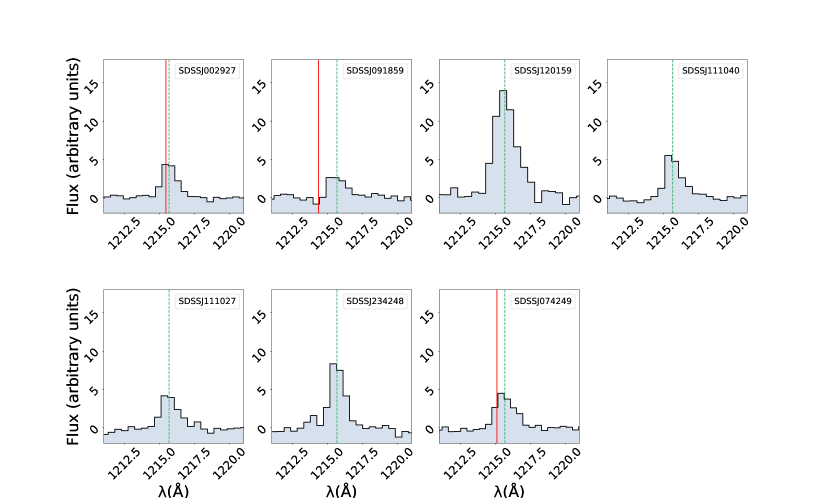
Figure 3: Ly$\alpha$ line profiles in wavelength space. The dotted green line marks the rest-frame wavelength 1215.67 $\mathrm{\SIUnitSymbolAngstrom}$. The red vertical lines marks the wavelength corresponding to $\Delta(v_{Ly\alpha})$ for the three galaxies for which the systemic redshift has been estimated. The y-axis is in arbitrary unit since the original spectrum is normalized by the starlight code.

4.7 $Ly\alpha$ properties

We measure the Ly$\alpha$ flux and equivalent width of the Ly$\alpha$ emission ($W_{Ly\alpha}$, hereafter) from the spectra and images. The continuum of the foreground elliptical galaxy is estimated by fitting the lens subtracted BOSS spectrum using the starlight full spectrum fitting code (Cid Fernandes et al., 2005). We use Bruzual & Charlot (2003) simple stellar population models, adopting a Chabrier IMF (Chabrier, 2003b), a grid of stellar metallicities Z = 0.0001, 0.0004, 0.004, 0.008, 0.02, 0.05, and ages from 10 Myrs to 3 Gyrs (i.e., the age of the Universe at $z\sim 2.3$). After subtracting the continuum from the BOSS spectrum, the Ly$\alpha$ fluxes are measured by direct integration of the Ly$\alpha$ profiles between $\sim$ 1,210 $\mathrm{\SIUnitSymbolAngstrom}$ and $\sim$ 1,220 $\mathrm{\SIUnitSymbolAngstrom}$. We use a Monte Carlo approach in order to infer the uncertainties on the flux measurements.

Figure 3 shows the Ly$\alpha$ line profiles of our targets. All the galaxies exhibit a prominent Ly$\alpha$ emission peak, with SDSSJ234248 possibly showing a red and a faint blue peak. We highlight that the observed Ly$\alpha$ emission is the one captured within the 2 arcsecond diameter BOSS fiber, which does not, or barely, include the arc structures (see Figures 1 and 2). Therefore, the observed Ly$\alpha$ emission is not indicative of the total emission within the lensed sources.

The FWHMs of the Ly$\alpha$ emission range between $250$ and $\sim 400\,\rm km\,s^{-1}$ (corrected for instrumental resolution). It is worth noticing that, for SDSSJ07429 and SDSSJ091859, Marques-Chaves et al. (2020) derived similar FWHMs from low-ionization ISM absorption lines (i.e., Si ii $\lambda$1260, Si ii $\lambda$1526 and C ii $\lambda$1334) within slits positioned on portions of the arc structures. Among the seven targets, we have systemic redshift ($z_{sys}$) estimates for SDSSJ07429, SDSSJ091859, and SDSSJ002927. For SDSSJ07429 and SDSSJ091859, $z_{sys}$ was derived from absorption, nebular and fine-structure emission lines (Marques-Chaves et al., 2020). For SDSSJ002927, we derive $z_{sys}$ from IR spectra observed with the LUCI instrument on the LBT telescope, using strong emission lines ($H\beta$, [O iii]$\lambda 4959$ and [O iii]$\lambda 5007$) (Citro et al. in prep). The velocity shifts with respect to systemic range between $\approx 60$ to 300 $\rm km\,s^{-1}$, and are reported in Table 8. According to Verhamme et al. (2015), velocity shifts smaller than $\approx 150$ km s^-1 are compatible with an optically thin ISM, with $\rm N_{HI}\sim 10^{17-17.5}\,cm^{-2}$.

From the Ly$\alpha$ fluxes, we compute the observed rest-frame Ly$\alpha$ equivalent width as:

$$\ W_{Ly\alpha}^{RF}=\frac{\rm Flux_{Ly\alpha}}{\rm F606W}\cdot\frac{1}{(1+z)}~{}~{},$$ (2)

where the F606W flux density is used as a proxy of the continuum at 1,216 $\mathrm{\SIUnitSymbolAngstrom}$, and $z$ is the redshift of our galaxies (where possible, we assume $z_{sys}$, otherwhise we use the redshift derived from the Ly$\alpha$ emission, $z_{Ly\alpha}$ - see Table 4). As already mentioned, since the Ly$\alpha$ is measured within the BOSS spectroscopic aperture, it is likely a lower limit to the total Ly$\alpha$ flux of each object. Accordingly, in the following Figures and Discussion, we consider these equivalent widths as lower limits.

Table 8: Properties of the Ly$\alpha$ emission line for the seven BELLS GALLERY galaxies analyzed in this work.

Target	$F_{Ly\alpha,obs}^{~{}a}$	$W_{Ly\alpha}^{RF}$b	$\Delta(v_{Ly\alpha})^{~{}c}$
SDSSJ002927	24.27 $\pm$ 0.97	19.59 $\pm$ 0.78	58.16 $\pm$ 0.48
SDSSJ074249	22.07 $\pm$ 0.52	21.36 $\pm$ 0.50	138.42 $\pm$ 0.3
SDSSJ091859	16.20 $\pm$ 0.46	8.84 $\pm$ 0.25	323.8 $\pm$ 2.04
SDSSJ111027	18.55 $\pm$ 3.15	98.51 $\pm$ 16.73	-
SDSSJ111040	29.16 $\pm$ 1.54	22.25 $\pm$ 1.18	-
SDSSJ120159	96.46 $\pm$ 0.92	52.26 $\pm$ 0.50	-
SDSSJ234248	41.26 $\pm$ 0.98	108.30 $\pm$ 2.58	-

5 Results and Discussion

5.1 Escape fraction vs. galaxy properties

In this subsection, we explore the relationships between the LyC escape fraction of our targets and their $\beta$ slope, $M_{UV}$ (from the F606W images), $W_{Ly\alpha}^{RF}$, and Ly$\alpha$ escape fraction.

In subsection 4.6, we derived that our targets are not LyC emitters, with LyC escape fractions $f_{esc}^{abs}$$\lesssim 6.5\%$ at 1$\sigma$ significance. Moreover, our findings of subsection 4.5 indicate that our targets have $\beta$ ranging between $-2.5$ and $-1.9$, and are consequently relatively low in dust content. Our median value of $\beta$ aligns with findings from other studies on faint galaxies (e.g., Venemans et al., 2005; Nilsson et al., 2007; Ouchi et al., 2008; Hayes et al., 2010; Ono et al., 2010; Nakajima et al., 2012; Matthee et al., 2016). The low dust content implied by the blue $\beta$ slopes are confirmed by the Prospector fits to the photometry, which indicate $E(B-V)_{\rm fit}$ ranging between 0.01 to 0.16 (see Table 6).

Figure 4 shows the comparison between the distribution of the $\beta$ slopes of our targets and that of the low-redshift LzLCS+ sample (i.e., LzLCS galaxies from Flury et al., 2022a, b combined with HST/COS data from Izotov et al., 2016a, b, 2018a, 2018b; Wang et al., 2019 and Izotov et al., 2021). It is evident that our galaxies show $\beta$ values that overlap with the LzLCS+ distribution. However, at $\beta\lesssim-2$, the majority of the local galaxies are characterized by $f_{esc}^{abs}$ $>10\%$ at 1$\sigma$ significance. For similar $\beta$, our galaxies show instead $f_{esc}^{abs}$ $\lesssim 6.5\%$ at 1$\sigma$ significance. Our results are similar to what observed by Jung et al. (2024) in galaxies with $-18\lesssim M_{UV}\lesssim-21$ at $z\sim 1.3-3$.

Figure 4: $\beta$ frequency distribution for our targets and LzLCS+ targets (i.e., LzLCS galaxies from Flury et al., 2022a, b combined with HST/COS data from Izotov et al., 2016a, b, 2018a, 2018b; Wang et al., 2019).The silver histogram represents the $\beta$ distribution for local galaxies with $f_{esc}^{abs}$ $>10\%$ at 1$\sigma$ significance. The black histogram shows the distribution for local galaxies with $f_{esc}^{abs}$ $<10\%$ at 1$\sigma$ significance. The red histogram illustrates the $\beta$ distribution for our sample ($f_{esc}^{abs}$ $\lesssim 6.5\%$ at 1$\sigma$ significance).

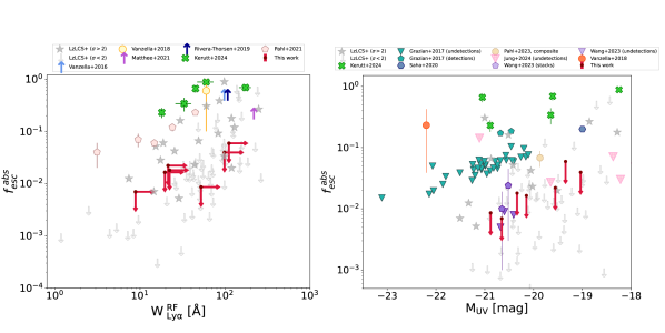
Figure 5: Left panel: $f_{esc}^{abs}$vs. $W_{Ly\alpha}$ plane. Black and grey symbols are measurements in the local Universe at different detection levels (stars - $>2\sigma$, downward pointing arrows $<2\sigma$) from the LzLCS+ sample. High redshift LyC leakers are marked with colored symbols. Specifically, we show Ion2 (Vanzella et al., 2016), Ion3 (Vanzella et al., 2018), the Sunburst Arc (Rivera-Thorsen et al., 2019), GS 30668/XLS-26 (Naidu et al., 2017; Matthee et al., 2021). We also show results from Pahl et al. (2021) and Kerutt et al. (2024). Red downward and rightward pointing arrows are the $1\sigma$ $f_{esc}^{abs}$ upper limits and the lower limits on the $W_{Ly\alpha}^{RF}$ for the seven BELLS GALLERY galaxies studied in this work. Right panel: absolute escape fractions as a function of the UV magnitude at 1,500 $\mathrm{\SIUnitSymbolAngstrom}$. Black and grey symbols are color coded as in the left panel. Red downward pointing arrows are the $1\sigma$ $f_{esc}^{abs}$ upper limits for the seven BELLS GALLERY galaxies studied in this work. Downward pointing triangles of different colors are undetections from Grazian et al. (2016) (1$\sigma$), Wang et al. (2023) (2$\sigma$), and Jung et al. (2024) (1$\sigma$). Other symbols are detections from Grazian et al. (2016), Wang et al. (2023), Vanzella et al. (2018), Saha et al. (2020), Pahl et al. (2023), and Kerutt et al. (2024), respectively (when relative escape fractions are provided, we transform them into absolute escape fractions by multiplying assuming a Calzetti et al. (2000) attenuation curve and $\rm E(B-V)=0.1$).

Figure 5 shows $f_{esc}^{abs}$ as a function of $W_{Ly\alpha}$ (left panel) and $M_{UV}$ (right panel) for our galaxies and compiled literature data at various redshifts. Studies in the local Universe (grey symbols in the Figures) extend the measurements to faint UV magnitudes and escape fraction measurements/limits down to sub-percent values. Conversely, high redshift studies are typically limited to larger values of the escape fraction (e.g., Grazian et al., 2016; Vanzella et al., 2016; Jung et al., 2024; Kerutt et al., 2024). Our sample is able to set a very stringent upper limit on the escape fraction of LyC radiation down to $M_{UV}=-19$ at $z\sim 2$.

Figure 5 (left panel) shows the relation between $f_{esc}^{abs}$ and $W_{Ly\alpha}^{RF}$ for the galaxies analyzed in this work, compared to data at different redshifts. The $W_{Ly\alpha}^{RF}$ of the BELLS GALLERY galaxies range from $\sim$ 10 to $\sim$ 100 $\mathrm{\SIUnitSymbolAngstrom}$, similar to the values observed in the local LzLCS+ sample. In this range, most of the LzLCS+ galaxies are not LyC leakers, which would be consistent with the observed non detections. However, as mentioned earlier, the $W_{Ly\alpha}$ of our $z\sim 2$ galaxies should be considered as lower limits. Given what is known about the extent of Ly$\alpha$ emission in both local and high redshift galaxies (e.g., Hayes et al., 2013; Leclercq et al., 2017; Erb et al., 2018; Claeyssens et al., 2022; Erb et al., 2023), it is entirely plausible that the Ly$\alpha$ emission within the BOSS fiber is largely underestimating the real emission. To quantify this effect, we estimate the total Ly$\alpha$ flux using relations based on low redshift galaxies. Specifically, we estimate the total Ly$\alpha$ flux by multiplying the $W_{Ly\alpha}^{prod}$ derived from the Prospector fits by the UV continuum in the F606W band. We then assume that this flux is distributed in 9 $\times$ area of the UV continuum (following Hayes et al., 2013). From this calculation, we derive that the BOSS fiber contains only up to $\sim 40$ % of the actual emission, bringing the actual $W_{Ly\alpha}$ range to $\sim$ 15 - 200 $\mathrm{\SIUnitSymbolAngstrom}$. At $W_{Ly\alpha}$$\sim 100$ $\mathrm{\SIUnitSymbolAngstrom}$, we would expect more than 50 % of the galaxies to be LyC emitters, based on the results by Flury et al. (2022b).

5.2 An analytical approach to model the LyC and $Ly\alpha$ radiative transfer

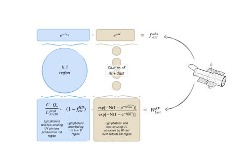
Figure 6: Schematic view of our models and $W_{Ly\alpha}^{RF}$ parameterization in the case of a dust screen positioned ahead of an H II region, the source of Ly$\alpha$ photons. It is important to highlight that the observed escape fraction $f_{esc}^{abs}$  consistently remains lower than the escape fraction at the outer edge of the H II region ($f_{~{}esc}^{~{}H\,II}$), as LyC photons can be absorbed by the neutral hydrogen and dust within the clumpy dust screen.

In this subsection, we develop a simple toy-model to describe the effects of radiative transfer of Ly$\alpha$ and non-ionizing UV photons on the resulting rest-frame $W_{Ly\alpha}^{RF}$. We assume that young stars produce a spherical H ii region, free of dust, where Ly$\alpha$ is produced after recombination. The star light and the Ly$\alpha$ photons then travel through a clumpy screen of dust and H i. In this model, schematically shown in Figure 6, the observed $W_{Ly\alpha}^{RF}$ depends on the value of the equivalent width of the Ly$\alpha$ at the outer edge of the H ii region ($W_{Ly\alpha}^{H\,II}$) and on the radiative transport of Ly$\alpha$ and continuum photons through the clumpy medium. $W_{Ly\alpha}^{H\,II}$ depends on the intrinsic $W_{Ly\alpha}^{prod}$ (i.e., resulting from age, metallicity and IMF-dependent stellar population – assuming all ionizing photons are absorbed), and on the fraction of ionizing photons that are absorbed by H i in the H ii region. Accordingly:

$$W_{Ly\alpha}^{H\,II}=W_{Ly\alpha}^{prod}\cdot(1-f_{esc}^{H\,II})=\frac{C\cdot Q_{0}}{L_{\lambda 1216}^{prod}}(1-f_{esc}^{H\,II}),$$ (3)

where $Q_{0}$ is the number of ionizing photons, $C=1.04\times 10^{-11}$ erg is the Ly$\alpha$ emission coefficient for Case B recombination, $n_{e}=100$ cm^-3 (see Schaerer, 2003), $L_{\lambda 1216}^{prod}$ is the continuum luminosity at 1,216 $\mathrm{\SIUnitSymbolAngstrom}$, and $(1-f_{esc}^{H\,II})$ is the fraction of LyC photons absorbed in the H II region and resulting in Ly$\alpha$. Note that $f_{esc}^{H\,II}$ is not the global LyC escape fraction measured at Earth, as ionizing photons that are not used to produce nebular lines still need to traverse the galaxy’s ISM/CGM, where they can be absorbed by dust and neutral hydrogen.

According to the chosen geometry, the attenuation due to the clumps can be written as $exp[{-N(1-e^{-(\tau_{ISM,c}^{\lambda 912}+\tau_{HI,c})})]}$, where $N$ is the average number of clumps along the line of sight (e.g., Scarlata et al., 2009). Given that $(\tau_{ISM}^{\lambda 912}+\tau_{HI})>>1$, (with $\tau_{ISM}^{\lambda 912}<<\tau_{HI}$), this expression can be approximated as $e^{-N}$, i.e., the covering fraction of the clumps. Ly$\alpha$ photons are not destroyed when absorbed by H i, but rather re-emitted along different directions and with a frequency shift that depends on the gas motions, resulting in an excess probability (with respect to non-resonant photons) of being absorbed by dust. This effect can be modeled using the “scattering $q-$parameter” introduced by Scarlata et al. (2009) and Finkelstein et al. (2009). The resulting attenuation of Ly$\alpha$ photons is $exp[-N(1-e^{-q\tau_{ISM}^{\lambda 1216}})]$.

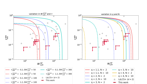
Figure 7: Toy model curves overimposed to the LzLCS+ ($\sigma>2$) (grey stars) and our seven targets (red arrows, 1$\sigma$ significance). Left panel: models vary in $\tau_{~{}ISM}^{~{}\lambda 1216}$ and $W_{Ly\alpha}^{prod}$ according to the colors and line styles described in the legend. Values of $q=2$ and $N=3$ are assumed. Right panel: models vary in $q$ and $N$ according to the colors and line styles described in the legend. Values of $W_{Ly\alpha}^{prod}$ = 200 $\mathrm{\SIUnitSymbolAngstrom}$ and $\tau_{~{}ISM}^{~{}\lambda 1216}$= 0.2 are assumed.

To summarize, $W_{Ly\alpha}^{RF}$ can be written as:

$$W_{Ly\alpha}^{RF}=W_{Ly\alpha}^{prod}\cdot(1-f_{esc}^{H\,II})\cdot\frac{exp[-N(1-e^{-q\tau_{ISM}^{\lambda 1216}})]}{exp[-N(1-e^{-\tau_{ISM}^{\lambda 1216}})]},$$ (4)

where $\rm\tau_{ISM}^{\lambda 1216}$ is the dust optical depth at 1,216 $\mathrm{\SIUnitSymbolAngstrom}$.

Figure 7 shows the analytical models overimposed to our data and the LzLCS+ results with $>2\sigma$ significance. We observe that an increase in $\tau_{~{}ISM}^{~{}\lambda 1216}$ leads to a decrease of both $f_{esc}^{abs}$ and $W_{Ly\alpha}^{RF}$. Additionally, decreasing $W_{Ly\alpha}^{prod}$, increasing the number of clumps $N$, or increasing the scattering parameter $q$ leads to a decrease in $W_{Ly\alpha}^{RF}$. The LzLCS+ galaxies with higher $f_{esc}^{abs}$ can be modeled with a low $\tau_{~{}ISM}^{~{}\lambda 1216}$, a high $W_{Ly\alpha}^{prod}$, a low $q$, and a low $N$. It is interesting to note that the parameters required to reproduce the LzLCS+ galaxy with $f_{esc}^{abs}$$\sim 90\%$ are particularly extreme, involving either an $W_{Ly\alpha}^{prod}$$>1000$ $\mathrm{\SIUnitSymbolAngstrom}$, a $\tau_{~{}ISM}^{~{}\lambda 1216}$$<0.05$, or nearly zero covering fractions. Instead, galaxies with lower $f_{esc}^{abs}$ and $W_{Ly\alpha}^{RF}$ are generally characterized by either a lower $W_{Ly\alpha}^{prod}$, a higher $q$, or a higher $N$. Unfortunately, our models are degenerate, with different combinations of the parameters producing similar values of $W_{Ly\alpha}^{RF}$ and $f_{esc}^{abs}$. Currently, we lack the necessary information to break this degeneracy. Independent measurements, such as the H$\alpha$ and H$\beta$ lines, could help determine the covering fraction of the clumps $e^{-N}$ (Scarlata et al., 2009) which, combined with the derived $\tau_{~{}ISM}^{~{}\lambda 1216}$, $f_{esc}^{abs}$, and $W_{Ly\alpha}^{prod}$, would allow us to estimate $q$ and understand the degree of scattering that Ly$\alpha$ photons experience on their way out of the galaxy.

5.3 $Ly\alpha$ escape fraction

Using the results from the SED fitting discussed in subsection 5.1, we can compute the escape fraction of Ly$\alpha$ radiation, that we define as $W_{Ly\alpha}^{RF}$/$W_{Ly\alpha}^{prod}$. Flury et al. (2022b) show that there is a strong correlation in the local universe between the Ly$\alpha$ and LyC escape fractions.

The Ly$\alpha$ and LyC escape fractions are compared in Figure 8. The $z\sim 2.5$ galaxies studied here have higher Ly$\alpha$ escape fractions than the low-$z$ galaxies’ distribution, result that is even stronger when considering that the observed Ly$\alpha$ fluxes are lower limits (see subsection 5.1). Given the strong correlation between the Ly$\alpha$ and LyC escape fractions in the local universe, the Ly$\alpha$ escape fraction is expected to be a reliable indicator of the the LyC escape fraction. How, then, can we reconcile this with the LyC non-detections and the strong upper limits suggested by our measurements?

We suggest that this discrepancy may be due to an increasing neutral gas fraction for higher redshift/lower mass galaxies (e.g., Chen et al., 2021; Papastergis et al., 2012; Maddox et al., 2015), accompanied by a progressively lower dust content (e.g., Cucciati et al., 2012; Hayes et al., 2011; Eales & Ward, 2024). This would follow naturally given that the dust-to-gas ratio is observed to decrease with both metallicity (e.g., Rémy-Ruyer et al., 2014) and stellar mass (e.g., Santini et al., 2014), a trend that seems to hold well into the reionization epoch (e.g., Heintz et al., 2024). At high redshifts, the increased amount of neutral hydrogen and the reduced dust attenuation result in a scenario where LyC radiation is entirely absorbed by neutral hydrogen, while Ly$\alpha$ radiation escapes thanks to the minimal dust content, despite enhanced scattering in neutral gas. This scenario could be tested via measurements of the Ly$\alpha$ line profiles, as radiative transfer models suggest that high column densities of H i produce broad Ly$\alpha$ profiles, with large shifts with respect to systemic. With only velocity shifts for three objects, we cannot explore this test at this point.

The proposed scenario may also be related to the “Low escape” phase proposed by Naidu et al. (2022), in which channels created by stellar feedback may be refilling with H i, making it difficult for LyC photons to escape while still allowing Ly$\alpha$ photons to do so, if the dust content is low. However, this evolutionary phase would be relatively short-lived (approximately $10-100$ Myrs), making it unlikely that all of our galaxies are currently experiencing it.

Ultimately, we cannot rule out that our findings are influenced by how BOSS captures the Ly$\alpha$ emission in the extended halo, whereas LyC emission is measured at the sites of continuum production. In fact, the observed Ly$\alpha$ emission might have undergone a different radiative transfer compared to the LyC emission. Spatially resolved maps of the Ly$\alpha$ emission are needed, alongside the existing LyC leakage maps, in order to confirm the true nature of these galaxies and test our hypotheses.

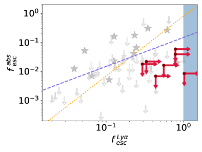
Figure 8: $f_{esc}^{abs}$ vs. $f_{esc}^{Ly\alpha}$. Symbols are color coded as in Figure 5. The purple dashed and orange dotted lines are the $f_{esc}^{abs}$ vs. $f_{esc}^{Ly\alpha}$ relations by Begley et al. (2024) (VANDELS galaxies) and Izotov et al. (2024) ($z<0.5$), respectively. The blue shaded area on the right marks the unphysical region of $f_{esc}^{Ly\alpha}$$>1$. Note that our galaxies have high $f_{esc}^{Ly\alpha}$lower limits ($\gtrsim 30\%$).

6 Conclusions

In this paper we investigate the relation between the LyC leakage and Ly$\alpha$ emission in a sample of seven $z\sim 2$ gravitationally lensed Ly$\alpha$ emitters drawn from the BELLS GALLERY Survey (Brownstein et al., 2012). Our galaxies have $-21\lesssim M_{UV}\lesssim-19$, and are dust poor (with $\beta$ ranging between $-1.9$ and $-2.4$). From the UV broad band F275W and F225W HST filters, we provide direct upper limit measurements of the emission below 912Å, from which we estimate upper limits on $f_{esc}^{abs}$. We also use the BOSS spectra to measure lower limits on the Ly$\alpha$ fluxes and Ly$\alpha$ equivalent widths. We create a simple analytical model to describe the connection between Ly$\alpha$ emission, LyC leakage, H I column density, dust, and scattering effects. We find that the seven BELLS GALLERY galaxies exhibit similar $\beta$ slopes as nearby galaxies. However, while local sources show $f_{esc}^{abs}$$\gtrsim 10$ at $1\sigma$ significance, our high redshift targets have $f_{esc}^{abs}$($1\sigma$) $\lesssim 6.5\%$ at 1$\sigma$ significance. Additionally, we find that the Ly$\alpha$ escape fraction of the BELLS galaxies is higher than for local galaxies for a given Ly$\alpha$ equivalent width.

We believe that our findings reflects the observed increase in neutral hydrogen and decrease in dust content in high-redshift galaxies: the combination of these factors reduces the escape fraction of LyC radiation, while still enabling Ly$\alpha$ emission to escape, despite the large number of scatterings. Our result implies that the LyC leaking mechanisms could work differently at high redshift, and therefore that using LyC low-redshift indirect estimators to interpret the high redshift Universe might be incorrect. However, additional independent data, such as spatially resolved Ly$\alpha$ imaging within the arc structures, high resolution Ly$\alpha$ profiles and optical stellar spectra are necessary to confirm our hypothesis.

Appendix A Lensing models

Shu et al. (2016b) presented lens models for the seven systems studied here. In order to obtain uncertainties on the sources magnifications we carry out our own modeling.

Our lens mass models are very similar to those of Shu et al. (2016b), but the lens reconstructions method is somewhat different. Multiple image lens reconstruction of extended sources, like LAEs, relies on the fact that surface brightness is preserved under lensing mapping from the source to the lens plane. First, from the original F814W HST images we remove all pixels with counts below 0.015/s, because most of these appear to be noise. The remaining pixels that are clearly not a part of the lensed images are also removed.

Our lens mass models consist of a single elliptical alphapot potential (Keeton, 2001) with a small core ($<0.1^{\prime\prime}$), $r_{c}$, centered at $(x_{0},y_{0})$. The corresponding density profile is a power law of slope $\alpha$. We also include an external shear, whose two parameters, $\gamma_{x}$ and $\gamma_{y}$ subsume the influence of outside mass as well as azimuthal complexities in the lens itself. The priors on the alphapot parameters are: the slope of the density profile was $\alpha\in[-0.85,1.15]$, position angle of the lens was limited to $\pm 10^{\circ}$ of the observed light PA, and the ellipticity of the potential to $b/a>0.8$, corresponding to the ellipticity of the mass distribution of $b/a>0.55$. The center of the lens was allowed to vary within 3 pixels, or $\pm 0.12^{\prime\prime}$ from the light center of the lensing galaxy.

We backproject lens plane pixels to the source plane, and optimize the parameters of the lens using downhill simplex for 9 free parameters: normalization of the potential, $\alpha$, $r_{c}$, $x_{0}$, $y_{0}$, $\gamma_{x}$, $\gamma_{y}$, PA, and $b/a$. Our figure of merit to be minimized is a product of two criteria, both defined in the source plane: (i) since the images that backproject to the same source plane location must arise from the same portion of the source, the rms of fluxes of overlapping backprojected pixels at any source plane location should be small, and (ii) the source plane area occupied by high surface brightness pixels in the lens plane should be small. The second criterion is similar to that used in point-image reconstruction, where point images would ideally converge to the same source plane location. In practice, this can lead to overfocusing and higher implied magnifications, however, in our case this is mitigated by the first criterion. Furthermore, because of the extended nature of the images and their uneven shape, and the restrictions imposed by what lensing deflection fields can do, overfocusing is unlikely to significantly affect magnification estimates.

While we optimize in the source plane only, we do check that the forward lensed images are in reasonable agreement with the observed images. We generate 100 models for each of the seven systems, and use these to derive uncertainties on source magnification. Our resulting reconstructed sources are non-parametric. Their shape and orientation are similar to those Shu et al. (2016b). The resulting density slopes of our models tend to be somewhat shallower than isothermal, extending to $\alpha\sim-0.9$.

We calculate two magnification values for each source: using 0.018 counts/s, and 0.025 counts/s as the lower limit on the flux. We chose these because at fluxes below 0.018 counts/s noise pixels begin to appear everywhere in the image, while above 0.025 counts/s most of the pixels belong to the lensed images. The former magnifications are lower than the latter because down to 0.018 counts/s, images (and sources) are more extended and so many regions of the source are far from caustics, i.e. lines in the source plane where magnifications are infinite for point sources. We note that magnification estimates depend on whether the source is assumed to be smooth or structured, for example, having very peaked central flux density. In our reconstructions the source plane grid resolution is 0.05 of the total extent of the backprojected pixels in each of the two orthogonal directions. If we assumed a grid $4\times$ finer in $x$ and $y$, our magnification values would be 10% - 50% larger. Our median magnification values, and the corresponding values from Shu et al. (2016b) are in Table 4. We highlight that the lensing magnification is not achromatic, as continuum and Ly$\alpha$ photons have different spatial distributions (the Ly$\alpha$ photons are certainly extended beyond the arc structures and within the BOSS aperture). Overcoming these problems requires angular resolution maps of the Ly$\alpha$ emission which we do not possess at this time.

References

- Alexandroff et al. (2015) Alexandroff, R. M., Heckman, T. M., Borthakur, S., Overzier, R., & Leitherer, C. 2015, ApJ, 810, 104, doi: 10.1088/0004-637X/810/2/104
- Barbary et al. (2016) Barbary, K., Boone, K., McCully, C., et al. 2016, kbarbary/sep: v1.0.0, v1.0.0, Zenodo, Zenodo, doi: 10.5281/zenodo.159035
- Begley et al. (2022) Begley, R., Cullen, F., McLure, R. J., et al. 2022, MNRAS, 513, 3510, doi: 10.1093/mnras/stac1067
- Begley et al. (2024) —. 2024, MNRAS, 527, 4040, doi: 10.1093/mnras/stad3417
- Bergvall et al. (2013) Bergvall, N., Leitet, E., Zackrisson, E., & Marquart, T. 2013, A&A, 554, A38, doi: 10.1051/0004-6361/201118433
- Bian et al. (2017) Bian, F., Fan, X., McGreer, I., Cai, Z., & Jiang, L. 2017, ApJ, 837, L12, doi: 10.3847/2041-8213/aa5ff7
- Bouwens et al. (2012) Bouwens, R. J., Illingworth, G. D., Oesch, P. A., et al. 2012, ApJ, 754, 83, doi: 10.1088/0004-637X/754/2/83
- Brownstein et al. (2012) Brownstein, J. R., Bolton, A. S., Schlegel, D. J., et al. 2012, ApJ, 744, 41, doi: 10.1088/0004-637X/744/1/41
- Bruzual & Charlot (2003) Bruzual, G., & Charlot, S. 2003, MNRAS, 344, 1000, doi: 10.1046/j.1365-8711.2003.06897.x
- Calzetti et al. (2000) Calzetti, D., Armus, L., Bohlin, R. C., et al. 2000, ApJ, 533, 682, doi: 10.1086/308692
- Cardelli et al. (1989) Cardelli, J. A., Clayton, G. C., & Mathis, J. S. 1989, ApJ, 345, 245, doi: 10.1086/167900
- Cen & Kimm (2015) Cen, R., & Kimm, T. 2015, ApJ, 801, L25, doi: 10.1088/2041-8205/801/2/L25
- Chabrier (2003a) Chabrier, G. 2003a, PASP, 115, 763, doi: 10.1086/376392
- Chabrier (2003b) —. 2003b, PASP, 115, 763, doi: 10.1086/376392
- Chen et al. (2021) Chen, Q., Meyer, M., Popping, A., et al. 2021, MNRAS, 508, 2758, doi: 10.1093/mnras/stab2810
- Chisholm et al. (2020) Chisholm, J., Prochaska, J. X., Schaerer, D., Gazagnes, S., & Henry, A. 2020, MNRAS, 498, 2554, doi: 10.1093/mnras/staa2470
- Chisholm et al. (2022) Chisholm, J., Saldana-Lopez, A., Flury, S., et al. 2022, MNRAS, 517, 5104, doi: 10.1093/mnras/stac2874
- Cid Fernandes et al. (2005) Cid Fernandes, R., Mateus, A., Sodré, L., Stasińska, G., & Gomes, J. M. 2005, MNRAS, 358, 363, doi: 10.1111/j.1365-2966.2005.08752.x
- Claeyssens et al. (2022) Claeyssens, A., Richard, J., Blaizot, J., et al. 2022, A&A, 666, A78, doi: 10.1051/0004-6361/202142320
- Cucciati et al. (2012) Cucciati, O., Tresse, L., Ilbert, O., et al. 2012, A&A, 539, A31, doi: 10.1051/0004-6361/201118010
- Eales & Ward (2024) Eales, S., & Ward, B. 2024, MNRAS, 529, 1130, doi: 10.1093/mnras/stae403
- Eldridge et al. (2017) Eldridge, J. J., Stanway, E. R., Xiao, L., et al. 2017, PASA, 34, e058, doi: 10.1017/pasa.2017.51
- Erb et al. (2023) Erb, D. K., Li, Z., Steidel, C. C., et al. 2023, ApJ, 953, 118, doi: 10.3847/1538-4357/acd849
- Erb et al. (2010) Erb, D. K., Pettini, M., Shapley, A. E., et al. 2010, ApJ, 719, 1168, doi: 10.1088/0004-637X/719/2/1168
- Erb et al. (2018) Erb, D. K., Steidel, C. C., & Chen, Y. 2018, ApJ, 862, L10, doi: 10.3847/2041-8213/aacff6
- Finkelstein et al. (2009) Finkelstein, S. L., Rhoads, J. E., Malhotra, S., & Grogin, N. 2009, ApJ, 691, 465, doi: 10.1088/0004-637X/691/1/465
- Fletcher et al. (2019) Fletcher, T. J., Tang, M., Robertson, B. E., et al. 2019, ApJ, 878, 87, doi: 10.3847/1538-4357/ab2045
- Flury et al. (2022a) Flury, S. R., Jaskot, A. E., Ferguson, H. C., et al. 2022a, ApJS, 260, 1, doi: 10.3847/1538-4365/ac5331
- Flury et al. (2022b) —. 2022b, ApJ, 930, 126, doi: 10.3847/1538-4357/ac61e4
- Gaia Collaboration et al. (2022) Gaia Collaboration, Vallenari, A., Brown, A. G. A., et al. 2022, arXiv e-prints, arXiv:2208.00211, doi: 10.48550/arXiv.2208.00211
- Gazagnes et al. (2020) Gazagnes, S., Chisholm, J., Schaerer, D., Verhamme, A., & Izotov, Y. 2020, A&A, 639, A85, doi: 10.1051/0004-6361/202038096
- Gazagnes et al. (2018) Gazagnes, S., Chisholm, J., Schaerer, D., et al. 2018, A&A, 616, A29, doi: 10.1051/0004-6361/201832759
- Gonzaga et al. (2012) Gonzaga, S., Hack, W., Fruchter, A., & Mack, J. 2012, The DrizzlePac Handbook (Baltimore, MD: STScI). {https://hst-docs.stsci.edu/drizzpac}
- Grazian et al. (2016) Grazian, A., Giallongo, E., Gerbasi, R., et al. 2016, A&A, 585, A48, doi: 10.1051/0004-6361/201526396
- Haardt & Madau (2012) Haardt, F., & Madau, P. 2012, ApJ, 746, 125, doi: 10.1088/0004-637X/746/2/125
- Hayes et al. (2011) Hayes, M., Schaerer, D., Östlin, G., et al. 2011, ApJ, 730, 8, doi: 10.1088/0004-637X/730/1/8
- Hayes et al. (2010) Hayes, M., Östlin, G., Schaerer, D., et al. 2010, Nature, 464, 562, doi: 10.1038/nature08881
- Hayes et al. (2013) —. 2013, ApJ, 765, L27, doi: 10.1088/2041-8205/765/2/L27
- Hayes et al. (2023) Hayes, M. J., Runnholm, A., Scarlata, C., Gronke, M., & Rivera-Thorsen, T. E. 2023, MNRAS, 520, 5903, doi: 10.1093/mnras/stad477
- Heckman et al. (2001) Heckman, T. M., Sembach, K. R., Meurer, G. R., et al. 2001, ApJ, 558, 56, doi: 10.1086/322475
- Heckman et al. (2011) Heckman, T. M., Borthakur, S., Overzier, R., et al. 2011, ApJ, 730, 5, doi: 10.1088/0004-637X/730/1/5
- Heintz et al. (2024) Heintz, K. E., Brammer, G. B., Watson, D., et al. 2024, arXiv e-prints, arXiv:2404.02211, doi: 10.48550/arXiv.2404.02211
- Henry et al. (2018) Henry, A., Berg, D. A., Scarlata, C., Verhamme, A., & Erb, D. 2018, ApJ, 855, 96, doi: 10.3847/1538-4357/aab099
- Henry et al. (2015) Henry, A., Scarlata, C., Martin, C. L., & Erb, D. 2015, ApJ, 809, 19, doi: 10.1088/0004-637X/809/1/19
- Hinshaw et al. (2013) Hinshaw, G., Larson, D., Komatsu, E., et al. 2013, ApJS, 208, 19, doi: 10.1088/0067-0049/208/2/19
- Hoffmann et al. (2021) Hoffmann, S. L., Mack, J., & Avila, R. J. 2021, The DrizzlePac Handbook, Version 2.0 (Baltimore, MD: STScI). {https://hst-docs.stsci.edu/drizzpac}
- Inoue et al. (2014) Inoue, A. K., Shimizu, I., Iwata, I., & Tanaka, M. 2014, MNRAS, 442, 1805, doi: 10.1093/mnras/stu936
- Izotov et al. (2016a) Izotov, Y. I., Orlitová, I., Schaerer, D., et al. 2016a, Nature, 529, 178, doi: 10.1038/nature16456
- Izotov et al. (2016b) Izotov, Y. I., Schaerer, D., Thuan, T. X., et al. 2016b, MNRAS, 461, 3683, doi: 10.1093/mnras/stw1205
- Izotov et al. (2018a) Izotov, Y. I., Schaerer, D., Worseck, G., et al. 2018a, MNRAS, 474, 4514, doi: 10.1093/mnras/stx3115
- Izotov et al. (2024) Izotov, Y. I., Thuan, T. X., Guseva, N. G., et al. 2024, MNRAS, 527, 281, doi: 10.1093/mnras/stad3151
- Izotov et al. (2021) Izotov, Y. I., Worseck, G., Schaerer, D., et al. 2021, MNRAS, 503, 1734, doi: 10.1093/mnras/stab612
- Izotov et al. (2018b) —. 2018b, MNRAS, 478, 4851, doi: 10.1093/mnras/sty1378
- Jaskot & Oey (2013) Jaskot, A. E., & Oey, M. S. 2013, ApJ, 766, 91, doi: 10.1088/0004-637X/766/2/91
- Johnson et al. (2021) Johnson, B. D., Leja, J., Conroy, C., & Speagle, J. S. 2021, ApJS, 254, 22, doi: 10.3847/1538-4365/abef67
- Jung et al. (2024) Jung, I., Ferguson, H. C., Hayes, M. J., et al. 2024, arXiv e-prints, arXiv:2403.02388, doi: 10.48550/arXiv.2403.02388
- Keeton (2001) Keeton, C. R. 2001, arXiv e-prints, astro. https://arxiv.org/abs/astro-ph/0102341
- Kerutt et al. (2024) Kerutt, J., Oesch, P. A., Wisotzki, L., et al. 2024, A&A, 684, A42, doi: 10.1051/0004-6361/202346656
- Kimm et al. (2022) Kimm, T., Bieri, R., Geen, S., et al. 2022, ApJS, 259, 21, doi: 10.3847/1538-4365/ac426d
- Kimm et al. (2019) Kimm, T., Blaizot, J., Garel, T., et al. 2019, MNRAS, 486, 2215, doi: 10.1093/mnras/stz989
- Leclercq et al. (2017) Leclercq, F., Bacon, R., Wisotzki, L., et al. 2017, A&A, 608, A8, doi: 10.1051/0004-6361/201731480
- Leja et al. (2019) Leja, J., Carnall, A. C., Johnson, B. D., Conroy, C., & Speagle, J. S. 2019, ApJ, 876, 3, doi: 10.3847/1538-4357/ab133c
- Lin et al. (2024) Lin, Y.-H., Scarlata, C., Williams, H., et al. 2024, MNRAS, 527, 4173, doi: 10.1093/mnras/stad3483
- Liu et al. (2023) Liu, Y., Jiang, L., Windhorst, R. A., Guo, Y., & Zheng, Z.-Y. 2023, ApJ, 958, 22, doi: 10.3847/1538-4357/acf9fa
- Madau (1995) Madau, P. 1995, ApJ, 441, 18, doi: 10.1086/175332
- Maddox et al. (2015) Maddox, N., Hess, K. M., Obreschkow, D., Jarvis, M. J., & Blyth, S. L. 2015, MNRAS, 447, 1610, doi: 10.1093/mnras/stu2532
- Malkan & Malkan (2021) Malkan, M. A., & Malkan, B. K. 2021, ApJ, 909, 92, doi: 10.3847/1538-4357/abd84e
- Mantha et al. (2019) Mantha, K. B., McIntosh, D. H., Ciaschi, C. P., et al. 2019, MNRAS, 486, 2643, doi: 10.1093/mnras/stz872
- Marchi et al. (2018) Marchi, F., Pentericci, L., Guaita, L., et al. 2018, A&A, 614, A11, doi: 10.1051/0004-6361/201732133
- Marques-Chaves et al. (2020) Marques-Chaves, R., Pérez-Fournon, I., Shu, Y., et al. 2020, MNRAS, 492, 1257, doi: 10.1093/mnras/stz3500
- Mascia et al. (2023) Mascia, S., Pentericci, L., Calabrò, A., et al. 2023, A&A, 672, A155, doi: 10.1051/0004-6361/202345866
- Mascia et al. (2024) —. 2024, A&A, 685, A3, doi: 10.1051/0004-6361/202347884
- Matthee et al. (2016) Matthee, J., Sobral, D., Oteo, I., et al. 2016, MNRAS, 458, 449, doi: 10.1093/mnras/stw322
- Matthee et al. (2021) Matthee, J., Sobral, D., Hayes, M., et al. 2021, MNRAS, 505, 1382, doi: 10.1093/mnras/stab1304
- McCully et al. (2018) McCully, C., Crawfors, S., Kovacs, G., et al. 2018, astropy/astroscrappy: v1.0.5 Zenodo Release (v1.0.5)., doi: 10.5281/zenodo.1482019
- Naidu et al. (2020) Naidu, R. P., Tacchella, S., Mason, C. A., et al. 2020, ApJ, 892, 109, doi: 10.3847/1538-4357/ab7cc9
- Naidu et al. (2017) Naidu, R. P., Oesch, P. A., Reddy, N., et al. 2017, ApJ, 847, 12, doi: 10.3847/1538-4357/aa8863
- Naidu et al. (2022) Naidu, R. P., Matthee, J., Oesch, P. A., et al. 2022, MNRAS, 510, 4582, doi: 10.1093/mnras/stab3601
- Nakajima & Ouchi (2014) Nakajima, K., & Ouchi, M. 2014, MNRAS, 442, 900, doi: 10.1093/mnras/stu902
- Nakajima et al. (2012) Nakajima, K., Ouchi, M., Shimasaku, K., et al. 2012, ApJ, 745, 12, doi: 10.1088/0004-637X/745/1/12
- Neufeld (1990) Neufeld, D. A. 1990, ApJ, 350, 216, doi: 10.1086/168375
- Nilsson et al. (2007) Nilsson, K. K., Møller, P., Möller, O., et al. 2007, A&A, 471, 71, doi: 10.1051/0004-6361:20066949
- Olszewski & Mack (2021) Olszewski, H., & Mack, J. 2021, WFC3/IR Blob Flats, Instrument Science Report WFC3 2021-10, 26 pages
- Ono et al. (2010) Ono, Y., Ouchi, M., Shimasaku, K., et al. 2010, ApJ, 724, 1524, doi: 10.1088/0004-637X/724/2/1524
- Ouchi et al. (2008) Ouchi, M., Shimasaku, K., Akiyama, M., et al. 2008, ApJS, 176, 301, doi: 10.1086/527673
- Pahl et al. (2021) Pahl, A. J., Shapley, A., Steidel, C. C., Chen, Y., & Reddy, N. A. 2021, MNRAS, 505, 2447, doi: 10.1093/mnras/stab1374
- Pahl et al. (2023) Pahl, A. J., Shapley, A., Steidel, C. C., et al. 2023, MNRAS, 521, 3247, doi: 10.1093/mnras/stad774
- Papastergis et al. (2012) Papastergis, E., Cattaneo, A., Huang, S., Giovanelli, R., & Haynes, M. P. 2012, ApJ, 759, 138, doi: 10.1088/0004-637X/759/2/138
- Peng et al. (2002) Peng, C. Y., Ho, L. C., Impey, C. D., & Rix, H.-W. 2002, AJ, 124, 266, doi: 10.1086/340952
- Planck Collaboration et al. (2016) Planck Collaboration, Adam, R., Aghanim, N., et al. 2016, A&A, 596, A108, doi: 10.1051/0004-6361/201628897
- Prichard et al. (2022) Prichard, L. J., Rafelski, M., Cooke, J., et al. 2022, ApJ, 924, 14, doi: 10.3847/1538-4357/ac3004
- Rafelski et al. (2015) Rafelski, M., Teplitz, H. I., Gardner, J. P., et al. 2015, AJ, 150, 31, doi: 10.1088/0004-6256/150/1/31
- Rémy-Ruyer et al. (2014) Rémy-Ruyer, A., Madden, S. C., Galliano, F., et al. 2014, A&A, 563, A31, doi: 10.1051/0004-6361/201322803
- Revalski (2022) Revalski, M. 2022, mrevalski/hst_wfc3_psf_modeling, v1.0.0, Zenodo, doi: 10.5281/zenodo.7458566
- Rivera-Thorsen et al. (2019) Rivera-Thorsen, T. E., Dahle, H., Chisholm, J., et al. 2019, Science, 366, 738, doi: 10.1126/science.aaw0978
- Rutkowski et al. (2017) Rutkowski, M. J., Scarlata, C., Henry, A., et al. 2017, ApJ, 841, L27, doi: 10.3847/2041-8213/aa733b
- Saha et al. (2020) Saha, K., Tandon, S. N., Simmonds, C., et al. 2020, Nature Astronomy, 4, 1185, doi: 10.1038/s41550-020-1173-5
- Saldana-Lopez et al. (2022) Saldana-Lopez, A., Schaerer, D., Chisholm, J., et al. 2022, A&A, 663, A59, doi: 10.1051/0004-6361/202141864
- Santini et al. (2014) Santini, P., Maiolino, R., Magnelli, B., et al. 2014, A&A, 562, A30, doi: 10.1051/0004-6361/201322835
- Scarlata et al. (2009) Scarlata, C., Colbert, J., Teplitz, H. I., et al. 2009, ApJ, 704, L98, doi: 10.1088/0004-637X/704/2/L98
- Schaerer (2003) Schaerer, D. 2003, A&A, 397, 527, doi: 10.1051/0004-6361:20021525
- Shapley et al. (2006) Shapley, A. E., Steidel, C. C., Pettini, M., Adelberger, K. L., & Erb, D. K. 2006, ApJ, 651, 688, doi: 10.1086/507511
- Shapley et al. (2016) Shapley, A. E., Steidel, C. C., Strom, A. L., et al. 2016, ApJ, 826, L24, doi: 10.3847/2041-8205/826/2/L24
- Shu et al. (2016a) Shu, Y., Bolton, A. S., Kochanek, C. S., et al. 2016a, ApJ, 824, 86, doi: 10.3847/0004-637X/824/2/86
- Shu et al. (2016b) Shu, Y., Bolton, A. S., Mao, S., et al. 2016b, ApJ, 833, 264, doi: 10.3847/1538-4357/833/2/264
- Speagle (2020) Speagle, J. S. 2020, MNRAS, 493, 3132, doi: 10.1093/mnras/staa278
- Steidel et al. (2018) Steidel, C. C., Bogosavljević, M., Shapley, A. E., et al. 2018, ApJ, 869, 123, doi: 10.3847/1538-4357/aaed28
- Steidel et al. (2001) Steidel, C. C., Pettini, M., & Adelberger, K. L. 2001, ApJ, 546, 665, doi: 10.1086/318323
- van der Wel et al. (2014) van der Wel, A., Chang, Y.-Y., Bell, E. F., et al. 2014, ApJ, 792, L6, doi: 10.1088/2041-8205/792/1/L6
- van Dokkum (2001) van Dokkum, P. G. 2001, PASP, 113, 1420, doi: 10.1086/323894
- Vanzella et al. (2016) Vanzella, E., de Barros, S., Vasei, K., et al. 2016, ApJ, 825, 41, doi: 10.3847/0004-637X/825/1/41
- Vanzella et al. (2018) Vanzella, E., Nonino, M., Cupani, G., et al. 2018, MNRAS, 476, L15, doi: 10.1093/mnrasl/sly023
- Vasei et al. (2016) Vasei, K., Siana, B., Shapley, A. E., et al. 2016, ApJ, 831, 38, doi: 10.3847/0004-637X/831/1/38
- Venemans et al. (2005) Venemans, B. P., Röttgering, H. J. A., Miley, G. K., et al. 2005, A&A, 431, 793, doi: 10.1051/0004-6361:20042038
- Verhamme et al. (2015) Verhamme, A., Orlitová, I., Schaerer, D., & Hayes, M. 2015, A&A, 578, A7, doi: 10.1051/0004-6361/201423978
- Wang et al. (2019) Wang, B., Heckman, T. M., Leitherer, C., et al. 2019, ApJ, 885, 57, doi: 10.3847/1538-4357/ab418f
- Wang et al. (2023) Wang, X., Teplitz, H. I., Smith, B. M., et al. 2023, arXiv e-prints, arXiv:2308.09064, doi: 10.48550/arXiv.2308.09064
- Witstok et al. (2021) Witstok, J., Smit, R., Maiolino, R., et al. 2021, MNRAS, 508, 1686, doi: 10.1093/mnras/stab2591
- Yoshii & Peterson (1994) Yoshii, Y., & Peterson, B. A. 1994, ApJ, 436, 551, doi: 10.1086/174929
- Zackrisson et al. (2013) Zackrisson, E., Inoue, A. K., & Jensen, H. 2013, ApJ, 777, 39, doi: 10.1088/0004-637X/777/1/39
- Zackrisson et al. (2017) Zackrisson, E., Binggeli, C., Finlator, K., et al. 2017, ApJ, 836, 78, doi: 10.3847/1538-4357/836/1/78