Breakdown of the quantum distinction of regular and chaotic classical dynamics in dissipative systems

Abstract

The Grobe-Haake-Sommers (GHS) conjecture generalizes the Bohigas-Giannoni-Schmit conjecture to dissipative systems, connecting classically chaotic systems with quantum spectra that exhibit level repulsion as predicted by Ginibre ensembles. Here, we show that the GHS conjecture does not hold for the open Dicke model, which is a spin-boson model of experimental interest. Surprisingly, where the open quantum model shows Ginibre level statistics, we do not always find evidence of chaotic structures in the classical limit. This result challenges the universality of the GHS conjecture and raises the question of what is the source of spectral correlations in open quantum systems.

The Bohigas-Giannoni-Schmit conjecture Bohigas et al. (1984) states that the level statistics of isolated quantum systems whose classical counterparts are chaotic agrees with random matrix theory. Chaos in isolated classical systems refers to the extreme sensitivity to initial conditions and mixing Ott (2002); Gutzwiller (1990). Random matrix theory is the study of large matrices whose entries are random variables. Their eigenvalues are correlated, resulting in level repulsion and rigid spectra Mehta (1991); Haake (1991); Wimberger (2014); Guhr et al. (1998). The distribution of the spacings between the neighboring levels of random matrices is described by the Wigner-Dyson surmise Guhr et al. (1998), which is a main fingerprint of spectral correlations.

The Berry-Tabor conjecture Berry et al. (1977) applies to regular systems and is complementary to the Bohigas-Giannoni-Schmit conjecture. It states that the eigenvalues of quantum systems with regular classical counterparts are uncorrelated. In this case, the level spacing distribution coincides with a Poisson distribution. Nearly equidistant “picket fence” spectra and systems with excessive degeneracies do not follow this conjecture, but overall, the Bohigas-Giannoni-Schmit and the Berry-Tabor conjectures are accepted tools to distinguish chaos from integrability in isolated quantum systems.

The Bohigas-Giannoni-Schmit conjecture is supported by several numerical studies of one-body and few-body quantum systems with a chaotic classical counterpart Bohigas et al. (1984); Seligman et al. (1984, 1985); Friedrich and Wintgen (1989); Haake et al. (1987); Chaudhury et al. (2009); Izrailev (1990); Santhanam et al. (2022), and the recent analysis in Ref. Wang et al. (2022) suggests that it could be extended to classical systems that are ergodic, but not necessarily chaotic. The regular classical triangle map studied in Ref. Wang et al. (2022) is ergodic and the spectrum of the corresponding quantum map exhibits a Wigner-Dyson distribution.

The widespread numerical evidence of the validity of the Bohigas-Giannoni-Schmit conjecture has encouraged extending the use of level statistics as a probe of quantum chaos to many-body quantum systems, including cases that do not have a well-defined classical limit, such as interacting many-body spin-1/2 models Hsu and Angle‘s d’Auriac (1993); Santos et al. (2020). Exceptions to the conjecture have been found, but they are usually not physical or not robust. For example, a class of second-quantized bosonic Hamiltonians with integrable classical counterparts were built to present level repulsion as in random matrix theory Benet et al. (2003), but the classical system has no clear physical interpretation. Another example is a family of fully integrable many-body quantum systems without a well-defined classical limit that was constructed in Ref. Relaño et al. (2004) to exhibit level repulsion, but this feature is promptly erased with an infinitesimal perturbation.

The characterization of quantum chaos in dissipative systems is essentially an extrapolation of the ideas from isolated systems. Chaos in dissipative classical systems is connected with the appearance of chaotic attractors Ott (2002); Guckenheimer and Holmes (1983); Shivamoggi (2014); Smyrlis and Papageorgiou (1991); Papageorgiou and Smyrlis (1991). Attractors are sets in phase space to which regions of initial conditions converge to asymptotically. In chaotic dynamics, the chaotic attractors often have a complicated fractal structure justifying the term “strange attractors”. In Ref. Grobe et al. (1988), the quantum and classical analysis of a periodically kicked top with damping suggested a relationship between chaos in open classical systems and level repulsion as in the Ginibre ensembles of non-Hermitian random matrices for the quantum counterparts. The study of level statistics was done with the complex eigenvalues of the Liouvillian of a Markovian Lindblad master equation Breuer and Petruccione (2002); Carmichael (1993, 2002). The authors found that the presence of a chaotic attractor in the classical limit results in cubic level repulsion for the complex spectrum, while the repulsion becomes linear if the attractor is simple. The extension of this correspondence to other dissipative systems constitutes the Grobe-Haake-Sommers (GHS) conjecture Grobe and Haake (1989); Akemann et al. (2019). The conjecture is also considered for effective non-Hermitian Hamiltonians used to treat dissipation Jaiswal et al. (2019); Hamazaki et al. (2019); Sá et al. (2020) and, similar to the case of isolated systems, has been used to describe dissipative many-body quantum systems without well-defined classical counterparts Akemann et al. (2019); Hamazaki et al. (2020); Rubio-García et al. (2022); Kawabata et al. (2023); García-García et al. (2023).

Here, we investigate the validity of the GHS conjecture for the open Dicke model, where dissipation is caused by photon leakage. The model describes the interaction between a set of particles and a single-mode electromagnetic field in a cavity, and has been experimentally realized Jaako et al. (2016); Baden et al. (2014); Klinder et al. (2015); Zhiqiang et al. (2017); Zhang et al. (2018); Cohn et al. (2018); Safavi-Naini et al. (2018). It was first introduced to study superradiance Dicke (1954); Garraway (2011); Kirton et al. (2019) and has since found applications in various different fields Villaseñor et al. (2024). Level repulsion as in Ginibre ensembles was verified for the quantum open isotropic Dicke model in Ref. Villaseñor and Barberis-Blostein (2024), while chaotic attractors were found for the dissipative anisotropic classical model in Ref. Stitely et al. (2020). We show that there is a wide range of system parameters for which level repulsion is observed, while the dissipative classical dynamics does not reveal chaotic attractors. This finding suggests that the GHS conjecture is not universal and the characterization of quantum chaos in dissipative systems needs to be reconsidered.

Quantum Dicke model.– The Dicke model describes $\mathcal{N}$ two-level atoms with energy splitting $\omega_{0}$ interacting with a single-mode electromagnetic field of frequency $\omega$. The anisotropic Hamiltonian for $\hbar=1$ is

$$\hat{H}_{\text{AD}}= \;\omega\hat{a}^{\dagger}\hat{a}+\omega_{0}\hat{J}_{z}+\frac{\gamma_{-}}{\sqrt{\mathcal{N}}}\left(\hat{a}^{\dagger}\hat{J}_{-}+\hat{a}\hat{J}_{+}\right)$$ (1)

$$+\frac{\gamma_{+}}{\sqrt{\mathcal{N}}}\left(\hat{a}^{\dagger}\hat{J}_{+}+\hat{a}\hat{J}_{-}\right),$$

where $\hat{a}^{\dagger}$ ($\hat{a}$) is the bosonic creation (annihilation) operator of the field mode, $\hat{J}_{x,y,z}=(1/2)\sum_{k=1}^{\mathcal{N}}\hat{\sigma}_{x,y,z}^{(k)}$ represent the collective pseudospin operators with $\hat{\sigma}_{x,y,z}^{(k)}$ being the Pauli matrices associated with each atom, $\hat{J}_{\pm}=\hat{J}_{x}\pm i\hat{J}_{y}$, and $\gamma_{-}$ ($\gamma_{+}$) is the coupling strength associated with the co-rotating (counter-rotating) term. The isotropic Dicke Hamiltonian, $\hat{H}_{\text{D}}$, has a single coupling strength $\gamma$, which means $\delta=1$ when we write $\gamma_{-}=\gamma$ and $\gamma_{+}=\delta\gamma$.

The Dicke Hamiltonian commutes with the squared total pseudospin operator $\hat{\textbf{J}}^{2}=\hat{J}_{x}^{2}+\hat{J}_{y}^{2}+\hat{J}_{z}^{2}$, whose eigenvalues $j(j+1)$ identify invariant subspaces. We use the symmetric subspace, $j=\mathcal{N}/2$, that includes the ground state. The Hamiltonian also commutes with the parity operator $\hat{\Pi}=\text{exp}[i\pi(\hat{a}^{\dagger}\hat{a}+\hat{J}_{z}+j\hat{\mathbb{I}})]$. For $\gamma<\gamma_{\text{c},\delta}=\sqrt{\omega\omega_{0}}/(1+\delta)$, the system is in the normal phase and for $\gamma>\gamma_{\text{c},\delta}$, it is in the superradiant phase Hioe (1973); Hepp and Lieb (1973a, b); Carmichael et al. (1973); Wang and Hioe (1973).

The Markovian Lindblad master equation for the open anisotropic Dicke model is

$$\frac{d\hat{\rho}}{dt}=\hat{\mathcal{L}}_{\text{AD}}\hat{\rho}=-i[\hat{H}_{\text{AD}},\hat{\rho}]+\kappa\left(2\hat{a}\hat{\rho}\hat{a}^{\dagger}-\{\hat{a}^{\dagger}\hat{a},\hat{\rho}\}\right),$$ (2)

where $\hat{\rho}$ is the density matrix operator of the system, $\hat{\mathcal{L}}_{\text{AD}}$ is the Liouvillian, and $\kappa$ is the cavity decay coupling associated with photon leakage. The Liouvillian $\hat{\mathcal{L}}_{\text{AD}}$ commutes with the parity superoperator $\hat{\mathcal{P}}\hat{\rho}=\hat{\Pi}\hat{\rho}\hat{\Pi}^{\dagger}$ Buča and Prosen (2012); Albert and Jiang (2014); Lieu et al. (2020). Analogously to the isolated system, the open system shows a dissipative quantum phase transition at the critical value Dimer et al. (2007); Larson and Irish (2017); Gutiérrez-Jáuregui and Carmichael (2018); Boneberg et al. (2022); Lyu et al. (2023)

$$\gamma_{\text{c},\delta}^{\text{os}}=\frac{\gamma_{\text{c},\delta}}{1-\delta}\sqrt{1+\delta^{2}-2\delta\sqrt{1-\frac{(1-\delta^{2})^{2}\kappa^{2}}{4\delta^{2}\omega^{2}}}}.$$ (3)

To perform the spectral analysis, we use the positive parity sector of the Dicke Liouvillian.

Classical Dicke model.– The classical limit of the isolated anisotropic Dicke model is obtained by taking the expectation value of $\hat{H}_{\text{AD}}$ under Glauber $|\alpha\rangle=e^{-|\alpha|^{2}/2}e^{\alpha\hat{a}^{\dagger}}|0\rangle$ and Bloch $|\beta\rangle=(1+|\beta|^{2})^{-j}e^{\beta\hat{J}_{+}}|j,-j\rangle$ coherent states, where $|0\rangle$ is the vacuum Fock state and $|j,-j\rangle$ is the angular momentum state with all atoms in their ground state. The parameters $\alpha,\beta\in\mathbb{C}$ can be expressed in terms of classical variables. We associate position and momentum variables $(q,p)$ with the bosonic parameter $\alpha=\sqrt{j/2}(q+ip)$ and the Bloch sphere variables $(J_{x},J_{y},J_{z})$ with the collective pseudospin operators $\langle\beta|\hat{J}_{x,y,z}|\beta\rangle=jJ_{x,y,z}$, so the classical Hamiltonian scaled by the system size $j$ becomes

$$h_{\text{AD}}(q,p,J_{x,y,z})= \;\frac{\omega}{2}\left(q^{2}+p^{2}\right)+\omega_{0}J_{z}$$ (4)

$$+(\gamma_{-}+\gamma_{+})qJ_{x}-(\gamma_{-}-\gamma_{+})pJ_{y}.$$

Both isotropic and anisotropic Hamiltonians display regular or chaotic behavior depending on the Hamiltonian parameters and excitation energies de Aguiar et al. (1992); Bastarrachea-Magnani et al. (2014); Chávez-Carlos et al. (2016).

The classical limit of the open Dicke model is derived from the quantum evolution, $\frac{d}{dt}\hat{O}=\hat{\mathcal{L}}_{\text{AD}}^{\dagger}\hat{O}$, of a given observable $\hat{O}$ and its expectation value $\langle\hat{O}\rangle=\text{Tr}(\hat{\rho}\hat{O})$, and by considering decoupled expectation values, $\langle\hat{O}_{1}\hat{O}_{2}\rangle\approx\langle\hat{O}_{1}\rangle\langle\hat{O}_{2}\rangle$. After scaling the expectations values of the following operators as $a=\langle\hat{a}\rangle/\sqrt{j}=\alpha/\sqrt{j}=(q+ip)/\sqrt{2}$, $J_{-}=\langle\hat{J}_{-}\rangle/j$, and $J_{z}=\langle\hat{J}_{z}\rangle/j$, we obtain

$$\dot{q} =-\kappa q+\omega p-(\gamma_{-}-\gamma_{+})J_{y},$$ (5)

$$\dot{p} =-\kappa p-\omega q-(\gamma_{-}+\gamma_{+})J_{x},$$ (6)

$$\dot{J}_{x} =-\omega_{0}J_{y}-(\gamma_{-}-\gamma_{+})pJ_{z},$$ (7)

$$\dot{J}_{y} =\omega_{0}J_{x}-(\gamma_{-}+\gamma_{+})qJ_{z},$$ (8)

$$\dot{J}_{z} =(\gamma_{-}+\gamma_{+})qJ_{y}+(\gamma_{-}-\gamma_{+})pJ_{x}.$$ (9)

An exhaustive study of the classical dynamics of the open anisotropic Dicke model was performed in Ref. Stitely et al. (2020), where a phase diagram of classical behavior as a function of the coupling strengths $\gamma_{-}$ and $\gamma_{+}$ was presented. For large coupling strengths, regions of chaotic attractors are found for the anisotropic case, but the isotropic system only shows simple attractors. The route to chaos is the usual infinite sequence of period-doubling bifurcations Guckenheimer and Holmes (1983); Shivamoggi (2014). For small coupling strengths, the entire classical dynamics collapses to stable sinks Stitely et al. (2020). Aligned with this study, the analysis of the classical dynamics of the two-photon Dicke model with photon dissipation Li et al. (2022) also required anisotropy for revealing chaotic attractors. A way to ensure chaotic motion in the isotropic two-photon Dicke model, but not in the standard Dicke model, is by including both photon and atomic dissipation Li and Chesi (2024). In this case, in addition to the infinite period-doubling bifurcation, two alternative routes to chaos exist, intermittency and quasi-periodicity.

In Fig. 1, we show the classical evolution on the Bloch sphere for an initial condition near the South Pole for the open Dicke model in Eqs. (5)-(9) with large coupling strengths. A chaotic attractor appears for the anisotropic system in Fig. 1(a), but a limit cycle is seen for the isotropic case in Fig. 1(b). This contrasts with the isolated model, which is chaotic for the system parameters in both panels. It is intriguing that dissipation erases any trace of the chaotic behavior present in the isolated isotropic model, but chaos survives for a range of system parameters in the open anisotropic model.

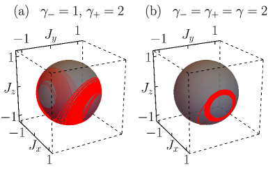
Figure 1: Evolution on the Bloch sphere of the classical open Dicke model for an initial condition near the South Pole for (a) the anisotropic and (b) the isotropic system. A chaotic attractor is seen in (a) and a limit cycle in (b). Initial condition: $(q_{0},p_{0},J_{x,y,z}^{0})=(0,0,0.001,0,-1)$. System parameters: $\omega=\omega_{0}=\kappa=1$.

Level statistics.– Just as in the case of the isolated systems, the complex eigenvalues of the Liouvillian need to be unfolded for the analysis of spectral correlations Markum et al. (1999); Akemann et al. (2019); Hamazaki et al. (2020). According to the GHS conjecture, the level spacing distribution for the unfolded spectra of dissipative systems is a 2D Poisson distribution Grobe et al. (1988); Akemann et al. (2019),

$$P_{\text{2DP}}(s)=\frac{\pi}{2}s\,e^{-\pi s^{2}/4},$$ (10)

if they show simple attractors in the classical dynamics, and it follows the Ginibre unitary ensemble (GinUE) distribution Ginibre (1965); Grobe et al. (1988); Akemann et al. (2019); Hamazaki et al. (2020)

$$P_{\text{GinUE}}(s)=\prod_{k=1}^{\infty}\frac{\Gamma(1+k,s^{2})}{k!}\sum_{k^{\prime}=1}^{\infty}\frac{2s^{2k^{\prime}+1}e^{-s^{2}}}{\Gamma(1+k^{\prime},s^{2})}$$ (11)

if the systems show chaotic attractors in the classical dynamics. In Eq. (11), $\Gamma(k,z)=\int_{z}^{\infty}dt\,t^{k-1}e^{-t}$ is the incomplete Gamma function and $\bar{s}=\int_{0}^{\infty}ds\,s\,P_{\text{GinUE}}(s)\approx 1.1429$. When comparing the distribution with numerical results, the scaling $\widetilde{P}_{\text{GinUE}}(s)=\bar{s}P_{\text{GinUE}}(\bar{s}s)$ is done to ensure that the first moment is unity, $\int_{0}^{\infty}ds\,s\,\widetilde{P}_{\text{GinUE}}(s)=1$. The degree of level repulsion is determined by the limit $s\to 0$ of the distributions above, which gives $P_{\beta}(s)\propto s^{\beta}$. Linear (cubic) level repulsion, $\beta=1$ ($\beta=3$), indicates a regular (chaotic) dissipative quantum system Haake (1991); Grobe et al. (1988); Grobe and Haake (1989).

To avoid the unfolding procedure, similarly to what is done for isolated systems Oganesyan and Huse (2007); Atas et al. (2013), the analysis of level statistics of complex eigenvalues $\lambda_{k}$ can be done with the complex spectral ratio Sá et al. (2020),

$$Z_{k}=r_{k}e^{i\theta_{k}}=\frac{\lambda_{k}^{\text{NN}}-\lambda_{k}}{\lambda_{k}^{\text{NNN}}-\lambda_{k}},$$ (12)

where NN stands for nearest neighbor and NNN for next-to-nearest neighbor. There are two limits associated with the absolute value $r_{k}=|Z_{k}|$ and the argument $\theta_{k}=\text{Arg}(Z_{k})$ of the complex ratio $Z_{k}$. For the 2D Poisson distribution, we have the average $\langle r\rangle_{\text{2DP}}=2/3$ and $-\langle\cos\theta\rangle_{\text{2DP}}=0$, while for the GinUE distribution, we have $\langle r\rangle_{\text{GinUE}}\approx 0.74$ and $-\langle\cos\theta\rangle_{\text{GinUE}}\approx 0.24$.

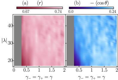
Figure 2: Analysis of the complex spectral ratio in Eq. (12) for the open isotropic Dicke model. (a) Average $\langle r\rangle$ and (b) average $-\langle\cos\theta\rangle$ as a function of the absolute values of the converged Liouvillian eigenvalues $|\lambda|$ and the coupling strength $\gamma$. The average is performed with moving windows of approximately 3000 (1000) eigenvalues for low (high) coupling strengths. Dark (light) colors indicate absence (presence) of correlated levels. The gray solid region represents the coupling values for which neither the 2DP Poisson nor the GinUE spacing distribution holds. System parameters: $\omega=\omega_{0}=\kappa=1$ and $j=2$.

The isolated classical isotropic Dicke model shows regular behavior when the excitation energies are low. Typically, for strong couplings the overall behavior is chaotic Bastarrachea-Magnani et al. (2014); Chávez-Carlos et al. (2016). The analysis of level statistics for the open version of the quantum isotropic Dicke model was done in Ref. Villaseñor and Barberis-Blostein (2024) for one value of the coupling strength $\gamma$ in the normal phase and one value in the superradiant phase. It was shown that when the isolated classical model is regular (chaotic), the complex spectrum of the Liouvillian $\hat{\mathcal{L}}_{\text{D}}$ of the open quantum model follows the 2D Poisson (GinUE) distribution.

Figure 2 extends the spectral analysis of the quantum open isotropic Dicke model for various coupling strengths $\gamma$, providing a density plot for the averages $\langle r\rangle$ [Fig. 2(a)] and $-\langle\cos\theta\rangle$ [Fig. 2(b)] as a function of $\gamma$ and the absolute values of the converged Liouvillian eigenvalues $|\lambda|$. For low coupling strengths, the low eigenvalues are mainly uncorrelated and tend to follow the 2D Poisson distribution (dark colors), while the high eigenvalues become correlated agreeing with the GinUE distribution (light colors). For large coupling strengths, the overall behavior is described by the GinUE distribution for low and high eigenvalues. In the gray region for $\gamma\to 0$, the 2D Poisson and GinUE distributions do not hold, because the system is essentially composed of two harmonic oscillators with dissipation.

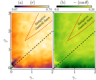
Figure 3: Analysis of the complex spectral ratio in Eq. (12) for the open anisotropic Dicke model. (a) Average $\langle r\rangle$ and (b) average $-\langle\cos\theta\rangle$ as a function of the co-rotating ($\gamma_{-}$) and counter-rotating ($\gamma_{+}$) coupling strengths. The average is performed over all converged eigenvalue absolute values $|\lambda|$ (about $10^{4}$). Dark (light) colors indicate absence (presence) of correlated levels. The red dotted lines indicate the region where chaotic attractors can be found in the classical dissipative dynamics of the anisotropic model. The diagonal black dashed line represents the isotropic Dicke model. The small gray triangle represents the coupling values for which neither the 2DP Poisson nor the GinUE spacing distribution holds. System parameters: $\omega=\omega_{0}=\kappa=1$ and $j=1$.

Breakdown of the GHS conjecture.– The fact that the open classical isotropic Dicke model only develops simple attractors [Fig. 1(b)], while its quantum counterpart can exhibit GinUE spectral correlations [Fig. 2] indicates the failure of the GHS conjecture for this experimental system. As we show next, the breakdown of the conjecture extends beyond the isotropic case.

In Fig. 3, we depict $\langle r\rangle$ and $-\langle\cos\theta\rangle$ averaged over all converged eigenvalue absolute values $|\lambda|$ as a function of the co-rotating ($\gamma_{-}$) and counter-rotating ($\gamma_{+}$) coupling strengths. Corroborating the results in Ref. Stitely et al. (2020), we mark with red dotted lines the range of values of $\gamma_{-}$ and $\gamma_{+}$ where chaotic attractors appear, which reiterates that dissipative classical chaos is only possible for this model if it is anisotropic and has large values of the coupling strengths. In contrast, the analysis of level statistics of the quantum dissipative model shows GinUE spectral correlations (light colors) for both the isotropic (black dashed line in Fig. 3) and the anisotropic case. There is a broad range of coupling strengths outside the region of dissipative classical chaos, where the eigenvalues are correlated. The appearance of chaotic attractors is not a necessary condition for the onset of level repulsion.

For completeness, we describe two special regions of system parameters in Fig. 3. The case $\gamma_{+}=0$ corresponds to the Tavis-Cummings model Tavis and Cummings (1968) with photon dissipation. The isolated classical Tavis-Cummings Hamiltonian is integrable Bastarrachea-Magnani et al. (2014), so unsurprisingly the open classical model for any value of $\gamma_{-}$ only shows simple attractors and the level statistics analysis of the quantum system indicates uncorrelated eigenvalues. The other region is the one for small values of $\gamma_{-}$, where the dominant terms of the system are counter-rotating. In this case, the degree of level repulsion increases as $\gamma_{+}$ grows, suggesting that the counter-rotating terms play an important role in the generation GinUE spectral correlations.

Discussion.– Despite the validity of the Bohigas-Giannoni-Schmit conjecture for the isolated Dicke model, we showed that the GHS conjecture fails for the open Dicke model. For a wide range of system parameters where the dissipative classical model does not exhibit chaos (absence of chaotic attractors), the dissipative quantum model can present Ginibre spectral correlations. It remains to verify whether the breakdown of the GHS conjecture is exclusive to the Dicke model or extends to other interacting spin-boson systems and even beyond. This breakdown raises two important questions: (i) If chaotic motion in a dissipative classical system is not necessarily the source of spectral correlations in the quantum domain, then what is their origin? (ii) Could there be better quantum signatures of dissipative classical chaos than level repulsion that are worth exploring, such as specific properties of dissipative out-of-time-ordered correlators García-García et al. (2024)?

Another fundamental question that emerged from our analysis concerns the classical Dicke model. It is not clear why there are regions of system parameters where the isolated model is chaotic, while the open system is not. We hope that the questions raised by our work will inspire new studies of the various aspects of quantum and classical dissipative systems.

Acknowledgments.– We acknowledge the support of the Computation Center - IIMAS, in particular to Adrián Chavesti. We also acknowledge the support of the Computation Center - ICN, in particular to Enrique Palacios, Luciano Díaz, and Eduardo Murrieta. D.V. acknowledges financial support from the postdoctoral fellowship program DGAPA-UNAM. L.F.S. is supported by the United States National Science Foundation (NSF, Grant No. DMR-1936006). P.B.-B. acknowledges support from the PAPIIT-DGAPA Grant IG101324.

References

- Bohigas et al. (1984) O. Bohigas, M. J. Giannoni, and C. Schmit, “Characterization of chaotic quantum spectra and universality of level fluctuation laws,” Phys. Rev. Lett. 52, 1–4 (1984).
- Ott (2002) Edward Ott, Chaos in Dynamical Systems (Cambridge University Press, Cambridge, UK, 2002).
- Gutzwiller (1990) M. C. Gutzwiller, Chaos in classical and quantum mechanics (Springer-Verlag, New York, 1990).
- Mehta (1991) M. L. Mehta, Random Matrices (Academic Press, Boston, MA, 1991).
- Haake (1991) Fritz Haake, Quantum Signatures of Chaos (Springer-Verlag, Berlin, 1991).
- Wimberger (2014) Sandro Wimberger, Nonlinear Dynamics and Quantum Chaos (Springer International Publishing, Switzerland, 2014).
- Guhr et al. (1998) T. Guhr, A. Müller-Groeling, and H. A. Weidenmüller, “Random matrix theories in quantum physics: Common concepts,” Phys. Rep. 299, 189 (1998).
- Berry et al. (1977) Michael Victor Berry, M. Tabor, and John Michael Ziman, “Level clustering in the regular spectrum,” Proc. Roy. Soc. London. A. Math. Phys. Sci. 356, 375–394 (1977).
- Seligman et al. (1984) T. H. Seligman, J. J. M. Verbaarschot, and M. R. Zirnbauer, “Quantum spectra and transition from regular to chaotic classical motion,” Phys. Rev. Lett. 53, 215–217 (1984).
- Seligman et al. (1985) T H Seligman, J J M Verbaarschot, and M R Zirnbauer, “Spectral fluctuation properties of Hamiltonian systems: the transition region between order and chaos,” J. Phys. A: Math. Gen. 18, 2751 (1985).
- Friedrich and Wintgen (1989) Harald Friedrich and Dieter Wintgen, “The hydrogen atom in a uniform magnetic field — an example of chaos,” Phys. Rep. 183, 37–79 (1989).
- Haake et al. (1987) F. Haake, M. Kuś, and R. Scharf, “Classical and quantum chaos for a kicked top,” Z. Phys. B Cond. Matt. 65, 381–365 (1987).
- Chaudhury et al. (2009) S. Chaudhury, A. Smith, B. E. Anderson, S. Ghose, and P. S. Jessen, “Quantum signatures of chaos in a kicked top,” Nature 461, 768–771 (2009).
- Izrailev (1990) F. M. Izrailev, “Simple models of quantum chaos: Spectrum and eigenfunctions,” Phys. Rep. 196, 299–392 (1990).
- Santhanam et al. (2022) M. S. Santhanam, Sanku Paul, and J. Bharathi Kannan, “Quantum kicked rotor and its variants: Chaos, localization and beyond,” Phys. Rep. 956, 1–87 (2022).
- Wang et al. (2022) Jiaozi Wang, Giuliano Benenti, Giulio Casati, and Wen ge Wang, “Statistical and dynamical properties of the quantum triangle map,” J. Phys. A: Math. Theor. 55, 234002 (2022).
- Hsu and Angle‘s d’Auriac (1993) Theodore C. Hsu and J. C. Angle‘s d’Auriac, “Level repulsion in integrable and almost-integrable quantum spin models,” Phys. Rev. B 47, 14291–14296 (1993).
- Santos et al. (2020) Lea F. Santos, Francisco Pérez-Bernal, and E. Jonathan Torres-Herrera, “Speck of chaos,” Phys. Rev. Res. 2, 043034 (2020).
- Benet et al. (2003) L. Benet, F. Leyvraz, and T. H. Seligman, “Wigner-dyson statistics for a class of integrable models,” Phys. Rev. E 68, 045201 (2003).
- Relaño et al. (2004) A. Relaño, J. Dukelsky, J. M. G. Gómez, and J. Retamosa, “Stringent numerical test of the poisson distribution for finite quantum integrable Hamiltonians,” Phys. Rev. E 70, 026208 (2004).
- Guckenheimer and Holmes (1983) John Guckenheimer and Philip Holmes, Nonlinear Oscillations, Dynamical Systems, and Bifurcations of Vector Fields (Springer, New York, 1983).
- Shivamoggi (2014) Bhimsen K. Shivamoggi, Nonlinear Dynamics and Chaotic Phenomena: An Introduction (Springer, Dordrecht, 2014).
- Smyrlis and Papageorgiou (1991) Y S Smyrlis and D T Papageorgiou, “Predicting chaos for infinite dimensional dynamical systems: the Kuramoto-Sivashinsky equation, a case study,” Proc. Nat. Acad. Sci. 88, 11129–11132 (1991).
- Papageorgiou and Smyrlis (1991) Demetrios T. Papageorgiou and Yiorgos S. Smyrlis, “The route to chaos for the Kuramoto-Sivashinsky equation,” Theor. Comp. Fluid Dynamics 3, 15–42 (1991).
- Grobe et al. (1988) Rainer Grobe, Fritz Haake, and Hans-Jürgen Sommers, “Quantum distinction of regular and chaotic dissipative motion,” Phys. Rev. Lett. 61, 1899–1902 (1988).
- Breuer and Petruccione (2002) H.-P. Breuer and F. Petruccione, The Theory of Open Quantum Systems (Oxford University, New York, NY, 2002).
- Carmichael (1993) Howard Carmichael, An Open Systems Approach to Quantum Optics. Lectures Presented at the Université Libre de Bruxelles, October 28 to November 4, 1991 (Springer-Verlag, Berlin, 1993).
- Carmichael (2002) H. J. Carmichael, Statistical Methods in Quantum Optics 1: Master Equations and Fokker-Planck Equations (Springer-Verlag, Berlin, 2002).
- Grobe and Haake (1989) Rainer Grobe and Fritz Haake, “Universality of cubic-level repulsion for dissipative quantum chaos,” Phys. Rev. Lett. 62, 2893–2896 (1989).
- Akemann et al. (2019) Gernot Akemann, Mario Kieburg, Adam Mielke, and Tomaž Prosen, “Universal signature from integrability to chaos in dissipative open quantum systems,” Phys. Rev. Lett. 123, 254101 (2019).
- Jaiswal et al. (2019) Ambuja Bhushan Jaiswal, Akhilesh Pandey, and Ravi Prakash, “Universality classes of quantum chaotic dissipative systems,” Europhys. Lett. 127, 30004 (2019).
- Hamazaki et al. (2019) Ryusuke Hamazaki, Kohei Kawabata, and Masahito Ueda, “Non-Hermitian many-body localization,” Phys. Rev. Lett. 123, 090603 (2019).
- Sá et al. (2020) Lucas Sá, Pedro Ribeiro, and Tomaž Prosen, “Complex spacing ratios: A signature of dissipative quantum chaos,” Phys. Rev. X 10, 021019 (2020).
- Hamazaki et al. (2020) Ryusuke Hamazaki, Kohei Kawabata, Naoto Kura, and Masahito Ueda, “Universality classes of non-Hermitian random matrices,” Phys. Rev. Res. 2, 023286 (2020).
- Rubio-García et al. (2022) Álvaro Rubio-García, Rafael A. Molina, and Jorge Dukelsky, “From integrability to chaos in quantum Liouvillians,” SciPost Phys. Core 5, 026 (2022).
- Kawabata et al. (2023) Kohei Kawabata, Anish Kulkarni, Jiachen Li, Tokiro Numasawa, and Shinsei Ryu, “Symmetry of open quantum systems: Classification of dissipative quantum chaos,” PRX Quantum 4, 030328 (2023).
- García-García et al. (2023) Antonio M. García-García, Lucas Sá, and Jacobus J. M. Verbaarschot, “Universality and its limits in non-Hermitian many-body quantum chaos using the Sachdev-Ye-Kitaev model,” Phys. Rev. D 107, 066007 (2023).
- Jaako et al. (2016) Tuomas Jaako, Ze-Liang Xiang, Juan José Garcia-Ripoll, and Peter Rabl, “Ultrastrong-coupling phenomena beyond the Dicke model,” Phys. Rev. A 94, 033850 (2016).
- Baden et al. (2014) Markus P. Baden, Kyle J. Arnold, Arne L. Grimsmo, Scott Parkins, and Murray D. Barrett, “Realization of the Dicke model using cavity-assisted Raman transitions,” Phys. Rev. Lett. 113, 020408 (2014).
- Klinder et al. (2015) Jens Klinder, Hans Keßler, Matthias Wolke, Ludwig Mathey, and Andreas Hemmerich, “Dynamical phase transition in the open Dicke model,” Proc. Nat. Ac. Sci. 112, 3290–3295 (2015).
- Zhiqiang et al. (2017) Zhang Zhiqiang, Chern Hui Lee, Ravi Kumar, K. J. Arnold, Stuart J. Masson, A. S. Parkins, and M. D. Barrett, “Nonequilibrium phase transition in a spin-1 Dicke model,” Optica 4, 424–429 (2017).
- Zhang et al. (2018) Zhiqiang Zhang, Chern Hui Lee, Ravi Kumar, K. J. Arnold, Stuart J. Masson, A. L. Grimsmo, A. S. Parkins, and M. D. Barrett, “Dicke-model simulation via cavity-assisted Raman transitions,” Phys. Rev. A 97, 043858 (2018).
- Cohn et al. (2018) J Cohn, A Safavi-Naini, R J Lewis-Swan, J G Bohnet, M Gärttner, K A Gilmore, J E Jordan, A M Rey, J J Bollinger, and J K Freericks, “Bang-bang shortcut to adiabaticity in the Dicke model as realized in a penning trap experiment,” New J. Phys. 20, 055013 (2018).
- Safavi-Naini et al. (2018) A. Safavi-Naini, R. J. Lewis-Swan, J. G. Bohnet, M. Gärttner, K. A. Gilmore, J. E. Jordan, J. Cohn, J. K. Freericks, A. M. Rey, and J. J. Bollinger, “Verification of a many-ion simulator of the Dicke model through slow quenches across a phase transition,” Phys. Rev. Lett. 121, 040503 (2018).
- Dicke (1954) R. H. Dicke, “Coherence in spontaneous radiation processes,” Phys. Rev. 93, 99 (1954).
- Garraway (2011) Barry M. Garraway, “The Dicke model in quantum optics: Dicke model revisited,” Philos. Trans. Royal Soc. A 369, 1137 (2011).
- Kirton et al. (2019) Peter Kirton, Mor M. Roses, Jonathan Keeling, and Emanuele G. Dalla Torre, “Introduction to the Dicke model: From equilibrium to nonequilibrium, and vice versa,” Adv. Quantum Techol. 2, 1800043 (2019).
- Villaseñor et al. (2024) David Villaseñor, Saúl Pilatowsky-Cameo, Jorge Chávez-Carlos, Miguel A. Bastarrachea-Magnani, Sergio Lerma-Hernández, Lea F. Santos, and Jorge G. Hirsch, “Classical and quantum properties of the spin-boson Dicke model: Chaos, localization, and scarring,” (2024), arXiv:2405.20381 [quant-ph] .
- Villaseñor and Barberis-Blostein (2024) David Villaseñor and Pablo Barberis-Blostein, “Analysis of chaos and regularity in the open Dicke model,” Phys. Rev. E 109, 014206 (2024).
- Stitely et al. (2020) Kevin C. Stitely, Andrus Giraldo, Bernd Krauskopf, and Scott Parkins, “Nonlinear semiclassical dynamics of the unbalanced, open Dicke model,” Phys. Rev. Res. 2, 033131 (2020).
- Hioe (1973) F. T. Hioe, “Phase transitions in some generalized Dicke models of superradiance,” Phys. Rev. A 8, 1440–1445 (1973).
- Hepp and Lieb (1973a) Klaus Hepp and Elliott H Lieb, “On the superradiant phase transition for molecules in a quantized radiation field: The Dicke maser model,” Ann. Phys. (N.Y.) 76, 360 – 404 (1973a).
- Hepp and Lieb (1973b) Klaus Hepp and Elliott H. Lieb, “Equilibrium statistical mechanics of matter interacting with the quantized radiation field,” Phys. Rev. A 8, 2517–2525 (1973b).
- Carmichael et al. (1973) H.J. Carmichael, C.W. Gardiner, and D.F. Walls, “Higher order corrections to the Dicke superradiant phase transition,” Phys. Lett. A 46, 47 – 48 (1973).
- Wang and Hioe (1973) Y. K. Wang and F. T. Hioe, “Phase transition in the Dicke model of superradiance,” Phys. Rev. A 7, 831–836 (1973).
- Buča and Prosen (2012) Berislav Buča and Tomaž Prosen, “A note on symmetry reductions of the Lindblad equation: transport in constrained open spin chains,” New J. Phys. 14, 073007 (2012).
- Albert and Jiang (2014) Victor V. Albert and Liang Jiang, “Symmetries and conserved quantities in Lindblad master equations,” Phys. Rev. A 89, 022118 (2014).
- Lieu et al. (2020) Simon Lieu, Ron Belyansky, Jeremy T. Young, Rex Lundgren, Victor V. Albert, and Alexey V. Gorshkov, “Symmetry breaking and error correction in open quantum systems,” Phys. Rev. Lett. 125, 240405 (2020).
- Dimer et al. (2007) F. Dimer, B. Estienne, A. S. Parkins, and H. J. Carmichael, “Proposed realization of the Dicke-model quantum phase transition in an optical cavity QED system,” Phys. Rev. A 75, 013804 (2007).
- Larson and Irish (2017) Jonas Larson and Elinor K Irish, “Some remarks on ‘superradiant’ phase transitions in light-matter systems,” J. Phys. A: Math. Theor. 50, 174002 (2017).
- Gutiérrez-Jáuregui and Carmichael (2018) R. Gutiérrez-Jáuregui and H. J. Carmichael, “Dissipative quantum phase transitions of light in a generalized Jaynes-Cummings-Rabi model,” Phys. Rev. A 98, 023804 (2018).
- Boneberg et al. (2022) Mario Boneberg, Igor Lesanovsky, and Federico Carollo, “Quantum fluctuations and correlations in open quantum Dicke models,” Phys. Rev. A 106, 012212 (2022).
- Lyu et al. (2023) Guitao Lyu, Korbinian Kottmann, Martin B. Plenio, and Myung-Joong Hwang, “Multicritical dissipative phase transitions in the anisotropic open quantum Rabi model,” (2023), arXiv:2311.11346 [quant-ph] .
- de Aguiar et al. (1992) M.A.M de Aguiar, K Furuya, C.H Lewenkopf, and M.C Nemes, “Chaos in a spin-boson system: Classical analysis,” Ann. Phys. 216, 291 – 312 (1992).
- Bastarrachea-Magnani et al. (2014) M. A. Bastarrachea-Magnani, S. Lerma-Hernández, and J. G. Hirsch, “Comparative quantum and semiclassical analysis of atom-field systems. II. Chaos and regularity,” Phys. Rev. A 89, 032102 (2014).
- Chávez-Carlos et al. (2016) J. Chávez-Carlos, M. A. Bastarrachea-Magnani, S. Lerma-Hernández, and J. G. Hirsch, “Classical chaos in atom-field systems,” Phys. Rev. E 94, 022209 (2016).
- Li et al. (2022) Jiahui Li, Rosario Fazio, and Stefano Chesi, “Nonlinear dynamics of the dissipative anisotropic two-photon Dicke model,” New J. Phys. 24, 083039 (2022).
- Li and Chesi (2024) Jiahui Li and Stefano Chesi, “Routes to chaos in the balanced two-photon Dicke model with qubit dissipation,” Phys. Rev. A 109, 053702 (2024).
- Markum et al. (1999) H. Markum, R. Pullirsch, and T. Wettig, “Non-Hermitian random matrix theory and lattice QCD with chemical potential,” Phys. Rev. Lett. 83, 484–487 (1999).
- Ginibre (1965) Jean Ginibre, “Statistical ensembles of complex, quaternion, and real matrices,” J. Math. Phys. 6, 440–449 (1965).
- Oganesyan and Huse (2007) Vadim Oganesyan and David A. Huse, “Localization of interacting fermions at high temperature,” Phys. Rev. B 75, 155111 (2007).
- Atas et al. (2013) Y. Y. Atas, E. Bogomolny, O. Giraud, and G. Roux, “Distribution of the ratio of consecutive level spacings in random matrix ensembles,” Phys. Rev. Lett. 110, 084101 (2013).
- Tavis and Cummings (1968) Michael Tavis and Frederick W. Cummings, “Exact Solution for an -Molecule—Radiation-Field Hamiltonian,” Phys. Rev. 170, 379–384 (1968).
- García-García et al. (2024) Antonio M. García-García, Jacobus J. M. Verbaarschot, and Jie ping Zheng, “The Lyapunov exponent as a signature of dissipative many-body quantum chaos,” (2024), arXiv:2403.12359 [hep-th] .