Readout Error Mitigation for Mid-Circuit Measurements and Feedforward

Abstract

Current-day quantum computing platforms are subject to readout errors, in which faulty measurement outcomes are reported by the device. On circuits with mid-circuit measurements and feedforward, readout noise can cause incorrect conditional quantum operations to be applied on a per-shot basis. Standard readout error mitigation methods for terminal measurements which act in post-processing do not suffice in this context. Here we present a general method for readout error mitigation for expectation values on circuits containing an arbitrary number of layers of mid-circuit measurements and feedforward, at zero circuit depth and two-qubit gate count cost. The protocol uses a form of gate twirling for symmetrization of the error channels and probabilistic bit-flips in feedforward data to average over an ensemble of quantum trajectories. The mitigated estimator is unbiased and has a sampling overhead of ${\sim}1/(1-2r)^{m}$ for $m$ total measurements and characteristic readout error rate $r$ per measurement. We demonstrate the effectiveness of our method, obtaining up to a ${\sim}60\%$ reduction in error on superconducting quantum processors for several examples of feedforward circuits of practical interest, including dynamic qubit resets, shallow-depth GHZ state preparation, and multi-stage quantum state teleportation.

Recent advances in quantum computing hardware have enabled the execution of mid-circuit measurements followed by subsequent quantum operations conditioned on the measurement outcomes [1, 2, 3, 4]—a capability referred to as feedforward. Quantum circuits that exploit such real-time measurement and classical logic and control capabilities have been termed dynamic circuits [5].

Dynamic capabilities are of critical importance in achieving useful quantum computation. To start, they are a prerequisite in quantum error correction [6, 7, 8, 9], which functions by way of repeated syndrome measurements and conditioned recovery operations, and thus by extension fault-tolerance. In the present noisy intermediate-scale quantum (NISQ) era, mid-circuit measurements and feedforward are also of immense utility. As they allow resetting and re-use of qubits, access to a fresh ancillary reservoir can be sustained at reduced circuit breadth and depth, hugely benefiting quantum simulation [10, 11, 12] and optimization algorithms [13]. Feedforward protocols also enable shallow-depth preparation of families of entangled quantum states, such as metrologically useful Greenberger-Horne-Zeilinger (GHZ)-like states [14, 15] and topologically ordered states [16, 17, 18, 19]. More broadly, dynamic capabilities permit performant implementations of foundational algorithmic primitives such as quantum phase estimation [5, 20], and enable classical and quantum resources to be jointly leveraged on a quantum circuit, such as in circuit knitting [21, 22], quantum state and gate teleportation [23, 24, 25], adaptive metrology [26, 27, 28], resource distillation and injection [29, 30, 31], and quantum machine learning [32] applications.

However, in practice, quantum devices exhibit readout noise [33, 34], which can lead to faulty mid-circuit measurement outcomes being reported. This, in turn, can result in incorrect quantum operations being applied during feedforward, potentially corrupting the output quantum state (Figure 1a). As these readout errors occur on a per-shot basis, and the true measurement outcomes are never known, standard readout error mitigation methods for terminal measurements [35, 36, 37], which act in post-processing and do not intervene in the execution of the quantum circuit, cannot suffice. As yet, the development of readout error mitigation techniques applicable for feedforward is an active area of research.

In this work we present probabilistic readout error mitigation (PROM), a general readout error mitigation method for quantum circuits containing mid-circuit measurements and feedforward. Our protocol leverages gate twirling for symmetrization of readout error channels and utilizes probabilistic sampling over an ensemble of minimally modified circuits to produce an unbiased estimator of arbitrary observables. The method accommodates any number of feedforward layers and incurs no circuit depth nor two-qubit gate count cost. We provide analyses on resource requirements, sensitivity, and overheads of the protocol, and experimentally demonstrate the effectiveness of the protocol on superconducting quantum processors in several settings of practical interest, namely qubit resets, shallow-depth GHZ state preparation, and multi-stage quantum state teleportation.

Our method integrates directly with probabilistic error cancellation [38, 39], which neglects readout errors, for complementary mitigation of quantum errors on dynamic circuits. More broadly any quantum error suppression or mitigation technique (e.g. Refs. [40, 41, 42, 43, 44, 45, 46, 47]) can be used in conjunction for a comprehensive targeting of hardware noise.

I Readout Errors

I.1 Basic description

Consider $m$ single-qubit computational-basis (Pauli-$Z$ basis) measurements with possible outcome bitstrings in $\mathcal{S}=\{0,1\}^{m}$. In general, readout errors affecting these $m$ measurements can be characterized by a confusion matrix $M$ [48]. Each entry $M_{ts}\in[0,1]$ records the probability that the quantum device reports measurement outcome $t\in\mathcal{S}$ when the true outcome is $s\in\mathcal{S}$. Correspondingly nonzero off-diagonal elements in $M$ indicate the presence of readout noise (see Figure 1b); in the absence of readout noise $M=\mathbb{I}$.

Suppose $\mathbf{c}$ is a vector of observed counts in an experiment, such that entry $c_{s}$ is the number of times outcome $s\in\mathcal{S}$ is observed amongst the experiment shots. Then

$$\begin{split}\mathbf{c}=M\mathbf{c}^{\prime},\end{split}$$ (1)

where $\mathbf{c}^{\prime}$ are the true counts that would hypothetically be observed without readout errors. In standard readout error mitigation (REM) methods for terminal measurements [35, 36, 37], the confusion matrix $M$ is estimated before or alongside the experiment by a calibration process. Then in post-processing, the true measurement counts $\mathbf{c}^{\prime}$ can be approximately recovered from the observed counts $\mathbf{c}$ through linear inversion, optionally with physicality constraints (see Sec. C.2 for further details).

More broadly, there exist REM techniques for terminal measurements acting in post-processing that, for example, avoids operations on $M$ by working in smaller subspaces [49] or capturing a description of readout errors based on Markov processes [50, 51]—but ultimately some form of characterization of the readout error channels is required. We thus treat the description of readout errors by $M$ as foundational.

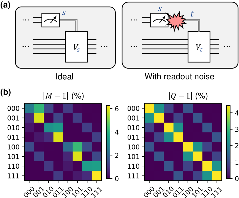
(a)

(b)

Figure 1: Readout errors. (a) In an ideal noiseless setting, a mid-circuit measurement produces an outcome $s$, which determines a subsequent quantum operation $V_{s}$ in feedforward. But in practice, readout errors can cause a measurement outcome $t$ to be reported instead, resulting in a possibly incorrect feedforward operation $V_{t}$ applied. Such errors occur on a per-shot basis and their effect cannot be corrected in post-processing. (b) Examples of the readout confusion matrix without symmetrization ($M$) and with symmetrization via bit-flip averaging ($Q$). The first column of $Q$ is the probability vector $\mathbf{q}$. The presented matrices were calibrated from superconducting quantum device ibmq_kolkata.

Layers	Assumptions	Classical Resources			Overhead $\xi^{2}$
		Init. Time	Init. Space	Sampling Time
$1$	-	$\order{m\cdot 2^{m}}$	$\order{2^{m}}$	$\order{1}$	$\norm{{\bf\it\alpha}}_{1}^{2}$
	Independent errors	$\order{m}$	$\order{m}$	$\order{m}$	$\prod_{\ell=1}^{m}(1-2r_{\ell})^{-2}$
	Uniform error	$\order{1}$	$\order{1}$	$\order{m}$	$(1-2r)^{-2m}$
$L$	-	$\order{m\cdot 2^{m}}$	$\order{2^{m}}$	$\order{1}$	$\norm{{\bf\it\alpha}}_{1}^{2}$
	Independent errors between layers	$\order{m\cdot 2^{\overline{m}}}$	$\order{L\cdot 2^{\overline{m}}}$	$\order{L}$	$\prod_{l=1}^{L}(\xi^{[l]})^{2}$
	Fully independent errors	$\order{m}$	$\order{m}$	$\order{m}$	$\prod_{\ell=1}^{m}(1-2r_{\ell})^{-2}$
	Uniform error	$\order{1}$	$\order{1}$	$\order{m}$	$(1-2r)^{-2m}$

Table 1: Summary of characteristics of the probabilistic readout error mitigation protocol (PROM) studied in this paper. Above $m$ is the total number of mid-circuit measurements and $\overline{m}$ is the maximum number of measurements in a feedforward layer. Under independence assumptions, $r_{\ell}\in[0,1/2)$ are characteristic readout error probabilities for measurement $\ell\in[m]$, and under uniformity assumptions $r_{\ell}=r$ identically. The ‘Init. Time’ and ‘Init. Space’ columns refer to initial classical time and memory costs of computing coefficients for the mitigated estimator, ‘Sampling Time’ refers to the classical sampling time to generate a bitmask per experiment shot (see Sec. II.1), and ‘Overhead’ refers to a multiplicative factor in the number of experiment shots required for the mitigated estimator to converge to the same precision at the same confidence as hypothetical noiseless circuit execution. The single-layer variants are special cases of the multi-layer variants.

I.2 Symmetrization of readout errors

Generically $M$ is stochastic but not symmetric ($M\neq M^{\mathsf{T}}$) and is characterized by $\absolutevalue{\mathcal{S}}(\absolutevalue{\mathcal{S}}-1)=2^{m}(2^{m}-1)$ independent parameters. However, a twirling technique, named bit-flip averaging (BFA), can be used to symmetrize the readout error channels [52, 53], thus simplifying their description. In the BFA scheme, for every shot of the circuit, each measurement is randomly sandwiched between a pair of inserted $X$ gates and a corresponding classical bit-flip is applied to the outcome of the measurement. The first $X$ coherently flips the state of the qubit ($\ket{0}\leftrightarrow\ket{1}$), which is measured and the classical bit-flip restores the measurement outcome; the second $X$ restores the post-measurement quantum state in case further quantum operations occur on the qubit, and can be excluded for terminal measurements.

With BFA applied, the symmetrized effective readout error channels are characterized by a probability distribution $\mathbf{q}$. Each entry $q_{s}\in[0,1]$ records the probability of the error syndrome $s\in\mathcal{S}$ occurring, that is, the probability of reporting outcome $(a\oplus s)\in\mathcal{S}$ when the true outcome is $a\in\mathcal{S}$, where $\oplus$ denotes the binary sum or XOR of two bitstrings. Nonzero $q_{s}$ for $s\neq\mathbf{0}$ indicate the presence of readout noise; in the absence of readout noise $q_{s}=\delta_{s\mathbf{0}}$.

Compared to $M$ without symmetrization, $\mathbf{q}$ contains $\absolutevalue{\mathcal{S}}-1=2^{m}-1$ independent parameters. This reduced description is without loss of generality—$\mathbf{q}$ still accommodates arbitrary correlations in readout errors. Conceptually, this symmetrization of readout errors is similar to that of quantum processes by gate twirling [54], for example, the diagonalization of arbitrary quantum channels into incoherent Pauli channels [55, 56, 57, 58, 59], which is exploited in probabilistic error cancellation [38, 39] and randomized compilation of quantum circuits [45, 46]. In our present work, we assume that BFA is always applied.

Lastly, we consider also the associated symmetrized confusion matrix $Q$ with entries $Q_{sf}=q_{s\oplus f}$ for $s,f\in\mathcal{S}$ (see Figure 1b). The first column of $Q$ is $\mathbf{q}$, which completely specifies $Q$. To lay a concrete intuition, with these definitions, the relation between observed $\mathbf{c}$ and true counts $\mathbf{c}^{\prime}$ in Eq. 1 becomes

$$\begin{split}\mathbf{c}=\mathbf{c}^{\prime}\ast\mathbf{q}\Longleftrightarrow\mathbf{c}=Q\mathbf{c}^{\prime},\end{split}$$ (2)

where $\ast$ denotes convolution. In general, the readout error probabilities $\mathbf{q}$, and hence $Q$, are straightforward to characterize in experiments (see Sec. C.2).

By construction $Q$ is hugely symmetric—in particular, $Q$ is symmetric about both its diagonal and anti-diagonal, and so is every of its recursively halved quadrants. Thus $Q\in\mathrm{span}(\{\mathbb{I},X\}^{\otimes m})$ and has closed-form eigenvalues

$$\begin{split}\lambda_{k}=\sum_{s\in\mathcal{S}}(-1)^{k\cdot s}q_{s}=1-2\sum_{\begin{subarray}{c}s\in\mathcal{S}\\ k\cdot s\neq 0\end{subarray}}q_{s},\end{split}$$ (3)

for each $k\in\mathcal{S}$, or equivalently ${\bf\it\lambda}=\mathcal{W}(\mathbf{q})$ where $\mathcal{W}$ is the unnormalized Walsh-Hadamard transform [60, 61], which can be regarded as a generalized Fourier transform. A derivation of this result and technical details are included in Sec. A.3. We note $\lambda_{\mathbf{0}}=1$ and $\lambda_{k}\leq 1$ generically for $k\neq\mathbf{0}$; in the noiseless limit $\lambda_{k}=1$ uniformly.

II Protocol for Single Feedforward Layer

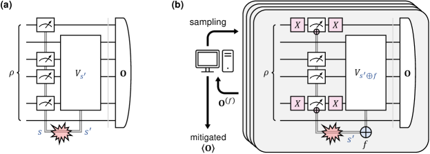
(a)

(b)

Figure 2: Probabilistic readout error mitigation for a single feedforward layer. (a) Structure of the quantum circuit considered, comprising state preparation, a layer of mid-circuit measurements and feedforward, and terminal measurements of observables $\mathbf{O}$. From shot to shot, the correct measurement outcome (bitstring) $s$ is corrupted into $s^{\prime}$ by readout errors, and the reported outcome $s^{\prime}$ conditions the feedforward unitary $V_{s^{\prime}}$ that is applied. (b) Schematic of our readout error mitigation protocol. Bit-flip averaging is applied by randomly twirling measurements with quantum and classical $X$ gates (shaded pink), and the XOR between the reported measurement outcome and a bitmask $f$ is used for feedforward. By sampling $f$ over a suitable probability distribution and with some classical post-processing, mitigated expectation values of $\mathbf{O}$ are produced.

To start, we consider REM applicable to circuits with a single mid-circuit measurement and feedforward layer. The setup considered here is (see Figure 2a):

1. A quantum state $\rho$ is prepared.

2. Mid-circuit measurements are performed in the computational basis on some subset of $m$ qubits. The correct measurement outcome is $s\in\mathcal{S}=\{0,1\}^{m}$, but readout errors cause $s^{\prime}\in\mathcal{S}$ to be reported.

3. The reported measurement outcome $s^{\prime}$ feedforwards into a unitary $V_{s^{\prime}}$. In the quantum circuit specification a complete set of feedforward unitaries $\{V_{s}\}_{s\in\mathcal{S}}$ is accordingly assumed to be specified.

4. Observables $\mathbf{O}=\matrixquantity[O_{1}&O_{2}&\ldots&O_{B}]$ are measured. We assume $\smash{\norm*{O_{b}}_{2}\leq 1\,\forall\,b\in[B]}$.

We remark that this setup makes minimal assumptions. Over a number of circuit execution shots, statistics on the outcomes of the $\mathbf{O}$ measurements are collected and the expectation values $\expectationvalue{\mathbf{O}}$ calculated. We denote the ideal noiseless (wherein $s=s^{\prime}$ for all shots) expectation values as $\smash{\expectationvalue{\overline{\mathbf{O}}}}$.

Readout errors on the mid-circuit measurements can cause incorrect feedforward unitaries (where $s\neq s^{\prime}$) to be applied in each shot, thus corrupting the quantum state and producing $\expectationvalue{\mathbf{O}}\neq\smash{\expectationvalue{\overline{\mathbf{O}}}}$. Standard REM methods for terminal measurements [35, 36, 37] that act in post-processing cannot mitigate these errors, as they do not restore the broken correlations between the mid-circuit measurement outcomes and feedforward operations. We present a REM protocol that addresses this issue.

In our prescription, while the mid-circuit measurements are subject to readout errors, we neglect readout noise on the $\mathbf{O}$ measurements themselves, for standard REM methods for terminal measurements can be readily applied.

II.1 Readout error mitigation protocol

Consider that on reported mid-circuit measurement outcome $s^{\prime}\in\mathcal{S}$, the feedforward unitary $V_{s^{\prime}\oplus f}$ for a bitmask $f\in\mathcal{S}$ is applied instead of $V_{s^{\prime}}$. We denote the $\mathbf{O}$ observables measured in this setting as $\smash{\mathbf{O}^{(f)}}$. We define the estimator

$$\begin{split}\widehat{\mathbf{O}}\coloneqq\sum_{f\in\mathcal{S}}\alpha_{f}\mathbf{O}^{(f)}=\xi\sum_{f\in\mathcal{S}}\frac{\absolutevalue{\alpha_{f}}}{\xi}\operatorname*{sgn}(\alpha_{f})\mathbf{O}^{(f)},\end{split}$$ (4)

where coefficients $\alpha_{f}\in\mathbb{R}$ are to be found such that $\smash{\widehat{\mathbf{O}}}$ is an unbiased estimator of $\smash{\overline{\mathbf{O}}}$, that is, $\smash{\expectationvalue*{\widehat{\mathbf{O}}}=\expectationvalue*{\overline{\mathbf{O}}}}$. As shorthand we write $\smash{{\bf\it\alpha}=\smash{\matrixquantity[\alpha_{\mathbf{0}}&\ldots&\alpha_{\mathbf{1}}]}^{\mathsf{T}}}$, and $\xi=\smash{\norm*{{\bf\it\alpha}}_{1}}=\smash{\sum_{f\in\mathcal{S}}\absolutevalue{\alpha_{f}}}$. Note that the entries of ${\bf\it\alpha}$ need not be positive. Supposing that a solution for ${\bf\it\alpha}$ is available, $\smash{\expectationvalue*{\widehat{\mathbf{O}}}}$ can be measured through a sampling procedure (see Figure 2b):

1. For each experiment shot, randomly sample a bitmask $f\in\mathcal{S}$ with probability $\absolutevalue*{\alpha_{f}}/\xi$, and execute the circuit with $f$ applied in the feedforward. At the end of the shot, multiply the $\mathbf{O}$ results by $\operatorname*{sgn}(\alpha_{f})$.

2. Take the average of the $\mathbf{O}$ results from all shots and multiply by $\xi$.

Standard statistical analysis indicates that this mitigated protocol for measuring $\mathbf{O}$ carries a sampling overhead of $\xi^{2}$ compared to a hypothetical noiseless experiment. That is, to obtain the same precision of measured $\expectationvalue{\mathbf{O}}$ at the same confidence as $N$ hypothetical noiseless shots, a number of noisy shots scaling as $\xi^{2}N$ is sufficient. Moreover, under general conditions, for a total readout error probability $\eta=1-q_{\mathbf{0}}<1/2$, the overhead factor can be shown to satisfy $\xi<1/(1-2\eta)$. We refer readers to Secs. B.3 and B.4 for the derivation of these results.

II.2 General solution

We now outline the main ideas leading to a solution for the sampling coefficients ${\bf\it\alpha}$ in the protocol. To start, in a picture of quantum trajectories, the quantum state after the mid-circuit measurements and feedforward in the absence of readout errors can be written as

$$\begin{split}\overline{\sigma}=\sum_{s\in\mathcal{S}}p_{s}V_{s}\rho_{s}V_{s}^{\dagger},\end{split}$$ (5)

where each trajectory is defined by the measurement outcome $s$ and results in a normalized quantum state $\smash{\rho_{s}=(\Pi_{s}\rho\Pi_{s})/p_{s}}$ when $p_{s}\neq 0$. Here $\Pi_{s}$ is the measurement projector associated with the outcome $s$, and the probability of that trajectory occurring is $\smash{p_{s}=\tr(\Pi_{s}\rho)}$. It is useful to define the tensor

$$\begin{split}T_{bss^{\prime}}=p_{s}\tr\left(O_{b}V_{s^{\prime}}\rho_{s}V_{s^{\prime}}^{\dagger}\right),\end{split}$$ (6)

such that the entry $T_{bss^{\prime}}$ is the expectation value of $O_{b}$ measured on quantum trajectories that had measurement outcome $s$ but feedforward unitary $\smash{V_{s^{\prime}}}$ applied, weighted by the probability $p_{s}$ of those trajectories occurring. Thus, the diagonal and off-diagonal entries of the matrix $T_{b}$ describe trajectories in which feedforward is correctly and incorrectly performed, respectively. Then

$$\begin{split}\expectationvalue{\overline{O}_{b}}=\tr\left(O_{b}\overline{\sigma}\right)=\tr T_{b}.\end{split}$$ (7)

Now we consider the presence of readout errors. On a per-shot basis, a true mid-circuit measurement outcome $s$ is corrupted into $s^{\prime}$, and in addition we impose a bitmask $f\in\mathcal{S}$ such that feedforward unitary $V_{s^{\prime}\oplus f}$ is applied. The quantum state after the mid-circuit measurements and feedforward is

$$\begin{split}\sigma^{(f)}=\sum_{s\in\mathcal{S}}\sum_{s^{\prime}\in\mathcal{S}}q_{s\oplus s^{\prime}}p_{s}V_{s^{\prime}\oplus f}\rho_{s}V_{s^{\prime}\oplus f}^{\dagger},\end{split}$$ (8)

where $q_{s\oplus s^{\prime}}$ is the probability of the readout error occurring (as described in Sec. I.2). Accordingly

$$\begin{split}\expectationvalue{O_{b}^{(f)}}=\tr\left(O_{b}\sigma^{(f)}\right)&=\sum_{s\in\mathcal{S}}\sum_{s^{\prime}\in\mathcal{S}}q_{s\oplus s^{\prime}}T_{bs(s^{\prime}\oplus f)}.\end{split}$$ (9)

Desiring an unbiased estimator $\smash{\expectationvalue*{\widehat{\mathbf{O}}}=\expectationvalue*{\overline{\mathbf{O}}}}$, we substitute Eq. 7 and Eq. 9 into Eq. 4. This results in an equality that is enforced for every $b\in[B]$. We do not assume further knowledge of the problem at hand; thus, the tensor $T$ is unknown and the mitigation protocol must work for arbitrary $T$. Then the equality necessitates that the coefficients of every $T_{bss^{\prime}}$ match on both sides. This yields a linear system encoding a unique ${\bf\it\alpha}$, with closed-form solution

$$\begin{split}\alpha_{f}=\frac{1}{2^{m}}\sum_{k\in\mathcal{S}}(-1)^{f\cdot k}\left(\frac{1}{\lambda_{k}}\right),\end{split}$$ (10)

where ${\bf\it\lambda}$ are eigenvalues of $Q$ as obtained in Eq. 3. Equivalently, ${\bf\it\alpha}=\mathcal{W}(\mathbf{1}/{\bf\it\lambda})/2^{m}$ for $\mathcal{W}$ the unnormalized Walsh-Hadamard transform. A full derivation of this result, and alternate forms for ${\bf\it\alpha}$, are given in Sec. B.1.1. In the noiseless limit $\alpha_{\mathbf{0}}=\delta_{f\mathbf{0}}$ and $\xi=1$.

In this general setting there are ${\sim}2^{m}$ independent entries of ${\bf\it\alpha}$ to be computed, which demand classical resources scaling exponentially in $m$. But, thereafter, using standard algorithms [62, 63, 64] to sample from the computed probability distribution, the drawing of bitmasks $f\in\mathcal{S}$ can be performed in constant time per shot. These complexities are summarized in Table 1, with further details elaborated in Sec. B.1.1.

A pertinent further question concerns the sensitivity or well-conditionedness of the mitigation protocol. That is, given differing $\mathbf{q}$ and $\mathbf{q}^{\prime}$ inputs characterizing the readout errors present, how large are the differences in the mitigated expectation values $\smash{\expectationvalue*{\widehat{\mathbf{O}}^{\prime}}}$ and $\smash{\expectationvalue*{\widehat{\mathbf{O}}}}$, and secondarily the overhead factors $\xi$ and $\xi^{\prime}$? This question is relevant as in reality, calibration of $\mathbf{q}$ on a quantum device inevitably carries small errors up to a finite experimental precision; moreover, it may be desirable to employ approximations on $\mathbf{q}$, for example as described next in Sec. II.3. We show that small errors in inputs propagate mildly through the protocol. Specifically,

$$\absolutevalue{\expectationvalue{\widehat{O}^{\prime}_{b}}-\expectationvalue{\widehat{O}_{b}}} \leq\frac{2\xi^{2}d}{1-2\xi d},$$ (11a)

$$\absolutevalue{\xi^{\prime}-\xi} \leq\frac{2\xi^{2}d}{1-2\xi d},$$ (11b)

where $d$ is the total variation distance between $\mathbf{q}$ and $\mathbf{q}^{\prime}$, for $2\xi d<1$. In particular, taking $\mathbf{q}^{\prime}$ as the (unknown) exact characterization and $\mathbf{q}$ the characterization used in the mitigation protocol, the error in mitigated observables scale linearly as ${\sim}2\xi^{2}d$ to leading order, where $d$ is small given sufficiently good calibration of readout error probabilities on the device.

Secondarily, suppose that the characterized readout errors $\mathbf{q}$ on the quantum device contain small correlations, but the errors are otherwise close to being independent. Then Eq. 11b implies that the overhead factor of the mitigation protocol is close to that assuming independent errors, which is easy to evaluate, as analyzed next in Sec. II.3. We refer readers to Sec. B.4 for derivations of the sensitivity bounds above.

II.3 Simplified solutions

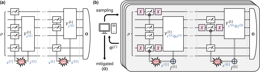
(a)

(b)

Figure 3: Probabilistic readout error mitigation for multiple feedforward layers. (a) Structure of the quantum circuit considered, comprising state preparation, $L$ layers of mid-circuit measurements and feedforward, and terminal measurements of observables $\mathbf{O}$. From shot to shot, in layer $l$, the correct measurement outcome (bitstring) $\smash{s^{[l]}}$ is corrupted into $\smash{s^{\prime[l]}}$ by readout errors, and the reported outcome $\smash{s^{\prime[l]}}$ determines a feedforward unitary $\smash{V^{[l]}_{s^{\prime[l]}}}$ that is applied. (b) Schematic of our readout error mitigation protocol. Bit-flip averaging is applied by randomly twirling measurements with quantum and classical $X$ gates (shaded pink), and in layer $l$ the XOR between the reported measurement outcome and a bitmask $\smash{f^{[l]}}$ is used for feedforward. By sampling $\smash{f=f^{[1]}f^{[2]}\ldots f^{[L]}}$ over a suitable probability distribution and with some classical post-processing, mitigated expectation values of $\mathbf{O}$ are produced.

In a setting where readout errors affecting the $m$ mid-circuit measurements are assumed to be independent, the solution for ${\bf\it\alpha}$ factorizes,

$$\begin{split}{\bf\it\alpha}=\bigotimes_{\ell=1}^{m}{\bf\it\alpha}^{(\ell)},\qquad{\bf\it\alpha}^{(\ell)}=\frac{1}{1-2r_{\ell}}\matrixquantity[1-r_{\ell}\\ -r_{\ell}],\end{split}$$ (12)

where $r_{\ell}\in[0,1/2)$ is the readout error probability for the $\ell^{\text{th}}$ measurement. Writing $\smash{\xi^{(\ell)}=\norm*{{\bf\it\alpha}^{(\ell)}}_{1}}$, the overhead factor may be expressed as:

$$\begin{split}\xi=\prod_{\ell=1}^{m}\xi^{(\ell)}=\prod_{\ell=1}^{m}\frac{1}{1-2r_{\ell}}.\end{split}$$ (13)

The factorized structure of ${\bf\it\alpha}$ implies that $\absolutevalue*{{\bf\it\alpha}}/\xi$ is a product over individual $\absolutevalue*{{\bf\it\alpha}^{(\ell)}}/\xi^{(\ell)}$ probability distributions. This enables a reduction of classical resources required to initialize the mitigation protocol to $\order{m}$ time and space, with $\order{m}$ sampling time for each shot. In an even simpler setting of uniform readout channels ($r_{\ell}=r$), all $\smash{{\bf\it\alpha}^{(\ell)}}$ are identical and classical initialization costs are trivially reduced to $\order{1}$ time and space. These complexities are reflected in Table 1, and further technical details are provided in Sec. B.1.2.

In practice, readout errors on a quantum device expectedly exhibit at least a small amount of correlations or non-uniformity. How large would the consequences of assuming independence or uniformity be? Our prior discussion surrounding Eq. 11a has established a mild scaling of errors in the mitigated observables versus ideal values, with respect to the (small) total variation distance between the true $\mathbf{q}$ and that used in the protocol. For small distances, errors made by an approximate mitigation assuming independence or uniformity remain small—and importantly, the approximation enables significant resource complexity savings against the general setting. The utility of such simplifications thus depends on the quantum device and the scale of the problem at hand. We discuss this further in our experimental study in Sec. IV.

III Protocol for Multiple Feedforward Layers

We now consider the more general scenario of having $L$ feedforward layers. The single-layer context discussed in Sec. II is subsumed as a special case with $L=1$. The setup considered is (see Figure 3a):

1. A quantum state $\rho$ is prepared.

2. For layer $l\in[L]$:

   1. Mid-circuit measurements are performed in the computational basis on some subset of $\smash{m^{[l]}}$ qubits. The correct measurement outcome is $\smash{s^{[l]}\in\mathcal{S}^{[l]}}=\smash{\{0,1\}^{m^{[l]}}}$, but readout errors cause $\smash{s^{\prime[l]}\in\mathcal{S}^{[l]}}$ to be reported.

   2. The reported measurement outcome $\smash{s^{\prime[l]}}$ feedforwards into a unitary $\smash{V^{[l]}_{s^{\prime[l]}}}$. In the quantum circuit specification a complete set of feedforward unitaries $\smash{\{V^{[l]}_{s}\}_{s\in\mathcal{S}^{[l]}}}$ is accordingly assumed to be specified.

3. Observables $\mathbf{O}=\matrixquantity[O_{1}&O_{2}&\ldots&O_{B}]$ are measured. We assume $\smash{\norm*{O_{b}}_{2}\leq 1\,\forall\,b\in[B]}$.

As before, we remark that this setup makes minimal assumptions. For consistency with our prior notation, we denote the total number of mid-circuit measurements $\smash{m=\sum_{l=1}^{L}m^{[l]}}$, and the set of outcomes over all measurements $\smash{\mathcal{S}=\mathcal{S}^{[1]}\times\mathcal{S}^{[2]}\times\ldots\times\mathcal{S}^{[L]}=\{0,1\}^{m}}$.

On the quantum device, readout errors on the mid-circuit measurements in each layer can cause incorrect feedforward unitaries to be applied, thus producing a measured $\expectationvalue{\mathbf{O}}$ that differs from the ideal noiseless $\expectationvalue{\overline{\mathbf{O}}}$. We seek a protocol that reduces this deviation. As before, we neglect readout noise on the $\mathbf{O}$ measurements themselves, for standard REM methods for terminal measurements can be readily applied [35, 36, 37].

III.1 Readout error mitigation protocol

We define the mitigated estimator $\widehat{\mathbf{O}}$ and invoke a protocol exactly identical to Sec. II.1. Operationally, in each experiment shot, we partition the sampled bitmask $\smash{f=f^{[1]}f^{[2]}\ldots f^{[L]}}\in\mathcal{S}$ into layer-wise bitmasks $\smash{f^{[l]}\in\mathcal{S}^{[l]}}$, and we apply $f^{[l]}$ to the feedforward in layer $l$. It follows that the sampling overhead is identical at $\xi^{2}=\norm*{{\bf\it\alpha}}_{1}^{2}$, as analyzed in Sec. B.3. When the total readout error probability $\eta<1/2$, the general bound that $\xi<1/(1-2\eta)$ likewise applies.

III.2 General solution

In a similar fashion to the single-layer context in Sec. II.2, we outline a general solution for ${\bf\it\alpha}$. With $\smash{s=s^{[1]}s^{[2]}\ldots s^{[L]}\in\mathcal{S}}$ the concatenation of measurement outcomes across all layers and $\smash{\Pi^{[l]}_{s^{[l]}}}$ the measurement projector in layer $l$ associated with the outcome $\smash{s^{[l]}}$, we write the sequence $W$ of mid-circuit measurements and feedforward unitaries, and likewise define the tensor $T$,

$$\begin{split}W_{ss^{\prime}}=\prod_{l=L}^{1}V^{[l]}_{s^{\prime[l]}}\Pi^{[l]}_{s^{[l]}},\quad T_{bss^{\prime}}=\tr\left[O_{b}W_{ss^{\prime}}\rho W_{ss^{\prime}}^{\dagger}\right].\end{split}$$ (14)

Directly analogous to Eq. 6, the entry $T_{bss^{\prime}}$ is the expectation value of $O_{b}$ measured on quantum trajectories that had true measurement outcomes $s$ but feedforward unitaries applied according to $s^{\prime}$, weighted by the probability of those trajectories occurring.

Then the ideal expectation value of $O_{b}$ in a hypothetical noiseless setting, $\smash{\expectationvalue*{\overline{O}_{b}}}$, has exactly the same form as in Eq. 7 but with $T$ defined above. Moreover, the expectation value of $O_{b}$ with readout errors and with bitmask $f\in\mathcal{S}$ applied in the feedforward, $\smash{\expectationvalue*{O_{b}^{(f)}}}$, has the same form as in Eq. 9. Just as in Sec. II.2, we demand $\smash{\expectationvalue*{\widehat{\mathbf{O}}}=\expectationvalue*{\overline{\mathbf{O}}}}$ and thus equate $\smash{\expectationvalue*{\overline{O}_{b}}}$ and $\smash{\expectationvalue*{O_{b}^{(f)}}}$ through the definition of $\smash{\widehat{\mathbf{O}}}$, leading to a requirement that the coefficient of every $T_{bss^{\prime}}$ match on both sides.

As $\smash{\expectationvalue*{\overline{O}_{b}}}$ and $\smash{\expectationvalue*{O_{b}^{(f)}}}$ have remained identical in form, we have the same solution for ${\bf\it\alpha}$—namely, that given in Eq. 10. We provide an explicit derivation and further technical details in Sec. B.2.1. The classical resource costs are likewise unchanged and are listed in Table 1, and the protocol sensitivity results in Eqs. 11a and 11b identically apply.

III.3 Simplified solutions

As the measurements in different layers of the circuit are separated in time, a plausible assumption is that readout errors affecting them are independent, consistent with standard Markovian assumptions on noise channels [65, 66]. Measurements within the same layer, which may occur simultaneously or in overlapping time intervals, may still exhibit correlations in errors. In such a setting, the confusion vector $\mathbf{q}$ factorizes and so do the solutions for ${\bf\it\lambda}$ and ${\bf\it\alpha}$,

$$\begin{split}\mathbf{q}=\bigotimes_{l=1}^{L}\mathbf{q}^{[l]},\qquad{\bf\it\lambda}=\bigotimes_{l=1}^{L}{\bf\it\lambda}^{[l]},\qquad{\bf\it\alpha}=\bigotimes_{l=1}^{L}{\bf\it\alpha}^{[l]},\end{split}$$ (15)

where $\smash{k=k^{[1]}k^{[2]}\ldots k^{[L]}}\in\mathcal{S}$ and $\smash{f=f^{[1]}f^{[2]}\ldots f^{[L]}}\in\mathcal{S}$ partition the bitstrings over the layers, and $\smash{\mathbf{q}^{[l]}}$, $\smash{{\bf\it\lambda}^{[l]}}$ and $\smash{{\bf\it\alpha}^{[l]}}$ are the confusion vector, eigenvalues and mitigator coefficients for layer $l$ respectively. Explicitly, the latter two are given by Eqs. 3 and 10 but with $(\mathcal{S},m,\mathbf{q},k,f)$ replaced by their layer counterparts $\smash{(\mathcal{S}^{[l]},m^{[l]},\mathbf{q}^{[l]},k^{[l]},f^{[l]})}$. Writing layer-wise overheads $\smash{\xi^{[l]}=\norm*{{\bf\it\alpha}^{[l]}}_{1}}$, the overhead factor likewise factorizes,

$$\begin{split}\xi=\prod_{l=1}^{m}\xi^{[l]}.\end{split}$$ (16)

Then $\absolutevalue{{\bf\it\alpha}}/\xi$ is a product over the layer-wise $\smash{\absolutevalue*{{\bf\it\alpha}^{[l]}}/\xi^{[l]}}$ probability distributions. This allows a reduction of the classical resources required to $\smash{\order*{m\cdot 2^{\overline{m}}}}$ time and $\smash{\order*{L\cdot 2^{\overline{m}}}}$ space for solution computation, where $\smash{\overline{m}=\max_{l\in[L]}m^{[l]}}$ is the maximum number of measurements in a layer, and $\order{L}$ classical sampling time per shot, as summarized in Table 1. Further analysis details are provided in Sec. B.2.2.

For yet further simplification, a stronger assumption is to impose independence on readout errors across all measurements regardless of their location in layers, and even stronger still, to assume that all readout error channels are uniform. These settings enforce additional structure in the solutions and land us in the context of Sec. II.3. The results for ${\bf\it\alpha}$ and classical resource costs there directly apply.

IV Hardware Experiments

To demonstrate the effectiveness of our probabilistic readout error mitigation (PROM) strategy, we executed a series of experiments on $27$- and $127$-qubit IBM transmon-based superconducting quantum processors. These devices support mid-circuit measurements and feedforward, and have characteristic readout error rates of $0.5$–$3\%$ per measurement. As there is clear non-uniformity in readout error rates between qubits, we examine both general PROM and PROM assuming independent readout errors, but we omit further uniformity assumptions. We provide more details on the quantum hardware used in Sec. C.1, with device specifications listed in Table S2. Our experiments span dynamic qubit reset, shallow-depth GHZ state preparation, and repeated quantum state teleportation (Secs. IV.1, IV.2 and IV.3), thus covering a variety of use-cases of practical interest.

Our experiments employ PROM for mid-circuit measurements and feedforward, in conjunction with standard REM for terminal measurements (see Sec. C.2). We clearly distinguish results with terminal REM only, and with both PROM and terminal REM. We implement dynamical decoupling on all circuits to suppress decoherence on idle qubits (see Sec. C.3).

For comparison, we examine also a repetition-based REM strategy for feedforward. The strategy works by performing each mid-circuit measurement $r>1$ times consecutively and taking a consensus outcome for feedforward, such that the readout error rate perceived by the feedforward is suppressed. This general approach is commonly invoked in quantum error correction and fault-tolerant quantum computation [67, 6]. For our purposes, we consider two variants—Rep-MAJ, which takes the majority outcome for odd $r$, and Rep-ALL, which requires agreement between all measurement outcomes for feedforward to go through and discards the experiment shot otherwise (i.e. post-selection).

Notably, PROM differs from these repetition-based methods in that PROM does not modify the quantum circuit to be executed. The repetition-based methods, on the other hand, increase the number of measurements and depth of the circuit. This difference has non-trivial implications in practice, as we shall observe.

To start, we demonstrate PROM in the context of dynamic qubit resets. A reset is a (non-unitary) operation that re-initializes a qubit to $\ket{0}$ regardless of the input state [68, 69]; on digital quantum processors, it can be implemented as a mid-circuit measurement followed by an $X$ gate conditioned on a $1$ outcome. As they enable arbitrary re-use of qubits, resets are of pivotal utility across quantum algorithms, simulation, optimization and metrology domains [12, 70, 71]. Concretely, qubit resets have enabled long-time simulations of open quantum systems [10, 11], execution of wide quantum approximate optimization algorithm (QAOA) circuits on present hardware [13], and have been leveraged in phase estimation [5] and spectroscopy techniques [72]. More broadly, resets serve as an entropy sink in measurement-free quantum error correction protocols [73, 74], and are generally useful in quantum algorithms that repeatedly access (and discard into) an ancillary reservoir [75, 76, 77, 78].

IV.1 Mid-circuit dynamic qubit reset

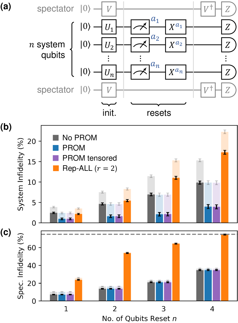
(a)

(b)

(c)

Figure 4: Dynamic qubit resets. (a) Circuit structure to probe fidelity of qubit reset operations. A register of $n$ system qubits (black) undergo evolution by $U_{1}\otimes\cdots\otimes U_{n}$ and are then reset into the $\smash{\ket{0}^{\otimes n}}$ state. A pair of adjacent spectator qubits (gray) sandwiching the system register witness the reset events. Dynamic resets are implemented as mid-circuit measurements followed by $X$ gates conditioned on outcomes (blue labels). (b) Infidelities of system qubits after dynamic resets against $\smash{\ket{0}^{\otimes n}}$, comparing PROM, PROM assuming tensored readout error channels, Rep-ALL at $r=2$, and without readout error mitigation for mid-circuit measurements and feedforward. (c) Infidelities of spectator qubits against $\smash{\ket{0}^{\otimes 2}}$ after witnessing reset events, conditioned on the system qubits being reset correctly. Dashed line demarcates $75\%$ infidelity expected for a maximally mixed spectator state. In all plots, solid bars are with terminal readout error mitigation; translucent bars without. Experiments performed on superconducting quantum device ibmq_kolkata. Error bars are standard deviations across $1000$ trials per qubit chain, each with $10000$ shots; data averaged over ${\sim}8$ randomly chosen qubit chains.

The circuit structure we examine comprises $n$ system qubits that are prepared in $(U_{1}\otimes U_{2}\otimes\cdots\otimes U_{n})\ket{0}^{\otimes n}$, dynamically reset, and then terminally measured to verify their post-reset state (see Figure 4a). A pair of spectator qubits sandwiches the system register and are each prepared in $V\ket{0}$. After witnessing the resets on the system qubits, they are back-rotated by $V^{\dagger}$ and measured. In an ideal noiseless setting, the terminal states of the system and spectator qubits should all be $\ket{0}$. To probe the fidelity of the reset operations, our observables $\mathbf{O}$ thus constitute $\smash{\ket{0}^{\otimes n}\bra{0}^{\otimes n}}$ on the system qubits and $\smash{\ket{0}^{\otimes 2}\bra{0}^{\otimes 2}}$ on the spectator qubits. In our experiments, we place all qubits on a contiguous chain on the quantum processor, and we take $U_{1}=\cdots=U_{n}=V=H$.

We present in Figure 4b system infidelities against the ideal $\ket{0}^{\otimes n}$ post-reset state, for $n\in\{1,2,3,4\}$ qubits. We compare data without PROM, with general PROM and PROM under an assumption of tensored readout error channels, and with Rep-ALL at $r=2$. The drastic effect of PROM is evident—our protocol reduces system infidelities to ${\sim}30$–$40\%$ of their unmitigated values. In contrast to PROM, the repetition-based Rep-ALL scheme does not appreciably improve, and in fact worsens for $n>1$, system fidelities across the board.

While PROM addresses readout errors affecting feedforward, on hardware a variety of other noise sources are present (e.g. gate errors and decoherence), which account for the observed residual infidelities. As discussed, in sensitive applications, PROM can be used in conjunction with other error mitigation techniques that complementarily address these other noise sources. In Figure 4b we have also reported data without terminal REM, drawn as translucent bars. The observed fidelity improvements provided by terminal REM alone (without PROM) and by the addition of PROM are comparable, indeed expected as there are equal numbers of mid-circuit and terminal measurements on the system qubits ($n$ each).

An additional layer of contrast is unveiled when examining spectator qubit infidelities against their ideal $\smash{\ket{0}^{\otimes 2}}$ post-witness state, as presented in Figure 4c. Expectedly, PROM has negligible effect on spectator qubits, as the protocol does not modify the circuit structure. In comparison the repetition-based schemes introduce additional layers of mid-circuit measurements. On hardware, measurements are typically long operations—on the superconducting devices used here they are $2$–$8$ times the duration of a CX gate (see Table S2)—thus waiting for mid-circuit measurements can incur considerable decoherence; moreover there may be measurement cross-talk, wherein the readout of a qubit disturbs the state of surrounding qubits. These effects manifest in the poor observed spectator fidelities of Rep-ALL. In particular, at $n=4$ the spectator infidelity approaches that expected from a maximally mixed state, suggesting significant depolarization. This is despite the inclusion of dynamical decoupling in our experiments (see Sec. C.3) that conventionally suppresses background decoherence.

Lastly we comment that, as observed in Figures 4b and 4c, PROM with and without independent readout error assumptions exhibit similar mitigation performance. The former generally produced system infidelities ${\sim}1$–$2\%$ worse relative to the latter. We checked that the total variation distance between characterized confusion vectors $\mathbf{q}$ and their tensored counterparts assuming independent readout errors are $\lesssim 1\%$, thus this similarity is consistent with the sensitivity properties of the protocol as stated in Eq. 11a. On hardware exhibiting larger error correlations, imposing independence assumptions will introduce a larger mitigation quality penalty than observed here.

We report additional data acquired on two other superconducting quantum devices in Sec. D.1.1, which are qualitatively similar to those shown here in Figures 4b and 4c. There, we also show system and spectator infidelities for Rep-ALL and Rep-MAJ at $r=3$—which, as could be expected from the $r=2$ data, are much too large to be of practical relevance.

IV.2 Shallow-depth GHZ state preparation

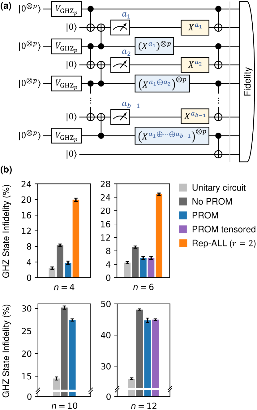
(a)

(b)

(c)

Figure 5: GHZ state preparation using feedforward. (a) Dynamic circuit to prepare an $n$-qubit GHZ state. The $n$ qubits are split into $b$ blocks each comprising $p$ qubits and an ancilla, the former prepared in a GHZ state through the standard unitary $\smash{V_{\textsc{ghz}_{p}}}$ comprising a fan-out of CX gates—see Figure S1b. Thereafter the small GHZ states are merged in constant depth through mid-circuit measurements and feedforward operations (shaded blue), and finally the ancillae are reset (shaded yellow) and absorbed into the state. (b) Infidelities of the prepared state against the ideal $n$-qubit GHZ state, comparing PROM, PROM assuming tensored readout channels, Rep-ALL at $r=2$, and without readout error mitigation for mid-circuit measurements and feedforward. Also shown are infidelities on a unitary circuit ($\smash{V_{\textsc{ghz}_{n}}}$). Readout error mitigation for terminal measurements was applied for all experiments. The $n=4,6,10,12$ experiments employed $(b,p)=(2,1)$, $(3,1)$, $(2,4)$, $(3,3)$ circuit structures respectively, executed on the superconducting quantum device ibm_osaka. Error bars are standard deviations across $100$ trials each with $10000$ shots.

Next we demonstrate PROM in the context of preparing GHZ states, which are entangled states of foundational importance across quantum information, metrology, and communications domains [79, 80, 81, 82]. On linear nearest-neighbor qubit connectivity, the unitary preparation of an $n$-qubit GHZ state ($n$ even) necessarily requires $n-1$ CX gates with $n/2$ depth [83]. The optimal unitary circuit comprises a qubit starting in the $\ket{+}$ state followed by a bidirectional fan-out of CX gates to grow the GHZ state (see Figure S1b).

With mid-circuit measurements and feedforward, however, a GHZ state can be prepared in constant depth independent of $n$ [84, 14, 83]. Here we examine a circuit structure that is an interpolation [84] between the unitary and feedforward circuit extremes (see Figure 5a), such that the number of CX gates and measurements in the circuit and circuit depth become adjustable. We consider splitting the $n$ qubits into $b$ blocks each containing $p$ system qubits and an ancillary qubit; smaller $p$-qubit GHZ states are unitarily prepared in each of the blocks, and the blocks are then merged in constant depth using mid-circuit measurements and feedforward. Conceptually, the ancillae perform parity checks on adjacent pairs of blocks, and detected domain walls in the quantum state are annihilated through feedforward (blue-shaded gates in Figure 5a). Lastly the ancillae are reset (yellow-shaded gates) and unitarily absorbed into the GHZ state. The constant-depth feedforward extreme discussed above corresponds to $(b,p)=(n/2,1)$. For $b\geq 2$, a $(b,p)$-circuit contains $b(p+2)-2$ CX gates, $b-1$ mid-circuit measurements, and is of depth $\lfloor p/2\rfloor+4$ including the layer of mid-circuit measurements on the ancillae.

First, we report results at $n=4,6$ in Figure 5b, using $(b,p)=(2,1),(3,1)$ circuit structures respectively. We compare the observed infidelity of the prepared state against the ideal GHZ state without PROM, with general PROM and PROM assuming tensored readout error channels, and with Rep-ALL at $r=2$. We include also for comparison the unitary GHZ state preparation circuit (drawn in Figure S1b) run on the same $n$-qubit chain. We used a stabilizer method to measure the fidelity of the prepared state against the GHZ state—see Sec. C.5 for details. The application of PROM is evidently effective, reducing state infidelities to ${\sim}45$–$65\%$ of their unmitigated values. Residual infidelities are attributed to quantum errors and decoherence that are not targeted by PROM. Just as in the qubit reset experiments (Sec. IV.1), the Rep-ALL mitigation scheme is not competitive.

The qualitative trend that unitary state preparation outperform unmitigated dynamic circuits is consistent with a prior study [14]; as discussed there and in other dynamic circuit studies [20], this is generally attributable to decoherence, crosstalk, and imperfect quantum-nondemolition (QND) properties of measurements on hardware. In our experiments, with PROM, the infidelities on dynamic circuits become fairly competitive with but do not surpass unitary circuits.

We next examined larger $n=10,12$ settings in Figure 5c, therein utilizing an interpolation between unitary and feedforward circuit extremes by choosing $(b,p)=(2,4),(3,3)$ circuit structures respectively. Here PROM provided reductions in state infidelities comparable to the $n=4,6$ experiments, but residual infidelities were expectedly higher. As it has become clear that the repetition-based REM schemes are uncompetitive, we have omitted them at $n=10,12$. On circuits with $b>2$, in particular $n=6,12$, general PROM yielded relative state infidelities ${\sim}1$–$2\%$ lower than PROM assuming independent readout errors—similar to the qubit reset experiments in Sec. IV.1, this small difference is consistent with our protocol sensitivity bounds as the characterized readout error channels were close to being independent.

We report additional data on a second superconducting quantum device in Sec. D.2.1 at $n=4,6$, which are qualitatively similar. There, we also report infidelities measured with Rep-ALL and Rep-MAJ at $r=3$, which were entirely uncompetitive and omitted here.

IV.3 Staged quantum state teleportation

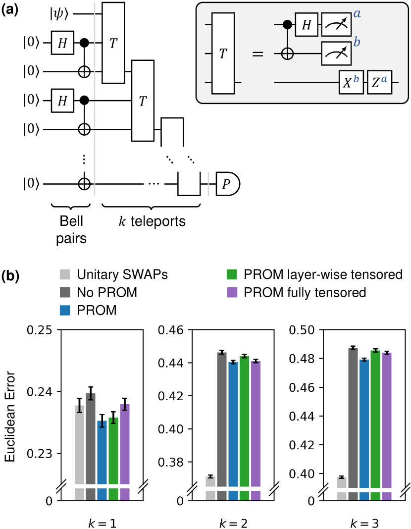
(a)

(b)

Figure 6: Repeated quantum state teleportation. (a) Circuit schematic. An input quantum state $\ket{\psi}$ is transported to a qubit a distance $2k$ away by $k$ teleportations, consuming $k$ shared Bell pairs. On the destination qubit, Pauli expectation values $\expectationvalue{P}$ are measured and the deviations $\delta P$ against ideal expectation values of the input state $\ket{\psi}$ assessed, for $P\in\{X,Y,Z\}$. (b) Euclidean errors $\smash{\Delta=(\delta X^{2}+\delta Y^{2}+\delta Z^{2})^{1/2}}$ after $k\in\{1,2,3\}$ teleportations, comparing PROM, PROM assuming layer-wise and fully tensored readout channels, and without readout error mitigation for mid-circuit measurements and feedforward. Also shown are errors on a unitary circuit with SWAP gates that transport $\ket{\psi}$ across the same qubits. Readout error mitigation for terminal measurements was applied for all cases. Experiments were performed on the superconducting quantum device ibm_osaka. Error bars are standard deviations across $100$ trials each with $1000000$ shots.

Lastly we investigate repeated quantum state teleportation (see Figure 6a). In standard state teleportation [85, 86, 87], a Bell pair is shared between a second and third qubit; the first qubit hosts the quantum state $\ket{\psi}$ to be transported. A Bell-basis measurement is performed on the first and second qubits and the outcomes feedforward into operations on the third qubit, which ends in state $\ket{\psi}$. As this procedure requires CX gates between adjacent pairs of qubits, the $3$ qubits must be connected to each other—thus $\ket{\psi}$ is transported a distance of $2$ qubits. Generically, repeating the teleportation $k$ times transports $\ket{\psi}$ a distance of $2k$ qubits (see Figure 6a). Scenarios that require the transport of a qubit state arise commonly in quantum computation and simulation, necessitated by device connectivity or classical control constraints [88, 89]. The straightforward alternative to teleportation is to connect starting and ending qubits with a path of SWAP gates, thus unitarily transporting the qubit state (see Figure S1c).

In our experiment, we prepare a generic single-qubit state $\smash{\ket{\psi}=e^{-i\phi_{z}Z}e^{-i\phi_{x}X}\ket{0}}$ with arbitrarily chosen $(\phi_{x},\phi_{z})=(\pi/8,3\pi/8)$, and teleport the state $k$ times, as drawn in Figure 6a. We terminally measure Pauli expectation values $\expectationvalue{X},\expectationvalue{Y},\expectationvalue{Z}$ on the ending qubit and assess their deviations $\delta X,\delta Y,\delta Z$ with respect to ideal values on the $\ket{\psi}$ starting state. To eliminate dependence on the measurement basis, we examine the Euclidean error $\smash{\Delta=(\delta X^{2}+\delta Y^{2}+\delta Z^{2})^{1/2}}$. Thus $\Delta$ provides an averaged measure of the degradation of the state $\ket{\psi}$ as it undergoes transport. We employ the multi-layer formulation of PROM, with each teleportation stage placed in a layer (totalling $k$ layers).

In Figure 6b we report results for $k\in\{1,2,3\}$ stages of teleportation, comparing the measured $\Delta$ without PROM, with general PROM, and with PROM assuming layer-wise and fully tensored readout error channels. We include also results on a unitary SWAP circuit transporting $\ket{\psi}$ across the same qubits. Across all $k$, PROM results in lower $\Delta$ than without mitigation. In particular at $k=1$ this improvement is sufficient for teleportation to be comparable in error to unitary SWAPs, but at higher $k$ the unitary circuit is better. Similar to prior experiments (Secs. IV.1 and IV.2), general PROM provides a relative advantage of ${\sim}1$–$2\%$ over PROM with independence assumptions, which is consistent with our sensitivity bounds.

We report additional data on a second quantum device in Sec. D.3.1, which are qualitatively similar. There we also show results with Rep-ALL at $r=2$, which were uncompetitive and omitted here.

V Discussion & Conclusion

In this work we have described a general readout error mitigation (REM) method targeting mid-circuit measurements and feedforward in dynamic circuits, for which existing standard techniques for terminal measurements cannot address. In addition to laying the theoretical groundwork, we demonstrated the effectiveness of our method in a series of experiments on superconducting quantum processors. These experiments spanned multiple use cases of practical interest with several performance measures—in each case the observed error metric significantly decreased with our REM method.

To accommodate arbitrary correlations in readout errors, the application of our REM protocol requires resources scaling exponentially with the number of measurements. This is a consequence of universal lower bounds on the cost of quantum error mitigation [90, 91, 92, 33], applied here to readout errors instead of error channels acting directly on the quantum state. However, under an assumption that readout errors are independent, a reduction of classical resources required to construct the mitigated estimator to polynomial (in fact linear) scaling can be achieved. On quantum devices exhibiting small error correlations this cheaper scheme can suffice in providing high-quality mitigation. The sensitivity and overhead bounds we provide could aid in identifying the variant of the mitigation protocol to utilize in an experiment.

Lastly, we remark that quantum error mitigation can in general be recast into the broader frameworks of quantum channel and resource distillation [93, 94, 95, 96]. The present REM context for feedforward is no exception. The probabilistic sampling to correct the effects of broken measurement-feedforward correlations here, for example, is reminiscent of the classical sampling to restore coherence in distillation protocols. We point out related ideas in recent works which demonstrated noise protection on a memory qubit [97] and considered building better positive operator-valued measures (POVMs) including accounting for quantum bit-flip errors during measurement [98]. Our protocol primarily targets readout errors on the measurement outcomes; however, we could also treat coherent errors using a combination of these techniques and our method, or by applying probabilistic error cancellation [38, 39].

Our study paves the way for effectively utilizing dynamic circuit capabilities on both near-term and future hardware. This supports pivotal quantum resource advantages across a broad range of domains and is imperative for realizing useful quantum computation.

Appendix A Preliminaries

A.1 Notation and basic facts

Throughout our work some symbols such as $s,t,f$ may represent a bitstring or bitvector when so defined. We do not distinguish between bitstrings and bitvectors. We use the following notation:

• The length of a bitstring $s$, that is, the number of bits in $s$, is denoted $\absolutevalue{s}$.

• The Hamming weight of a bitstring $s$, that is, the number of nonzero bits in $s$, is denoted $\operatorname*{wt}(s)$.

• The $j^{\text{th}}$-bit of a bitstring $s$ is denoted $s_{j}\in\{0,1\}$.

• The bit-wise sum, equivalently difference, of bitstrings $s$ and $t$ of equal length is $s\oplus t$, which is a bitstring.

• The dot product of bitstrings $s$ and $t$ of equal length is $\smash{s\cdot t=\sum_{j=1}^{\absolutevalue{s}}s_{j}t_{j}}\,\,(\text{mod}\,2)$, which is a bit.

• Where unambiguous by context, the concatenation of two bitstrings $s^{(1)}$ and $s^{(2)}$ is written simply $s^{(1)}s^{(2)}$.

• The all-zero bitstring is denoted $\mathbf{0}$, which has all entries zero. The all-one counterpart is denoted $\mathbf{1}$.

• Bitstrings can be used as indices. The basis for the vector, matrix or tensor is simply regarded as being enumerated (labelled) by the bitstrings. Alternatively one can implicitly convert the bitstrings to their decimal values for conventional integer enumeration.

We write $[n]=\{1,2,\ldots,n\}$ for $n\in\mathbb{N}$. We use the following notation for vectors, matrices and tensors:

• Vectors are written with boldface, for example $\mathbf{v}$. Matrices and tensors are not bolded, for example $A$.

• Entries are indexed with subscripts. For example $v_{j}$ is the $\smash{j^{\text{th}}}$ entry of a vector $\mathbf{v}$, and $A_{ij}$ is the $\smash{(i,j)^{\text{th}}}$ entry of a matrix $A$.

• $\smash{\norm{\mathbf{v}}}_{p}$ is the $p$-norm of a vector $\mathbf{v}$.

• $\smash{\norm{A}}_{p}$ for a matrix $A$ denotes the matrix norm induced by the vector $p$-norm. For example $\smash{\norm{A}}_{2}$ is the spectral norm of $A$ and is the largest singular value of $A$.

• $\absolutevalue{\mathbf{v}}$ and $\absolutevalue{A}$ are the entry-wise absolute values of a vector $\mathbf{v}$ and a matrix $A$, themselves a vector and a matrix respectively, not to be confused with the norms of $\mathbf{v}$ and $A$.

• $\mathbf{v}>\mathbf{v}^{\prime}$ means that $\mathbf{v}$ is entry-wise larger than $\mathbf{v}^{\prime}$, that is, $v_{j}>v^{\prime}_{j}$ for every index $j$. Likewise for $\geq,\leq,<$.

• The binary convolution between two vectors $\mathbf{u}$ and $\mathbf{v}$ of equal length is a vector with entries

  $$\begin{split}(\mathbf{u}\ast\mathbf{v})_{s}=\sum_{t\in\mathcal{S}}u_{t}v_{s\oplus t},\end{split}$$ (17)

  for each $s\in\mathcal{S}$, where $\mathcal{S}$ is the set of bitstrings indexing $\mathbf{u}$ and $\mathbf{v}$.

We use conventional notation for Pauli matrices and the Hadamard and $S$ gates,

$$\begin{split}X=\matrixquantity[0&1\\ 1&0],\qquad Y=\matrixquantity[0&-i\\ i&0],\qquad Z=\matrixquantity[1&0\\ 0&-1],\qquad H=\frac{1}{\sqrt{2}}\matrixquantity[1&1\\ 1&-1],\qquad S=\matrixquantity[1&0\\ 0&i],\end{split}$$ (18)

and the CX gate with the first qubit as control and the second qubit as target is written $\ket{0}\bra{0}\otimes\mathbb{I}+\ket{1}\bra{1}\otimes X$. We denote the identity as $\mathbb{I}$, with dimensions inferred from context. The $d$-fold tensor product of an object $A$, for instance quantum state, vector, or matrix, is denoted $A^{\otimes d}$. More generally we write

$$\begin{split}A^{(s)}=\bigotimes_{j=1}^{\absolutevalue{s}}A^{s_{j}},\end{split}$$ (19)

for a bitstring $s$, which is a $d$-fold tensor product over $\{A,\mathbb{I}\}$ as determined by the bitstring $s$. The diagonal entries of tensor products of $Z$ Pauli matrices (which are diagonal) satisfy

$$\begin{split}\left[Z^{(s)}\right]_{kk}=(-1)^{k\cdot s},\end{split}$$ (20)

where $k$ is a bitstring index. The entries of tensor products of $H$ satisfy

$$\begin{split}\sqrt{2^{m}}\left[H^{\otimes m}\right]_{fk}=\left[Z^{(f)}\right]_{kk}=(-1)^{f\cdot k},\end{split}$$ (21)

where $f$ and $k$ are bitstring indices.

A.2 Properties of confusion matrices $M$, $Q$ and vector $\mathbf{q}$

As written in Sec. I.1, in a setting with $m$ measurements, each entry $M_{ts}\in[0,1]$ records the probability of the quantum device reporting measurement outcome $t\in\mathcal{S}=\{0,1\}^{m}$ when the true outcome is $s\in\mathcal{S}$. Correspondingly $M$ is stochastic, i.e.

$$\begin{split}\sum_{t\in\mathcal{S}}M_{ts}=1\quad\forall\quad s\in\mathcal{S},\end{split}$$ (22)

and consequently,

$$\begin{split}\norm{M}_{1}=\max_{s\in\mathcal{S}}\underbrace{\sum_{t\in\mathcal{S}}\absolutevalue{M_{ts}}}_{1}=1.\end{split}$$ (23)

Each entry $q_{s}\in[0,1]$ of the symmetrized confusion vector $\mathbf{q}$, as in Sec. I.2, records the probability of a readout error syndrome $s\in\mathcal{S}$ occurring (with BFA applied)—that is, the probability that any true measurement outcome $a\in\mathcal{S}$ is reported as $a\oplus s$. This probability is uniform across $a\in\mathcal{S}$ due to the symmetrization of the readout channels. Correspondingly $\mathbf{q}$ is a probability distribution,

$$\begin{split}\sum_{s\in\mathcal{S}}q_{s}=1.\end{split}$$ (24)

The symmetrized confusion matrix $Q$ as in Sec. I.2, with entries $Q_{sf}=q_{s\oplus f}\in[0,1]$ for $s\in\mathcal{S}$ and $f\in\mathcal{S}$, is doubly stochastic, i.e.

$$\begin{split}\sum_{s\in\mathcal{S}}Q_{sf}&=\sum_{s\in\mathcal{S}}q_{s\oplus f}=\sum_{s^{\prime}\in\mathcal{S}}q_{s^{\prime}}=1\quad\forall\quad f\in\mathcal{S},\\ \sum_{f\in\mathcal{S}}Q_{sf}&=\sum_{f\in\mathcal{S}}q_{s\oplus f}=\sum_{s^{\prime}\in\mathcal{S}}q_{s^{\prime}}=1\quad\forall\quad s\in\mathcal{S},\end{split}$$ (25)

and consequently,

$$\begin{split}\norm{Q}_{1}&=\max_{f\in\mathcal{S}}\underbrace{\sum_{s\in\mathcal{S}}\absolutevalue{Q_{sf}}}_{1}=1,\qquad\norm{Q}_{\infty}=\max_{s\in\mathcal{S}}\underbrace{\sum_{f\in\mathcal{S}}\absolutevalue{Q_{sf}}}_{1}=1.\end{split}$$ (26)

For a more concrete visualization, below we give explicit forms of $Q$ for $m=1$, $m=2$ and $m=3$ cases,

$$\begin{split}Q=\matrixquantity[q_{0}&q_{1}\\ q_{1}&q_{0}],\qquad Q=\matrixquantity[q_{00}&q_{01}&q_{10}&q_{11}\\ q_{01}&q_{00}&q_{11}&q_{10}\\ q_{10}&q_{11}&q_{00}&q_{01}\\ q_{11}&q_{10}&q_{01}&q_{00}\\ ],\qquad Q=\matrixquantity[q_{000}&q_{001}&q_{010}&q_{011}&q_{100}&q_{101}&q_{110}&q_{111}\\ q_{001}&q_{000}&q_{011}&q_{010}&q_{101}&q_{100}&q_{111}&q_{110}\\ q_{010}&q_{011}&q_{000}&q_{001}&q_{110}&q_{111}&q_{100}&q_{101}\\ q_{011}&q_{010}&q_{001}&q_{000}&q_{111}&q_{110}&q_{101}&q_{100}\\ q_{100}&q_{101}&q_{110}&q_{111}&q_{000}&q_{001}&q_{010}&q_{011}\\ q_{101}&q_{100}&q_{111}&q_{110}&q_{001}&q_{000}&q_{011}&q_{010}\\ q_{110}&q_{111}&q_{100}&q_{101}&q_{010}&q_{011}&q_{000}&q_{001}\\ q_{111}&q_{110}&q_{101}&q_{100}&q_{011}&q_{010}&q_{001}&q_{000}\\ ].\end{split}$$ (27)

In an ideal setting without readout errors, $\smash{M_{ts}=\delta_{ts}}$ or equivalently $M=\mathbb{I}$ is the identity matrix. In the symmetrized picture, in the ideal setting the probability distribution $\mathbf{q}$ has support only on the trivial syndrome, $\smash{q_{s}=\delta_{s\mathbf{0}}}$, and correspondingly $Q=\mathbb{I}$ is the identity matrix.

In general, the following properties about the diagonal entries and trace of $Q$ hold,

$$\begin{split}Q_{ss}=q_{s\oplus s}=q_{\mathbf{0}}\quad\forall\quad s\in\mathcal{S},\qquad\qquad\tr Q=2^{m}q_{\mathbf{0}}.\end{split}$$ (28)

The determinant of $Q$ can also be analytically evaluated—see Eq. 36. This is most compactly done via the diagonalization of $Q$, which we describe in Sec. A.3.

Lastly, given an $M$, one can in fact compute the corresponding $\mathbf{q}$ and $Q$ that characterizes the symmetrized readout error channels, that would have been measured had BFA been used during calibration, and which would be needed for readout error mitigation in subsequent experiment circuits executed with BFA. In particular,

$$\begin{split}q_{s}=\frac{1}{2^{m}}\sum_{\begin{subarray}{c}t,t^{\prime}\in\mathcal{S}\\ t\oplus t^{\prime}=s\end{subarray}}M_{tt^{\prime}}=\frac{1}{2^{m}}\sum_{t\in\mathcal{S}}M_{t(t\oplus s)},\qquad Q_{sf}=q_{s\oplus f}=\frac{1}{2^{m}}\sum_{t\in\mathcal{S}}M_{t(t\oplus s\oplus f)},\end{split}$$ (29)

that is, $q_{s}$ is the average of all entries $M_{tt^{\prime}}$ consistent with the syndrome $t\oplus t^{\prime}=s$, and the construction of $Q$ follows from $\mathbf{q}$ by definition. The explicit meaning that $\mathbf{q}$ and $Q$ describe the readout error channels under symmetrization is thus made clear. We clarify, however, that in practice $\mathbf{q}$ and $Q$ can be directly obtained by including BFA in the calibration circuits, and there is no need to go through $M$. See Sec. C.2 for details on the calibration process as implemented in our experiments. This direct calibration with BFA provides resource and precision advantages [52, 53].

A.3 Diagonalization of symmetrized confusion matrix $Q$ and the inverse of $Q$

As noted in Sec. I.2 of the main text, $Q$ is hugely symmetric. Its entries $Q_{sf}$ are invariant under the index shift $(s,f)\to(s\oplus s^{\prime},f\oplus s^{\prime})$ for any $s^{\prime}\in\mathcal{S}$. In particular, $Q$ is symmetric about both its diagonal and anti-diagonal, and so is every of its recursively halved quadrants—see, for example, Eq. 27 for visualization. Recall that $m$-fold tensor products of the Pauli matrices form a basis for $2^{m}\times 2^{m}$ complex matrices, and of the Pauli matrices, only $\mathbb{I}$ and $X$ are symmetric about both their diagonal and anti-diagonal. Thus it follows that $Q$ must be of the form

$$\begin{split}Q=\sum_{s\in\mathcal{S}}A_{s}X^{(s)},\end{split}$$ (30)

for coefficients $A_{s}\in\mathbb{R}$, in order for it to possess the symmetries exhibited. To fix the coefficients, one examines the first column of $Q$, which must match $\mathbf{q}$ by definition. Note that the first column of $X^{(s)}$ has a unit entry at row $s$ and is zero everywhere else, $\smash{\big{[}X^{(s)}\big{]}_{r\mathbf{0}}=\delta_{rs}}$. Thus

$$\begin{split}Q_{r\mathbf{0}}=\sum_{s\in\mathcal{S}}A_{s}\left[X^{(s)}\right]_{r\mathbf{0}}=\sum_{s\in\mathcal{S}}A_{s}\delta_{rs}=A_{r}=q_{r}.\end{split}$$ (31)

That is,

$$\begin{split}Q=\sum_{s\in\mathcal{S}}q_{s}X^{(s)}.\end{split}$$ (32)

Now note that $X^{(s)}$ is diagonalized by $H^{\otimes m}$, that is, $H^{\otimes m}X^{(s)}H^{\otimes m}=Z^{(s)}$. Then $Q$, which is a linear combination of $X^{(s)}$, is also diagonalized by $H^{\otimes m}$,

$$\begin{split}H^{\otimes m}QH^{\otimes m}=\sum_{s\in\mathcal{S}}q_{s}Z^{(s)}.\end{split}$$ (33)

The eigenvalues of $Q$ are thus given by

$$\begin{split}\lambda_{k}=\sum_{s\in\mathcal{S}}q_{s}\left[Z^{(s)}\right]_{kk}=\sum_{s\in\mathcal{S}}(-1)^{k\cdot s}q_{s},\end{split}$$ (34)

where we have invoked the identity in Eq. 20. Recalling the normalization $\sum_{s\in\mathcal{S}}q_{s}=1$, one can obtain an alternate form

$$\begin{split}\lambda_{k}=q_{\mathbf{0}}+\sum_{\begin{subarray}{c}s\in\mathcal{S}\\ s\neq\mathbf{0}\end{subarray}}(-1)^{k\cdot s}q_{s}=\left(1-\sum_{\begin{subarray}{c}s\in\mathcal{S}\\ s\neq\mathbf{0}\end{subarray}}q_{s}\right)+\sum_{\begin{subarray}{c}s\in\mathcal{S}\\ s\neq\mathbf{0}\end{subarray}}(-1)^{k\cdot s}q_{s}&=1-\sum_{\begin{subarray}{c}s\in\mathcal{S}\\ s\neq\mathbf{0}\end{subarray}}\left[1-(-1)^{k\cdot s}\right]q_{s}\\ &=1-2\sum_{\begin{subarray}{c}s\in\mathcal{S}\\ k\cdot s\neq 0\end{subarray}}q_{s},\end{split}$$ (35)

which makes the special case $\lambda_{\mathbf{0}}=1$ clear. The solutions for the eigenvalues in $Q$ in Eqs. 34 and 35 above are reported in Eq. 3 of the main text. In general, as $Q$ is doubly stochastic, as in Eq. 25, we are guaranteed that $\absolutevalue{\lambda_{k}}\leq 1$ for all $k\in\mathcal{S}$. In the absence of readout errors ($\smash{q_{s}=\delta_{s\mathbf{0}}}$), we straightforwardly have ${\bf\it\lambda}=\mathbf{1}$, that is, $\lambda_{k}=1$ uniformly for all $k\in\mathcal{S}$. Lastly we comment that the trace and determinant of $Q$ yield the properties

$$\begin{split}\tr Q&=\sum_{k\in\mathcal{S}}\lambda_{k}=2^{m}q_{\mathbf{0}},\\ \det Q&=\prod_{k\in\mathcal{S}}\lambda_{k}=\prod_{k\in\mathcal{S}}\left[\sum_{s\in\mathcal{S}}(-1)^{k\cdot s}q_{s}\right]=\prod_{k\in\mathcal{S}}\left[1-2\sum_{\begin{subarray}{c}s\in\mathcal{S}\\ k\cdot s\neq 0\end{subarray}}q_{s}\right],\end{split}$$ (36)

where in the first line we have used our prior result for the trace of $Q$ in Eq. 28. As $Q$ is stochastic we have that $\absolutevalue{\det Q}\leq 1$, and Eq. 36 implies $\absolutevalue{\det Q}=1$ only when no readout errors are present.

In anticipation of developments in Appendix B, we examine $Q^{-1}$. Trivially, we remind that in an ideal setting without readout errors, $Q=\mathbb{I}$ and thus $Q^{-1}=\mathbb{I}$. Now, the diagonalization of $Q$ from Eq. 33 gives

$$\begin{split}Q^{-1}=H^{\otimes m}\matrixquantity[\frac{1}{\lambda_{1}}&&&\\ &\frac{1}{\lambda_{2}}&&\\ &&\ddots&\\ &&&\frac{1}{\lambda_{m}}]H^{\otimes m},\end{split}$$ (37)

and thus entries of $Q^{-1}$ can be written as

$$\begin{split}\left[Q^{-1}\right]_{sf}&=\sum_{k\in\mathcal{S}}\left[H^{\otimes m}\right]_{sk}\left(\frac{1}{\lambda_{k}}\right)\left[H^{\otimes m}\right]_{kf}\\ &=\frac{1}{2^{m}}\sum_{k\in\mathcal{S}}(-1)^{s\cdot k}(-1)^{k\cdot f}\left(\frac{1}{\lambda_{k}}\right),\end{split}$$ (38)

where we have used the identities for entries of tensor products of $H$ matrices in Eq. 21. For future use, we note that the first column of $Q^{-1}$ is given by

$$\begin{split}\left[Q^{-1}\right]_{s\mathbf{0}}=\frac{1}{2^{m}}\sum_{k\in\mathcal{S}}(-1)^{s\cdot k}\left(\frac{1}{\lambda_{k}}\right).\end{split}$$ (39)

Moreover, that $Q$ is hugely symmetric implies the same for $Q^{-1}$—namely, that the entries $[Q^{-1}]_{sf}$ are invariant under the index shift $(s,f)\to(s\oplus s^{\prime},f\oplus s^{\prime})$ for any $s^{\prime}\in\mathcal{S}$, indeed also explicitly observable in Eq. 38. In particular, we observe $\smash{[Q^{-1}]_{sf}=[Q^{-1}]_{(s\oplus f)\mathbf{0}}=[Q^{-1}]_{\mathbf{0}(s\oplus f)}}$, and thus each column and row of $Q^{-1}$ contains the same entries but arranged in different orders. This means

$$\begin{split}\norm{Q^{-1}}_{1}&=\max_{f\in\mathcal{S}}\sum_{s\in\mathcal{S}}\absolutevalue{[Q^{-1}]_{sf}}=\sum_{s\in\mathcal{S}}\absolutevalue{[Q^{-1}]_{s\mathbf{0}}},\\ \norm{Q^{-1}}_{\infty}&=\max_{s\in\mathcal{S}}\sum_{f\in\mathcal{S}}\absolutevalue{[Q^{-1}]_{sf}}=\sum_{f\in\mathcal{S}}\absolutevalue{[Q^{-1}]_{\mathbf{0}f}}.\end{split}$$ (40)

Also, from $QQ^{-1}=Q^{-1}Q=\mathbb{I}$, we observe that row and column sums of $Q^{-1}$ evaluate uniformly to unity,

$$\begin{split}\sum_{k\in\mathcal{S}}Q_{sk}[Q^{-1}]_{kf}=\delta_{sf}&\Longrightarrow\sum_{s\in\mathcal{S}}\sum_{k\in\mathcal{S}}Q_{sk}[Q^{-1}]_{kf}=\sum_{k\in\mathcal{S}}\underbrace{\left(\sum_{s\in\mathcal{S}}Q_{sk}\right)}_{1}[Q^{-1}]_{kf}=\sum_{k\in\mathcal{S}}[Q^{-1}]_{kf}=\sum_{s\in\mathcal{S}}\delta_{sf}=1\quad\forall\quad f\in\mathcal{S},\\ \sum_{k\in\mathcal{S}}[Q^{-1}]_{sk}Q_{kf}=\delta_{sf}&\Longrightarrow\sum_{f\in\mathcal{S}}\sum_{k\in\mathcal{S}}[Q^{-1}]_{sk}Q_{kf}=\sum_{k\in\mathcal{S}}[Q^{-1}]_{sk}\underbrace{\left(\sum_{f\in\mathcal{S}}Q_{kf}\right)}_{1}=\sum_{k\in\mathcal{S}}[Q^{-1}]_{sk}=\sum_{f\in\mathcal{S}}\delta_{sf}=1\quad\forall\quad s\in\mathcal{S},\end{split}$$ (41)

where we have used the fact that $Q$ is doubly stochastic, as in Eq. 25. Despite this property, we clarify that $Q^{-1}$ is not generally doubly stochastic as its entries are not guaranteed to be non-negative. In fact $QQ^{-1}=Q^{-1}Q=\mathbb{I}$ implies that each row and column of $Q^{-1}$ must contain at least one negative entry when readout errors are present (when $Q\neq\mathbb{I}$).

A.4 Tensored readout channels

A.4.1 General setting

Consider a setting wherein we partition the $m$ measurements into subsets of sizes $\smash{\{m^{(1)},m^{(2)},\ldots,m^{(p)}\}}$, where $\smash{m^{(\ell)}\geq 1}$ for each $\ell$ and $\smash{m^{(1)}+m^{(2)}+\cdots+m^{(p)}=m}$, and we make the assumption that there are no correlations in readout errors between measurements in different subsets. That is, readout errors in different subsets are independent; but within a subset correlations in readout error can be present. One then has the decomposition

$$\begin{split}M=\bigotimes_{\ell=1}^{p}M^{(\ell)},\end{split}$$ (42)

where $\smash{M^{(\ell)}}$ is a $\smash{2^{m^{(\ell)}}\times 2^{m^{(\ell)}}}$-sized confusion matrix characterizing readout errors affecting the $\ell^{\text{th}}$ subset of measurements. This is equivalent to a statement of factorization of probabilities

$$\begin{split}M_{ts}=\prod_{\ell=1}^{p}M^{(\ell)}_{t^{(\ell)}s^{(\ell)}},\end{split}$$ (43)

where $\smash{s=s^{(1)}s^{(2)}\ldots s^{(p)}\in\mathcal{S}}$ and $\smash{t=t^{(1)}t^{(2)}\ldots t^{(p)}\in\mathcal{S}}$ are the corresponding partitionings of the bitstrings over the $p$ subsets, $\smash{s^{(\ell)}\in\{0,1\}^{m^{(\ell)}}}$ and $\smash{t^{(\ell)}\in\{0,1\}^{m{(\ell)}}}$ for each $\ell\in[p]$. Likewise,

$$\begin{split}\mathbf{q}&=\bigotimes_{\ell=1}^{p}\mathbf{q}^{(\ell)},\qquad q_{s}=\prod_{\ell=1}^{p}q^{(\ell)}_{s^{(\ell)}},\\ Q&=\bigotimes_{\ell=1}^{p}Q^{(\ell)},\qquad Q_{sf}=\prod_{\ell=1}^{p}Q^{(\ell)}_{s^{(\ell)}f^{(\ell)}},\end{split}$$ (44)

with $\smash{s=s^{(1)}s^{(2)}\ldots s^{(p)}\in\mathcal{S}}$ and $\smash{f=f^{(1)}f^{(2)}\ldots f^{(p)}\in\mathcal{S}}$ being partitionings of the bitstrings, and where $\smash{\mathbf{q}^{(\ell)}}$ is a $\smash{2^{m^{(\ell)}}}$-length probability vector and $\smash{Q^{(\ell)}}$ is the corresponding $\smash{2^{m^{(\ell)}}\times 2^{m^{(\ell)}}}$-sized symmetrized confusion matrix characterizing readout errors affecting the $\ell^{\text{th}}$ subset of measurements. It follows from this tensor product structure that the eigenvalues of $Q$ factorize,

$$\begin{split}{\bf\it\lambda}=\bigotimes_{\ell=1}^{p}{\bf\it\lambda}^{(\ell)},\qquad\lambda_{k}=\prod_{\ell=1}^{m}\lambda^{(\ell)}_{k^{(\ell)}},\end{split}$$ (45)

where $\smash{{\bf\it\lambda}^{(\ell)}}$ are the eigenvalues of $Q^{(\ell)}$ and are given by the same solutions as in Eqs. 34 and 35, but with $\mathbf{q}^{(\ell)}$ taking the place of $\mathbf{q}$. Likewise the inverse of $Q$ factorizes,

$$\begin{split}Q^{-1}=\bigotimes_{\ell=1}^{p}Q^{(\ell)^{-1}},\qquad\left[Q^{-1}\right]_{sf}=\prod_{\ell=1}^{p}\left[Q^{(\ell)^{-1}}\right]_{s^{(\ell)}f^{(\ell)}},\qquad\left[Q^{-1}\right]_{s\mathbf{0}}=\prod_{\ell=1}^{p}\left[Q^{(\ell)^{-1}}\right]_{s^{(\ell)}\mathbf{0}},\end{split}$$ (46)

where $\smash{Q^{(\ell)^{-1}}}$ is the inverse of $Q^{(\ell)}$, whose general and first-column entries are given in Eq. 38 and Eq. 39, but now with ${\bf\it\lambda}^{(\ell)}$ taking the place of $\mathbf{\lambda}$.

A.4.2 Layer-wise tensored readout channels

In a feedforward circuit with $L>1$ layers (i.e. the setting of Sec. III of the main text), the discussion above straightforwardly applies when an assumption of layer-wise independence of readout errors is made. That is, readout errors on measurements in different layers of the circuit are taken to be independent, but we accommodate arbitrary correlations between errors in the same layer. Then in the notation of Sec. A.4.1 above, one takes $p=L$, and the subsets correspond to the measurements in each layer, $\smash{\{m^{[1]},m^{[2]},\ldots,m^{[L]}\}}$. The factorization of $\mathbf{q}$, $Q$, $Q^{-1}$ and eigenvalues ${\bf\it\lambda}$ then follow. In this setting we use square brackets for superscripts, for example $\mathbf{q}^{[l]}$ instead of $\mathbf{q}^{(l)}$, to emphasize the physical meaning that the indices enumerate the layers of the feedforward circuit, as is consistent with our writing in the main text.

A.4.3 Fully tensored readout channels

The setup in Sec. A.4.1 likewise applies in a setting where every measurement is assumed to be independent—then $p=m$ and the subsets $\smash{\{m^{(1)},m^{(2)},\ldots,m^{(p)}\}}$ are single measurements. To be explicit, in the factorization of $M$ in Eq. 42, we have in this setting

$$\begin{split}M^{(\ell)}=\matrixquantity[1-M^{(\ell)}_{10}&M^{(\ell)}_{01}\\ M^{(\ell)}_{10}&1-M^{(\ell)}_{01}],\end{split}$$ (47)

which are $2\times 2$ confusion matrices each characterizing the readout error affecting the $\ell$-th measurement, for $\ell\in[m]$. The diagonal elements record the probabilities of $0$ and $1$ outcomes being correctly reported, whereas off-diagonals record probabilities of bit-flip errors. With symmetrization, one has

$$\begin{split}\mathbf{q}^{(\ell)}=\matrixquantity[1-r_{\ell}\\ r_{\ell}],\end{split}$$ (48)

where $r_{\ell}$ is the probability of a readout error occurring on the $\ell$-th measurement. Concretely, the symmetrization means that $\smash{r_{\ell}=(M^{(\ell)}_{01}+M^{(\ell)}_{10})/2}$, which is expressed more generally in Eq. 29. Likewise, the symmetrized confusion matrices

$$\begin{split}Q^{(\ell)}=\matrixquantity[q^{(\ell)}_{0}&q^{(\ell)}_{1}\\ q^{(\ell)}_{1}&q^{(\ell)}_{0}]=\matrixquantity[1-r_{\ell}&r_{\ell}\\ r_{\ell}&1-r_{\ell}],\end{split}$$ (49)

whose diagonal and off-diagonals elements record probabilities of the measurement outcome being correctly and incorrectly reported respectively. The eigenvalues of $\smash{Q^{(\ell)}}$ are easily found to be

$$\begin{split}{\bf\it\lambda}^{(\ell)}=\matrixquantity[1\\ 1-2r_{\ell}],\end{split}$$ (50)

which coincides with our general solution for $\lambda_{k}$ in Eqs. 34 and 35 or Eq. 3 of the main text, setting $m=1$ for a single independent qubit. The inverse of $\smash{Q^{(\ell)}}$ is also easily found,

$$\begin{split}Q^{(\ell)^{-1}}=\frac{1}{1-2r_{\ell}}\matrixquantity[1-r_{\ell}&-r_{\ell}\\ -r_{\ell}&1-r_{\ell}],\end{split}$$ (51)

which is consistent with the general solution for entries of $Q^{-1}$ in Eq. 38 upon substitution of the present setting.

Appendix B Further Technical Details on Probabilistic Readout Error Mitigation

B.1 Theory for a single feedforward layer

B.1.1 General solution of ${\bf\it\alpha}$ for arbitrarily correlated readout channels

Here we provide an elaboration of the derivation in Sec. II.2 of the main text, leading to the general solution for ${\bf\it\alpha}$ in Eq. 10. First, in the absence of readout errors, the quantum state after the mid-circuit measurements and feedforward is straightforwardly

$$\begin{split}\overline{\sigma}=\sum_{s\in\mathcal{S}}V_{s}\Pi_{s}\rho\Pi_{s}V_{s}^{\dagger},\end{split}$$ (52)

where $\Pi_{s}$ is the measurement projector associated with the outcome $s\in\mathcal{S}$. Equivalently, in the picture of quantum trajectories,

$$\begin{split}\overline{\sigma}=\sum_{s\in\mathcal{S}}p_{s}V_{s}\rho_{s}V_{s}^{\dagger},\qquad\rho_{s}=\frac{\Pi_{s}\rho\Pi_{s}}{p_{s}},\qquad p_{s}=\tr\left(\Pi_{s}\rho\right),\end{split}$$ (53)

which was presented in Eq. 5 of the main text. Technically, here $\rho_{s}$ is well-defined so long as $p_{s}\neq 0$; the $p_{s}=0$ trajectories are immaterial to $\smash{\overline{\sigma}}$ and can be disregarded. In the presence of readout errors characterized by $\mathbf{q}$, and imposing a bitmask $f\in\mathcal{S}$ in feedforward, the quantum state after the mid-circuit measurements and feedforward is

$$\begin{split}\sigma^{(f)}=\sum_{s\in\mathcal{S}}\sum_{s^{\prime}\in\mathcal{S}}q_{s\oplus s^{\prime}}V_{s^{\prime}\oplus f}\Pi_{s}\rho\Pi_{s}V_{s^{\prime}\oplus f}^{\dagger}=\sum_{s\in\mathcal{S}}\sum_{s^{\prime}\in\mathcal{S}}q_{s\oplus s^{\prime}}p_{s}V_{s^{\prime}\oplus f}\rho_{s}V_{s^{\prime}\oplus f}^{\dagger},\end{split}$$ (54)

where the second equality was presented in Eq. 8 of the main text. The definition of the tensor $T$ follows,

$$\begin{split}T_{bss^{\prime}}=\tr\left(O_{b}V_{s^{\prime}}\Pi_{s}\rho\Pi_{s}V_{s^{\prime}}^{\dagger}\right)=p_{s}\tr\left(O_{b}V_{s^{\prime}}\rho_{s}V_{s^{\prime}}^{\dagger}\right),\end{split}$$ (55)

as presented in Eq. 6 of the main text. Then from Eq. 7, one has

$$\begin{split}\expectationvalue{\overline{O}_{b}}=\tr T_{b}=\sum_{s\in\mathcal{S}}T_{bss}=\sum_{s\in\mathcal{S}}\sum_{s^{\prime}\in\mathcal{S}}\delta_{ss^{\prime}}T_{bss}.\end{split}$$ (56)

At the same time, from Eq. 9,

$$\begin{split}\expectationvalue{O_{b}^{(f)}}=\sum_{s\in\mathcal{S}}\sum_{s^{\prime}\in\mathcal{S}}q_{s\oplus s^{\prime}}T_{bs(s^{\prime}\oplus f)}=\sum_{s\in\mathcal{S}}\sum_{s^{\prime}\in\mathcal{S}}q_{s\oplus s^{\prime}\oplus f}T_{bss^{\prime}}.\end{split}$$ (57)

Thus, by the definition of $\widehat{\mathbf{O}}$ in Eq. 4,

$$\begin{split}\expectationvalue*{\widehat{O}_{b}}=\sum_{f\in\mathcal{S}}\alpha_{f}\expectationvalue{O_{b}^{(f)}}=\sum_{f\in\mathcal{S}}\sum_{s\in\mathcal{S}}\sum_{s^{\prime}\in\mathcal{S}}\alpha_{f}q_{s\oplus s^{\prime}\oplus f}T_{bss^{\prime}}.\end{split}$$ (58)

We desire $\smash{\expectationvalue*{\widehat{\mathbf{O}}}=\expectationvalue*{\overline{\mathbf{O}}}}$ independent of the tensor $T$, which is unknown to us. This guarantees that the mitigation protocol works for arbitrary quantum circuits of the structure considered, with no additional problem-specific information required. The equality necessitates that the coefficients of every $T_{bss^{\prime}}$ match on both sides, in particular, between Eq. 56 and Eq. 58 for every $b\in[B]$, yielding

$$\begin{split}\sum_{f\in\mathcal{S}}\alpha_{f}q_{s\oplus s^{\prime}\oplus f}=\delta_{ss^{\prime}}\quad\forall\quad s,s^{\prime}\in\mathcal{S}.\end{split}$$ (59)

Noting that $\delta_{ss^{\prime}}=\delta_{(s\oplus s^{\prime})\mathbf{0}}$, the above reduces to

$$\begin{split}\sum_{f\in\mathcal{S}}\alpha_{f}q_{s\oplus f}=\delta_{s\mathbf{0}}\quad\forall\quad s\in\mathcal{S}.\end{split}$$ (60)

This linear system can be written as

$$\begin{split}Q{\bf\it\alpha}=\matrixquantity[1\\ 0\\ \vdots\\ 0]\Longleftrightarrow{\bf\it\alpha}=Q^{-1}\matrixquantity[1\\ 0\\ \vdots\\ 0].\end{split}$$ (61)

That is, ${\bf\it\alpha}$ is the first column of $Q^{-1}$. Then by Eq. 39, we have

$$\begin{split}\alpha_{f}=\left[Q^{-1}\right]_{f\mathbf{0}}=\frac{1}{2^{m}}\sum_{k\in\mathcal{S}}(-1)^{f\cdot k}\left(\frac{1}{\lambda_{k}}\right),\end{split}$$ (62)

which is the solution reported in Eq. 10 of the main text. This exactly coincides with and can be equivalently written as ${\bf\it\alpha}=\mathcal{W}(\mathbf{1}/{\bf\it\lambda})/2^{m}$ for $\mathcal{W}$ the unnormalized Walsh-Hadamard transform [60, 61], as also reported in the main text. Noting that $\lambda_{\mathbf{0}}=1$, as discussed in Sec. A.3, we obtain also the alternate expression

$$\begin{split}\alpha_{f}=\frac{1}{2^{m}}\left[\frac{1}{\lambda_{\mathbf{0}}}+\sum_{\begin{subarray}{c}k\in\mathcal{S}\\ k\neq\mathbf{0}\end{subarray}}(-1)^{f\cdot k}\left(\frac{1}{\lambda_{k}}\right)\right]=\frac{1}{2^{m}}\left[1+\sum_{\begin{subarray}{c}k\in\mathcal{S}\\ k\neq\mathbf{0}\end{subarray}}(-1)^{f\cdot k}\left(\frac{1}{\lambda_{k}}\right)\right].\end{split}$$ (63)

For illustration, in Table S1 we provide explicitly written solutions for ${\bf\it\alpha}$ at small $m$. For brevity we have used the form of ${\bf\it\alpha}$ in Eq. 63, and the form of ${\bf\it\lambda}$ in Eq. 35.

$m$	Solution
$1$	$\begin{aligned} \alpha_{0}&=\frac{1}{2}\left(1+\frac{1}{1-2q_{1}}\right)&\\ \alpha_{1}&=\frac{1}{2}\left(1-\frac{1}{1-2q_{1}}\right)\end{aligned}$
$2$	$\begin{aligned} \alpha_{00}&=\frac{1}{4}\left(1+\frac{1}{1-2q_{01}-2q_{10}}+\frac{1}{1-2q_{01}-2q_{11}}+\frac{1}{1-2q_{10}-2q_{11}}\right)&\\ \alpha_{01}&=\frac{1}{4}\left(1-\frac{1}{1-2q_{01}-2q_{10}}-\frac{1}{1-2q_{01}-2q_{11}}+\frac{1}{1-2q_{10}-2q_{11}}\right)&\\ \alpha_{10}&=\frac{1}{4}\left(1-\frac{1}{1-2q_{01}-2q_{10}}+\frac{1}{1-2q_{01}-2q_{11}}-\frac{1}{1-2q_{10}-2q_{11}}\right)&\\ \alpha_{11}&=\frac{1}{4}\left(1+\frac{1}{1-2q_{01}-2q_{10}}-\frac{1}{1-2q_{01}-2q_{11}}-\frac{1}{1-2q_{10}-2q_{11}}\right)&\\ \end{aligned}$
$3$	$\begin{aligned} \alpha_{000}=\frac{1}{8}\bigg{(}1&+\frac{1}{1-2q_{010}-2q_{011}-2q_{100}-2q_{101}}+\frac{1}{1-2q_{001}-2q_{011}-2q_{100}-2q_{110}}\\ &+\frac{1}{1-2q_{001}-2q_{010}-2q_{101}-2q_{110}}+\frac{1}{1-2q_{001}-2q_{010}-2q_{100}-2q_{111}}\\ &+\frac{1}{1-2q_{001}-2q_{011}-2q_{101}-2q_{111}}+\frac{1}{1-2q_{010}-2q_{011}-2q_{110}-2q_{111}}\\ &+\frac{1}{1-2q_{100}-2q_{101}-2q_{110}-2q_{111}}\bigg{)}&\\ \alpha_{001}=\frac{1}{8}\bigg{(}1&-\ldots\bigg{)}&\\ \end{aligned}$

Table S1: Explicitly written general solutions for ${\bf\it\alpha}$ at small $m$ for illustrative purposes. In consideration of space and readability, $\alpha_{k}$ entries for $m=3$ and $k\neq\mathbf{0}$ are left out; they follow the same form as $\alpha_{\mathbf{0}}$ but with sign flips on individual terms.

Resource complexity. In this general setting, a naïve procedure of obtaining ${\bf\it\alpha}$ is first to compute ${\bf\it\lambda}$ from $\mathbf{q}$ using Eq. 34 or Eq. 35, which comprises $2^{m}$ entries each involving a sum over extensively many entries of $\mathbf{q}$. Then ${\bf\it\alpha}$ is computed from ${\bf\it\lambda}$ using Eq. 62 or Eq. 63. Each of these steps require $\smash{\order{2^{2m}}}$ time and $\smash{\order{2^{m}}}$ space in classical resources, for the same overall complexity. But noting that $\mathbf{q}$, ${\bf\it\lambda}$ and ${\bf\it\alpha}$ are related by Walsh-Hadamard transforms, as noted in the main text and in the discussion above, one can in fact utilize the fast Walsh–Hadamard transform (FWHT) algorithm [99, 61], which runs in $\order{N\log N}$ time and $\order{N}$ space for an $N$-length input vector, for a more efficient solution computation procedure. This reduces the time complexity of solution computation to $\order{m\cdot 2^{m}}$ and maintains space complexity at $\order{2^{m}}$. Explicitly, the procedure goes as follows:

1. Perform unnormalized FWHT to compute ${\bf\it\lambda}=\mathcal{W}(\mathbf{q})$, requiring $\order{m\cdot 2^{m}}$ time and $\order{2^{m}}$ space.

2. Compute in-place element-wise division $\mathbf{1}/{\bf\it\lambda}$, requiring $\order{2^{m}}$ time.

3. Perform unnormalized FWHT to compute ${\bf\it\alpha}=\mathcal{W}(\mathbf{1}/{\bf\it\lambda})/2^{m}$, requiring $\order{m\cdot 2^{m}}$ time and $\order{2^{m}}$ space.

Thereafter, computing $\xi$ and $\absolutevalue{{\bf\it\alpha}}/\xi$ take sub-dominant $\order{2^{m}}$ time, the latter doable in-place. Lastly, standard algorithms to sample from an explicit probability distribution, such as alias and table methods [100, 64, 63, 62], allow the drawing of bitmasks $f\in\mathcal{S}$ from the distribution $\absolutevalue{{\bf\it\alpha}}/\xi$ in $\order{1}$ time per shot, with an initial pre-processing time linear in the number of entries in the distribution, a sub-dominant $\order{2^{m}}$ in the context here. The overall resource requirements of $\smash{\order{m\cdot 2^{m}}}$ time and $\smash{\order{2^{m}}}$ space for solution computation and $\order{1}$ time per shot are reported in Table 1 of the main text.

B.1.2 Simplified solution of ${\bf\it\alpha}$ for tensored readout channels

As outlined in Sec. II.3, making an assumption that readout errors on each of the $m$ measurements are independent, equivalently that the readout error channel acting on the $m$ measurements factorizes into a tensor product of channels acting on individual measurements, allows a simplification of the ${\bf\it\alpha}$ solution. In particular, under such a setting, $\mathbf{q}$, $Q$ and $Q^{-1}$ each factorizes into a tensor product of single-measurement counterparts, as worked through in Sec. A.4.3. Then from Eqs. 46 and 51, we have

$$\begin{split}{\bf\it\alpha}=\bigotimes_{\ell=1}^{m}{\bf\it\alpha}^{(\ell)},\qquad{\bf\it\alpha}^{(\ell)}=\frac{1}{1-2r_{\ell}}\matrixquantity[1-r_{\ell}\\ -r_{\ell}],\end{split}$$ (64)

where $\smash{{\bf\it\alpha}^{(\ell)}}$ are coefficients for the $\ell$-measurement. This is presented as Eq. 12 in the main text. Equivalently,

$$\begin{split}\alpha_{f}=\prod_{\ell=1}^{m}\alpha^{(\ell)}_{f_{\ell}},\qquad\alpha^{(\ell)}_{b}=\frac{r_{\ell}^{b}(r_{\ell}-1)^{1-b}}{2r_{\ell}-1},\end{split}$$ (65)

where $b\in\{0,1\}$. The overhead factor associated with mitigating the $\ell$-measurement is easily computed,

$$\begin{split}\xi^{(\ell)}=\norm{{\bf\it\alpha}^{(\ell)}}_{1}=\frac{1}{1-2r_{\ell}},\end{split}$$ (66)

and Eq. 64 implies that

$$\begin{split}\xi=\norm{{\bf\it\alpha}}_{1}=\prod_{\ell=1}^{m}\norm{{\bf\it\alpha}^{(\ell)}}_{1}=\prod_{\ell=1}^{m}\xi^{(\ell)}=\prod_{\ell=1}^{m}\frac{1}{1-2r_{\ell}},\end{split}$$ (67)

which is presented as Eq. 13 of the main text.

Resource complexity. The product structure of ${\bf\it\alpha}$ and $\xi$ above imply that $\absolutevalue{{\bf\it\alpha}}/\xi$ is a product over the individual $\absolutevalue{{\bf\it\alpha}^{(\ell)}}/\xi^{(\ell)}$ probability distributions,

$$\begin{split}\frac{\absolutevalue{{\bf\it\alpha}}}{\xi}=\bigotimes_{\ell=1}^{m}\frac{\absolutevalue{{\bf\it\alpha}^{(\ell)}}}{\xi^{(\ell)}}\Longleftrightarrow\frac{\absolutevalue{\alpha_{f}}}{\xi}=\prod_{\ell=1}^{m}\frac{\absolutevalue{\alpha^{(\ell)}_{f_{\ell}}}}{\xi^{(\ell)}}.\end{split}$$ (68)

The probability distributions $\smash{\absolutevalue{{\bf\it\alpha}^{(\ell)}}/\xi^{(\ell)}}$ and overall rescaling factor $\xi$ to be applied at the end of the mitigation protocol can be computed in $\order{m}$ time and space, as there are $2m$ entries across all $\smash{{\bf\it\alpha}^{(\ell)}}$ and $m$ overhead factors $\smash{\xi^{(\ell)}}$ in total, as explicitly written above. Then, for each experiment shot, a round of sampling can be used to draw $f_{\ell}$ from the distribution $\smash{\absolutevalue{{\bf\it\alpha}^{(\ell)}}/\xi^{(\ell)}}$ for each $\ell\in[m]$, thus producing a bitmask $f\in\mathcal{S}$ from the product distribution $\smash{\absolutevalue{{\bf\it\alpha}}/\xi}$ in $\order{m}$ time. These complexities are reflected in Table 1 of the main text.

In the simpler setting of uniform readout channels, $r_{\ell}=r$ for all $\ell\in[m]$ and all the $\smash{\absolutevalue{{\bf\it\alpha}^{(\ell)}}/\xi^{(\ell)}}$ distributions are identical. Thus, one needs to only compute a single $\smash{\absolutevalue{{\bf\it\alpha}^{(\ell)}}/\xi^{(\ell)}}$, which requires $\order{1}$ space and time. Then, for each experiment shot, $m$ rounds of sampling can be used to draw $f_{\ell}$ from the $\smash{\absolutevalue{{\bf\it\alpha}^{(\ell)}}/\xi^{(\ell)}}$ distribution repeatedly, thus building up the bitmask $f\in\mathcal{S}$ for the shot in $\order{m}$ time. This is also reflected in Table 1 of the main text.

B.2 Multiple feedforward layers

B.2.1 General solution of ${\bf\it\alpha}$ for arbitrarily correlated readout channels

Similar to Sec. B.1.1, here we provide an elaboration of the discussion in Sec. III.2 of the main text. To start, we write the quantum state after the $L$ layers of mid-circuit measurements and feedforward in the absence of readout errors,

$$\begin{split}\overline{\sigma}=\sum_{s\in\mathcal{S}}W_{ss}\rho W_{ss}^{\dagger},\qquad W_{ss^{\prime}}=\prod_{l=L}^{1}V^{[l]}_{s^{\prime[l]}}\Pi^{[l]}_{s^{[l]}},\end{split}$$ (69)

where $W$ is the sequence of mid-circuit measurements and feedforward unitaries applied, as also defined in Eq. 14 of the main text. Here we remind that $\smash{\mathcal{S}=\{0,1\}^{m}}$ is the set of possible measurement outcomes over the $m$ total mid-circuit measurements in the quantum circuit, and $\smash{s=s^{[1]}s^{[2]}\ldots s^{[L]}\in\mathcal{S}}$ is the partitioning of bitstring $s$ over the $L$ layers, $\smash{s^{[l]}\in\mathcal{S}^{[l]}=\{0,1\}^{m^{[l]}}}$. As the computational-basis ($Z$ basis) measurement projectors $\smash{\Pi^{[l]}_{s^{[l]}}}$ are Hermitian,

$$\begin{split}W^{\dagger}_{ss^{\prime}}=\prod_{l=1}^{L}\Pi^{[l]}_{s^{[l]}}V^{[l]{\dagger}}_{s^{\prime[l]}}.\end{split}$$ (70)

Taking $L=1$ and dropping the layer superscripts that are unneeded, Eq. 69 recovers Eq. 52 for a single feedforward layer. It is straightforward also to rewrite Eq. 69 in a picture of quantum trajectories,

$$\begin{split}\overline{\sigma}=\sum_{s\in\mathcal{S}}p_{s}\rho_{s},\qquad\rho_{s}=\frac{W_{ss}\rho W_{ss}^{\dagger}}{p_{s}},\qquad p_{s}=\tr[W_{ss}\rho W_{ss}^{\dagger}],\end{split}$$ (71)

where $\rho_{s}$ is the normalized quantum state at the end of the quantum circuit for quantum trajectories defined by the measurement outcome $s\in\mathcal{S}$, and $p_{s}$ is the probability of those trajectories occurring. Taking $L=1$ and dropping layer superscripts, this recovers Eq. 5 of the main text for a single feedforward layer. Reproducing Eq. 14, we define

$$\begin{split}T_{bss^{\prime}}&=\tr\left[O_{b}W_{ss^{\prime}}\rho W_{ss^{\prime}}^{\dagger}\right],\end{split}$$ (72)

which is the expectation value of $O_{b}$ measured on quantum trajectories that had true measurement outcomes $s$ but feedforward unitaries applied according to $s^{\prime}$, weighted by the probability of those trajectories occurring. This is directly analogous to Eq. 6 in the single-layer context. Then, using Eq. 69 and the definition of $\smash{T_{bss^{\prime}}}$, we have

$$\begin{split}\expectationvalue{\overline{O}_{b}}=\tr\left(O_{b}\overline{\sigma}\right)=\sum_{s\in\mathcal{S}}T_{bss}=\tr T_{b}.\end{split}$$ (73)

Next we consider the presence of readout errors. We write the quantum state after the $L$ layers of mid-circuit measurements and feedforward in a case where readout errors have corrupted measurement outcomes $s$ into $s^{\prime}$, and a bitmask $f\in\mathcal{S}$ has been imposed on the feedforward,

$$\begin{split}\sigma^{(f)}=\sum_{s\in\mathcal{S}}\sum_{s^{\prime}\in\mathcal{S}}q_{s\oplus s^{\prime}}W_{s(s^{\prime}\oplus f)}\rho W_{s(s^{\prime}\oplus f)}^{\dagger}.\end{split}$$ (74)

Then

$$\begin{split}\expectationvalue{O_{b}^{(f)}}=\tr\left(O_{b}\sigma^{(f)}\right)&=\sum_{s\in\mathcal{S}}\sum_{s^{\prime}\in\mathcal{S}}q_{s\oplus s^{\prime}}T_{bs(s^{\prime}\oplus f)}.\end{split}$$ (75)

Note that Eq. 73 and Eq. 75 are identical to Eq. 56 and Eq. 57 in Sec. B.1.1. Moreover, as discussed in Sec. III.1, our definition of the mitigated estimator $\smash{\widehat{\mathbf{O}}}$ is identical for both the single-layer and multiple-layer contexts. Thus, the remainder of the derivation in Sec. B.1.1 follows through, leading to the solution for ${\bf\it\alpha}$ in Eqs. 62 and 63, the former presented in Eq. 10 of the main text and referenced in Sec. III.2 accordingly. The only differences to keep in mind, which are only interpretational and do not change the form of the equations and solutions, are the generalized definitions of $\mathcal{S}$ being the set of possible measurement outcomes across all layers, and $T$ likewise being expectation values on trajectories across all layers, as written above. The classical resource requirements analyzed in Sec. B.1.1 likewise straightforwardly apply.

B.2.2 Simplified solution of ${\bf\it\alpha}$ for layer-wise tensored readout channels

As discussed in Sec. III.3, one may examine a setting where readout errors on measurements in different layers are assumed to be independent. This setting falls exactly into that considered in Sec. A.4.2. Picking up the discussion there, from Eqs. 44, 45 and 46, we have

$$\begin{split}\mathbf{q}=\bigotimes_{l=1}^{L}\mathbf{q}^{[l]},\qquad{\bf\it\lambda}=\bigotimes_{l=1}^{L}{\bf\it\lambda}^{[l]}\Longleftrightarrow\lambda_{k}=\prod_{l=1}^{L}\lambda^{[l]}_{k^{[l]}},\qquad{\bf\it\alpha}=\bigotimes_{l=1}^{L}{\bf\it\alpha}^{[l]}\Longleftrightarrow\alpha_{f}=\prod_{l=1}^{L}\alpha^{[l]}_{f^{[l]}},\end{split}$$ (76)

where $\smash{k=k^{[1]}k^{[2]}\ldots k^{[L]}}\in\mathcal{S}$ and $\smash{f=f^{[1]}f^{[2]}\ldots f^{[L]}}\in\mathcal{S}$ are partitionings of the bitstrings over the layers, with $\smash{k^{[l]}\in\mathcal{S}^{[l]}}$ and $\smash{f^{[l]}\in\mathcal{S}^{[l]}}$, and $\smash{\mathbf{q}^{[l]}}$, $\smash{{\bf\it\lambda}^{[l]}}$ and $\smash{{\bf\it\alpha}^{[l]}}$ are respectively the confusion probability vector, eigenvalues and mitigator coefficients for layer $l\in[L]$. Part of the above is presented in Eq. 15 of the main text. The tensor product structure of ${\bf\it\alpha}$ also implies that

$$\begin{split}\xi=\norm{{\bf\it\alpha}}_{1}=\prod_{l=1}^{L}\norm{{\bf\it\alpha}^{[l]}}_{1}=\prod_{l=1}^{L}\xi^{[l]},\end{split}$$ (77)

which is presented as Eq. 16 of the main text. To be explicit, ${\bf\it\lambda}^{[l]}$ and ${\bf\it\alpha}^{[l]}$ are given by the same solutions as in Eqs. 34, 35, 62 and 63 or equivalently Eqs. 3 and 10 of the main text, but with quantities replaced by their layer-wise counterparts—that is, $\smash{(\mathcal{S},m,\mathbf{q},k,f)}$ replaced by $\smash{(\mathcal{S}^{[l]},m^{[l]},\mathbf{q}^{[l]},k^{[l]},f^{[l]})}$.

Resource complexity. The product structure of ${\bf\it\alpha}$ and $\xi$ above imply that $\absolutevalue{{\bf\it\alpha}}/\xi$ is a product over the layer-wise $\absolutevalue{{\bf\it\alpha}^{[l]}}/\xi^{[l]}$ probability distributions,

$$\begin{split}\frac{\absolutevalue{{\bf\it\alpha}}}{\xi}=\bigotimes_{l=1}^{L}\frac{\absolutevalue{{\bf\it\alpha}^{[l]}}}{\xi^{[l]}}\Longleftrightarrow\frac{\absolutevalue{\alpha_{f}}}{\xi}=\prod_{\ell=1}^{m}\frac{\absolutevalue{\alpha^{[l]}_{f^{[l]}}}}{\xi^{[l]}}.\end{split}$$ (78)

Thus, using the solution computation method in Sec. B.1.1, one can compute $\absolutevalue{{\bf\it\alpha}^{[l]}}/\xi^{[l]}$ for every $l\in[L]$ in total $\smash{\order*{\sum_{l=1}^{L}m^{[l]}\cdot 2^{m^{[l]}}}}$ time and $\smash{\order*{\sum_{l=1}^{L}2^{m^{[l]}}}}$ space. After a sub-dominant pre-processing time of $\smash{\order*{\sum_{l=1}^{L}2^{m^{[l]}}}}$, for each experiment shot, a round of constant-time sampling can be run to draw $\smash{f^{[l]}}$ from the $\smash{\absolutevalue{{\bf\it\alpha}^{[l]}}/\xi^{[l]}}$ distribution for each $l\in[L]$, thus building up the bitmask $\smash{f=f^{[1]}f^{[2]}\ldots f^{[L]}}\in\mathcal{S}$ for the shot in $\order{L}$ time. Thus the overall complexities are $\smash{\order*{\sum_{l=1}^{L}m^{[l]}\cdot 2^{m^{[l]}}}}$ time and $\smash{\order*{\sum_{l=1}^{L}2^{m^{[l]}}}}$ space for solution computation, and $\order{L}$ sampling time per shot.

Noting that $\smash{\order*{\sum_{l=1}^{L}m^{[l]}\cdot 2^{m^{[l]}}}\leq\order*{\sum_{l=1}^{L}m^{[l]}\cdot 2^{\overline{m}}}}\leq\order*{m\cdot 2^{\overline{m}}}$ and $\smash{\order*{\sum_{l=1}^{L}2^{m^{[l]}}}}\leq\smash{\order*{L\cdot 2^{\overline{m}}}}$, where $\smash{\overline{m}=\max_{l\in[L]}m^{[l]}}$ is the maximum number of measurements in a layer, we can more succinctly bound the time and space complexities as $\smash{\order*{m\cdot 2^{\overline{m}}}}$ and $\smash{\order*{L\cdot 2^{\overline{m}}}}$ respectively, which are reported in Table 1 of the main text.

B.2.3 Simplified solution of ${\bf\it\alpha}$ for fully tensored readout channels

This setting is exactly equivalent to that considered in Sec. B.1.2; thus, we direct readers to the discussion provided therein.

B.3 Sampling overhead of mitigated estimator $\widehat{\mathbf{O}}$

We reproduce the definition of our estimator,

$$\begin{split}\widehat{\mathbf{O}}\coloneqq\sum_{f\in\mathcal{S}}\alpha_{f}\mathbf{O}^{(f)}=\xi\underbrace{\sum_{f\in\mathcal{S}}\frac{\absolutevalue{\alpha_{f}}}{\xi}\operatorname*{sgn}(\alpha_{f})\mathbf{O}^{(f)}}_{\widetilde{\mathbf{O}}},\end{split}$$ (79)

as in Eq. 4 of the main text. We have labelled the estimator before the final rescaling by $\xi=\norm{{\bf\it\alpha}}_{1}$ as $\smash{\widetilde{\mathbf{O}}}$. Here we generically regard multiple feedforward layers, of which a single feedforward layer is a special case, and thus the results obtained apply to both Secs. II and III of the main text as referenced therein.

Recall the general PROM protocol, as described in Secs. II.1 and III.1, which is to draw a bitstring $f$ from the $\absolutevalue{{\bf\it\alpha}}/\xi$ probability distribution in each shot of the experiment circuit and measure $\smash{\operatorname*{sgn}(\alpha_{f})\mathbf{O}^{(f)}}$ on that experiment shot. The observables measured in each shot are $\mathbf{O}=\matrixquantity[O_{1}&O_{2}&\ldots&O_{B}]$. Thus, the shot yields a measurement result that comprises an eigenvalue of each $O_{b}$ measured up to sign, which is bounded between $\smash{[-\sigma_{\mathrm{max}}\left(O_{b}\right),+\sigma_{\mathrm{max}}\left(O_{b}\right)]}$, where $\sigma_{\mathrm{max}}\left(O_{b}\right)$ is the largest singular value of the observable $O_{b}$. Then their convex linear combination $\smash{\widetilde{O}_{b}}$ are all bounded within $\smash{[-\sigma_{\mathrm{max}}\left(O_{b}\right),+\sigma_{\mathrm{max}}\left(O_{b}\right)]}$. In a hypothetical ideal scenario without readout errors, not employing PROM, in each shot the measurement of $\mathbf{O}$ likewise gives a result with entries bounded within $\smash{[-\sigma_{\mathrm{max}}\left(O_{b}\right),+\sigma_{\mathrm{max}}\left(O_{b}\right)]}$.

We follow a standard line of analysis, similar to, for example, Ref. [101] albeit in a different context. We compare the mitigated estimator $\smash{\widehat{\mathbf{O}}}$ and the ideal estimator $\smash{\overline{\mathbf{O}}}$, the latter accessible only in a hypothetical noiseless setting, averaged over $n$ independent experiment shots,

$$\begin{split}\widehat{\mathbf{O}}^{\{n\}}=\frac{1}{n}\sum_{j=1}^{n}\widehat{\mathbf{O}},\qquad\overline{\mathbf{O}}^{\{n\}}=\frac{1}{n}\sum_{j=1}^{n}\overline{\mathbf{O}},\end{split}$$ (80)

and we likewise define

$$\begin{split}\widetilde{\mathbf{O}}^{\{n\}}=\frac{1}{n}\sum_{j=1}^{n}\widetilde{\mathbf{O}}.\end{split}$$ (81)

We demand precision $\epsilon$ and confidence $1-\delta$ that holds over all observables, explicitly

$$\begin{split}\Pr\left[\absolutevalue{\widehat{O}^{\{n\}}_{b}-\expectationvalue{\overline{O}_{b}}}\geq\epsilon\right]\leq\delta\qquad\forall\quad b\in[B],\\ \Pr\left[\absolutevalue{\overline{O}^{\{n\}}_{b}-\expectationvalue{\overline{O}_{b}}}\geq\epsilon\right]\leq\delta\qquad\forall\quad b\in[B],\end{split}$$ (82)

and we want to compute the scaling of the number of shots $n$ required with these parameters. Standard application of Hoeffding’s inequality gives a tail bound

$$\begin{split}\Pr\left[\absolutevalue{\widetilde{O}^{\{n\}}_{b}-\expectationvalue{\widetilde{O}_{b}}}\geq\chi\right]&=\Pr\left[\absolutevalue{\xi\widetilde{O}^{\{n\}}_{b}-\xi\expectationvalue{\widetilde{O}_{b}}}\geq\xi\chi\right]\\ &=\Pr\left[\absolutevalue{\widehat{O}^{\{n\}}_{b}-\expectationvalue{\widehat{O}_{b}}}\geq\xi\chi\right]\leq 2\exp(-\frac{n\chi^{2}}{2\sigma_{\mathrm{max}}\left(O_{b}\right)^{2}}),\end{split}$$ (83)

and setting $\xi\chi=\epsilon$, we have

$$\begin{split}\Pr\left[\absolutevalue{\widehat{O}^{\{n\}}_{b}-\expectationvalue{\widehat{O}_{b}}}\geq\epsilon\right]\leq 2\exp(-\frac{n\epsilon^{2}}{2\xi^{2}\sigma_{\mathrm{max}}\left(O_{b}\right)^{2}})\leq\delta\Longrightarrow n\propto\frac{2\xi^{2}\sigma_{\mathrm{max}}\left(O_{b}\right)^{2}}{\epsilon^{2}}\log(\frac{2}{\delta}).\end{split}$$ (84)

On the other hand, Hoeffding’s inequality applied to the ideal estimator gives

$$\begin{split}\Pr\left[\absolutevalue{\overline{O}^{\{n\}}_{b}-\expectationvalue{\overline{O}_{b}}}\geq\epsilon\right]\leq 2\exp(-\frac{n\epsilon^{2}}{2\sigma_{\mathrm{max}}\left(O_{b}\right)^{2}})\leq\delta\Longrightarrow n\propto\frac{2\sigma_{\mathrm{max}}\left(O_{b}\right)^{2}}{\epsilon^{2}}\log(\frac{2}{\delta}).\end{split}$$ (85)

Comparing Eqs. 84 and 85, we observe that to reach the same precision at the same confidence as in a setting of noiseless circuit execution, the number of shots of the noisy circuit required is larger by a multiplicative factor of $\xi^{2}$. We thus conclude that the sampling overhead of the mitigation is quantified by $\xi^{2}$, as stated in the main text. Note that in the premises of our main text (Secs. II and III), we assume $\norm{O_{b}}_{2}\leq 1$ and hence $\sigma_{\mathrm{max}}\left(O_{b}\right)^{2}\leq 1$ for all $b\in[B]$.

B.4 Sensitivity of error mitigation to differences in inputs

Consider $\mathbf{q}$ and $Q$ inputs with their corresponding ${\bf\it\alpha}$ solution for the PROM protocol, and a different $\mathbf{q}^{\prime}$ and $Q^{\prime}$ with their ${\bf\it\alpha}^{\prime}$ solution. We denote the overhead factors of the two solutions $\xi=\norm{{\bf\it\alpha}}_{1}$ and $\xi^{\prime}=\norm{{\bf\it\alpha}^{\prime}}_{1}$. We analyze the relation between the difference in $\mathbf{q}$ and $\mathbf{q}^{\prime}$ and that in ${\bf\it\alpha}$ and ${\bf\it\alpha}^{\prime}$, and thus the mitigated estimators produced by the protocol. Recall that ${\bf\it\alpha}$ is the solution of a linear system specified by $Q$—i.e. Eq. 61. Thus, we start from a standard result from the theory of sensitivity of linear systems [102, 103],

$$\begin{split}\frac{\norm{{\bf\it\alpha}^{\prime}-{\bf\it\alpha}}_{p}}{\norm{{\bf\it\alpha}}_{p}}\leq\frac{\kappa_{p}(Q)r(Q)}{1-\kappa_{p}(Q)r(Q)},\qquad\kappa_{p}(Q)=\norm{Q^{-1}}_{p}\norm{Q}_{p},\qquad r(Q)=\frac{\norm{Q^{\prime}-Q}_{p}}{\norm{Q}_{p}},\end{split}$$ (86)

valid provided $Q$ is non-singular and $\kappa_{p}(Q)r(Q)<1$, for any vector $p$-norm and the associated induced matrix norm, and where $\kappa_{p}(Q)$ is the norm-wise condition number of $Q$ under that norm. Here for our purposes we examine the $1$-norm. Note from Eq. 26 that $\norm{Q}_{1}=1$. On the other hand

$$\begin{split}\norm{Q^{\prime}-Q}_{1}=\max_{f\in\mathcal{S}}\sum_{s\in\mathcal{S}}\absolutevalue{Q^{\prime}_{sf}-Q_{sf}}=\max_{f\in\mathcal{S}}\underbrace{\sum_{s\in\mathcal{S}}\absolutevalue{q^{\prime}_{s\oplus f}-q_{s\oplus f}}}_{2d(\mathbf{q}^{\prime},\mathbf{q})}=2d(\mathbf{q}^{\prime},\mathbf{q}),\end{split}$$ (87)

where $0\leq d(\mathbf{q}^{\prime},\mathbf{q})\leq 1$ is the total variation distance between the probability distributions $\mathbf{q}^{\prime}$ and $\mathbf{q}$. Moreover, recall that ${\bf\it\alpha}$ is the first column of $Q^{-1}$ as derived in Eqs. 61 and 62, and that $\norm*{Q^{-1}}_{1}$ reduces to the 1-norm of its first column (or indeed any of its columns), as shown in Eq. 40. Thus,

$$\begin{split}\norm{Q^{-1}}_{1}=\norm{{\bf\it\alpha}}_{1}=\xi,\qquad\kappa_{1}(Q)=\norm{Q^{-1}}_{1}\norm{Q}_{1}=\xi.\end{split}$$ (88)

Putting the above together,

$$\begin{split}\frac{\norm{{\bf\it\alpha}^{\prime}-{\bf\it\alpha}}_{1}}{\xi}\leq\frac{2\xi d(\mathbf{q}^{\prime},\mathbf{q})}{1-2\xi d(\mathbf{q}^{\prime},\mathbf{q})},\end{split}$$ (89)

valid provided $2\xi d(\mathbf{q}^{\prime},\mathbf{q})<1$. Then, using the reverse triangle inequality, we observe the following sensitivity bound on the overhead factor $\xi^{\prime}$ given differing $\mathbf{q}$ and $\mathbf{q}^{\prime}$ inputs,

$$\begin{split}\frac{\absolutevalue{\xi^{\prime}-\xi}}{\xi}=\frac{\absolutevalue{\norm{{\bf\it\alpha}^{\prime}}_{1}-\norm{{\bf\it\alpha}}_{1}}}{\xi}\leq\frac{\norm{{\bf\it\alpha}^{\prime}-{\bf\it\alpha}}_{1}}{\xi}=\frac{2\xi d(\mathbf{q}^{\prime},\mathbf{q})}{1-2\xi d(\mathbf{q}^{\prime},\mathbf{q})}.\end{split}$$ (90)

Next we examine the mitigated estimators

$$\begin{split}\widehat{\mathbf{O}}=\sum_{f\in\mathcal{S}}\alpha_{f}\mathbf{O}^{(f)},\qquad\widehat{\mathbf{O}}^{\prime}=\sum_{f\in\mathcal{S}}\alpha_{f}^{\prime}\mathbf{O}^{(f)}.\end{split}$$ (91)

We observe the following sensitivity bound on the mitigated expectation values $\smash{\expectationvalue*{\widehat{O}_{b}^{\prime}}}$ given differing $\mathbf{q}$ and $\mathbf{q}^{\prime}$ inputs,

$$\begin{split}\absolutevalue{\expectationvalue{\widehat{O}^{\prime}_{b}}-\expectationvalue{\widehat{O}_{b}}}=\absolutevalue{\sum_{f\in\mathcal{S}}\left(\alpha_{f}^{\prime}-\alpha_{f}\right)\expectationvalue{O_{b}^{(f)}}}&\leq\sum_{f\in\mathcal{S}}\absolutevalue{\alpha_{f}^{\prime}-\alpha_{f}}\absolutevalue{\expectationvalue{O_{b}^{(f)}}}\\ &\leq\sum_{f\in\mathcal{S}}\absolutevalue{\alpha_{f}^{\prime}-\alpha_{f}}\cdot\sigma_{\mathrm{max}}\left(O_{b}\right)\\ &=\norm{{\bf\it\alpha}^{\prime}-{\bf\it\alpha}}_{1}\cdot\sigma_{\mathrm{max}}\left(O_{b}\right)\\ &\leq\frac{2\xi^{2}d(\mathbf{q}^{\prime},\mathbf{q})}{1-2\xi d(\mathbf{q}^{\prime},\mathbf{q})}\cdot\sigma_{\mathrm{max}}\left(O_{b}\right),\end{split}$$ (92)

for each $b\in[B]$, and where $\sigma_{\mathrm{max}}\left(O_{b}\right)$ is the largest singular value of the observable $O_{b}$. Note that in the premises of the main text (Secs. II and III), we assume $\norm{O_{b}}_{2}\leq 1$ and hence $\sigma_{\mathrm{max}}\left(O_{b}\right)\leq 1$ for each $b\in[B]$.

B.4.1 Corollary—general bound on sampling overheads

Consider the sensitivity bound in Eq. 90 but with primed and unprimed quantities swapped, and take $\mathbf{q}^{\prime}$ to correspond to the ideal scenario without readout errors—such that $\smash{q^{\prime}_{s}=\delta_{s\mathbf{0}}}$ and thus $\smash{\alpha^{\prime}_{f}=\delta_{f\mathbf{0}}}$ and $\xi^{\prime}=1$. We leave $\mathbf{q}$, with corresponding solution ${\bf\it\alpha}$ and sampling overhead $\xi$, to be completely arbitrary. That is, $\mathbf{q}$ accommodates arbitrary correlations in readout errors. Suppose the total readout error probability is at most $\eta$, that is, $\smash{q_{\mathbf{0}}\geq 1-\eta}$. Then

$$\begin{split}d(\mathbf{q},\mathbf{q}^{\prime})=d(\mathbf{q}^{\prime},\mathbf{q})=\frac{1}{2}\sum_{s\in\mathcal{S}}\absolutevalue{q_{s}-q^{\prime}_{s}}=\frac{1}{2}\bigg{(}\underbrace{\absolutevalue{q_{\mathbf{0}}-q^{\prime}_{\mathbf{0}}}}_{\leq 1-(1-\eta)}+\underbrace{\sum_{\begin{subarray}{c}s\in\mathcal{S}\\ s\neq\mathbf{0}\end{subarray}}\absolutevalue{q_{s}-q^{\prime}_{s}}}_{\leq\eta}\bigg{)}\leq\eta,\end{split}$$ (93)

and by the sensitivity bound,

$$\begin{split}\frac{\absolutevalue{\xi-\xi^{\prime}}}{\xi^{\prime}}\leq\frac{2\xi^{\prime}d(\mathbf{q},\mathbf{q}^{\prime})}{1-2\xi^{\prime}d(\mathbf{q},\mathbf{q}^{\prime})}\Longrightarrow\absolutevalue{\xi-1}\leq\frac{2\eta}{1-2\eta}\Longrightarrow\xi\leq\frac{1}{1-2\eta},\end{split}$$ (94)

valid for $\eta\in[0,1/2)$.

B.4.2 Corollary—general bound for errors in observables due to readout errors in feedforward

Now we consider the sensitivity bound in Eq. 92. We take $\mathbf{q}^{\prime}$ to be the exact characterization of readout errors on the device, and $\mathbf{q}$ to correspond to a scenario without readout errors ($\smash{q_{s}=\delta_{s\mathbf{0}}}$), such that $\smash{\alpha_{f}=\delta_{f\mathbf{0}}}$ and $\xi=1$. That is, employing the PROM protocol with $\mathbf{q}$ is tantamount to performing no readout error mitigation at all—since only $f=\mathbf{0}$ is ever sampled. Thus

$$\begin{split}\expectationvalue{\widehat{O}_{b}}=\expectationvalue{O_{b}^{\mathrm{raw}}},\qquad\expectationvalue{\widehat{O}^{\prime}_{b}}=\expectationvalue{\overline{O}_{b}},\end{split}$$ (95)

where $\smash{\expectationvalue{O_{b}^{\mathrm{raw}}}}$ is the expectation value of observable $O_{b}$ measured in a setting with readout errors described by $\mathbf{q}^{\prime}$ but with no readout error mitigation applied, and $\smash{\expectationvalue{\overline{O}_{b}}}$ is the ideal expectation value as would be measured in a noiseless setting, the latter as written with the same notation in Secs. II and III of the main text.

Suppose the total readout error probability is at most $\eta$, that is, $\smash{q^{\prime}_{\mathbf{0}}\geq 1-\eta}$. Then Eq. 93 identically applies. The error in the expectation value of observable $O_{b}$ measured in a setting with readout errors (characterized by $\mathbf{q}^{\prime}$) that impact the mid-circuit measurements and feedforward, but with no readout error mitigation applied, with respect to an ideal setting without readout errors, is then bounded by

$$\begin{split}\absolutevalue{\expectationvalue{O_{b}^{\mathrm{raw}}}-\expectationvalue{\overline{O}_{b}}}=\absolutevalue{\expectationvalue{\widehat{O}^{\prime}_{b}}-\expectationvalue{\widehat{O}_{b}}}\leq\frac{2\xi^{2}d(\mathbf{q}^{\prime},\mathbf{q})}{1-2\xi d(\mathbf{q}^{\prime},\mathbf{q})}\cdot\sigma_{\mathrm{max}}\left(O_{b}\right)\leq\frac{2\eta}{1-2\eta}\cdot\sigma_{\mathrm{max}}\left(O_{b}\right),\end{split}$$ (96)

valid for $\eta\in[0,1/2]$. Note likewise that in the premises of the main text (Secs. II and III), we assume $\norm{O_{b}}_{2}\leq 1$ and hence $\sigma_{\mathrm{max}}\left(O_{b}\right)\leq 1$ for each $b\in[B]$.

Appendix C Technical Details on Hardware Demonstration & Benchmarking

Here we provide implementation and technical details on our experiments on quantum hardware, as presented in Sec. IV of the main text.

C.1 Quantum hardware

We utilized IBM transmon-based superconducting quantum devices in our experiments. These included 27-qubit devices {ibm_algiers, ibmq_kolkata, ibm_mumbai} hosting Falcon-family processors, and 127-qubit devices {ibm_osaka, ibm_kyoto} hosting Eagle-family processors. The basis gate sets of all devices comprise 1-qubit gates $\smash{\{X,\sqrt{X},\mathrm{RZ}\}}$, with the $\sigma^{z}$-rotation ($\mathrm{RZ}$) gate implemented virtually in hardware via framechanges at zero error and duration [104], and 2-qubit gate CX for Falcon processors and echoed cross-resonance (ECR) for Eagle processors [105]. The CX and ECR gates are equivalent up to 1-qubit rotations. We constructed all experiment circuits using arbitrary 1-qubit and CX gates, as shown in Figures 4a, 5a and 6a of the main text and Figure S1, and transpiled to the native gate set of each device before execution.

Typical performance metrics of the devices, such as gate errors, gate times, readout errors, readout times, relaxation $T_{1}$ and dephasing $T_{2}$ times, are provided in Table S2.

C.2 Readout error mitigation for terminal measurements

C.2.1 Background

In addition to implementing the proposed probabilistic readout error mitigation (PROM) in our experiments, we utilized also a standard readout error mitigation scheme for terminal measurements—i.e. measurements for the observables of interest at the end of the quantum circuits—to correct for readout errors on those measurements. This improves accuracy of results on the measured observables, which would otherwise be distorted by readout noise, as is appropriate for our purpose of investigating the effectiveness of our PROM protocol.

As described in Secs. II and III of the main text, PROM targets readout errors for mid-circuit measurements and feedforward, and is not precisely intended for terminal measurements. The protocol nonetheless works when applied, for terminal measurements are a special case of mid-circuit ones with no further quantum operations, but is not as resource-efficient as more restrictive schemes specialized for terminal measurements. In practice, it is best to employ PROM in conjunction with a separate readout error mitigation scheme for terminal measurements, as was done here.

To set the stage and for completeness, we first describe a general procedure in Sec. C.2.2 without symmetrization. Then we describe in particular the procedure when readout channels are symmetrized, as in our present setting, and specific implementation details in our experiments in Sec. C.2.3.

C.2.2 Standard procedure without symmetrization of readout error channels

We first summarize a standard prescription for terminal readout error mitigation [35, 36, 37]. We consider the confusion matrix $M$, as described in Sec. I.1 of the main text and Sec. A.2, over $m$ qubits. Recall that each entry $M_{ts}$ records the probability of the quantum device reporting measurement outcome $t\in\mathcal{S}=\{0,1\}^{m}$ when the true outcome is $s\in\mathcal{S}$. Prior or alongside the experiment, calibration circuits can be run to estimate $M$. In particular, in a calibration quantum circuit, the register of $m$ qubits is prepared in computational basis state $\ket{s}$, which requires simply the application of $X$ gates on the initial state $\smash{\ket{0}^{\otimes m}}$ on appropriate qubits, and then measured in the computational basis. The probability of observing measurement bitstring $t$ gives $M_{ts}$ by definition. Accordingly $\absolutevalue{S}=2^{m}$ distinct quantum circuits need to be run, to enumerate over all $s\in\mathcal{S}$.

Given an $M$, linear inversion can be performed to mitigate measured experiment counts. In particular, suppose an experiment yielded counts $\mathbf{c}$, where entry $c_{s}$ records the number of shots of the quantum circuit that produced terminal measurement outcome $s\in\mathcal{S}$. Then $\mathbf{c}$ and the true counts $\mathbf{c}^{\prime}$ that would hypothetically be observed without readout errors are related by

$$\begin{split}c_{t}=\sum_{s\in\mathcal{S}}M_{ts}c^{\prime}_{s}\Longleftrightarrow\mathbf{c}=M\mathbf{c}^{\prime},\end{split}$$ (97)

as presented in Eq. 1 of the main text, and accordingly the true counts can be approximately recovered as

$$\begin{split}\mathbf{c}^{\prime}=M^{-1}\mathbf{c},\end{split}$$ (98)

where $M^{-1}$ is numerically computed. Such a linear inversion does not guarantee that the recovered $\mathbf{c}^{\prime}$ is non-negative, as would be expected for a physical counts vector. In cases where non-negativity is to be enforced, an additional mapping step [106] can be performed to find the closest non-negative counts distribution to the recovered $\mathbf{c}^{\prime}$, or alternatively a least-squares fit with non-negative constraints (and possibly other physicality constraints) can be used in place of a direct numerical inverse [107, 108, 109, 37].

The need to execute $\absolutevalue{S}=2^{m}$ quantum circuits to calibrate $M$, which is of size $\absolutevalue{S}\times\absolutevalue{S}=2^{m}\times 2^{m}$, and the subsequent classical computation of its inverse, becomes problematic in resource requirements at large $m$, say exceeding ${\sim}14$ qubits. For this reason some studies (e.g. Refs. [107, 110, 111, 112, 113]) employ a tensored readout error mitigation scheme, wherein the full register of $m$ qubits is partitioned into $p$ sub-registers comprising $\smash{m^{(1)},m^{(2)},\ldots,m^{(p)}}$ qubits each, and one assumes that there are no correlations in readout errors between measurements in different sub-registers. This is precisely the setting described in Sec. A.4.1. In particular, in such a setting the confusion matrix factorizes, $\smash{M=M^{(1)}\otimes M^{(2)}\otimes\ldots\otimes M^{(p)}}$, and $\smash{M^{(\ell)}}$ for each sub-register can be calibrated separately, each requiring $2^{m_{\ell}}$ calibration quantum circuits. As the qubits in the calibration circuits for different $\ell\in[p]$ are disjoint, the circuits can in fact be merged breadth-wise, thus requiring $2^{\max{(m_{1},m_{2},\ldots,m_{p})}}$ calibration circuits in total instead of $2^{m_{1}}+2^{m_{2}}+\ldots+2^{m_{p}}$. The inverses of $\smash{M^{(\ell)}}$, each a $2^{m_{\ell}}\times 2^{m_{\ell}}$ matrix, can also be computed separately, since $\smash{M^{-1}}=\smash{[M^{(1)}]^{-1}}\otimes\smash{[M^{(2)}]^{-1}}\otimes\ldots\otimes\smash{[M^{(p)}]^{-1}}$. In practice, it is not necessary to explicit construct $M^{-1}$, which is expensive. Rather one simply applies each $\smash{[M^{(\ell)}]^{-1}}$ to the relevant sectors of $\mathbf{c}$.

In certain scenarios, one may have calibrated an $M$ covering measurements on a larger set of qubits than that to be mitigated. The larger than needed $M$ can be used after marginalizing out the unused measurements. We label the calibrated qubits in $M$ by $\mathcal{X}=[m]$, and we retain the notation $\mathcal{S}=\{0,1\}^{m}$ for the set of possible measurement outcomes on the $m$ measurements. Let the terminally measured qubits present on the quantum circuit be $\mathcal{X}^{\prime}\subseteq\mathcal{X}$. The circuit contains $m^{\prime}=\absolutevalue{\mathcal{X}^{\prime}}$ measurements. Then the confusion matrix characterizing readout errors on those $m^{\prime}$ measurements, to be used for terminal readout error mitigation on the circuit, is

$$\begin{split}M^{\prime}_{t^{\prime}s^{\prime}}=\frac{1}{2^{m-m^{\prime}}}\sum_{\begin{subarray}{c}t\in\mathcal{S}\\ t_{\mathcal{X}^{\prime}}=t^{\prime}\end{subarray}}\sum_{\begin{subarray}{c}s\in\mathcal{S}\\ s_{\mathcal{X}^{\prime}}=s^{\prime}\end{subarray}}M_{ts},\end{split}$$ (99)

where $\smash{s_{\mathcal{X}^{\prime}}}$ denotes the substring of $s$ formed by entries at indices $\mathcal{X}^{\prime}$. Thus, in principle, in an experiment with multiple quantum circuits containing terminal measurements on different sets of qubits, Eq. 99 allows one to calibrate a larger $M$ over the union of measured qubits across all circuits; then for each circuit the marginalized $M^{\prime}$ is used for error mitigation. In practice, error characteristics of a quantum device drifts over time, thus re-calibrations are typically required for long experiments.

C.2.3 Procedure with symmetrization of readout error channels

Applying BFA [52, 53] symmetrizes the readout error channels, which are then characterized by the confusion vector $\mathbf{q}$ and associated symmetrized confusion matrix $Q$, as described in the main text (Sec. I.2) and in Sec. A.2. Recall that each entry $q_{s}$ records the probability of a readout error syndrome $s\in\mathcal{S}$ on the quantum device, that is, the probability of reporting outcome $a\oplus t\in\mathcal{S}$ when the true outcome is some $a\in\mathcal{S}$. By definition, $Q_{sf}=q_{s\oplus f}$ for $s\in\mathcal{S}$ and $f\in\mathcal{S}$. Then in an experiment, the observed counts $\mathbf{c}$ on terminal measurements and the true counts $\mathbf{c}^{\prime}$ that would hypothetically be observed without readout errors are related by

$$\begin{split}c_{t}=\sum_{a\in\mathcal{S}}q_{a\oplus t}c^{\prime}_{a}\Longleftrightarrow\mathbf{c}=\mathbf{c}^{\prime}\ast\mathbf{q}\end{split}$$ (100)

where $\ast$ denotes convolution (see Sec. A.1 for definition), or equivalently

$$\begin{split}c_{t}=\sum_{a\in\mathcal{S}}Q_{at}c^{\prime}_{a}\Longleftrightarrow\mathbf{c}=Q\mathbf{c}^{\prime},\end{split}$$ (101)

as presented in Eq. 2 of the main text. Accordingly the true counts is recovered as

$$\begin{split}\mathbf{c}^{\prime}=Q^{-1}\mathbf{c}.\end{split}$$ (102)

In our implementation, we additionally enforce non-negativity of $\mathbf{c}^{\prime}$ by mapping to the closest non-negative counts distribution [106] in Euclidean norm, a method that was also outlined in Sec. C.2.2 above.

To calibrate $\mathbf{q}$, a single calibration circuit preparing the $\smash{\ket{0}^{\otimes m}}$ computational basis state and then measuring all qubits (with BFA twirling applied) suffices [52, 53]. The probability of observing a measurement outcome $s\in\mathcal{S}$ gives $q_{s}$ by definition. This is in contrast to Sec. C.2.2, which was without symmetrization and required $2^{m}$ calibration circuits preparing all $2^{m}$ computational basis states. The prior discussion on tensored calibration and terminal readout error mitigation schemes in Sec. C.2.2 directly carries over but with $Q$ replacing $M$.

In our experiments, we calibrated $\mathbf{q}$ and thus $Q$ on the measured qubits present on the quantum circuits. When $\mathbf{q}$ and $Q$ on subsets of qubits were required, for example when the mid-circuit measurements supporting feedforward or terminal measurements occurred on a subset of qubits, or when layer-wise or fully tensored assumptions were to be imposed on our PROM protocol (as in Sec. IV of the main text), we performed marginalization on the larger than needed $\mathbf{q}$ and $Q$, identical to Eq. 99 but with $Q$ replacing $M$. As the error characteristics of quantum devices drift over time, we interleaved multiple rounds of calibration circuits with experiment circuits throughout our experiments.

C.3 Dynamical decoupling

Inevitably, in quantum circuits of practical interest there exist periods of time during which certain qubits are idle as they wait for operations on other qubits to be completed. For example, sequences of gates may need to be executed on other qubits before a qubit is itself involved in $2$-qubit operations with those qubits, or the qubit could be waiting for mid-circuit measurements for feedforward operations to follow. These idle periods can be observed in the circuit diagrams of Figures 4a, 5a and 6a.

During idle periods, qubits are still subject to decoherence (e.g. thermal relaxation and dephasing) noise. Dynamical decoupling sequences [114], which run though an alternating schedule of basis changes that overall multiply to the identity, can be implemented to suppress the effect of such decoherence. At a basic level, dynamical decoupling refocuses the dephasing noise experienced by the qubits, such that the accumulated contributions cancel to a certain order at the end of the sequence.

In our experiments, we employ a combination of commonly used XY4 and XY8 dynamical decoupling sequences [115, 37, 116], the former inserted in idle periods approximately up to the duration of a CX gate on the device (${\sim}$400\text{\,}\mathrm{ns}$$) and the latter for longer idle durations, such as those induced by waiting for mid-circuit measurements. This selection is not specifically fine-tuned, and we do not expect device performance to differ significantly for minor modifications to the exact sequences. We remark that there exist more sophisticated dynamical decoupling sequences that cancel noise to higher orders or offer other theoretical advantages [117, 118]; however, empirical results [119] indicate that simpler sequences can perform better in practice, owing in part to the presence of errors on the gates introduced by the dynamical decoupling sequence, and the fact that noise backgrounds often differ from theoretical assumptions (i.e. in form and temporal uniformity).

While dynamical decoupling has been broadly employed to great effect on quantum devices (see, in addition to the references above, e.g. Refs. [120, 121, 122]), we comment on a couple of limitations that are relevant in the present context. First, in reality perfect cancellation of noise incurred during idle periods does not happen, as the noise background is not uniform over time. This may be especially so when measurements are being performed on the device, which are generally considered non-smooth processes. Second, the superconducting quantum processors we utilized do not yet support pulse operations during the feedforward latency [20], that is, during the short period of time (${\sim}$200\text{\,}\mathrm{ns}$$) that the mid-circuit measurement outcomes are processed by classical control hardware and feedforward operations decided. Therefore in our experiments, dynamical decoupling sequences are not applied during these latency periods. These factors in general limit the effectiveness of dynamical decoupling on circuits with feedforward. Engineering improved dynamical decoupling methods for such contexts is an active area of research [20, 123].

C.4 Measuring Pauli expectation values

As a preliminary to subsequent discussions, we describe explicitly the primitive used to measure Pauli expectation values in our experiments. As with most quantum devices, the superconducting processors we used perform all measurements in the computational basis, that is, the $Z$ basis. Hence to measure in other Pauli bases a change of basis is required. To measure the expectation value of an $n$-qubit Pauli operator $P\in\{\mathbb{I},X,Y,Z\}^{n}$, the following operation comprising single-qubit rotations is performed,

$$\begin{split}B_{P}=\bigotimes_{k=1}^{n}U_{P_{k}},\qquad U_{g}=\begin{dcases}\mathbb{I}&g\in\{\mathbb{I},Z\}\\ H&g=X\\ HS^{\dagger}&g=Y,\end{dcases}\end{split}$$ (103)

before measuring all qubits in the support of $P$ (i.e. qubits on which $P$ acts non-trivially) in the computational basis. In an experiment shot, these measurements yield a bitstring $b$. The measurement outcome of $P$ yielded by that shot is $+1$ when $\operatorname*{wt}(b)$ is even and $-1$ when $\operatorname*{wt}(b)$ is odd.

C.5 Measuring fidelity of GHZ states via stabilizer expectation values

In Sec. IV.2 of the main text, we are interested in measuring the fidelity $\mathcal{F}$ of the prepared $n$-qubit state at the end of the quantum circuit $\rho_{\mathrm{c}}$ against the ideal GHZ state $\rho_{\textsc{ghz}}$,

$$\begin{split}\mathcal{F}=\left[\tr(\sqrt{\sqrt{\rho_{\textsc{ghz}}}\rho_{\mathrm{c}}\sqrt{\rho_{\textsc{ghz}}}})\right]^{2}=\bra{\psi_{\textsc{ghz}}}\rho_{\mathrm{c}}\ket{\psi_{\textsc{ghz}}},\qquad\rho_{\textsc{ghz}}=\ket{\psi_{\textsc{ghz}}}\bra{\psi_{\textsc{ghz}}},\qquad\ket{\psi_{\textsc{ghz}}}=\frac{\ket{0}^{\otimes n}+\ket{1}^{\otimes n}}{\sqrt{2}}.\end{split}$$ (104)

In general, the fidelity between two quantum states can be measured through the SWAP test [124, 125] and related variants. But the size of the circuit required, in particular, the need to prepare both quantum states in parallel qubit registers and the hugely expensive controlled-SWAP operation between both registers, makes this direct measurement impractical on present hardware. The need to prepare an ideal GHZ state to SWAP against is also fundamentally problematic in our context.

In our work, we used a method based on measuring Pauli expectation values to calculate the fidelity $\mathcal{F}$, as introduced in Refs. [126, 127] and used, for example, in Refs. [14, 128] which we follow. We refer readers to these references for the broader theory, which in fact applies for more general quantum states, not only the GHZ state. In the present context, the fidelity $\mathcal{F}$ can be decomposed as

$$\begin{split}\mathcal{F}=\frac{1}{2^{n}}\sum_{P\in\mathcal{P}}\expectationvalue{P}_{\rho_{\mathrm{c}}}=\frac{1}{2^{n}}\sum_{P\in\mathcal{P}}\tr[P\rho_{\mathrm{c}}],\end{split}$$ (105)

where $\mathcal{P}$ are the stabilizers of the GHZ state, comprising exactly $2^{n}$ elements. That is, each element $P\in\mathcal{P}$ satisfies $\smash{P\ket{\psi_{\textsc{ghz}}}=\ket{\psi_{\textsc{ghz}}}}$ and is a Pauli operator over $n$ qubits. Explicitly, the set of stabilizers can be written as

$$\begin{split}\mathcal{P}=\left\{Z^{(x)}:x\in\{0,1\}^{n},\,\operatorname*{wt}(x)\,\,\text{even}\right\}\cup\left\{(-1)^{\operatorname*{wt}(x)/2}X^{(\mathbf{1}\oplus x)}Y^{(x)}:x\in\{0,1\}^{n},\,\operatorname*{wt}(x)\,\,\text{even}\right\}.\end{split}$$ (106)

To measure $\expectationvalue{P}$ for each $P\in\mathcal{P}$, we use the basic method described in Sec. C.4, accounting for the possible minus sign of $P$ thereafter. We comment that a random sampling of $P\in\mathcal{P}$ suffices to estimate the fidelity $\mathcal{F}$ up to sampling error [126, 127, 14, 128], but we were able to measure all stabilizers in our experiments, which also eliminated potential considerations about sampling noise in the interpretation of data.

A further reduction in quantum resources, in particular the number of quantum circuits to be executed, can be achieved by simultaneously measuring a maximally sized subset of commuting Pauli operators on each circuit, for instance as employed in Refs. [129, 112] in varying contexts. The basis change circuit components for such measurements can be solved for efficiently through a stabilizer tableau approach. But as these basis rotations are generally entangling and are no longer independent $1$-qubit rotations, they require a number of CX gates to implement (generically scaling with the number of qubits). As our objective is to measure the fidelity of the prepared state against the GHZ state, we chose to avoid this technique to avoid introducing additional error in the measurements.

Lastly we remark that there exist alternative methods to measure GHZ state fidelities. A commonly used method is that of parity oscillations, as used, for example, in Refs. [130, 131, 132, 133, 134, 135]. Applied towards our present purpose, we highlight that care should be taken to suitably account for the effect of relative phases in the prepared state, that is, that a phase $\phi\neq 0$ may be present in the prepared state $\smash{(\ket{0}^{\otimes n}+e^{i\phi}\ket{1}^{\otimes n})/\sqrt{2}}$. A third method, multiple quantum coherences [136, 137], has also been demonstrated in prior literature. We chose the stabilizer measurement approach in our experiment as it is straightforward and robust both theoretically and in implementation on the quantum device.

C.6 Additional circuit diagrams

For clarity we provide illustrations of a number of relevant quantum circuit structures and components in Figure S1.

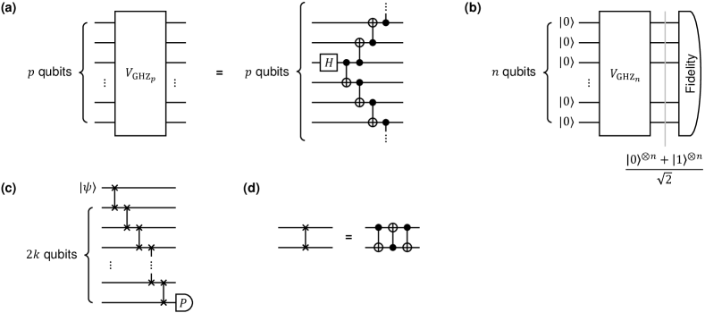
(a)

(b)

(c)

(d)

Figure S1: Additional circuit diagrams. (a) Structure of the $V_{\textsc{ghz}_{p}}$ block acting on $p$ qubits, which unitarily prepares a $p$-qubit GHZ state on an $\smash{\ket{0}^{\otimes p}}$ input. A Hadamard gate is applied on a qubit, and a fan-out of CX gates spanning all $p$ qubits follow. Thus $p-1$ CX gates are used, with depth $\lceil p/2\rceil$. (b) Unitary GHZ state preparation circuit as used in experiments (Sec. IV.2 of the main text) for comparison. (c) Unitary circuit that transports an input qubit state $\ket{\psi}$ a distance of $2k$ qubits, as used in staged quantum state teleportation experiments (Sec. IV.3 of the main text) for comparison. $P\in\{X,Y,Z\}$ denotes a Pauli-basis terminal measurement. (d) Standard decomposition of a SWAP gate into $3$ CX gates, which is optimal.

Device	Qubits	2Q Gate	1Q Gate Error ($\times 10^{-4}$)			2Q Gate Error ($\times 10^{-3}$)			Readout Error ($\times 10^{-2}$)
			P10	P90	Med.	P10	P90	Med.	P10	P90	Med.
ibm_osaka	127	ECR	1.23	12.5	2.41	4.03	19.3	7.15	0.65	8.94	1.99
ibm_kyoto	127	ECR	1.46	10.5	2.68	4.56	19.4	8.01	0.61	8.15	1.51
ibm_algiers	27	CX	1.83	8.23	2.84	5.88	15.3	8.90	0.59	3.59	1.01
ibmq_kolkata	27	CX	1.90	4.75	2.55	4.96	17.2	8.62	0.56	14.5	1.23
ibmq_mumbai	27	CX	1.58	3.75	2.08	5.66	11.5	7.52	1.24	5.87	1.70

Device	1Q Gate Time ($\mathrm{ns}$)	Readout Time ($\mathrm{ns}$)	2Q Gate Times ($\mathrm{ns}$)			$T_{1}$ ($\mathrm{\SIUnitSymbolMicro s}$)			$T_{2}$ ($\mathrm{\SIUnitSymbolMicro s}$)
			P10	P90	Med.	P10	P90	Med.	P10	P90	Med.
ibm_osaka	60	1400	660	660	660	127	396	275	19.8	322	151
ibm_kyoto	60	1400	660	660	660	124	320	223	28.2	237	115
ibm_algiers	35.6	910	263	622	370	93.1	184	136	44.3	252	144
ibmq_kolkata	35.6	640	391	556	462	58.5	139	96.4	22.8	119	63.8
ibmq_mumbai	35.6	3513	277	640	405	54.6	130	108	58.4	251	149

Table S2: Performance characteristics of quantum devices used in experiments. For quantities that vary between qubits on the same device, we provide $10^{\text{th}}$ and $90^{\text{th}}$ percentile and median values evaluated over all qubits on the device. Characteristics summarized here are based on routine (${\sim}$daily) calibration data of the machines, pulled over a duration of two weeks in the middle of experiments.

Appendix D Additional Experiment Results and Simulations

D.1 Mid-circuit dynamic qubit reset

D.1.1 Additional experiment results

As referenced in Sec. IV.1 of the main text, in Figure S2 we present additional experiment results acquired on two other superconducting quantum devices. The results are qualitatively similar to that shown in Figures 4b and 4c. In Figure S3 we include repetition-based readout error mitigation protocols Rep-ALL and Rep-MAJ at $r=3$, which are not at all competitive with PROM or even without readout error mitigation for mid-circuit measurements and feedforward.

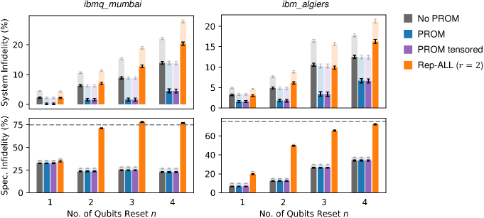
Figure S2: Additional dynamic qubit reset experiment results. Infidelities of system qubits after dynamic resets against the ideal $\smash{\ket{0}^{\otimes n}}$ post-reset state, and infidelities of spectator qubits against $\smash{\ket{0}^{\otimes 2}}$ after witnessing reset events conditioned on system qubits being correctly reset, comparing PROM, PROM assuming tensored readout channels, Rep-ALL at $r=2$, and without readout error mitigation for mid-circuit measurements and feedforward. Dashed line demarcates $75\%$ infidelity expected for a maximally mixed spectator state. In all plots, solid bars are with terminal readout error mitigation; translucent bars without. Experiment performed on superconducting quantum device ibmq_mumbai and ibm_algiers as labeled, complementing results on ibmq_kolkata as presented in Figures 4b and 4c of the main text. Error bars are standard deviations across $1000$ trials per qubit chain, each with $10000$ shots; data averaged over ${\sim}8$ randomly chosen qubit chains.

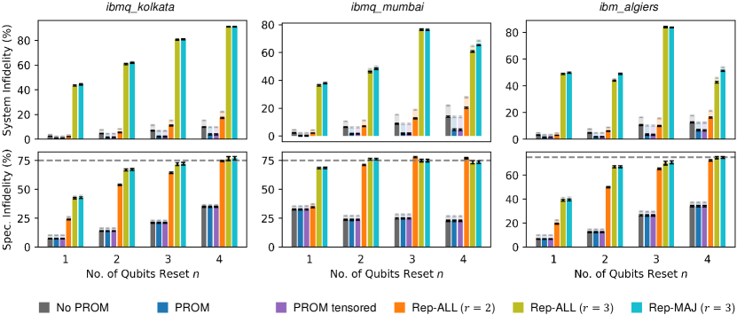
Figure S3: Additional dynamic qubit reset experiment results. Zoomed-out version of Figures 4b and 4c of the main text and Figure S2 that includes repetition-based readout error mitigation methods Rep-ALL and Rep-MAJ at $r=3$.

D.2 Shallow-depth GHZ state preparation

D.2.1 Additional experiment results

As referenced in Sec. IV.2 of the main text, in Figure S4a we present additional experiment results acquired on a second superconducting quantum device for GHZ system sizes $n=4,6$. The results are qualitatively similar to that shown in Figure 5b. In Figure S4b we include repetition-based readout error mitigation protocols Rep-ALL and Rep-MAJ at $r=3$, which are not at all competitive with PROM or even without readout error mitigation for mid-circuit measurements and feedforward.

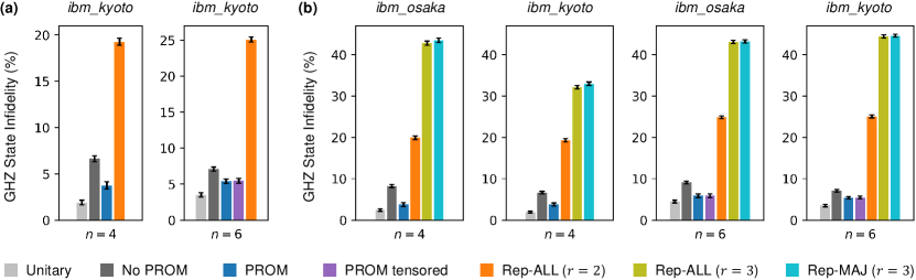
(a)

(b)

Figure S4: Additional GHZ state preparation experiment results. (a) Infidelities of the prepared state against the ideal $n$-qubit GHZ state, comparing PROM, PROM assuming tensored readout channels, Rep-ALL at $r=2$, and without readout error mitigation for mid-circuit measurements and feedforward. Also shown are infidelities on a unitary circuit without feedforward ($\smash{V_{\textsc{ghz}_{n}}}$) for comparison. Data acquired on the ibm_kyoto superconducting quantum device, complementing results on ibm_osaka as presented in Figure 5b of the main text. (b) Zoomed-out version of Figure 5b of the main text and (a) that includes repetition-based readout error mitigation methods Rep-ALL and Rep-MAJ at $r=3$. Readout error mitigation for terminal measurements was applied for all data. The $n=4,6$ experiments employ $(b,p)=(2,1)$, $(3,1)$ circuit structures respectively. Error bars are standard deviations across $100$ trials each with $10000$ shots.

D.3 Staged quantum state teleportation

D.3.1 Additional experiment results

As referenced in Sec. IV.3 of the main text, in Figure S5 we present additional experiment results acquired on a second superconducting quantum device. The results are qualitatively similar to that shown in Figure 6b. In Figure S6 we include repetition-based readout error mitigation protocol Rep-ALL at $r=2$, which is not at all competitive with PROM or even without readout error mitigation for mid-circuit measurements and feedforward.

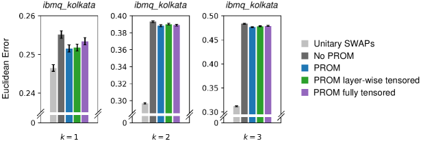
Figure S5: Additional quantum state teleportation experiment results. Euclidean errors $\smash{\Delta=(\delta X^{2}+\delta Y^{2}+\delta Z^{2})^{1/2}}$ after $k\in\{1,2,3\}$ teleportations, comparing PROM, PROM assuming layer-wise and fully tensored readout channels, and without readout error mitigation for mid-circuit measurements and feedforward. Also shown are errors on a unitary circuit with SWAP gates that transport the input state $\ket{\psi}$ across the same qubits. Readout error mitigation for terminal measurements was applied for all data. Experiments performed on the superconducting quantum device ibmq_kolkata, complementing results on ibm_osaka as presented in Figure 6b of the main text. Error bars are standard deviations across $100$ trials each with $1000000$ shots.

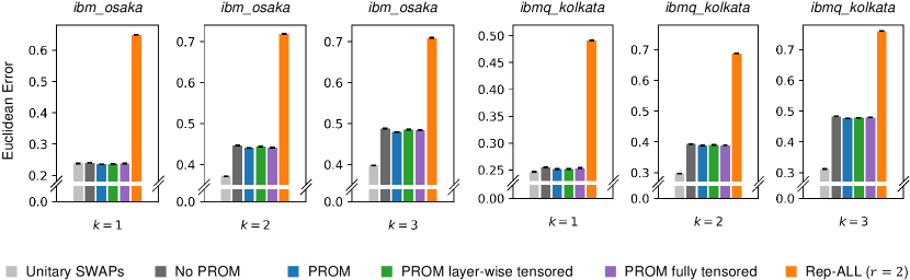
Figure S6: Additional quantum state teleportation experiment results. Zoomed-out version of Figure 6b of the main text and Figure S5 that includes repetition-based readout error mitigation method Rep-ALL at $r=2$.

References

- Ryan et al. [2017] C. A. Ryan, B. R. Johnson, D. Ristè, B. Donovan, and T. A. Ohki, Hardware for dynamic quantum computing, Rev. Sci. Instrum. 88, 104703 (2017).
- Pino et al. [2021] J. M. Pino, J. M. Dreiling, C. Figgatt, J. P. Gaebler, S. A. Moses, M. Allman, C. Baldwin, M. Foss-Feig, D. Hayes, K. Mayer, et al., Demonstration of the trapped-ion quantum CCD computer architecture, Nature 592, 209 (2021).
- Moses et al. [2023] S. A. Moses, C. H. Baldwin, M. S. Allman, R. Ancona, L. Ascarrunz, C. Barnes, J. Bartolotta, B. Bjork, P. Blanchard, M. Bohn, et al., A race-track trapped-ion quantum processor, Phys. Rev. X 13, 041052 (2023).
- Graham et al. [2023] T. M. Graham, L. Phuttitarn, R. Chinnarasu, Y. Song, C. Poole, K. Jooya, J. Scott, A. Scott, P. Eichler, and M. Saffman, Midcircuit measurements on a single-species neutral alkali atom quantum processor, Phys. Rev. X 13, 041051 (2023).
- Córcoles et al. [2021] A. D. Córcoles, M. Takita, K. Inoue, S. Lekuch, Z. K. Minev, J. M. Chow, and J. M. Gambetta, Exploiting dynamic quantum circuits in a quantum algorithm with superconducting qubits, Phys. Rev. Lett. 127, 100501 (2021).
- Gottesman [2010] D. Gottesman, An introduction to quantum error correction and fault-tolerant quantum computation, in Quantum information science and its contributions to mathematics, Proceedings of Symposia in Applied Mathematics, Vol. 68 (2010) pp. 13–58.
- Acharya et al. [2023] R. Acharya, I. Aleiner, R. Allen, T. I. Andersen, M. Ansmann, F. Arute, K. Arya, A. Asfaw, J. Atalaya, R. Babbush, et al., Suppressing quantum errors by scaling a surface code logical qubit, Nature 614, 676 (2023).
- Sivak et al. [2023] V. Sivak, A. Eickbusch, B. Royer, S. Singh, I. Tsioutsios, S. Ganjam, A. Miano, B. Brock, A. Ding, L. Frunzio, et al., Real-time quantum error correction beyond break-even, Nature 616, 50 (2023).
- Sundaresan et al. [2023] N. Sundaresan, T. J. Yoder, Y. Kim, M. Li, E. H. Chen, G. Harper, T. Thorbeck, A. W. Cross, A. D. Córcoles, and M. Takita, Demonstrating multi-round subsystem quantum error correction using matching and maximum likelihood decoders, Nat. Commun. 14, 2852 (2023).
- Rost et al. [2021] B. Rost, L. D. Re, N. Earnest, A. F. Kemper, B. Jones, and J. K. Freericks, Demonstrating robust simulation of driven-dissipative problems on near-term quantum computers (2021), arXiv:2108.01183 [quant-ph] .
- Han et al. [2021] J. Han, W. Cai, L. Hu, X. Mu, Y. Ma, Y. Xu, W. Wang, H. Wang, Y. P. Song, C.-L. Zou, and L. Sun, Experimental simulation of open quantum system dynamics via Trotterization, Phys. Rev. Lett. 127, 020504 (2021).
- Del Re et al. [2024] L. Del Re, B. Rost, M. Foss-Feig, A. F. Kemper, and J. K. Freericks, Robust measurements of -point correlation functions of driven-dissipative quantum systems on a digital quantum computer, Phys. Rev. Lett. 132, 100601 (2024).
- DeCross et al. [2023] M. DeCross, E. Chertkov, M. Kohagen, and M. Foss-Feig, Qubit-reuse compilation with mid-circuit measurement and reset, Phys. Rev. X 13, 041057 (2023).
- Bäumer et al. [2023] E. Bäumer, V. Tripathi, D. S. Wang, P. Rall, E. H. Chen, S. Majumder, A. Seif, and Z. K. Minev, Efficient long-range entanglement using dynamic circuits (2023), arXiv:2308.13065 [quant-ph] .
- Zhu et al. [2023] G.-Y. Zhu, N. Tantivasadakarn, A. Vishwanath, S. Trebst, and R. Verresen, Nishimori’s cat: Stable long-range entanglement from finite-depth unitaries and weak measurements, Phys. Rev. Lett. 131, 200201 (2023).
- Tantivasadakarn et al. [2023] N. Tantivasadakarn, R. Verresen, and A. Vishwanath, Shortest route to non-Abelian topological order on a quantum processor, Phys. Rev. Lett. 131, 060405 (2023).
- Foss-Feig et al. [2023] M. Foss-Feig, A. Tikku, T.-C. Lu, K. Mayer, M. Iqbal, T. M. Gatterman, J. A. Gerber, K. Gilmore, D. Gresh, A. Hankin, N. Hewitt, C. V. Horst, M. Matheny, T. Mengle, B. Neyenhuis, H. Dreyer, D. Hayes, T. H. Hsieh, and I. H. Kim, Experimental demonstration of the advantage of adaptive quantum circuits (2023), arXiv:2302.03029 [quant-ph] .
- Smith et al. [2023] K. C. Smith, E. Crane, N. Wiebe, and S. Girvin, Deterministic constant-depth preparation of the AKLT state on a quantum processor using fusion measurements, PRX Quantum 4, 020315 (2023).
- Iqbal et al. [2024] M. Iqbal, N. Tantivasadakarn, R. Verresen, S. L. Campbell, J. M. Dreiling, C. Figgatt, J. P. Gaebler, J. Johansen, M. Mills, S. A. Moses, et al., Non-Abelian topological order and anyons on a trapped-ion processor, Nature 626, 505 (2024).
- Bäumer et al. [2024] E. Bäumer, V. Tripathi, A. Seif, D. Lidar, and D. S. Wang, Quantum Fourier transform using dynamic circuits (2024), arXiv:2403.09514 [quant-ph] .
- Piveteau and Sutter [2024] C. Piveteau and D. Sutter, Circuit knitting with classical communication, IEEE Trans. Inf. Theory 70, 2734 (2024).
- Vazquez et al. [2024] A. C. Vazquez, C. Tornow, D. Riste, S. Woerner, M. Takita, and D. J. Egger, Scaling quantum computing with dynamic circuits (2024), arXiv:2402.17833 [quant-ph] .
- Pirandola et al. [2015] S. Pirandola, J. Eisert, C. Weedbrook, A. Furusawa, and S. L. Braunstein, Advances in quantum teleportation, Nat. Photonics 9, 641 (2015).
- Wan et al. [2019] Y. Wan, D. Kienzler, S. D. Erickson, K. H. Mayer, T. R. Tan, J. J. Wu, H. M. Vasconcelos, S. Glancy, E. Knill, D. J. Wineland, et al., Quantum gate teleportation between separated qubits in a trapped-ion processor, Science 364, 875 (2019).
- Hu et al. [2023] X.-M. Hu, Y. Guo, B.-H. Liu, C.-F. Li, and G.-C. Guo, Progress in quantum teleportation, Nat. Rev. Phys. 5, 339 (2023).
- Zwierz et al. [2010] M. Zwierz, C. A. Pérez-Delgado, and P. Kok, General optimality of the Heisenberg limit for quantum metrology, Phys. Rev. Lett. 105, 180402 (2010).
- Becerra et al. [2013] F. Becerra, J. Fan, G. Baumgartner, J. Goldhar, J. Kosloski, and A. Migdall, Experimental demonstration of a receiver beating the standard quantum limit for multiple nonorthogonal state discrimination, Nat. Photonics 7, 147 (2013).
- Demkowicz-Dobrzański et al. [2017] R. Demkowicz-Dobrzański, J. Czajkowski, and P. Sekatski, Adaptive quantum metrology under general Markovian noise, Phys. Rev. X 7, 041009 (2017).
- Knill [2005] E. Knill, Quantum computing with realistically noisy devices, Nature 434, 39 (2005).
- Bartolucci et al. [2023] S. Bartolucci, P. Birchall, H. Bombin, H. Cable, C. Dawson, M. Gimeno-Segovia, E. Johnston, K. Kieling, N. Nickerson, M. Pant, et al., Fusion-based quantum computation, Nat. Commun. 14, 912 (2023).
- Gupta et al. [2024] R. S. Gupta, N. Sundaresan, T. Alexander, C. J. Wood, S. T. Merkel, M. B. Healy, M. Hillenbrand, T. Jochym-O’Connor, J. R. Wootton, T. J. Yoder, et al., Encoding a magic state with beyond break-even fidelity, Nature 625, 259 (2024).
- Cong et al. [2019] I. Cong, S. Choi, and M. D. Lukin, Quantum convolutional neural networks, Nat. Phys. 15, 1273 (2019).
- Cai et al. [2023] Z. Cai, R. Babbush, S. C. Benjamin, S. Endo, W. J. Huggins, Y. Li, J. R. McClean, and T. E. O’Brien, Quantum error mitigation, Rev. Mod. Phys. 95, 045005 (2023).
- Lin et al. [2021] J. Lin, J. J. Wallman, I. Hincks, and R. Laflamme, Independent state and measurement characterization for quantum computers, Phys. Rev. Res. 3, 033285 (2021).
- Kandala et al. [2017] A. Kandala, A. Mezzacapo, K. Temme, M. Takita, M. Brink, J. M. Chow, and J. M. Gambetta, Hardware-efficient variational quantum eigensolver for small molecules and quantum magnets, Nature 549, 242 (2017).
- Kandala et al. [2019] A. Kandala, K. Temme, A. D. Córcoles, A. Mezzacapo, J. M. Chow, and J. M. Gambetta, Error mitigation extends the computational reach of a noisy quantum processor, Nature 567, 491 (2019).
- Jurcevic et al. [2021] P. Jurcevic, A. Javadi-Abhari, L. S. Bishop, I. Lauer, D. F. Bogorin, M. Brink, L. Capelluto, O. Günlük, T. Itoko, N. Kanazawa, et al., Demonstration of quantum volume 64 on a superconducting quantum computing system, Quantum Sci. Technol. 6, 025020 (2021).
- Van Den Berg et al. [2023] E. Van Den Berg, Z. K. Minev, A. Kandala, and K. Temme, Probabilistic error cancellation with sparse Pauli–Lindblad models on noisy quantum processors, Nat. Phys. 19, 1116 (2023).
- Gupta et al. [2023] R. S. Gupta, E. van den Berg, M. Takita, D. Riste, K. Temme, and A. Kandala, Probabilistic error cancellation for dynamic quantum circuits (2023), arXiv:2310.07825 [quant-ph] .
- Li and Benjamin [2017] Y. Li and S. C. Benjamin, Efficient variational quantum simulator incorporating active error minimization, Phys. Rev. X 7, 021050 (2017).
- Temme et al. [2017] K. Temme, S. Bravyi, and J. M. Gambetta, Error mitigation for short-depth quantum circuits, Phys. Rev. Lett. 119, 180509 (2017).
- Giurgica-Tiron et al. [2020] T. Giurgica-Tiron, Y. Hindy, R. LaRose, A. Mari, and W. J. Zeng, Digital zero noise extrapolation for quantum error mitigation, in 2020 IEEE International Conference on Quantum Computing and Engineering (QCE) (IEEE, 2020) pp. 306–316.
- Czarnik et al. [2021] P. Czarnik, A. Arrasmith, P. J. Coles, and L. Cincio, Error mitigation with Clifford quantum-circuit data, Quantum 5, 592 (2021).
- Liao et al. [2023] H. Liao, D. S. Wang, I. Sitdikov, C. Salcedo, A. Seif, and Z. K. Minev, Machine learning for practical quantum error mitigation (2023), arXiv:2309.17368 [quant-ph] .
- Wallman and Emerson [2016] J. J. Wallman and J. Emerson, Noise tailoring for scalable quantum computation via randomized compiling, Phys. Rev. A 94, 052325 (2016).
- Hashim et al. [2021] A. Hashim, R. K. Naik, A. Morvan, J.-L. Ville, B. Mitchell, J. M. Kreikebaum, M. Davis, E. Smith, C. Iancu, K. P. O’Brien, I. Hincks, J. J. Wallman, J. Emerson, and I. Siddiqi, Randomized compiling for scalable quantum computing on a noisy superconducting quantum processor, Phys. Rev. X 11, 041039 (2021).
- Sun et al. [2024] S.-N. Sun, B. Marinelli, J. M. Koh, Y. Kim, L. B. Nguyen, L. Chen, J. M. Kreikebaum, D. I. Santiago, I. Siddiqi, and A. J. Minnich, Quantum computation of frequency-domain molecular response properties using a three-qubit itoffoli gate, npj Quantum Inf. 10, 55 (2024).
- Chow et al. [2010] J. M. Chow, L. DiCarlo, J. M. Gambetta, A. Nunnenkamp, L. S. Bishop, L. Frunzio, M. H. Devoret, S. M. Girvin, and R. J. Schoelkopf, Detecting highly entangled states with a joint qubit readout, Phys. Rev. A 81, 062325 (2010).
- Nation et al. [2021] P. D. Nation, H. Kang, N. Sundaresan, and J. M. Gambetta, Scalable mitigation of measurement errors on quantum computers, PRX Quantum 2, 040326 (2021).
- Bravyi et al. [2021] S. Bravyi, S. Sheldon, A. Kandala, D. C. Mckay, and J. M. Gambetta, Mitigating measurement errors in multiqubit experiments, Phys. Rev. A 103, 042605 (2021).
- Barron and Wood [2020] G. S. Barron and C. J. Wood, Measurement error mitigation for variational quantum algorithms (2020), arXiv:2010.08520 [quant-ph] .
- Smith et al. [2021] A. W. Smith, K. E. Khosla, C. N. Self, and M. Kim, Qubit readout error mitigation with bit-flip averaging, Sci. Adv. 7, eabi8009 (2021).
- Hicks et al. [2021] R. Hicks, C. W. Bauer, and B. Nachman, Readout rebalancing for near-term quantum computers, Phys. Rev. A 103, 022407 (2021).
- Emerson et al. [2007] J. Emerson, M. Silva, O. Moussa, C. Ryan, M. Laforest, J. Baugh, D. G. Cory, and R. Laflamme, Symmetrized characterization of noisy quantum processes, Science 317, 1893 (2007).
- Bennett et al. [1996] C. H. Bennett, G. Brassard, S. Popescu, B. Schumacher, J. A. Smolin, and W. K. Wootters, Purification of noisy entanglement and faithful teleportation via noisy channels, Phys. Rev. Lett. 76, 722 (1996).
- Knill [2004] E. Knill, Fault-tolerant postselected quantum computation: Threshold analysis (2004), arXiv:quant-ph/0404104 [quant-ph] .
- Kern et al. [2005] O. Kern, G. Alber, and D. L. Shepelyansky, Quantum error correction of coherent errors by randomization, Eur. Phys. J. D 32, 153 (2005).
- Geller and Zhou [2013] M. R. Geller and Z. Zhou, Efficient error models for fault-tolerant architectures and the Pauli twirling approximation, Phys. Rev. A 88, 012314 (2013).
- Chen et al. [2021] S. Chen, W. Yu, P. Zeng, and S. T. Flammia, Robust shadow estimation, PRX Quantum 2, 030348 (2021).
- Ahmed and Rao [1975] N. Ahmed and K. R. Rao, Walsh-Hadamard transform, in Orthogonal Transforms for Digital Signal Processing (Springer Berlin Heidelberg, Berlin, Heidelberg, 1975) pp. 99–152.
- Beer [1981] T. Beer, Walsh transforms, Am. J. Phys. 49, 466 (1981).
- Marsaglia et al. [2004] G. Marsaglia, W. W. Tsang, and J. Wang, Fast generation of discrete random variables, J. Stat. Softw. 11, 1 (2004).
- Vose [1991] M. D. Vose, A linear algorithm for generating random numbers with a given distribution, IEEE Trans. Softw. Eng. 17, 972 (1991).
- Walker [1977] A. J. Walker, An efficient method for generating discrete random variables with general distributions, ACM Trans. Math. Softw. 3, 253 (1977).
- Suter and Álvarez [2016] D. Suter and G. A. Álvarez, Colloquium: Protecting quantum information against environmental noise, Rev. Mod. Phys. 88, 041001 (2016).
- Clerk et al. [2010] A. A. Clerk, M. H. Devoret, S. M. Girvin, F. Marquardt, and R. J. Schoelkopf, Introduction to quantum noise, measurement, and amplification, Rev. Mod. Phys. 82, 1155 (2010).
- Nielsen and Chuang [2010] M. A. Nielsen and I. L. Chuang, Quantum computation and quantum information (Cambridge university press, 2010).
- DiVincenzo [2000] D. P. DiVincenzo, The physical implementation of quantum computation, Fortschr. Phys. 48, 771 (2000).
- Ristè et al. [2012] D. Ristè, J. G. van Leeuwen, H.-S. Ku, K. W. Lehnert, and L. DiCarlo, Initialization by measurement of a superconducting quantum bit circuit, Phys. Rev. Lett. 109, 050507 (2012).
- Bartolomeo et al. [2023] G. D. Bartolomeo, M. Vischi, T. Feri, A. Bassi, and S. Donadi, Efficient quantum algorithm to simulate open systems through the quantum noise formalism (2023), arXiv:2311.10009 [quant-ph] .
- Hua et al. [2023] F. Hua, Y. Jin, Y. Chen, S. Vittal, K. Krsulich, L. S. Bishop, J. Lapeyre, A. Javadi-Abhari, and E. Z. Zhang, Exploiting qubit reuse through mid-circuit measurement and reset (2023), arXiv:2211.01925 [quant-ph] .
- Yirka and Subaşı [2021] J. Yirka and Y. Subaşı, Qubit-efficient entanglement spectroscopy using qubit resets, Quantum 5, 535 (2021).
- Heußen et al. [2024] S. Heußen, D. F. Locher, and M. Müller, Measurement-free fault-tolerant quantum error correction in near-term devices, PRX Quantum 5, 010333 (2024).
- Perlin et al. [2023] M. A. Perlin, V. N. Premakumar, J. Wang, M. Saffman, and R. Joynt, Fault-tolerant measurement-free quantum error correction with multiqubit gates, Phys. Rev. A 108, 062426 (2023).
- Childs and Wiebe [2012] A. M. Childs and N. Wiebe, Hamiltonian simulation using linear combinations of unitary operations, Quantum Inf. Comput. 12, 0901 (2012).
- Berry et al. [2015] D. W. Berry, A. M. Childs, R. Cleve, R. Kothari, and R. D. Somma, Simulating Hamiltonian dynamics with a truncated Taylor series, Phys. Rev. Lett. 114, 090502 (2015).
- Gilyén et al. [2019] A. Gilyén, Y. Su, G. H. Low, and N. Wiebe, Quantum singular value transformation and beyond: exponential improvements for quantum matrix arithmetics, in Proceedings of the 51st Annual ACM SIGACT Symposium on Theory of Computing (2019) pp. 193–204.
- Dong et al. [2021] Q. Dong, M. T. Quintino, A. Soeda, and M. Murao, Success-or-draw: A strategy allowing repeat-until-success in quantum computation, Phys. Rev. Lett. 126, 150504 (2021).
- Greenberger et al. [1990] D. M. Greenberger, M. A. Horne, A. Shimony, and A. Zeilinger, Bell’s theorem without inequalities, Am. J. Phys. 58, 1131 (1990).
- Leibfried et al. [2004] D. Leibfried, M. D. Barrett, T. Schaetz, J. Britton, J. Chiaverini, W. M. Itano, J. D. Jost, C. Langer, and D. J. Wineland, Toward Heisenberg-limited spectroscopy with multiparticle entangled states, Science 304, 1476 (2004).
- Liao et al. [2014] C.-H. Liao, C.-W. Yang, and T. Hwang, Dynamic quantum secret sharing protocol based on GHZ state, Quantum Inf. Process. 13, 1907 (2014).
- Hahn et al. [2020] F. Hahn, J. de Jong, and A. Pappa, Anonymous quantum conference key agreement, PRX Quantum 1, 020325 (2020).
- Watts et al. [2019] A. B. Watts, R. Kothari, L. Schaeffer, and A. Tal, Exponential separation between shallow quantum circuits and unbounded fan-in shallow classical circuits, in Proceedings of the 51st Annual ACM SIGACT Symposium on Theory of Computing (2019) pp. 515–526.
- Quek et al. [2024a] Y. Quek, E. Kaur, and M. M. Wilde, Multivariate trace estimation in constant quantum depth, Quantum 8, 1220 (2024a).
- Bennett et al. [1993] C. H. Bennett, G. Brassard, C. Crépeau, R. Jozsa, A. Peres, and W. K. Wootters, Teleporting an unknown quantum state via dual classical and einstein-podolsky-rosen channels, Phys. Rev. Lett. 70, 1895 (1993).
- Bouwmeester et al. [1997] D. Bouwmeester, J.-W. Pan, K. Mattle, M. Eibl, H. Weinfurter, and A. Zeilinger, Experimental quantum teleportation, Nature 390, 575 (1997).
- Ren et al. [2017] J.-G. Ren, P. Xu, H.-L. Yong, L. Zhang, S.-K. Liao, J. Yin, W.-Y. Liu, W.-Q. Cai, M. Yang, L. Li, et al., Ground-to-satellite quantum teleportation, Nature 549, 70 (2017).
- Martiel and de Brugière [2022] S. Martiel and T. G. de Brugière, Architecture aware compilation of quantum circuits via lazy synthesis, Quantum 6, 729 (2022).
- Wagner et al. [2023] F. Wagner, A. Bärmann, F. Liers, and M. Weissenbäck, Improving quantum computation by optimized qubit routing, J. Optim. Theory Appl. 197, 1161 (2023).
- Takagi et al. [2023] R. Takagi, H. Tajima, and M. Gu, Universal sampling lower bounds for quantum error mitigation, Phys. Rev. Lett. 131, 210602 (2023).
- Takagi et al. [2022] R. Takagi, S. Endo, S. Minagawa, and M. Gu, Fundamental limits of quantum error mitigation, npj Quantum Inf. 8, 114 (2022).
- Quek et al. [2024b] Y. Quek, D. S. França, S. Khatri, J. J. Meyer, and J. Eisert, Exponentially tighter bounds on limitations of quantum error mitigation (2024b), arXiv:2210.11505 [quant-ph] .
- Yuan et al. [2024] X. Yuan, B. Regula, R. Takagi, and M. Gu, Virtual quantum resource distillation, Phys. Rev. Lett. 132, 050203 (2024).
- Takagi et al. [2024] R. Takagi, X. Yuan, B. Regula, and M. Gu, Virtual quantum resource distillation: General framework and applications, Phys. Rev. A 109, 022403 (2024).
- Regula and Takagi [2021] B. Regula and R. Takagi, Fundamental limitations on distillation of quantum channel resources, Nat. Commun. 12, 4411 (2021).
- Liu and Yuan [2020] Y. Liu and X. Yuan, Operational resource theory of quantum channels, Phys. Rev. Res. 2, 012035 (2020).
- Hashim et al. [2024] A. Hashim, A. Carignan-Dugas, L. Chen, C. Juenger, N. Fruitwala, Y. Xu, G. Huang, J. J. Wallman, and I. Siddiqi, Quasi-probabilistic readout correction of mid-circuit measurements for adaptive feedback via measurement randomized compiling (2024), arXiv:2312.14139 [quant-ph] .
- Ivashkov et al. [2023] P. Ivashkov, G. Uchehara, L. Jiang, D. S. Wang, and A. Seif, High-fidelity, multi-qubit generalized measurements with dynamic circuits (2023), arXiv:2312.14087 [quant-ph] .
- Fino and Algazi [1976] Fino and Algazi, Unified matrix treatment of the fast walsh-hadamard transform, IEEE Trans. Comput. 100, 1142 (1976).
- Walker [1974] A. J. Walker, New fast method for generating discrete random numbers with arbitrary frequency distributions, Electron. Lett. 8, 127 (1974).
- Yuan et al. [2021] X. Yuan, Y. Liu, Q. Zhao, B. Regula, J. Thompson, and M. Gu, Universal and operational benchmarking of quantum memories, npj Quantum Inf. 7, 108 (2021).
- Deif [1986] A. Deif, Perturbation of linear equations, in Sensitivity Analysis in Linear Systems (Springer Berlin Heidelberg, Berlin, Heidelberg, 1986) pp. 1–43.
- Rohn [1989] J. Rohn, New condition numbers for matrices and linear systems, Computing 41, 167 (1989).
- McKay et al. [2017] D. C. McKay, C. J. Wood, S. Sheldon, J. M. Chow, and J. M. Gambetta, Efficient gates for quantum computing, Phys. Rev. A 96, 022330 (2017).
- Sundaresan et al. [2020] N. Sundaresan, I. Lauer, E. Pritchett, E. Magesan, P. Jurcevic, and J. M. Gambetta, Reducing unitary and spectator errors in cross resonance with optimized rotary echoes, PRX Quantum 1, 020318 (2020).
- Smolin et al. [2012] J. A. Smolin, J. M. Gambetta, and G. Smith, Efficient method for computing the maximum-likelihood quantum state from measurements with additive gaussian noise, Phys. Rev. Lett. 108, 070502 (2012).
- Geller [2020] M. R. Geller, Rigorous measurement error correction, Quantum Sci. Technol. 5, 03LT01 (2020).
- Maciejewski et al. [2020] F. B. Maciejewski, Z. Zimborás, and M. Oszmaniec, Mitigation of readout noise in near-term quantum devices by classical post-processing based on detector tomography, Quantum 4, 257 (2020).
- Nachman et al. [2020] B. Nachman, M. Urbanek, W. A. de Jong, and C. W. Bauer, Unfolding quantum computer readout noise, npj Quantum Inf. 6, 84 (2020).
- Koh et al. [2022a] J. M. Koh, T. Tai, and C. H. Lee, Simulation of interaction-induced chiral topological dynamics on a digital quantum computer, Phys. Rev. Lett. 129, 140502 (2022a).
- Koh et al. [2022b] J. M. Koh, T. Tai, Y. H. Phee, W. E. Ng, and C. H. Lee, Stabilizing multiple topological fermions on a quantum computer, npj Quantum Inf. 8, 16 (2022b).
- Koh et al. [2023a] J. M. Koh, S.-N. Sun, M. Motta, and A. J. Minnich, Measurement-induced entanglement phase transition on a superconducting quantum processor with mid-circuit readout, Nat. Phys. 19, 1314 (2023a).
- Koh et al. [2023b] J. M. Koh, T. Tai, and C. H. Lee, Observation of higher-order topological states on a quantum computer (2023b), arXiv:2303.02179 [cond-mat.str-el] .
- Viola et al. [1999] L. Viola, E. Knill, and S. Lloyd, Dynamical decoupling of open quantum systems, Phys. Rev. Lett. 82, 2417 (1999).
- Kim et al. [2023a] Y. Kim, C. J. Wood, T. J. Yoder, S. T. Merkel, J. M. Gambetta, K. Temme, and A. Kandala, Scalable error mitigation for noisy quantum circuits produces competitive expectation values, Nat. Phys. 19, 752 (2023a).
- Pokharel et al. [2018] B. Pokharel, N. Anand, B. Fortman, and D. A. Lidar, Demonstration of fidelity improvement using dynamical decoupling with superconducting qubits, Phys. Rev. Lett. 121, 220502 (2018).
- Khodjasteh and Lidar [2005] K. Khodjasteh and D. A. Lidar, Fault-tolerant quantum dynamical decoupling, Phys. Rev. Lett. 95, 180501 (2005).
- Uhrig [2007] G. S. Uhrig, Keeping a quantum bit alive by optimized -pulse sequences, Phys. Rev. Lett. 98, 100504 (2007).
- Ezzell et al. [2023] N. Ezzell, B. Pokharel, L. Tewala, G. Quiroz, and D. A. Lidar, Dynamical decoupling for superconducting qubits: A performance survey, Phys. Rev. Appl. 20, 064027 (2023).
- Pokharel and Lidar [2024] B. Pokharel and D. A. Lidar, Better-than-classical grover search via quantum error detection and suppression, npj Quantum Inf. 10, 23 (2024).
- Pokharel and Lidar [2023] B. Pokharel and D. A. Lidar, Demonstration of algorithmic quantum speedup, Phys. Rev. Lett. 130, 210602 (2023).
- Kim et al. [2023b] Y. Kim, A. Eddins, S. Anand, K. X. Wei, E. Van Den Berg, S. Rosenblatt, H. Nayfeh, Y. Wu, M. Zaletel, K. Temme, et al., Evidence for the utility of quantum computing before fault tolerance, Nature 618, 500 (2023b).
- Tong et al. [2024] C. Tong, H. Zhang, and B. Pokharel, Empirical learning of dynamical decoupling on quantum processors (2024), arXiv:2403.02294 [quant-ph] .
- Buhrman et al. [2001] H. Buhrman, R. Cleve, J. Watrous, and R. de Wolf, Quantum fingerprinting, Phys. Rev. Lett. 87, 167902 (2001).
- Barenco et al. [1997] A. Barenco, A. Berthiaume, D. Deutsch, A. Ekert, R. Jozsa, and C. Macchiavello, Stabilization of quantum computations by symmetrization, SIAM J. Comput. 26, 1541 (1997).
- Flammia and Liu [2011] S. T. Flammia and Y.-K. Liu, Direct fidelity estimation from few Pauli measurements, Phys. Rev. Lett. 106, 230501 (2011).
- da Silva et al. [2011] M. P. da Silva, O. Landon-Cardinal, and D. Poulin, Practical characterization of quantum devices without tomography, Phys. Rev. Lett. 107, 210404 (2011).
- Cao et al. [2023] S. Cao, B. Wu, F. Chen, M. Gong, Y. Wu, Y. Ye, C. Zha, H. Qian, C. Ying, S. Guo, et al., Generation of genuine entanglement up to 51 superconducting qubits, Nature 619, 738 (2023).
- Gokhale et al. [2019] P. Gokhale, O. Angiuli, Y. Ding, K. Gui, T. Tomesh, M. Suchara, M. Martonosi, and F. T. Chong, Minimizing state preparations in variational quantum eigensolver by partitioning into commuting families (2019), arXiv:1907.13623 [quant-ph] .
- Sackett et al. [2000] C. A. Sackett, D. Kielpinski, B. E. King, C. Langer, V. Meyer, C. J. Myatt, M. Rowe, Q. Turchette, W. M. Itano, D. J. Wineland, et al., Experimental entanglement of four particles, Nature 404, 256 (2000).
- Leibfried et al. [2005] D. Leibfried, E. Knill, S. Seidelin, J. Britton, R. B. Blakestad, J. Chiaverini, D. B. Hume, W. M. Itano, J. D. Jost, C. Langer, et al., Creation of a six-atom ‘Schrödinger cat’ state, Nature 438, 639 (2005).
- Monz et al. [2011] T. Monz, P. Schindler, J. T. Barreiro, M. Chwalla, D. Nigg, W. A. Coish, M. Harlander, W. Hänsel, M. Hennrich, and R. Blatt, 14-qubit entanglement: Creation and coherence, Phys. Rev. Lett. 106, 130506 (2011).
- Omran et al. [2019] A. Omran, H. Levine, A. Keesling, G. Semeghini, T. T. Wang, S. Ebadi, H. Bernien, A. S. Zibrov, H. Pichler, S. Choi, et al., Generation and manipulation of Schrödinger cat states in Rydberg atom arrays, Science 365, 570 (2019).
- Pogorelov et al. [2021] I. Pogorelov, T. Feldker, C. D. Marciniak, L. Postler, G. Jacob, O. Krieglsteiner, V. Podlesnic, M. Meth, V. Negnevitsky, M. Stadler, B. Höfer, C. Wächter, K. Lakhmanskiy, R. Blatt, P. Schindler, and T. Monz, Compact ion-trap quantum computing demonstrator, PRX Quantum 2, 020343 (2021).
- Thomas et al. [2022] P. Thomas, L. Ruscio, O. Morin, and G. Rempe, Efficient generation of entangled multiphoton graph states from a single atom, Nature 608, 677 (2022).
- Mooney et al. [2021] G. J. Mooney, G. A. White, C. D. Hill, and L. C. Hollenberg, Generation and verification of 27-qubit Greenberger-Horne-Zeilinger states in a superconducting quantum computer, J. Phys. Commun. 5, 095004 (2021).
- Wei et al. [2020] K. X. Wei, I. Lauer, S. Srinivasan, N. Sundaresan, D. T. McClure, D. Toyli, D. C. McKay, J. M. Gambetta, and S. Sheldon, Verifying multipartite entangled Greenberger-Horne-Zeilinger states via multiple quantum coherences, Phys. Rev. A 101, 032343 (2020).