Probing fundamental physics with Extreme Mass Ratio Inspirals:
a full Bayesian inference for scalar charge

Abstract

Extreme Mass Ratio Inspirals (EMRIs) are key sources for the future space-based gravitational wave detector LISA, and are considered promising probes of fundamental physics. Here, we present the first complete Bayesian analysis of EMRI signals in theories with an additional massless scalar, which could arise in an extension of General Relativity or of the Standard Model of Particle Physics. We develop a waveform model accurate at adiabatic order for equatorial eccentric orbits around spinning black holes. Using full Bayesian inference, we forecast LISA’s ability to probe the presence of new fundamental fields with EMRI observations.

Introduction. In the last decade, gravitational wave (GW) astronomy has revolutionized our ability to observe the Universe, offering unique opportunities to test the nature of gravity and search for new fundamental fields in previously unexplored regimes [1, 2, 3]. Observations with gravitational-wave detectors allow us to probe the highly dynamic and strong-field regime of compact binary coalescences.

Ground-based interferometers have paved the way for searches for new physics beyond General Relativity (GR) or the Standard Model (SM) [4]. The constraining power of current facilities is limited to signal-to-noise ratio up to $30$ [5], comparable mass binaries, with the most asymmetric system detected so far having a mass ratio of $q\sim 1/10$ with GW190814 [6, 7, 8]. The next generation of ground-based detectors, such as the Einstein Telescope [9] and Cosmic Explorer [10], along with space-based missions like the Laser Interferometer Space Antenna (LISA) [11], TianQin [12], and Lunar Gravitational Wave Antenna [13], are expected to observe sources across a broader mass range. Probing fundamental physics is featured prominently in science cases for future detectors [14, 15, 2, 3, 16].

LISA is expected to detect gravitational waves from Extreme Mass Ratio Inspirals: binary systems composed of stellar-mass compact objects (the secondary), inspiralling into massive black holes at the center of galaxies (the primary). Due to their small mass ratios $q\lesssim 10^{-4}$, EMRIs perform tens of thousands of cycles on highly relativistic trajectories with large inclination and orbital eccentricities within the LISA sensitivity band. The orbit complexity results in gravitational signals with multiple harmonics. The rich harmonic content and the many cycles of EMRI signals allow sub-percent parameter measurement precision, rendering EMRIs natural laboratories to test gravity and offering a unique opportunity to probe fundamental physics in unprecedented regimes [2]. These same characteristics also make the modeling and generation of EMRI waveforms particularly challenging.

A variety of studies have investigated the scientific potential of such sources to test the nature of black holes (BHs) [17, 18, 19, 20, 21, 22, 23, 24, 25, 26, 27, 28, 29, 30, 31, 32, 33, 28, 29, 34, 35, 36, 30, 37, 38, 39, 40, 41, 42], the propagation speed of gravity [43, 44], and the existence of new fundamental fields [45, 46, 47, 48, 49, 50, 51, 52, 53, 54, 55, 56, 57, 58, 59, 60, 61, 62, 63, 64]. While testing gravity with EMRIs is a key science goal for LISA, calculations of waveform models beyond GR are in their infancy. The majority of works carried out so far have resorted to ad-hoc modifications of GR templates, adopting hybrid schemes based, for example, on post-Newtonian (PN) expansions [65]. Moreover, such studies have mainly focused on the potential of EMRI observations to identify deviations from the spacetime of the primary, forecasting — in some cases — constraints on such parameters from LISA observations [17, 48].

Contrary to the standard lore, which has the EMRI acting as a probe for the spacetime of the primary, Ref. [51] demonstrated that changes from the Kerr metric of the primary can be neglected at leading order in the mass ratio for a large family of theories with scalar fields non-minimally coupled to gravity. It is instead the scalar charge of the much lighter secondary that can leave a significant imprint on the GW emission. This is because for massless scalars, the scalar charge, if any, is inversely proportional to the square of the mass of the black hole [66, 67, 68, 69, 70]. The framework developed in Ref. [51] allows the construction of waveforms that are correct at the leading adiabatic order (first order in the mass ratio) and for which deviations from GR are uniquely determined by the scalar charge of the secondary. This framework has recently been framed into a consistent approach to compute post-adiabatic (second order in the mass ratio) waveform corrections to the GR baseline model [70].

This formalism has been exploited to study changes in the GW fluxes for binaries on eccentric equatorial [53] and circular inclined orbits [55, 71] for massless scalar fields, and for circular equatorial inspirals in the case of massive scalars [54]. Preliminary analyses have also assessed LISA’s capability to infer the measurement precision of the scalar charge using Fisher information matrix calculations [52, 54, 72, 73, 74].

Here, we provide the first implementation of adiabatic waveforms for EMRIs with scalar fields, in eccentric equatorial orbits around spinning BHs. We perform a Bayesian analysis on all the waveform parameters to assess LISA’s ability to detect the scalar charge, and, therefore, probe deviations from General Relativity and the Standard Model. Our analysis is state-of-the-art in multiple ways: it uses the most accurate waveforms at adiabatic order and includes eccentricity; the inference is based on Markov Chain Monte Carlo (MCMC) sampling; and it faithfully includes the effects of a new fundamental field at adiabatic order.

Our results show that a single EMRI is able to constrain the scalar charge of the secondary, with precision of 10% in a theory-agnostic way, i.e., independent of the origin of the scalar field. This also determines LISA’s ability to probe the nature of black holes and indirectly probes the existence of additional GW polarizations. Moreover, if one selects a specific theory, a constraint of the charge can be converted into a bound on a coupling constant of this theory, which controls deviations from GR. As a characteristic example, we consider here the case of linear-Gauss–Bonnet gravity.

EMRIs and fundamental fields. In this Section, we briefly summarise the theoretical approach we use to model EMRIs with scalar fields [51, 52, 53, 55]. We refer the reader to [70] for a detailed description of the formalism and its extension within a Self-Force (SF) scheme.

We consider theories with a single massless scalar field $\phi$, non-minimally coupled to the metric tensor ${\bf g}$, described by the following action

$$\int\differential^{4}x\frac{\sqrt{-g}}{16\pi}\left[R-\frac{1}{2}\partial_{\mu}\phi\partial^{\mu}\phi\right]+\alpha_{c}S_{\rm c}\left[\textbf{g},\phi\right]+S_{\rm m}\left[\textbf{g},\phi,\Psi\right]\ ,$$ (1)

where $R$ is the Ricci scalar and $g$ is the metric determinant. $S_{\rm m}$ describes the dynamics of the matter fields $\Psi$. The action $\alpha_{c}S_{\rm c}$ describes (each of) the scalar field interactions, with the constant $\alpha_{c}$ having dimensions $({\rm mass})^{n}$, with $n>1$. In physical units, this corresponds to interactions that are suppressed by a characteristic energy scale [69]. Varying with respect to the metric and the scalar field, we obtain the equations for the fields

$$G_{\mu\nu}=8\pi T^{\rm scal}_{\mu\nu}+\alpha_{c}T^{\rm c}_{\mu\nu}+T^{\rm m}_{\mu\nu}\quad\ ,\quad\Box\phi=T^{\rm c}+T^{\rm m}\ ,$$ (2)

where $\square=\nabla_{\mu}\nabla^{\mu}$, $T^{\rm scal}_{\mu\nu}=\frac{1}{16\pi}\left[\partial_{\mu}\phi\partial_{\nu}\phi-\frac{1}{2}g_{\mu\nu}(\partial\phi)^{2}\right]$ and

$$T^{\rm c,m}_{\mu\nu}=-\frac{16\pi}{\sqrt{-g}}\frac{\delta S_{\rm c,m}}{\delta g^{\mu\nu}}\quad\ ,\quad T^{\rm c,m}=-\frac{16\pi}{\sqrt{-g}}\frac{\delta S_{\rm c,m}}{\delta\phi}\ .$$ (3)

Since we are considering a massless scalar, we will assume that $S_{c}$ respects shift symmetry, $\phi\to\phi+$ constant. However, our approach can be generalised to light scalars [54]. We focus on EMRIs in which the primary is a BH of mass $M$, and assume that solutions in theories controlled by (1) are continuously connected to GR solutions for $\alpha_{c}\rightarrow 0$. For shift-symmetric scalars, the scalar charge for black holes, if any [75, 76, 77, 78, 79, 80], is fixed in terms of their mass, spin and the coupling constants of the theory [69]. Hence, $M$ and $\alpha_{c}$ are the only meaningful physical scales of this problem. Their ratio can be expressed as

$$\zeta=\frac{\alpha_{c}}{M^{n}}=q^{n}\frac{\alpha_{c}}{\mu^{n}}\ ,$$ (4)

where $\mu$ is the mass of the secondary, and $q=\mu/M$. Existing bounds already require that $\alpha_{c}/\mu^{n}\lesssim\mathcal{O}(1)$ [81], so $\zeta$ is order $q^{n}$. One can then use $q$ as a single bookkeeping parameter, as for the SF approach in GR.

This introduces several simplifications in the description of EMRIs . Indeed, by expanding the metric and the scalar field in powers of $q$,

$$g_{\mu\nu}=g_{\mu\nu}^{(0)}+qh^{(1)}_{\mu\nu}+\ldots\ \ ,\ \phi=\phi^{(0)}+q\phi^{(1)}+\ldots\ ,$$ (5)

it was recently shown how to derive a consistent SF formalism that includes post-adiabatic corrections to the binary dynamics [70]. In this paper, we focus on the leading EMRI dissipative contribution, which is fully determined by the linear order perturbations $h_{\mu\nu}^{(1)}$ and $\phi^{(1)}$. Equation (4) implies that: (i) the background spacetime is suitably described by the Kerr metric, with beyond GR deviations being $\mathcal{O}(q^{2n})$ corrections to $g_{\mu\nu}^{(0)}$, (ii) $\phi^{(0)}$ is constant due to the no-hair theorem [75, 76, 77, 78, 79, 80] and can be set to zero by a shift, (iii) at adiabatic order, metric and scalar field perturbations induced by the secondary decouple, leading to a separate set of equations:

$$G^{\alpha\beta}[h^{(1)}_{\alpha\beta}] =8\pi\mu\int\frac{\delta^{(4)}\left(x-y_{p}(\lambda)\right)}{\sqrt{-g}}\frac{\differential y^{\alpha}_{p}}{\differential\lambda}\frac{\differential y^{\beta}_{p}}{\differential\lambda}\differential\lambda\ ,$$ (6)

$$\Box\phi^{(1)} =-4\pi d\,\mu\int\frac{\delta^{(4)}\left(x-y_{p}(\lambda)\right)}{\sqrt{-g}}\differential\lambda\ ,$$ (7)

where $G_{\alpha\beta}$ is the Einstein tensor and $dy_{p}^{\mu}/d\lambda$ is the four velocity of the secondary, along its worldline.

Eqs. (6) are identical to GR, while Eq. (7) determines the scalar field evolution and depends on the scalar charge of the secondary, $d$, which enters as the only extra EMRI parameter. The solution for $h_{\mu\nu}^{(1)}$ and $\phi^{(1)}$ allows the energy and angular momentum fluxes to be computed for the gravitational (grav) sector, $(\dot{E}_{\rm grav}$, $\dot{L}_{\rm grav})$, and the scalar sector (scal) $(\dot{E}_{\rm scal}$, $\dot{L}_{\rm scal})$. Beyond GR modifications to the EMRI evolution are uniquely controlled by the latter. At this order in mass ratio, the gravitational waveform amplitudes are the same as in GR, whereas the waveform phase is affected by the extra channel of emission. In fact, if the charge is not zero, the secondary plunges faster than in GR. In this work, we consider systems on equatorial eccentric orbits [53], such that $\dot{E},\dot{L}$ depend on the semi-latus rectum $p$, on the eccentricity $e$, and on the primary spin $a$.

For a given theory, there is a mapping between $d$ and the coupling constant(s) $\alpha_{c}$. This allows constraints on $d$ to be translated into bounds on such couplings. As an example, we will consider here linear Gauss Bonnet Gravity (GB) [66], for which

$$\alpha_{c}S_{c}=\frac{\alpha}{4}\int d^{4}x\frac{\sqrt{-g}}{16\pi}\phi{\cal G}\ ,$$ (8)

where ${\cal G}=R^{2}-4R_{\mu\nu}R^{\mu\nu}+R_{\alpha\beta\mu\nu}R^{\alpha\beta\mu\nu}$ is the Gauss Bonnet invariant, $R_{\alpha\beta\mu\nu},R_{\alpha\beta}$ are the Riemann and Ricci tensors, and $\alpha$ has dimensions of mass squared ($n=2$). For this theory $\alpha\simeq 2d\mu^{2}$ [82]. In Appendix A, we review different normalizations of the action and obtain the relation between the scalar charge $d$ and the coupling constant $\sqrt{\alpha}$.

Waveform modelling and data analysis setup. We develop a waveform model for EMRIs [83, 84, 85, 86, 87, 88, 89, 90, 91, 92, 93, 94, 95, 96, 97, 98, 97] that accounts for the scalar emission and implement it within the FastEMRIWaveform (FEW) package, which allows for fast generation of EMRI templates on Graphics Processing Units (GPUs). Since the FEW package has not yet been extended to Kerr eccentric equatorial orbits in GR, we provide the trajectory model for such orbits here for the first time, before adding the scalar field contribution.

In the first order in the mass ratio, the orbital evolution is obtained by solving the following system of ordinary differential equations:

$$\frac{dJ}{dt}=qf_{J}\quad\ ,\quad\frac{d\Phi_{i}}{dt}=\frac{\Omega_{i}}{M}\qquad{J}=\{p,e\}\ ,$$ (9)

where $\Omega_{i=r,\phi}$ are the dimensionless fundamental frequencies of the Kerr spacetime, that depend on the BH spin $a$ and on the orbital elements $\{p,e\}$ [99, 100]. Equations (9) can be integrated given the initial conditions for the semi-latus rectum $p_{0}$, for the eccentricity $e_{0}$, and for the phases $(\Phi_{\phi 0}$, $\Phi_{r0})$ (see Appendix E for a study of the ordinary differential equations’ accuracy). The ordinary differential equation is integrated until we reach the separatrix plus a threshold of $0.1M$. We call these plunging orbits.

The orbital-element fluxes, $f_{p,e}$, are written in terms of energy and angular momentum fluxes. For example, for the semi-latus rectum, we have $f_{p}=(\partial p/\partial E)\dot{E}+(\partial p/\partial L)\dot{L}$, where

$$\dot{E}=\dot{E}_{\rm grav}+d^{2}\,\dot{E}_{\rm scal}\quad\,,\quad\dot{L}=\dot{L}_{\rm grav}+d^{2}\,\dot{L}_{\rm scal}\,,$$ (10)

where both the gravitational and scalar fluxes are the sum of the horizon and infinity fluxes and have been computed using the code of [102, 101] and packages of the Black Hole Perturbation Toolkit [103], using the mode summation implemented in [104]. Angular momentum and energy fluxes are computed on a 3d grid in $(a,p,e)$, and interpolated using Chebyshev polynomials [105] (see Appendix B for details).

Once the trajectory is implemented, we can pass it to the Augmented Analytical Kludge (AAK) [106] waveform amplitude model implemented in FEW [107, 108, 109, 110]. The AAK waveform is GPU-accelerated and allows the exploitation of the long-wavelength approximation of the LISA response, providing a generic model for investigating tests of GR. The typical waveform generation speed of this new time-domain model is of order $0.1$ seconds.

Our trajectory is fully relativistic at adiabatic order, and therefore the measurement precision of the intrinsic parameters $\Theta_{i}=(\ln M,\ln\mu,a,p_{0},e_{0},\Phi_{\phi 0},\Phi_{r0},d)$ is not strongly affected by the choice of the AAK template [110]. The inclusion of post-adiabatic corrections, and the study of how such terms will affect the scalar charge detectability will be considered in a followup work [85, 111].

The AAK amplitudes and the LISA response may, however, affect the accurate reconstruction of the extrinsic parameters $\Theta_{e}$ defined here by the luminosity distance $d_{L}$, the polar and azimuthal sky location angles, $(\theta_{S},\phi_{S})$, and the polar and azimuthal orientation angles $(\theta_{K},\phi_{K})$ that determine the orientation of the primary spin (both set of angles are expressed with respect to the Solar System barycenter reference frame [110]). We have checked using Fisher matrices and MCMC that our results are unchanged when using the full LISA response, and an early implementation of the relativistic amplitudes.

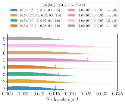
Figure 1: Histograms of posterior samples of the scalar charge inferred by LISA observations of EMRIs with different orbital configurations of central black hole mass $M$ and spin $a$, compact object mass $\mu$, initial eccentricity $e_{0}$ and time to plunge $T$. The colored vertical dashed lines show the one-sided $95\%$ credible interval of the distribution. All EMRI systems are characterized by an SNR of 50.

To forecast the constraints on the scalar charge with EMRI observations we sample over all the intrinsic $\Theta_{i}$ and extrinsic parameters $\Theta_{e}$ of a Kerr equatorial eccentric EMRI signal with scalar charge. We obtain the 13-dimensional posterior distribution using the package Eryn [112], which provides a Bayesian inference tool based on Markov Chain Monte Carlo sampling. The technical details about the likelihood, priors, and sampling techniques are extensively discussed in Appendix C. This is the first appearance of a complete Bayesian parameter inference of EMRI systems in these types of orbits. Moreover, it is the first analysis to include beyond GR corrections that are accurate at adiabatic order.

Results. We consider eight different orbital configurations, specified by their component masses, the primary spin, the initial eccentricity and semi-latus rectum. We assume binaries evolve in the LISA band, plunging over a period $T$. This fixes the initial semi-latus rectum $p_{0}$. For each system, the luminosity distance is fixed to give SNR$=50$.

We first focus on agnostic forecasts of new fundamental fields, assessing LISA’s ability to constrain the scalar charge. To this aim, we study the case in which the injected signal is modelled in GR, i.e., assuming $d=0$, while the recovery template includes the scalar charge. This setup allows us to investigate the upper bound (or constraint) on $d$, which we define as given by the upper 95% credible interval of the corresponding marginalized posterior.

Fig. 1 shows histograms of the marginalized posteriors of the scalar charge for the EMRIs we considered (see Fig. 6 of Appendix C for the full posterior). Bounds on $d$ are tighter for large eccentricity and primary spin. For fixed component masses and evolution time, doubling the eccentricity from $e_{0}=0.2$ to $e_{0}=0.4$ yields a $10\%$ stronger bound on $d$ (cf. systems 6 and 7 in Fig. 1). We find the same level of improvement when increasing the BH spin from $a=0.8$ to $a=0.95$ (systems 5 and 6). However, the precision might vary differently for lower eccentricity binaries, see for instance Fig. 9 of [73].

We also find that increasing the mass ratio provides narrower posteriors. Assuming $\mu=10\,M_{\odot}$, if we reduce the primary mass by a factor of two, we obtain a bound on $d$ that is $\sim 50\%$ tighter (systems $4$ and $6$). This is primarily because a less asymmetric system plunges faster. For a fixed evolution time, such binaries have larger initial orbital separations, where the effect of scalar emission is stronger. To illustrate this point, we analyze a system with component masses $M=10^{5}\,M_{\odot}$ and $\mu=5\,M_{\odot}$ (system 1). This system has the largest initial semi-latus rectum $p_{0}\approx 16$ and, although we consider only the last half a year before the plunge for computational reasons, it yields the best 95% upper bound on $d$, $d_{95\%}=0.015$.

Fixing the intrinsic source parameters, the measurement precision improves for EMRIs evolving over a longer timescale. For a $10^{6}\,M_{\odot}+10\,M_{\odot}$ system, doubling of $T$ improves the constraint on $d$ by $60\%$, and increases the number of cycles from $1.1\times 10^{5}$ to $1.7\times 10^{5}$, and the semi-latus rectum from $p_{0}=8.34$ to $p_{0}=10$.

We now explore the case in which both the injected and the recovery waveforms have a non-vanishing scalar charge. We inject a signal with $d=0.025$, consistent with the upper bound from GW230529 ($d\approx 0.035$), and study constraints on the charge for a $10^{5}M_{\odot}+5M_{\odot}$ EMRI, with the same orbital parameters as system 1 in Fig. 1. This binary provides a measurement of the charge accurate to $\sim 10\%$, with median and 95% credible intervals of $d=0.0244^{+0.006}_{-0.007}$. The marginalized posterior of $d$ for this system is shown in Fig. 2.

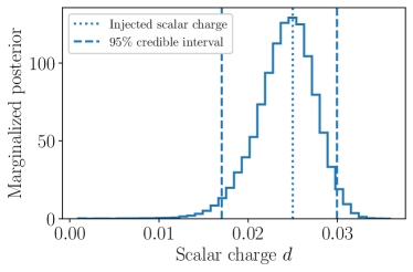
Figure 2: Marginalized posterior distribution of an EMRI system with scalar charge $d=0.025$ and source parameters $M=10^{5}\,M_{\odot}$, $\mu=5\,M_{\odot}$, $a=0.95$, $e_{0}=0.4$, $T=2$ yrs and SNR=50. The estimated median and 95% credible interval are $0.0244^{+0.006}_{-0.007}$.

For the same system, we also explore the impact of ignoring the scalar charge and fitting the data with a GR template (see Appendix F for further details). We find that the GR waveform recovers the injected signal with $2-3\sigma$ biases in the source intrinsic parameters, i.e., its masses and spins. While such systematic errors are large compared to the size of the posterior, they can be considered small for astrophysically motivated studies.

To illustrate how a bound in $d$ can be converted to a constraint on a specific theory, we now consider GB gravity defined by the action in Eq. (8). The forecasted constraints on the coupling constant are shown in Fig. 3. An interesting feature is that the strongest bound for $\sqrt{\alpha}$ comes from system 2, while the strongest bound for $d$ came from system 1. This is because the relation between $d$ and $\alpha$ involves the mass of the secondary.

Selecting a specific theory also allows for a comparison between bounds from EMRIs and bounds from other systems. The analysis of the event GW230529 [7, 113, 114] yielded $\sqrt{\alpha}_{95\%}=1.4\,\rm{km}$, which is a few percent larger than the EMRI constraint obtained with systems 1, 2, and 3. Interestingly, the forecasted best constraint on $\sqrt{\alpha}$ for LVK Voyager is larger (see extremal bound from Figure 21 of [115]). The initial observational frequency of GW230529 is 20 Hz, and the total system mass is $5.1\,M_{\odot}$ and its SNR=11.1 [7]. The dimensionless velocity of GW230529 is $v=(\pi M_{\rm tot}f)^{1/3}\approx 0.117$, whereas the same initial velocity for the lowest total mass EMRI system, $10^{5}\,M_{\odot}+5\,M_{\odot}$, is $v=(\Omega_{\phi})^{1/3}\approx 0.23$. This means that GW230529 is in a weaker field compared to the EMRI systems we considered. In fact, we expect that if we were to consider non-plunging EMRIs with initial dimensionless velocity $v\approx 0.1$ and $p_{0}\approx 60$, the EMRI constraints would further improve. We expect that intermediate-mass ratio inspirals with sufficiently small secondaries can provide even tighter constraints on fundamental fields since their observed inspiral can start in much weaker field regions.

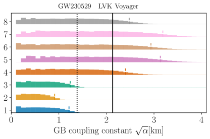
Figure 3: Posterior distribution of the Gauss-Bonnet coupling mapped from the scalar charge constraints (see Fig. 1). The black dotted line in the right panel shows the bound [113] from the observation of the gravitational wave event GW230529 [7], while the black solid line shows the best forecasted bound for LVK Voyager configuration obtained in [115]. We use a different normalization with respect to [113, 115] (see Appendix A).

Discussion. In this work, we produced the first ready-to-use fully relativistic EMRI waveforms in theories of gravity that include a massless scalar field and perform the first Bayesian analysis of EMRI signals in this context. Our waveforms are correct at the adiabatic order and include a single extra parameter, the scalar charge of the EMRI secondary. This is the only parameter needed to capture the effect of the scalar field at this order [51].

Our study provides Bayesian methods and gravitational wave models to investigate the fundamental physics potential of LISA observations of EMRIs. These are two key objectives outlined in the LISA definition study report [16] and the fundamental physics white paper [3]. We also provide an approximate comparison of EMRI constraints on agnostic PN deviations in the phase in Appendix D, where we find that EMRIs provide three orders of magnitude improvement compared to current detectors. The methodologies and findings presented in this paper will play a crucial role in guiding the gravitational wave fundamental physics community.

The main result of our analysis is a forecast of LISA’s ability to measure or place a bound on the scalar charge of the secondary, $d$, in a theory-agnostic manner. This can be interpreted in multiple ways: as a way to look for new fundamental fields; as a way to probe the nature of BHs, by probing the structure of the secondary; and as an indirect test of additional gravitational wave polarizations, as the effects we probe are related to the additional scalar emission.

Bounds on $d$ can be translated to bounds on the coupling constant(s) or a particular theory. We have demonstrated this for a specific example, that of linear-Gauss-Bonnet gravity. Focusing on a specific theory allowed us to compare our forecast with existing bounds and forecasts for the next generation of GW detectors for this particular theory. One of the caveats of this comparison is that our exploration of the parameter space is not exhaustive. As such, it is not clear if the EMRI parameters we have considered are the ones that would yield the most stringent bounds for either $d$ or for the coupling constant of some particular theory. We plan to address this question in future work.

Our waveform model can be extended in several directions. Realistic EMRIs are expected to follow generic, inclined orbits [55]. Studies of EMRIs with new fundamental fields evolving on eccentric and inclined orbits are underway [116]. Inclusion of post-adiabatic corrections, along the lines of Ref. [70], is also essential to include known GR effects that enter at post-adiabatic order, such as the secondary spin [111], and to assess how new fundamental physics can affect the waveform at this order. Our approach can also be generalised to capture massive scalars [54] and more general vector/tensor fields [64].

Acknowledgments. We thank Scott Hughes for providing flux values for comparison with our implementation and Gabriel Andres Piovano for implementing the homogeneous solutions’ functions for the gravitational fluxes computation [117]. This work makes use of the Black Hole Perturbation Toolkit [103]. In particular, the KerrGeodesics [118] and SpinWeightedSpheroidalHarmonics [119] were employed. Some numerical computations have been performed at the Vera cluster supported by MUR and by Sapienza University of Rome. A. Maselli acknowledges financial support from MUR PRIN Grant No. 2022-Z9X4XS, funded by the European Union - Next Generation EU. T.P.S. acknowledges partial support from the STFC Consolidated Grants no. ST/X000672/1 and no. ST/V005596/1. N. Warburton acknowledges support from a Royal Society - Science Foundation Ireland University Research Fellowship. This publication has emanated from research conducted with the financial support of Science Foundation Ireland under grant number 22/RS-URF-R/3825. M. van de Meent acknowledges financial support by the VILLUM Foundation (grant no. VIL37766) and the DNRF Chair program (grant no. DNRF162) by the Danish National Research Foundation. O. Burke acknowledges support from the French space agency CNES in the framework of LISA.

Author Contributions. The Author Contributions statement describes the contributions of individual authors referred to by their initials, and, in doing so, all authors agree to be accountable for the content of the work (see [120] for more information and here for the taxonomy of contributor roles).

LS: Conceptualization, Data Curation, Formal Analysis, Investigation, Methodology, Project Administration, Resources, Software, Supervision, Validation, Visualization, Writing – Original Draft.

SB: Data Curation, Investigation, Resources, Software, Writing - Review & Editing

AM: Conceptualization, Methodology, Writing - Original Draft, Writing - Review & Editing, Supervision, Project Administration.

TPS: Conceptualization, Methodology, Writing - Original Draft, Writing - Review & Editing, Supervision, Project Administration.

NW: Data Curation, Software, Writing - Review & Editing

MvdM: Methodology, Software, Writing - Review & Editing.

AJKC: Conceptualization, Methodology, Writing - Review & Editing.

OB: Investigation, cross-Validation (MCMC & FM studies), Data curation, Writing - Review & Editing

JG: Methodology, Writing - Review & Editing, Supervision.

Appendix A Normalization of the action

We provide here details on the mapping between constraints on the Gauss-Bonnet coupling parameter inferred in this paper and from current and future ground-based detectors.

To compare bounds on the Gauss-Bonnet coupling $\alpha$ we need to take into account the different normalizations considered in the literature for the actions (1) and (8). In particular, constraints derived from current GW observations [121] and by the network of future detectors [115] are obtained by assuming the following action for GB gravity:

$$S=\int d^{4}x\sqrt{-g}\left[\frac{R}{\kappa}-\frac{1}{2}(\nabla\bar{\phi})^{2}+\bar{\alpha}_{\rm GB}\bar{\phi}\mathcal{G}\right]\ ,$$ (11)

where $\kappa=16\pi$. In this paper, we consider instead

$$S=\int d^{4}x\frac{\sqrt{-g}}{\kappa}\left[R-\frac{1}{2}(\nabla\phi)^{2}+\frac{\alpha}{4}\phi\mathcal{G}\right]\ ,$$ (12)

If we scale $\bar{\phi}=\phi\kappa^{-1/2}$ the actions (11) -(12) coincide so long as $\alpha=4\kappa^{1/2}\bar{\alpha}_{\rm GB}$. In our units the constraint available for GB gravity of [121], $\sqrt{\bar{\alpha}_{\rm GB}}\simeq 1.18$ km, translates to $\sqrt{\alpha}=4\pi^{1/4}\sqrt{\bar{\alpha}_{\rm GB}}\simeq 6.3$ km and the constraints from GW230529 $\sqrt{\bar{\alpha}_{\textnormal{GB}}}\simeq 0.260\textnormal{km}\rightarrow\sqrt{\alpha_{\textnormal{GB}}}\simeq 1.4\textnormal{km}$ [113]. Similarly, for the projected bound by LIGO O8, $\sqrt{\bar{\alpha}_{\rm GB}}\simeq 0.4$km (see Fig. 21 of [115]), we obtain$\sqrt{\alpha}\simeq 2.1$km.

The map between the scalar charge and the GB coupling has been obtained in [82], using the action

$$S_{J}=\int\frac{\sqrt{-g}}{\kappa}d^{4}x\left[R-2(\nabla\tilde{\phi})^{2}+\tilde{\alpha}\tilde{\phi}\mathcal{G}\right]\ .$$ (13)

In this setup, at the leading order in $\tilde{\alpha}$, the scalar charge is given by $\tilde{d}=\tilde{\alpha}/(2\mu^{2})$. Passing to the units we use in Eq. (12), $\tilde{d}=d/2$ and $\tilde{\alpha}=\alpha/2$, which leaves the relation $d=d(\alpha)$ unchanged.

Appendix B Flux interpolation

Energy and angular momentum fluxes are interpolated over a three-dimensional grid constructed using 13 Chebyshev-Gauss-Lobatto (CGL) nodes for the eccentricity $e\in[0.0,0.5]$ and the primary spin $a\in[-0.99,0.99]$. Rather than using the semi-latus rectum, we find it more convenient to introduce the variable

$$u=(1+e)\quantity[\frac{\Omega_{\phi}(a,p,e)}{\Omega_{\phi}\left(a,\frac{p_{\rm sep}(a,e)}{1+e},e\right)}]^{2/3}\ ,$$ (14)

where $p_{\rm sep}(a,e)$ is the separatrix for Kerr spacetime, and negative spins correspond to retrograde orbits. We compute $u$ on 17 CGL nodes within $u\in[0.08,0.97]$. Therefore, we calculate scalar and gravitational fluxes on a total of $13\times 13\times 17=2873$ grid points.

Before interpolation, we normalize the fluxes by their leading order contribution in a post-Newtonian expansion. We construct 4 Chebyshev interpolants for the gravitational and scalar energy and angular momentum fluxes. Assuming the fluxes are smooth functions of the variables on our interpolation domain, the accuracy of the Chebyshev interpolation should converge exponentially with the number of grid points. Consequently, we can estimate the interpolation “aliasing” error from the magnitude of the coefficients of the highest order Chebyshev polynomials in each direction. The interpolated quantities and the Chebyshev errors $\sigma$ are shown in Table 1.

If we write the total energy flux as:

$$\dot{E}=\frac{32}{5p^{5}}\quantity(\frac{5p^{5}}{32}\dot{E}_{\rm grav}+\frac{5p^{5}}{32}{d^{2}}\dot{E}_{\rm scal})\ ,$$ (15)

we can estimate the size of the scalar charge that is comparable to the error in the gravitational fluxes

$$\frac{5p^{5}}{32}\dot{E}_{\rm scal}d^{2}>\sigma_{\rm grav}\rightarrow 0.12\,d^{2}>\sigma_{\rm grav}\,,$$ (16)

where we inserted $p^{4}\,\dot{E}_{\rm scal}=0.3$ which is a typical value accross the grid for $p=10$. This gives a relation between the scalar charge and the Chebyshev interpolation. For values of $d=0.01$, we obtain a constraint on the error of the order $10^{-5}$, which is one order of magnitude smaller than what we obtained with our interpolation scheme. This does not invalidate our work, as we treat our interpolated fluxes as the true fluxes and use them consistently for injection and recovery. However, this does highlight the need for denser flux grids and accurate interpolation schemes. The production of dense self-force grids with accurate interpolation methods is a current major challenge for extending the FastEMRIWaveforms package to fully generic orbits in Kerr spacetimes.

Using the Gremlin code for flux calculations evaluated at $a=0.95$, $p=10.1930405906075M$, $e=0.4081632653061225$ we obtain a flux value for $\frac{5}{32}p^{5}\dot{E}_{\text{grav}}$ which differs from our interpolation by absolute and relative errors of $3.8\times 10^{-4},3.6\times 10^{-4}$, respectively. This is compatible within our estimated interpolation error.

Table 1: Chebyshev interpolation of the energy and angular momentum fluxes and the estimates of their absolute interpolation errors.

Interpolated expression	Abs. error
$\frac{5}{32}p^{5}\dot{E}_{\text{grav}}$	$7.5\times 10^{-4}$
$\frac{5}{32}p^{7/2}\dot{L}_{\text{grav}}$	$7.1\times 10^{-4}$
$p^{4}\dot{E}_{\text{scal}}$	$2.3\times 10^{-4}$
$p^{5/2}\dot{L}_{\text{scal}}$	$2.2\times 10^{-4}$

Having the fluxes in hand, we can obtain the right hand side of the Eqns. (9) and then use the FEW package to obtain the EMRI trajectory. As an example, we show in Fig. 4 the trajectories in the $p-e$ plane for binaries with spin $a=0.95$ in GR, i.e., setting the scalar charge to zero, and different EMRI masses. For reference we also show the Chebyshev grid points at the spin $a=0.9562665680261776$.

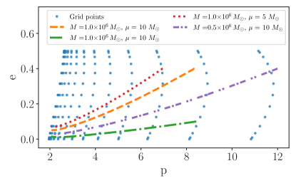
Figure 4: Trajectory evolution of semi-latus rectum and eccentricity for four EMRIs with different component masses and $a=0.95$. For reference, we show the location of the grid points used for interpolation in the $(p,e)$ plane for a constant spin slice at $a=0.9562665680261776$, where the largest value of $p$ reached for this spin is approximately $p\approx 30$.

Appendix C Data analysis setup

The posterior distributions presented in this work are obtained using MCMC sampling with the package Eryn [112, 122]. To run the MCMC, we need to specify the priors $p(\Theta)$ and the likelihood function

$$\ln p(s|\Theta)=\frac{1}{2}\innerproduct{s-h(\Theta)}{s-h(\Theta)}\,,$$ (17)

where we defined the inner product between two GW templates $h_{1}(t)$ and $h_{2}(t)$ [123]:

$$\innerproduct{h_{1}(t)}{h_{2}(t)}=4\real\int_{0}^{\infty}\frac{\tilde{h}_{1}^{*}(f)\tilde{h}_{2}(f)}{S_{n}(f)}\,\differential f\ .$$ (18)

The noise spectral density $S_{n}(f)$ of LISA is taken from [124] and assumed to be known. The tilde denotes the Fourier transform of the waveform and the symbol ^∗ denotes complex conjugation. The Fourier transform and likelihood evaluation are performed on GPUs using cupy [125]. Before passing to the frequency space, we taper $h(t)$ with a Tukey window. The parameter that controls the magnitude of the sinusoidal lobes of the window has been fixed to alpha$=0.005$ [126]. The sampling interval was adjusted for different black hole masses $M$ to avoid aliasing.

The full parameter space of the AAK model is given in Table 2. The response of the detector to the signal is described by the two data channels $h_{I}(t;\Theta)$ and $h_{II}(t;\Theta)$. The full log-likelihood is given by the sum of the log-likelihood for each channel. For reference, we show in Figure 5 the spectrogram of $h_{I}$ for a system with parameters $M=10^{6}\,M_{\odot},\mu=10\,M_{\odot},e_{0}=0.4,d=0.0025,p_{0}=8.3M,T=2\,{\rm yrs}$.

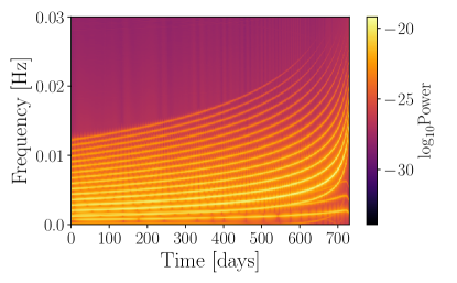
Figure 5: Spectrogram of the gravitational wave signal output of the AAK waveform obtained from an EMRI system with parameters $M=10^{6}\,M_{\odot},\mu=10\,M_{\odot},e_{0}=0.4,d=0.0025,p_{0}=8.3,T=2\,{\rm yrs}$. The different color bands represent the different harmonics, and their color intensity represents their power.

We assume flat priors for all parameters apart from the luminosity distance, which is assumed to follow a power-law distribution with slope $-2$ in the range $[0.01,10.0]$ Gpc. A summary of the priors we consider is given in Table 2. We restrict the prior in $\Phi_{\phi_{0}}$ to $\pi$ and not to $2\pi$ because there is an exact degeneracy every $\pi$. The prior choice of power-law with slope $-2$ for the luminosity distance is motivated by the fact that we found some chains getting stuck at large unphysical values of $d_{L}$. This was caused by chains getting stuck on secondary modes of the likelihood. Our choices allow for better sampling efficiency without affecting the results.

Table 2: Prior distributions on the waveform parameters used for MCMC posterior sampling.

Parameter	Priors ($\delta=0.01$)
$\ln M/M_{\odot}$	Uniform $[\ln M^{*}(1-\delta),\ln M^{*}(1+\delta)]$
$\ln\mu/M_{\odot}$	Uniform $[\ln\mu^{*}(1-\delta),\ln\mu^{*}(1+\delta)]$
$a$	Uniform $[a^{*}(1-\delta),0.98]$
$p_{0}[M]$	Uniform $[p_{0}^{*}(1-\delta),p_{0}^{*}(1+\delta)]$
$e_{0}$	Uniform $[e_{0}^{*}(1-\delta),e_{0}^{*}(1+\delta)]$
$d_{L}$ [Gpc]	Power Law $[0.01,10.0]$
$\cos\theta_{S}$	Uniform $[-0.99999,0.99999]$
$\phi_{S}$	Uniform $[0.0,2\pi]$
$\cos\theta_{K}$	Uniform $[-0.99999,0.99999]$
$\phi_{K}$	Uniform $[0.0,2\pi]$
$\Phi_{\phi_{0}}$	Uniform $[0.0,\pi]$
$\Phi_{r_{0}}$	Uniform $[0.0,2\pi]$
$\Lambda$	Uniform $[-0.6,0.6]$

For parameters that are typically constrained with high precision, i.e., $(M,\mu,a,p_{0},e_{0})$, we center the priors around the true injected values $\Theta_{\rm true}$. In all runs, we find that the posterior support of all parameters is much tighter than the assumed prior.

Since the deviation due to the scalar emission enters the fluxes as $d^{2}$, we sample in the parameter $\Lambda=d^{2}$ with a uniform prior ${\cal U}_{[-0.6,0.6]}$, and then select the samples with $\Lambda>0$. Sampling in $\Lambda$, both positive and negative, allows us to obtain near-Gaussian posteriors, which can be sampled more efficiently with MCMC methods. We verified that this approach does not change the posteriors. We use two proposals to efficiently sample: the stretch move [122] and an adaptive metropolis move that jumps along the eigen-directions of the covariance matrix. We sample the posteriors using 26 walkers, monitoring the integrated autocorrelation time $\tau$ as a function of the iteration. We assume that the estimator for $\tau$ is reliable when it plateaus below the line given by $N_{\text{it}}/50$ for $N_{\text{it}}$ the number of iterations (see this link for further details). We show in the upper corner plot of Figure 6 the full posterior distribution used for the constraints obtained in Figures 1 and 3.

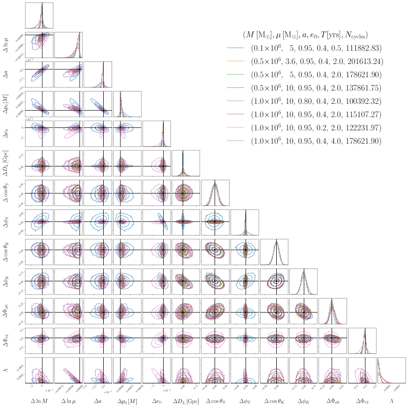
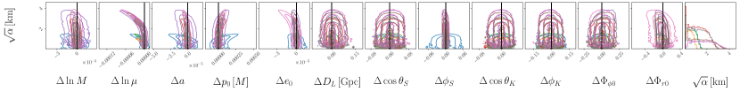
Figure 6: Posterior distribution of EMRI injections with different orbital configurations. The posteriors are centered around the injected parameters. Diagonal and off-diagonal plots provide marginalised and 2D-joint posteriors, respectively. Contour lines in off-diagonal panels identify the 1,2,3$-\sigma$ Gaussian credible contours of each distribution. The upper corner plot shows the posterior distribution output of the MCMC analysis in the parameters of Table 2. The lower corner shows how the list row of the upper corner plot transforms when mapping to the coupling $\sqrt{\alpha}$. In the legend, we provide the system parameters and the number of orbital cycles performed $N_{\rm cycles}$.

To obtain a bound on this specific theory from the posteriors on $\Lambda=d^{2}$ and $\ln\mu$, we use

$$\sqrt{\alpha}=\sqrt{2}\mu\sqrt{d}=\sqrt{2}\,\mu\,\Lambda^{1/4}\,,$$ (19)

and the determinant of the Jacobian of such transformation

$$\differential\sqrt{\alpha}=\quantity|\partialderivative{\sqrt{\alpha}}{\Lambda}|\differential\Lambda\propto\mu\,\Lambda^{-3/4}\differential\Lambda\ .$$ (20)

Similarly, one can obtain the bound on the scalar charge $d$. In the lower corner plot of Figure 6, we can see how the posterior samples are mapped to the coupling $\sqrt{\alpha}$. The posteriors are non-Gaussian and have long tails. This demonstrates the importance of sampling in $\Lambda$ instead of $\sqrt{\alpha}$. Sampling in the latter requires longer iterations to reach convergence and to resolve the tails of the “banana-shaped” distributions.

Appendix D Mapping to agnostic bounds

To compare the potential of EMRIs to constrain deviations from General Relativity for agnostic parametrization, we provide a comparison in terms of the parametrized post-Einsteinian (ppE) formalism or Flexible Theory Independent formalism [13, 127, 128, 129, 130, 131, 132, 133]. We consider the system with $10^{6}\,M_{\odot}+10\,M_{\odot}$ solar masses, initial eccentricity $e_{0}=0.4$, and time to plunge $T=2$ years and run a GR inspiral. We obtain the gravitational energy fluxes $\dot{E}_{\rm grav}$ from the samples obtained, evaluated at the start of the inspiral. If we subtract the median value from this set of samples, and divide by the median, we obtain a set of samples representing the fractional deviation from the expected energy dissipation in GR, that are consistent with the posterior. These can be related to ppE deviations by writing

$$\Delta\dot{E}/\dot{E}_{\rm grav}=Bv^{2n}$$ (21)

where $v=\quantity(\pi\quantity(M+\mu)f)^{1/3}$ with $f$ frequency of the $(l,n_{\phi},n_{r})=(2,2,0)$ and $n$ the post-Newtonian (PN) order. For EMRIs we can approximate $v=\Omega_{\phi}^{1/3}$. The quantity $B$ can be mapped to an “agnostic” deviation in the waveform phase $\delta\varphi$ at different PN orders using the formalism described in [132] (see Eqns. (9)-(11) and (19)-(28) [132] for the mapping $B\rightarrow\delta\varphi$). We provide constraints on $\delta\varphi$ obtained with this procedure as “GR mapping” in Fig. 7. Constraints are $95\%$ upper limits obtained from the posterior on $\delta\varphi$.

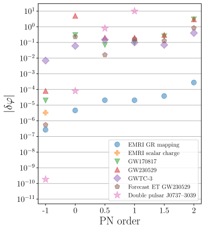
Figure 7: Comparison of the constraints on the phase deviation at different PN orders. The EMRI constraints are obtained from mapping the posterior distribution of a system with parameters $M=10^{6}\,M_{\odot},\mu=10\,M_{\odot},a=0.95,e_{0}=0.4,T=2{\rm yrs}$ and SNR=50 into the phase deviation at different PN orders (blue dots, EMRI GR mapping). For the case of $-1$PN order we use the posterior distribution obtained from an EMRI embedded in a scalar field (orange cross) as done in Figure 1. We show the current constraints obtained from the gravitational wave events GW170817 (down green triangle) [134], GW230529 (up red triangle) [114], and using the GW transient catalogs of the third observing run (GWTC-3) (violet rombo) [4]. Brown pentagon markers correspond to forecasts on $\delta\varphi$ obtained for a GW230529-like binary observed by ET (see main text). The double pulsar constraints obtained from PSR J0737–3039 [135] are shown with pink star markers.

We remark that this analysis is approximate for two reasons. Firstly, post-Newtonian expansions do not provide a good description of the evolution of EMRIs. Secondly, this mapping only considers deviations in the waveforms that can be described by changes in the GR parameters. While any GR deviation causing such a change would definitely not be detectable, larger deviations could also be undetectable, since they are clearly strongly correlated with changes in the EMRI parameters. In that sense, this should be considered an optimistic bound. We note that this method cannot assess the detectability of components of the deviation that change the waveforms in ways that are orthogonal to the GR waveform space, but we expect these to be sub-dominant.

For comparison, we also provide the mapping between the agnostic approach and the scalar charge at the -1PN order, which would correspond to the leading contribution of our full adiabatic scalar emission. In this case, the parameter $B$ is given by [136]:

$$B=d^{2}\,\Omega_{\phi}^{2/3}\dot{E}_{\rm scal}/\dot{E}_{\rm grav}\,.$$ (22)

In Fig. 7, we show the constraints obtained using the GR mapping at different PN orders for the EMRI configuration we considered (blue dots). The scalar charge mapping shows degradation of one order of magnitude (orange cross) at the -1PN order. This demonstrates the importance of correlations that are not taken into account in the GR mapping.

The constraints obtained from the gravitational wave events GW170817 [134], GW230529 [114], and using the GW transient catalogs of the third observing run (GWTC-3) [4] are also shown, and these are a few orders of magnitude larger than the EMRI constraints. This is expected since EMRIs complete $10^{4}-10^{5}$ cycles during the observation, which is two to three orders of magnitude than the number of cycles typically observed in a merger seen by ground-based detectors, leading to correspondingly higher measurement precision. However, better phase constraints do not necessarily imply tighter bounds on the coupling, as this map depends on the specific theory considered. This is the case for GB gravity for which constraints improve for lighter objects, as in the case of GW230529 (see vertical line Fig. 3).

For comparison, we compute bounds on $\delta\varphi$ forecasted for a third-generation ground-based detector like the Einstein Telescope (ET). Constraints are derived through a Fisher matrix approach, analysing the inspiral phase of a binary BH system with the same properties as GW230529 (the source parameters are fixed to the median values reported in [137]). For the analysis, we consider a TaylorF2 waveform model, integrated between 3Hz and the Schwarzschild ISCO. The waveform depends on 7 parameters, $({\cal M},\eta,t_{c},\phi_{c},\chi_{s},\chi_{a},\delta\varphi)$, where ${\cal M}$ and $\eta$ are the chirp mass and the symmetric mass ratio, $(t_{c},\phi_{c})$ the time and phase at the coalescence, $\chi_{s,a}=(\chi_{1}\pm\chi_{2})/2$ combinations of the individual spin components. The phase shift enters the the frequency-domain template as $\tilde{h}(f)=Ae^{i\varphi_{\rm GR(f)}}e^{i\psi(f)}$, where

$$\varphi_{\rm GR}=2\pi ft_{c} -\phi_{c}-\frac{\pi}{4}$$

$$+\frac{3}{128}(\pi{\cal M}f)^{-5/3}\sum_{i=0}^{9}\varphi_{i}(\pi Mf)^{i/3}\ ,$$ (23)

is the GR phase (see Appendix A of [138] for the explicit form of the PN coefficients $\varphi_{i}$) and

$$\psi =\frac{3}{128\eta^{n/5}}\varphi_{n}\delta\varphi_{n}(\pi{\cal M}f)^{(n-5)/3}\quad{\rm if}\quad\varphi_{n}\neq 0\ ,$$ (24)

$$\psi =\frac{3}{128\eta^{n/5}}\delta\varphi_{n}(\pi{\cal M}f)^{(n-5)/3}\quad{\rm if}\quad\varphi_{n}=0\ .$$ (25)

For the Fisher analysis we average over the angles that define the source position in the sky, and consider Gaussian priors on $\chi_{1,2}$, centered around the injected values, and with unit width. Finally we assume for ET a single L-shaped detector with 15 km arm-length [139].

We also show in Fig. 7 the constraint on dipole emission, inferred from observations of the double pulsar PSR J0737–3039 [135]. Such binaries evolve in a low-dynamical regime with $v\approx 2\times 10^{-3}$, and provide the tightest bound on the -1PN phase deviation $\delta\varphi$.

Appendix E Accuracy of the trajectory integration

Gravitational wave observations constrain the frequency evolution of the waveform with great precision. Therefore, it is key to check that the phase evolution is not affected by systematic errors, which could influence the parameter reconstruction. We study the accuracy of the numerical integration of the ordinary differential equations (ODEs) 9. These ODEs are solved using [140] with adaptive step size gsl_odeiv2_step_rk8pd provided by [141].

Firstly, we cross-checked the phase evolution of the implementation against Mathematica on 4 test trajectories. Then, we investigated the difference of the final phase of an inspiral in GR with an ODE absolute error of $10^{-14}$ with respect to the final phase of an inspiral with a given scalar charge $d$ and various different ODE absolute errors. We show the results in Figure 8 for a system with $M=10^{6}\,M_{\odot}$, $\mu=10\,M_{\odot}$, $a=0.95$, $p_{0}=8.343242843079224M$, $e_{0}=0.4$ until its plunge.

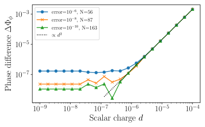
Figure 8: Difference in the final phase between an EMRI evolution obtained with a non-zero scalar charge and various ODE errors (see legend), and an EMRI evolution in GR with an ODE error of $10^{-11}$. For reference, we provide the number of points N taken from the ODE integrator.

For small scalar charges, $d<3\times 10^{-6}$, the phase difference is determined by the ODE solver’s noise floor. On the contrary, the value of the phase difference is independent of the ODE error for large scalar charges $d>3\times 10^{-6}$ and it follows the $d^{2}$ scaling expected by an expansion of the phase difference for small $d$. This expansion is a good approximation up to $d\approx 1$. The ODE error adopted in this work was $5\times 10^{-10}$.

Appendix F Systematic bias due to non-zero scalar charge

In this appendix we provide further details on the systematic bias that could potentially affect EMRI analyses due to the mismatch between a GR recovery template, and a signal with a non-zero scalar charge. This is critical as the charge can influence the binary phase evolution and bias parameter estimation. To investigate such bias we inject an EMRI signal with $d=0.025$ and source parameters $M=10^{5}\,M_{\odot}$, $\mu=5\,M_{\odot}$, $a=0.95$, $e_{0}=0.4$, $T=2$ yrs. We analyse the data with two templates: (i) a GR waveform, and (ii) a waveform model in which the scalar charge is free to vary. The posterior distributions on the EMRI parameters are shown in Fig. 9. We find 2/3 sigma systematic biases in the intrinsic parameters recovered with the GR template. Extrinsic parameters do not present biases larger than 1 sigma and are, therefore, less affected by the waveform mismodeling. The best log-likelihood point obtained with the GR template is $\ln p(s|\Theta)\approx-9$.

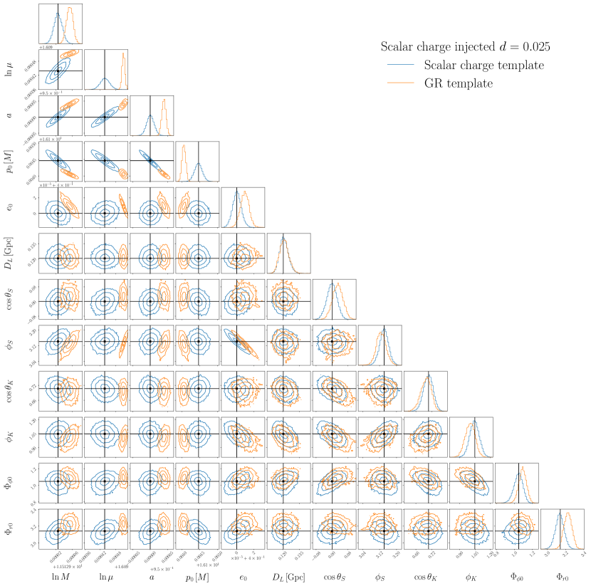
Figure 9: Posterior distribution of an EMRI system with scalar charge $d=0.025$ and source parameters $M=10^{5}\,M_{\odot}$, $\mu=5\,M_{\odot}$, $a=0.95$, $e_{0}=0.4$, $T=2$ yrs and SNR=50. The scalar charge template (blue) correctly recovers the injected parameters, whereas the GR template is biased due to the non-zero scalar charge $d=0.025$.

References

- [1] L. Barack et al., “Black holes, gravitational waves and fundamental physics: a roadmap,” Class. Quant. Grav. 36 no. 14, (2019) 143001, arXiv:1806.05195 [gr-qc].
- [2] E. Barausse et al., “Prospects for Fundamental Physics with LISA,” Gen. Rel. Grav. 52 no. 8, (2020) 81, arXiv:2001.09793 [gr-qc].
- [3] LISA Collaboration, K. G. Arun et al., “New horizons for fundamental physics with LISA,” Living Rev. Rel. 25 no. 1, (2022) 4, arXiv:2205.01597 [gr-qc].
- [4] LIGO Scientific, VIRGO, KAGRA Collaboration, R. Abbott et al., “Tests of General Relativity with GWTC-3,” arXiv:2112.06861 [gr-qc].
- [5] LIGO Scientific, Virgo Collaboration, B. P. Abbott et al., “GW170817: Observation of Gravitational Waves from a Binary Neutron Star Inspiral,” Phys. Rev. Lett. 119 no. 16, (2017) 161101, arXiv:1710.05832 [gr-qc].
- [6] LIGO Scientific, Virgo Collaboration, R. Abbott et al., “GW190412: Observation of a Binary-Black-Hole Coalescence with Asymmetric Masses,” Phys. Rev. D 102 no. 4, (2020) 043015, arXiv:2004.08342 [astro-ph.HE].
- [7] LIGO Scientific, VIRGO, KAGRA Collaboration, “Observation of Gravitational Waves from the Coalescence of a Compact Object and a Neutron Star,” arXiv:2404.04248 [astro-ph.HE].
- [8] LIGO Scientific, Virgo Collaboration, R. Abbott et al., “GW190814: Gravitational Waves from the Coalescence of a 23 Solar Mass Black Hole with a 2.6 Solar Mass Compact Object,” Astrophys. J. Lett. 896 no. 2, (2020) L44, arXiv:2006.12611 [astro-ph.HE].
- [9] M. Punturo et al., “The Einstein Telescope: A third-generation gravitational wave observatory,” Class. Quant. Grav. 27 (2010) 194002.
- [10] S. Dwyer, D. Sigg, S. W. Ballmer, L. Barsotti, N. Mavalvala, and M. Evans, “Gravitational wave detector with cosmological reach,” Phys. Rev. D 91 no. 8, (Apr., 2015) 082001, arXiv:1410.0612 [astro-ph.IM].
- [11] P. Amaro-Seoane et al., “Laser Interferometer Space Antenna,” arXiv e-prints (Feb., 2017) arXiv:1702.00786, arXiv:1702.00786 [astro-ph.IM].
- [12] TianQin Collaboration, J. Mei et al., “The TianQin project: current progress on science and technology,” PTEP 2021 no. 5, (2021) 05A107, arXiv:2008.10332 [gr-qc].
- [13] P. Ajith et al., “The Lunar Gravitational-wave Antenna: Mission Studies and Science Case,” arXiv:2404.09181 [gr-qc].
- [14] B. S. Sathyaprakash et al., “Extreme Gravity and Fundamental Physics,” arXiv:1903.09221 [astro-ph.HE].
- [15] V. Kalogera et al., “The Next Generation Global Gravitational Wave Observatory: The Science Book,” arXiv:2111.06990 [gr-qc].
- [16] M. Colpi et al., “LISA Definition Study Report,” arXiv:2402.07571 [astro-ph.CO].
- [17] L. Barack and C. Cutler, “Using LISA EMRI sources to test off-Kerr deviations in the geometry of massive black holes,” Phys. Rev. D 75 (2007) 042003, arXiv:gr-qc/0612029.
- [18] C. F. Sopuerta and N. Yunes, “Extreme and Intermediate-Mass Ratio Inspirals in Dynamical Chern-Simons Modified Gravity,” Phys. Rev. D 80 (2009) 064006, arXiv:0904.4501 [gr-qc].
- [19] S. Babak, J. Gair, A. Sesana, E. Barausse, C. F. Sopuerta, C. P. L. Berry, E. Berti, P. Amaro-Seoane, A. Petiteau, and A. Klein, “Science with the space-based interferometer LISA. V: Extreme mass-ratio inspirals,” Phys. Rev. D 95 no. 10, (2017) 103012, arXiv:1703.09722 [gr-qc].
- [20] K. Fransen and D. R. Mayerson, “Detecting equatorial symmetry breaking with LISA,” Phys. Rev. D 106 no. 6, (2022) 064035, arXiv:2201.03569 [gr-qc].
- [21] G. Raposo, P. Pani, and R. Emparan, “Exotic compact objects with soft hair,” Phys. Rev. D 99 no. 10, (2019) 104050, arXiv:1812.07615 [gr-qc].
- [22] I. Bena and D. R. Mayerson, “Multipole Ratios: A New Window into Black Holes,” Phys. Rev. Lett. 125 no. 22, (2020) 221602, arXiv:2006.10750 [hep-th].
- [23] M. Bianchi, D. Consoli, A. Grillo, J. F. Morales, P. Pani, and G. Raposo, “Distinguishing fuzzballs from black holes through their multipolar structure,” Phys. Rev. Lett. 125 no. 22, (2020) 221601, arXiv:2007.01743 [hep-th].
- [24] N. Loutrel, R. Brito, A. Maselli, and P. Pani, “Inspiraling compact objects with generic deformations,” Phys. Rev. D 105 no. 12, (2022) 124050, arXiv:2203.01725 [gr-qc].
- [25] G. A. Piovano, A. Maselli, and P. Pani, “Model independent tests of the Kerr bound with extreme mass ratio inspirals,” Phys. Lett. B 811 (2020) 135860, arXiv:2003.08448 [gr-qc].
- [26] P. Pani and A. Maselli, “Love in Extrema Ratio,” Int. J. Mod. Phys. D 28 no. 14, (2019) 1944001, arXiv:1905.03947 [gr-qc].
- [27] G. A. Piovano, A. Maselli, and P. Pani, “Constraining the tidal deformability of supermassive objects with extreme mass ratio inspirals and semianalytical frequency-domain waveforms,” Phys. Rev. D 107 no. 2, (2023) 024021, arXiv:2207.07452 [gr-qc].
- [28] S. Datta, R. Brito, S. Bose, P. Pani, and S. A. Hughes, “Tidal heating as a discriminator for horizons in extreme mass ratio inspirals,” Phys. Rev. D 101 no. 4, (2020) 044004, arXiv:1910.07841 [gr-qc].
- [29] S. Datta and S. Bose, “Probing the nature of central objects in extreme-mass-ratio inspirals with gravitational waves,” Phys. Rev. D 99 no. 8, (2019) 084001, arXiv:1902.01723 [gr-qc].
- [30] E. Maggio, M. van de Meent, and P. Pani, “Extreme mass-ratio inspirals around a spinning horizonless compact object,” Phys. Rev. D 104 no. 10, (2021) 104026, arXiv:2106.07195 [gr-qc].
- [31] P. Pani, E. Berti, V. Cardoso, Y. Chen, and R. Norte, “Gravitational-wave signatures of the absence of an event horizon. II. Extreme mass ratio inspirals in the spacetime of a thin-shell gravastar,” Phys. Rev. D 81 (2010) 084011, arXiv:1001.3031 [gr-qc].
- [32] C. F. B. Macedo, P. Pani, V. Cardoso, and L. C. B. Crispino, “Into the lair: gravitational-wave signatures of dark matter,” Astrophys. J. 774 (2013) 48, arXiv:1302.2646 [gr-qc].
- [33] K. Destounis, F. Angeloni, M. Vaglio, and P. Pani, “Extreme-mass-ratio inspirals into rotating boson stars: Nonintegrability, chaos, and transient resonances,” Phys. Rev. D 108 no. 8, (2023) 084062, arXiv:2305.05691 [gr-qc].
- [34] M. Liu and J.-d. Zhang, “Augmented analytic kludge waveform with quadrupole moment correction,” arXiv:2008.11396 [gr-qc].
- [35] O. Burke, J. R. Gair, J. Simón, and M. C. Edwards, “Constraining the spin parameter of near-extremal black holes using LISA,” Phys. Rev. D 102 no. 12, (2020) 124054, arXiv:2010.05932 [gr-qc].
- [36] M. Rahman and A. Bhattacharyya, “Prospects for determining the nature of the secondaries of extreme mass-ratio inspirals using the spin-induced quadrupole deformation,” Phys. Rev. D 107 no. 2, (2023) 024006, arXiv:2112.13869 [gr-qc].
- [37] A. L. Miller, “Gravitational waves from sub-solar mass primordial black holes,” arXiv:2404.11601 [gr-qc].
- [38] T. Zi, “Extreme mass-ratio inspiral as a probe of extra dimensions: The case of spinning massive object,” Phys. Lett. B 850 (2024) 138538.
- [39] A. Cárdenas-Avendaño and C. F. Sopuerta, “Testing gravity with Extreme-Mass-Ratio Inspirals,” arXiv:2401.08085 [gr-qc].
- [40] T. Zi and P.-C. Li, “Gravitational waves from extreme-mass-ratio inspirals in the semiclassical gravity spacetime,” Phys. Rev. D 109 no. 6, (2024) 064089, arXiv:2311.07279 [gr-qc].
- [41] A. J. K. Chua, S. Hee, W. J. Handley, E. Higson, C. J. Moore, J. R. Gair, M. P. Hobson, and A. N. Lasenby, “Towards a framework for testing general relativity with extreme-mass-ratio-inspiral observations,” Mon. Not. Roy. Astron. Soc. 478 no. 1, (2018) 28–40, arXiv:1803.10210 [gr-qc].
- [42] J. Gair and N. Yunes, “Approximate Waveforms for Extreme-Mass-Ratio Inspirals in Modified Gravity Spacetimes,” Phys. Rev. D 84 (2011) 064016, arXiv:1106.6313 [gr-qc].
- [43] C. Liu, D. Laghi, and N. Tamanini, “Probing modified gravitational-wave propagation with extreme mass-ratio inspirals,” Phys. Rev. D 109 no. 6, (2024) 063521, arXiv:2310.12813 [astro-ph.CO].
- [44] I. D. Saltas and R. Oliveri, “EMRI_MC: A GPU-based code for Bayesian inference of EMRI waveforms,” arXiv:2311.17174 [gr-qc].
- [45] V. Cardoso, S. Chakrabarti, P. Pani, E. Berti, and L. Gualtieri, “Floating and sinking: The Imprint of massive scalars around rotating black holes,” Phys. Rev. Lett. 107 (2011) 241101, arXiv:1109.6021 [gr-qc].
- [46] N. Yunes, P. Pani, and V. Cardoso, “Gravitational Waves from Quasicircular Extreme Mass-Ratio Inspirals as Probes of Scalar-Tensor Theories,” Phys. Rev. D 85 (2012) 102003, arXiv:1112.3351 [gr-qc].
- [47] P. Pani, V. Cardoso, and L. Gualtieri, “Gravitational waves from extreme mass-ratio inspirals in Dynamical Chern-Simons gravity,” Phys. Rev. D 83 (2011) 104048, arXiv:1104.1183 [gr-qc].
- [48] P. Canizares, J. R. Gair, and C. F. Sopuerta, “Testing Chern-Simons Modified Gravity with Gravitational-Wave Detections of Extreme-Mass-Ratio Binaries,” Phys. Rev. D 86 (2012) 044010, arXiv:1205.1253 [gr-qc].
- [49] O. A. Hannuksela, K. W. K. Wong, R. Brito, E. Berti, and T. G. F. Li, “Probing the existence of ultralight bosons with a single gravitational-wave measurement,” Nature Astron. 3 no. 5, (2019) 447–451, arXiv:1804.09659 [astro-ph.HE].
- [50] O. A. Hannuksela, K. C. Y. Ng, and T. G. F. Li, “Extreme dark matter tests with extreme mass ratio inspirals,” Phys. Rev. D 102 no. 10, (2020) 103022, arXiv:1906.11845 [astro-ph.CO].
- [51] A. Maselli, N. Franchini, L. Gualtieri, and T. P. Sotiriou, “Detecting scalar fields with Extreme Mass Ratio Inspirals,” Phys. Rev. Lett. 125 no. 14, (2020) 141101, arXiv:2004.11895 [gr-qc].
- [52] A. Maselli, N. Franchini, L. Gualtieri, T. P. Sotiriou, S. Barsanti, and P. Pani, “Detecting fundamental fields with LISA observations of gravitational waves from extreme mass-ratio inspirals,” Nature Astron. 6 no. 4, (2022) 464–470, arXiv:2106.11325 [gr-qc].
- [53] S. Barsanti, N. Franchini, L. Gualtieri, A. Maselli, and T. P. Sotiriou, “Extreme mass-ratio inspirals as probes of scalar fields: Eccentric equatorial orbits around Kerr black holes,” Phys. Rev. D 106 no. 4, (2022) 044029, arXiv:2203.05003 [gr-qc].
- [54] S. Barsanti, A. Maselli, T. P. Sotiriou, and L. Gualtieri, “Detecting Massive Scalar Fields with Extreme Mass-Ratio Inspirals,” Phys. Rev. Lett. 131 no. 5, (2023) 051401, arXiv:2212.03888 [gr-qc].
- [55] M. Della Rocca, S. Barsanti, L. Gualtieri, and A. Maselli, “Extreme mass-ratio inspirals as probes of scalar fields: inclined circular orbits around Kerr black holes,” arXiv:2401.09542 [gr-qc].
- [56] D. Liang, R. Xu, Z.-F. Mai, and L. Shao, “Probing vector hair of black holes with extreme-mass-ratio inspirals,” Phys. Rev. D 107 no. 4, (2023) 044053, arXiv:2212.09346 [gr-qc].
- [57] C. Zhang, H. Guo, Y. Gong, and B. Wang, “Detecting vector charge with extreme mass ratio inspirals onto Kerr black holes,” JCAP 06 (2023) 020, arXiv:2301.05915 [gr-qc].
- [58] T. Zi, Z. Zhou, H.-T. Wang, P.-C. Li, J.-d. Zhang, and B. Chen, “Analytic kludge waveforms for extreme-mass-ratio inspirals of a charged object around a Kerr-Newman black hole,” Phys. Rev. D 107 no. 2, (2023) 023005, arXiv:2205.00425 [gr-qc].
- [59] J. Lestingi, E. Cannizzaro, and P. Pani, “Extreme mass-ratio inspirals as probes of fundamental dipoles,” arXiv:2310.07772 [gr-qc].
- [60] L. G. Collodel, D. D. Doneva, and S. S. Yazadjiev, “Equatorial extreme-mass-ratio inspirals in Kerr black holes with scalar hair spacetimes,” Phys. Rev. D 105 no. 4, (2022) 044036, arXiv:2108.11658 [gr-qc].
- [61] F. Duque, C. F. B. Macedo, R. Vicente, and V. Cardoso, “Axion Weak Leaks: extreme mass-ratio inspirals in ultra-light dark matter,” arXiv:2312.06767 [gr-qc].
- [62] R. Brito and S. Shah, “Extreme mass-ratio inspirals into black holes surrounded by scalar clouds,” Phys. Rev. D 108 no. 8, (2023) 084019, arXiv:2307.16093 [gr-qc].
- [63] M.-C. Chen, H.-T. Liu, Q.-Y. Zhang, and J. Zhang, “Probing Massive Fields with Multi-Band Gravitational-Wave Observations,” arXiv:2405.11583 [gr-qc].
- [64] S. D. B. Fell, L. Heisenberg, and D. Veske, “Detecting fundamental vector fields with LISA,” Phys. Rev. D 108 no. 8, (2023) 083010, arXiv:2304.14129 [gr-qc].
- [65] L. Speri, A. Antonelli, L. Sberna, S. Babak, E. Barausse, J. R. Gair, and M. L. Katz, “Probing Accretion Physics with Gravitational Waves,” Phys. Rev. X 13 no. 2, (2023) 021035, arXiv:2207.10086 [gr-qc].
- [66] T. P. Sotiriou and S.-Y. Zhou, “Black hole hair in generalized scalar-tensor gravity,” Phys. Rev. Lett. 112 (2014) 251102, arXiv:1312.3622 [gr-qc].
- [67] T. P. Sotiriou and S.-Y. Zhou, “Black hole hair in generalized scalar-tensor gravity: An explicit example,” Phys. Rev. D 90 (2014) 124063, arXiv:1408.1698 [gr-qc].
- [68] F. Thaalba, G. Antoniou, and T. P. Sotiriou, “Black hole minimum size and scalar charge in shift-symmetric theories,” Class. Quant. Grav. 40 no. 15, (2023) 155002, arXiv:2211.05099 [gr-qc].
- [69] M. Saravani and T. P. Sotiriou, “Classification of shift-symmetric Horndeski theories and hairy black holes,” Phys. Rev. D 99 no. 12, (2019) 124004, arXiv:1903.02055 [gr-qc].
- [70] A. Spiers, A. Maselli, and T. P. Sotiriou, “Measuring scalar charge with compact binaries: High accuracy modelling with self-force,” arXiv:2310.02315 [gr-qc].
- [71] N. Warburton, “Self force on a scalar charge in Kerr spacetime: inclined circular orbits,” Phys. Rev. D 91 no. 2, (2015) 024045, arXiv:1408.2885 [gr-qc].
- [72] J. Tan, J.-d. Zhang, H.-M. Fan, and J. Mei, “Constraining the EdGB Theory with Extreme Mass-Ratio Inspirals,” arXiv:2402.05752 [gr-qc].
- [73] C. Zhang, Y. Gong, D. Liang, and B. Wang, “Gravitational waves from eccentric extreme mass-ratio inspirals as probes of scalar fields,” JCAP 06 (2023) 054, arXiv:2210.11121 [gr-qc].
- [74] H. Guo, Y. Liu, C. Zhang, Y. Gong, W.-L. Qian, and R.-H. Yue, “Detection of scalar fields by extreme mass ratio inspirals with a Kerr black hole,” Phys. Rev. D 106 no. 2, (2022) 024047, arXiv:2201.10748 [gr-qc].
- [75] J. E. Chase, “Event horizons in static scalar-vacuum space-times,” Communications in Mathematical Physics 19 no. 4, (Dec., 1970) 276–288.
- [76] J. D. Bekenstein, “Novel “no-scalar-hair” theorem for black holes,” Phys. Rev. D 51 (Jun, 1995) R6608–R6611. https://link.aps.org/doi/10.1103/PhysRevD.51.R6608.
- [77] S. W. Hawking, “Black holes in the brans-dicke,” Communications in Mathematical Physics 25 no. 2, (1972) 167–171. https://doi.org/10.1007/BF01877518.
- [78] L. Capuano, L. Santoni, and E. Barausse, “Black hole hairs in scalar-tensor gravity and the lack thereof,” Phys. Rev. D 108 no. 6, (2023) 064058, arXiv:2304.12750 [gr-qc].
- [79] T. P. Sotiriou and V. Faraoni, “Black holes in scalar-tensor gravity,” Phys. Rev. Lett. 108 (2012) 081103, arXiv:1109.6324 [gr-qc].
- [80] L. Hui and A. Nicolis, “No-Hair Theorem for the Galileon,” Phys. Rev. Lett. 110 (2013) 241104, arXiv:1202.1296 [hep-th].
- [81] R. Nair, S. Perkins, H. O. Silva, and N. Yunes, “Fundamental Physics Implications for Higher-Curvature Theories from Binary Black Hole Signals in the LIGO-Virgo Catalog GWTC-1,” Phys. Rev. Lett. 123 no. 19, (2019) 191101, arXiv:1905.00870 [gr-qc].
- [82] F.-L. Julié and E. Berti, “Post-Newtonian dynamics and black hole thermodynamics in Einstein-scalar-Gauss-Bonnet gravity,” Phys. Rev. D 100 no. 10, (2019) 104061, arXiv:1909.05258 [gr-qc].
- [83] L. Barack and A. Pound, “Self-force and radiation reaction in general relativity,” Rept. Prog. Phys. 82 no. 1, (2019) 016904, arXiv:1805.10385 [gr-qc].
- [84] A. Pound, B. Wardell, N. Warburton, and J. Miller, “Second-Order Self-Force Calculation of Gravitational Binding Energy in Compact Binaries,” Phys. Rev. Lett. 124 no. 2, (2020) 021101, arXiv:1908.07419 [gr-qc].
- [85] N. Warburton, A. Pound, B. Wardell, J. Miller, and L. Durkan, “Gravitational-Wave Energy Flux for Compact Binaries through Second Order in the Mass Ratio,” Phys. Rev. Lett. 127 no. 15, (2021) 151102, arXiv:2107.01298 [gr-qc].
- [86] B. Wardell, A. Pound, N. Warburton, J. Miller, L. Durkan, and A. Le Tiec, “Gravitational Waveforms for Compact Binaries from Second-Order Self-Force Theory,” Phys. Rev. Lett. 130 no. 24, (2023) 241402, arXiv:2112.12265 [gr-qc].
- [87] S. R. Green, S. Hollands, and P. Zimmerman, “Teukolsky formalism for nonlinear Kerr perturbations,” Class. Quant. Grav. 37 no. 7, (2020) 075001, arXiv:1908.09095 [gr-qc].
- [88] S. R. Dolan, C. Kavanagh, and B. Wardell, “Gravitational Perturbations of Rotating Black Holes in Lorenz Gauge,” Phys. Rev. Lett. 128 no. 15, (2022) 151101, arXiv:2108.06344 [gr-qc].
- [89] S. D. Upton and A. Pound, “Second-order gravitational self-force in a highly regular gauge,” Phys. Rev. D 103 no. 12, (2021) 124016, arXiv:2101.11409 [gr-qc].
- [90] V. Toomani, P. Zimmerman, A. Spiers, S. Hollands, A. Pound, and S. R. Green, “New metric reconstruction scheme for gravitational self-force calculations,” Class. Quant. Grav. 39 no. 1, (2022) 015019, arXiv:2108.04273 [gr-qc].
- [91] T. Osburn and N. Nishimura, “New self-force method via elliptic partial differential equations for Kerr inspiral models,” Phys. Rev. D 106 no. 4, (2022) 044056, arXiv:2206.07031 [gr-qc].
- [92] A. Spiers, A. Pound, and J. Moxon, “Second-order Teukolsky formalism in Kerr spacetime: Formulation and nonlinear source,” Phys. Rev. D 108 no. 6, (2023) 064002, arXiv:2305.19332 [gr-qc].
- [93] Z. Nasipak and C. R. Evans, “Resonant self-force effects in extreme-mass-ratio binaries: A scalar model,” Phys. Rev. D 104 no. 8, (2021) 084011, arXiv:2105.15188 [gr-qc].
- [94] G. A. Piovano, A. Maselli, and P. Pani, “Extreme mass ratio inspirals with spinning secondary: a detailed study of equatorial circular motion,” Phys. Rev. D 102 no. 2, (2020) 024041, arXiv:2004.02654 [gr-qc].
- [95] J. Mathews, A. Pound, and B. Wardell, “Self-force calculations with a spinning secondary,” Phys. Rev. D 105 no. 8, (2022) 084031, arXiv:2112.13069 [gr-qc].
- [96] L. V. Drummond and S. A. Hughes, “Precisely computing bound orbits of spinning bodies around black holes. I. General framework and results for nearly equatorial orbits,” Phys. Rev. D 105 no. 12, (2022) 124040, arXiv:2201.13334 [gr-qc].
- [97] S. D. Upton, “Second-order gravitational self-force in a highly regular gauge: Covariant and coordinate punctures,” arXiv:2309.03778 [gr-qc].
- [98] L. V. Drummond, A. G. Hanselman, D. R. Becker, and S. A. Hughes, “Extreme mass-ratio inspiral of a spinning body into a Kerr black hole I: Evolution along generic trajectories,” arXiv:2305.08919 [gr-qc].
- [99] R. Fujita and W. Hikida, “Analytical solutions of bound timelike geodesic orbits in Kerr spacetime,” Class. Quant. Grav. 26 (2009) 135002, arXiv:0906.1420 [gr-qc].
- [100] W. Schmidt, “Celestial mechanics in Kerr space-time,” Class. Quant. Grav. 19 (2002) 2743, arXiv:gr-qc/0202090.
- [101] N. Warburton and L. Barack, “Self force on a scalar charge in Kerr spacetime: circular equatorial orbits,” Phys. Rev. D 81 (2010) 084039, arXiv:1003.1860 [gr-qc].
- [102] “EMRI-scalars repository.” (github.com/susannabarsanti/EMRI-scalars).
- [103] “Black Hole Perturbation Toolkit.” (bhptoolkit.org).
- [104] V. Skoupý and G. Lukes-Gerakopoulos, “Adiabatic equatorial inspirals of a spinning body into a Kerr black hole,” Phys. Rev. D 105 no. 8, (2022) 084033, arXiv:2201.07044 [gr-qc].
- [105] P. Lynch, M. van de Meent, and N. Warburton, “Self-forced inspirals with spin-orbit precession,” arXiv:2305.10533 [gr-qc].
- [106] A. J. K. Chua, C. J. Moore, and J. R. Gair, “Augmented kludge waveforms for detecting extreme-mass-ratio inspirals,” Phys. Rev. D 96 no. 4, (2017) 044005, arXiv:1705.04259 [gr-qc].
- [107] A. J. K. Chua, C. R. Galley, and M. Vallisneri, “Reduced-order modeling with artificial neurons for gravitational-wave inference,” Phys. Rev. Lett. 122 no. 21, (2019) 211101, arXiv:1811.05491 [astro-ph.IM].
- [108] A. J. K. Chua, M. L. Katz, N. Warburton, and S. A. Hughes, “Rapid generation of fully relativistic extreme-mass-ratio-inspiral waveform templates for LISA data analysis,” Phys. Rev. Lett. 126 no. 5, (2021) 051102, arXiv:2008.06071 [gr-qc].
- [109] M. L. Katz, A. J. K. Chua, N. Warburton, and S. A. Hughes., “BlackHolePerturbationToolkit/FastEMRIWaveforms: Official Release,” Aug., 2020. https://doi.org/10.5281/zenodo.4005001.
- [110] M. L. Katz, A. J. K. Chua, L. Speri, N. Warburton, and S. A. Hughes, “Fast extreme-mass-ratio-inspiral waveforms: New tools for millihertz gravitational-wave data analysis,” Phys. Rev. D 104 no. 6, (2021) 064047, arXiv:2104.04582 [gr-qc].
- [111] O. Burke, G. A. Piovano, N. Warburton, P. Lynch, L. Speri, C. Kavanagh, B. Wardell, A. Pound, L. Durkan, and J. Miller, “Accuracy Requirements: Assessing the Importance of First Post-Adiabatic Terms for Small-Mass-Ratio Binaries,” arXiv:2310.08927 [gr-qc].
- [112] N. Karnesis, M. L. Katz, N. Korsakova, J. R. Gair, and N. Stergioulas, “Eryn: a multipurpose sampler for Bayesian inference,” Mon. Not. Roy. Astron. Soc. 526 no. 4, (2023) 4814–4830, arXiv:2303.02164 [astro-ph.IM].
- [113] B. Gao, S.-P. Tang, H.-T. Wang, J. Yan, and Y.-Z. Fan, “Constraints on Einstein-dilation-Gauss-Bonnet Gravity and electric charge of black hole from GW230529,” arXiv:2405.13279 [gr-qc].
- [114] E. M. Sänger et al., “Tests of General Relativity with GW230529: a neutron star merging with a lower mass-gap compact object,” arXiv:2406.03568 [gr-qc].
- [115] S. E. Perkins, N. Yunes, and E. Berti, “Probing Fundamental Physics with Gravitational Waves: The Next Generation,” Phys. Rev. D 103 no. 4, (2021) 044024, arXiv:2010.09010 [gr-qc].
- [116] S. Gliorio et al., “in preparation,”.
- [117] G. A. Piovano, R. Brito, A. Maselli, and P. Pani, “Assessing the detectability of the secondary spin in extreme mass-ratio inspirals with fully relativistic numerical waveforms,” Phys. Rev. D 104 no. 12, (2021) 124019, arXiv:2105.07083 [gr-qc].
- [118] N. Warburton, B. Wardell, O. Long, S. Upton, P. Lynch, Z. Nasipak, and L. C. Stein, “Kerrgeodesics,” July, 2023. https://doi.org/10.5281/zenodo.8108265.
- [119] B. Wardell, N. Warburton, K. Fransen, S. D. Upton, K. Cunningham, A. Ottewill, and M. Casals, “Spinweightedspheroidalharmonics,” May, 2024. https://doi.org/10.5281/zenodo.11199019.
- [120] L. Allen, A. O’Connell, and V. Kiermer, “How can we ensure visibility and diversity in research contributions? how the contributor role taxonomy (credit) is helping the shift from authorship to contributorship,” Learned Publishing 32 (2019) 71–74.
- [121] Z. Lyu, N. Jiang, and K. Yagi, “Constraints on Einstein-dilation-Gauss-Bonnet gravity from black hole-neutron star gravitational wave events,” Phys. Rev. D 105 no. 6, (2022) 064001, arXiv:2201.02543 [gr-qc]. [Erratum: Phys.Rev.D 106, 069901 (2022), Erratum: Phys.Rev.D 106, 069901 (2022)].
- [122] D. Foreman-Mackey, D. W. Hogg, D. Lang, and J. Goodman, “emcee: The MCMC Hammer,” PASP 125 no. 925, (Mar., 2013) 306, arXiv:1202.3665 [astro-ph.IM].
- [123] L. Speri, N. Karnesis, A. I. Renzini, and J. R. Gair, “A roadmap of gravitational wave data analysis,” Nature Astron. 6 no. 12, (2022) 1356–1363.
- [124] S. Babak, A. Petiteau, and M. Hewitson, “LISA Sensitivity and SNR Calculations,” arXiv:2108.01167 [astro-ph.IM].
- [125] R. Okuta, Y. Unno, D. Nishino, S. Hido, and C. Loomis, “Cupy: A numpy-compatible library for nvidia gpu calculations,” in Proceedings of Workshop on Machine Learning Systems (LearningSys) in The Thirty-first Annual Conference on Neural Information Processing Systems (NIPS). 2017. http://learningsys.org/nips17/assets/papers/paper_16.pdf.
- [126] P. Virtanen, R. Gommers, T. E. Oliphant, M. Haberland, T. Reddy, D. Cournapeau, E. Burovski, P. Peterson, W. Weckesser, J. Bright, S. J. van der Walt, M. Brett, J. Wilson, K. J. Millman, N. Mayorov, A. R. J. Nelson, E. Jones, R. Kern, E. Larson, C. J. Carey, İ. Polat, Y. Feng, E. W. Moore, J. VanderPlas, D. Laxalde, J. Perktold, R. Cimrman, I. Henriksen, E. A. Quintero, C. R. Harris, A. M. Archibald, A. H. Ribeiro, F. Pedregosa, P. van Mulbregt, and SciPy 1.0 Contributors, “SciPy 1.0: Fundamental Algorithms for Scientific Computing in Python,” Nature Methods 17 (2020) 261–272.
- [127] C. K. Mishra, K. G. Arun, B. R. Iyer, and B. S. Sathyaprakash, “Parametrized tests of post-Newtonian theory using Advanced LIGO and Einstein Telescope,” Phys. Rev. D 82 (2010) 064010, arXiv:1005.0304 [gr-qc].
- [128] N. Yunes and F. Pretorius, “Fundamental Theoretical Bias in Gravitational Wave Astrophysics and the Parameterized Post-Einsteinian Framework,” Phys. Rev. D 80 (2009) 122003, arXiv:0909.3328 [gr-qc].
- [129] A. Gupta et al., “Possible Causes of False General Relativity Violations in Gravitational Wave Observations,” arXiv:2405.02197 [gr-qc].
- [130] T. G. F. Li, W. Del Pozzo, S. Vitale, C. Van Den Broeck, M. Agathos, J. Veitch, K. Grover, T. Sidery, R. Sturani, and A. Vecchio, “Towards a generic test of the strong field dynamics of general relativity using compact binary coalescence,” Phys. Rev. D 85 (2012) 082003, arXiv:1110.0530 [gr-qc].
- [131] M. Agathos, W. Del Pozzo, T. G. F. Li, C. Van Den Broeck, J. Veitch, and S. Vitale, “TIGER: A data analysis pipeline for testing the strong-field dynamics of general relativity with gravitational wave signals from coalescing compact binaries,” Phys. Rev. D 89 no. 8, (2014) 082001, arXiv:1311.0420 [gr-qc].
- [132] N. Yunes, K. Yagi, and F. Pretorius, “Theoretical Physics Implications of the Binary Black-Hole Mergers GW150914 and GW151226,” Phys. Rev. D 94 no. 8, (2016) 084002, arXiv:1603.08955 [gr-qc].
- [133] A. K. Mehta, A. Buonanno, R. Cotesta, A. Ghosh, N. Sennett, and J. Steinhoff, “Tests of general relativity with gravitational-wave observations using a flexible theory-independent method,” Phys. Rev. D 107 no. 4, (2023) 044020, arXiv:2203.13937 [gr-qc].
- [134] LIGO Scientific, Virgo Collaboration, B. P. Abbott et al., “Tests of General Relativity with GW170817,” Phys. Rev. Lett. 123 no. 1, (2019) 011102, arXiv:1811.00364 [gr-qc].
- [135] M. Kramer et al., “Strong-Field Gravity Tests with the Double Pulsar,” Phys. Rev. X 11 no. 4, (2021) 041050, arXiv:2112.06795 [astro-ph.HE].
- [136] E. Barausse, N. Yunes, and K. Chamberlain, “Theory-Agnostic Constraints on Black-Hole Dipole Radiation with Multiband Gravitational-Wave Astrophysics,” Phys. Rev. Lett. 116 no. 24, (2016) 241104, arXiv:1603.04075 [gr-qc].
- [137] LIGO Scientific, VIRGO, KAGRA Collaboration, A. G. Abac et al., “Observation of Gravitational Waves from the Coalescence of a Compact Object and a Neutron Star,” arXiv:2404.04248 [astro-ph.HE].
- [138] G. Pratten, S. Husa, C. Garcia-Quiros, M. Colleoni, A. Ramos-Buades, H. Estelles, and R. Jaume, “Setting the cornerstone for a family of models for gravitational waves from compact binaries: The dominant harmonic for nonprecessing quasicircular black holes,” Phys. Rev. D 102 no. 6, (2020) 064001, arXiv:2001.11412 [gr-qc].
- [139] M. Branchesi et al., “Science with the Einstein Telescope: a comparison of different designs,” JCAP 07 (2023) 068, arXiv:2303.15923 [gr-qc].
- [140] P. Prince and J. Dormand, “High order embedded runge-kutta formulae,” Journal of Computational and Applied Mathematics 7 no. 1, (1981) 67–75. https://www.sciencedirect.com/science/article/pii/0771050X81900103.
- [141] M. e. a. Galassi, “Gnu scientific library reference manual,” 2018. https://www.gnu.org/software/gsl/.