Equivariance via Minimal Frame Averaging for More Symmetries and Efficiency

Abstract

We consider achieving equivariance in machine learning systems via frame averaging. Current frame averaging methods involve a costly sum over large frames or rely on sampling-based approaches that only yield approximate equivariance. Here, we propose Minimal Frame Averaging (MFA), a mathematical framework for constructing provably minimal frames that are exactly equivariant. The general foundations of MFA also allow us to extend frame averaging to more groups than previously considered, including the Lorentz group for describing symmetries in space-time, and the unitary group for complex-valued domains. Results demonstrate the efficiency and effectiveness of encoding symmetries via MFA across a diverse range of tasks, including $n$-body simulation, top tagging in collider physics, and relaxed energy prediction. Our code is available at https://github.com/divelab/MFA.

1 Introduction

Encoding symmetries in machine learning models has shown impressive results across diverse disciplines, including mathematical problem solving (Puny et al., 2023; Lawrence & Harris, 2023), generalization ability (Kondor & Trivedi, 2018; Gui et al., 2022; Li et al., 2023; Gui et al., 2024), vision (Cohen & Welling, 2016b; Esteves et al., 2020; Worrall & Welling, 2019), quantum mechanics (Unke et al., 2021; Chen et al., 2022; Yu et al., 2023), chemistry (Xu et al., 2021, 2023; Hoogeboom et al., 2022; Batatia et al., 2022; Stärk et al., 2022; Wang et al., 2023a; Fu et al., 2023), materials science (Yan et al., 2022; Lin et al., 2023; Luo et al., 2023; Yan et al., 2024), and physics (Wang et al., 2020, 2022b). Nevertheless, the derivation of equivariant architectures is a non-trivial task and may come at the cost of expressiveness or increased computational effort (Puny et al., 2021; Du et al., 2022; Kim et al., 2023; Duval et al., 2023b; Pozdnyakov & Ceriotti, 2024). Frame averaging (Puny et al., 2021) has emerged as a model-agnostic alternative for instilling equivariance in non-equivariant models. Because the cost of frame averaging operator scales with the size of the frame, sampling-based approaches have been devised to enhance efficiency by sacrificing exact equivariance (Kim et al., 2023; Duval et al., 2023b).

We introduce Minimal Frame Averaging, a mathematical framework for efficient frame averaging that simultaneously maintains exact equivariance. Our general theory also enables us to derive minimal frames for a set of groups strictly larger than those proposed in previous works, including the Lorentz group, the proper Lorentz group, the unitary group, the special unitary group, the general linear group, and the special linear group. Empirically, we demonstrate the advantages of our method on a variety of tasks spanning diverse groups, including $n$-body simulation, isomorphic graph separation, classification of hadronically decaying top quarks (top tagging), relaxed energy prediction on OC20, and prediction of 5-dimenional convex hull volumes.

2 Background

$G$-equivariance of a function $f:\mathcal{V}\to\mathcal{W}$ is defined such that actions from $G$ applied on the domain $\mathcal{V}$ are applied equally to the codomain $\mathcal{W}$. Formally, if $\rho_{\mathcal{W}}$ and $\rho_{\mathcal{V}}$ are representations of $G$ in the spaces $\mathcal{V}$ and $\mathcal{W}$, respectively, then for all $g\in G$ and $x\in\mathcal{V}$,

$$f(\rho_{\mathcal{V}}(g)x)=\rho_{\mathcal{W}}(g)f(x).$$

In the special case where $\rho_{\mathcal{W}}(g)=1$, known as the trivial representation, $f$ is said to be $G$-invariant. Symmetry priors that instill equivariance in neural networks can improve generalization and sample complexity across diverse tasks with exact and approximate symmetries (Bronstein et al., 2021; Han et al., 2022; Zhang et al., 2023). In Section 2.1, we overview prevalent approaches in the sphere of equivariant machine learning before introducing frame averaging in Section 2.2.

2.1 Equivariant Machine Learning

Equivariant methods are largely defined in terms of their choice of internal representation (Duval et al., 2023a; Bronstein et al., 2021; Han et al., 2022). Scalarization methods (Schütt et al., 2018, 2021; Gasteiger et al., 2019, 2021; Köhler et al., 2020; Satorras et al., 2021; Thölke & De Fabritiis, 2021; Jing et al., 2021; Liu et al., 2022; Wang et al., 2022a; Huang et al., 2022; Dym & Gortler, 2024) achieve equivariance by transforming geometric quantities such as vectors into invariant scalars or by manipulating these quantities exclusively by scalar multiplication, and are known to be universal approximators of equivariant functions (Villar et al., 2021; Han et al., 2022). Alternatively, group equivariant CNNs leverage the regular representation, wherein feature maps and kernels are functions on the group $G$ (Cohen & Welling, 2016a; Horie et al., 2021; Wang et al., 2022b, 2023b; Helwig et al., 2023). As this approach requires a feature vector for each group element, it can become prohibitively expensive in cases where the group is large (Bronstein et al., 2021). For $G$ with an infinite number of elements such as the orthogonal group $\mathrm{O}(d)$, network layers may instead map between irreducible representations (Thomas et al., 2018; Weiler et al., 2018; Anderson et al., 2019; Brandstetter et al., 2021; Smidt et al., 2021; Batzner et al., 2022). Although the irreducible approach has been widely used for equivariance to groups such as $\mathrm{O}(d)$, derivation of the irreducible representations for new groups, such as the Lorentz group $\text{O}(1,d-1)$ (Gong et al., 2022), is a non-trivial task (Bronstein et al., 2021). Thus, Ruhe et al. (2023) venture beyond irreducible representations by employing a steerable multivector basis which simultaneously maintains the geometric structure inherent to the data.

2.2 Frame Averaging

While the success of symmetry-preserving frameworks has been demonstrated in a variety of domains and tasks, the construction of equivariant architectures that are both expressive and computationally efficient is challenging (Puny et al., 2021; Du et al., 2022; Kim et al., 2023; Duval et al., 2023b; Kiani et al., 2024). Therefore, Puny et al. (2021) proposed frame averaging, an architecture-agnostic approach to equivariant learning derived from the group averaging operator (Yarotsky, 2022). Group averaging maps an arbitrary function $\Phi:\mathcal{V}\to\mathcal{W}$ to a $G$-equivariant function $\hat{\Phi}$ defined in the case of a finite group $G$ by

$$\hat{\Phi}(x)=\frac{1}{|G|}\sum_{g\in G}\rho_{\mathcal{W}}(g)\Phi(\rho_{\mathcal{V}}(g^{-1})x),$$ (1)

where $|G|$ denotes the cardinality of $G$ and $\rho_{\mathcal{W}}(g)$ as the trivial representation gives a $G$-invariant $\hat{\Phi}$. Computation of Equation 1 quickly becomes intractable as the cardinality of $G$ grows or in the case of an infinite group. Thus, the frame averaging operator replaces $G$ in the summation with a frame $\mathcal{F}(x)\subseteq G$. A special case of interest is a $G$-equivariant frame:

Definition 2.1 ($G$-Equivariant Frame (Puny et al., 2021)).

Given a power set of a finite group $G$ as $\mathcal{P}(G)$, a set-valued function $\mathcal{F}:\mathcal{V}\to\mathcal{P}(G)\setminus\{\emptyset\}$ is termed a $G$-equivariant frame if and only if:

1. $G$-Equivariance: For all $x\in\mathcal{V}$ and $g\in G$, $\mathcal{F}(g\cdot x)=g\mathcal{F}(x)$, where $g\cdot x$ denotes the action of $g$ on $x$;

2. Boundedness: For any $g\in\mathcal{F}(x)$, there exists a constant $c>0$ such that $\|\rho_{\mathcal{W}}(g)\|_{op}\leq c$, where $\|\cdot\|_{op}$ denotes the induced operator norm over $\mathcal{W}$.

By replacing $G$ in Equation 1 with a $G$-equivariant frame $\mathcal{F}$ as

$$\langle\Phi\rangle_{\mathcal{F}}(x)\coloneq\frac{1}{|\mathcal{F}(x)|}\sum_{g\in\mathcal{F}(x)}\rho_{\mathcal{W}}(g)\Phi(\rho_{\mathcal{V}}(g^{-1})x),$$ (2)

the frame averaging operator $\langle\cdot\rangle_{\mathcal{F}}$ achieves equivariance more efficiently than the group averaging operator (Puny et al., 2021). Puny et al. (2021) furthermore leverage the boundedness property in Definition 2.1 to show that the resulting function $\langle\Phi\rangle_{\mathcal{F}}$ maintains the expressivity of the backbone architecture $\Phi$.

3 Methods

In spite of the aforementioned advantages of frame averaging, there are several vital considerations that determine its effectiveness in equivariant learning tasks. First, the efficiency of the frame averaging operator in terms of runtime scales with the size of the frame $\mathcal{F}(x)$. Thus, in Section 3.1, we formalize the concept of a minimal frame and derive a defining property which will enable its computation. Specifically, this property is that the computation of the minimal frame requires a canonical form, which we formalize in Section 3.2. To circumvent challenges that commonly arise when computing the canonical form, we discuss canonicalization on induced $G$-sets in Section 3.3.

Second, the derivation of a $G$-equivariant frame depends directly on the group $G$. Thus, in Section 4, we derive a minimal frame for the linear algebraic group defined by ${\bm{O}}^{T}\eta{\bm{O}}=\eta$, with $\eta$ a diagonal matrix with diagonal entries $\pm 1$. This group subsumes a range of groups which appear frequently in common machine learning tasks, including the orthogonal group $\mathrm{O}(d)$ and the special orthogonal group $\mathrm{SO}(d)$, as well as more specialized groups such as the Lorentz group $\mathrm{O}(1,d-1)$ which describes symmetries of spacetime in particle physics and the unitary group $\mathrm{U}(d)$ describing complex orthogonal matrices. We go on to derive a minimal frame for the permutation group in Section 5, which appears in various graph learning tasks. Beyond these groups, we leverage the mathematical framework developed in Sections 3.1, 3.2 and 3.3 to derive minimal frame averaging for a variety of groups in Appendix H, including $\mathbb{R}^{d},\mathrm{E}(d),\mathrm{SE}(d),\mathrm{GL}(d,\mathbb{R}),$ and $\mathrm{SL}(d,\mathbb{R})$.

3.1 Construction of the Minimal Frame

To more precisely define a frame with minimal size, we introduce the concept of a minimal frame defined on a $G$-set $\mathcal{S}$.

Definition 3.1 (Minimal Frame).

A minimal frame $\hat{\mathcal{F}}:\mathcal{S}\rightarrow\mathcal{P}(G)\setminus\{\emptyset\}$ is a frame such that for any $x\in\mathcal{S}$, there does not exist a frame $\mathcal{F}$ with $\mathcal{F}(x)\subset\hat{\mathcal{F}}(x)$.

The following result, proven in Section B.2, relates an arbitrary frame $\mathcal{F}$ to the stabilizer of an element of interest $x_{0}$ residing in the orbit of $x$. The stabilizer of $x_{0}$ is defined as $\text{Stab}_{G}\left(x_{0}\right)\coloneq\{g\in G\mid g\cdot x_{0}=x_{0}\}$, while the orbit of $x$ is defined as ${\text{Orb}_{G}\left(x\right)\coloneq\{g\cdot x\mid g\in G\}}$. This result will prove vital in constructing minimal frames.

Lemma 3.1.

Given a frame $\mathcal{F}:\mathcal{S}\rightarrow\mathcal{P}(G)\setminus\{\emptyset\}$, for all $x\in\mathcal{S}$, there exists $x_{0}\in\text{Orb}_{G}(x)$ such that $\text{Stab}_{G}(x_{0})\subseteq\mathcal{F}(x_{0})$.

Using this result, we next show that for each $x\in\mathcal{S}$, $\hat{\mathcal{F}}(x)$ may be derived by selecting a unique representative $x_{0}\in\text{Orb}_{G}\left(x\right)$ and computing its stabilizer, the proof of which can be found in Section B.3. We refer to $x_{0}=c(x)$ as the canonical form with the canonicalization function $c$, and its uniqueness is in the sense that all elements in $\text{Orb}_{G}\left(x\right)$ share the same canonical form. We discuss the canonical form in greater detail in Section 3.2 where we find that identifying a canonical form can be non-trivial depending on the group $G$ and base space $\mathcal{S}$, although for the purposes of a general derivation of the minimal frame in the following result, we simply assume that we have access to it.

Theorem 3.2.

For all $x\in\mathcal{S}$, let ${\color[rgb]{0,0,0}x_{0}=c(x)=h^{-1}\cdot x}$ for some $h\in G$. Define the frame $\mathcal{F}:\mathcal{S}\rightarrow\mathcal{P}(G)\setminus\{\emptyset\}$ such that $\mathcal{F}(x)=h\text{Stab}_{G}(x_{0})$; then, $\mathcal{F}$ is a minimal frame.

This result shows how a minimal frame $\hat{\mathcal{F}}(x)$ is constructed through the canonical form $x_{0}$ such that $\hat{\mathcal{F}}(x)=h\text{Stab}_{G}\left(x_{0}\right)$, and is a generalization of Theorem 3 from Puny et al. (2021), which shows that $\lvert\mathcal{F}(x)\rvert\geq\lvert\text{Stab}_{G}\left(x\right)\rvert$ given any equivariant frame $\mathcal{F}$ for invariant frame averaging. However, there are cases where $\lvert\text{Stab}_{G}\left(x\right)\rvert$ is infinite, e.g., a point cloud lying on a $(d-2)$-dimensional Euclidean subspace embedded in a $d$-dimensional Euclidean space under the action of $\mathrm{O}(d)$. While it then appears natural to define the minimal frame in terms of a measure on the group $\mu$, the existence of sets with measure 0 imply that Definition 3.1 is stronger. Specifically, we might instead define the minimal frame $\hat{\mathcal{F}}$ such that for all $x$ and equivariant frames $\mathcal{F}$, $\mu(\hat{\mathcal{F}}(x))\leq\mu(\mathcal{F}(x))$. It would then follow that for the set $A(x)\subset G$ such that $A(x)\cap\hat{\mathcal{F}}(x)\neq\emptyset$ and $\mu(A(x))=0$, the frame $\tilde{\mathcal{F}}(x)\coloneq\hat{\mathcal{F}}(x)\cup A(x)$ is also minimal, as $\mu(\tilde{\mathcal{F}}(x))=\mu(\hat{\mathcal{F}}(x))$, whereas $\tilde{\mathcal{F}}$ is not minimal by Definition 3.1 since $\hat{\mathcal{F}}(x)$ is a proper subset of $\tilde{\mathcal{F}}(x)$. However, as proven in Theorem D.5, minimality in terms of any measure is implied by Definition 3.1, and thus, Definition 3.1 is stronger.

3.2 The Canonical Form

Equipped with a notion of the minimal frame and how it is constructed using a canonical form $c(x)\coloneq x_{0}$, we now formalize $c(x)$ by generalizing the definition of McKay & Piperno (2014) beyond graphs, and discuss canonicalization in 2 concrete cases.

Definition 3.3 (Canonical Form).

Given an equivalence relation $\sim$ on $\mathcal{S}$ such that for any $x,y\in\mathcal{S}$, $x\sim y$ if and only if $y\in\text{Orb}_{G}\left(x\right)$, a canonicalization with respect to $\sim$ is a mapping $c:\mathcal{S}\rightarrow\mathcal{S}$ satisfying the following conditions for all $x,y\in\mathcal{S}$:

1. Representativeness: $x\sim c(x)$;

2. $G$-invariance/ Uniqueness: $c(x)=c(y)$ if $x\sim y$.

Property 1 in Definition 3.3 requires that the canonical form is a single element residing in the orbit of $x$, while Property 2 requires that the canonical form be unique within each orbit. An example of canonicalization is of a symmetric matrix ${\bm{P}}\in\mathbb{R}^{d\times d}$, where the orthogonal group $\mathrm{O}(d)$ acts by conjugate multiplication. Given the eigendecomposition ${\bm{P}}={\bm{O}}^{T}{\bm{\Lambda}}{\bm{O}}$ with eigenvalues ${\bm{\Lambda}}$ in an ascending/descending order, $c({\bm{P}})={\bm{\Lambda}}$ is a valid canonical form, as ${\bm{\Lambda}}$ is uniquely defined and invariant to actions of $\mathrm{O}(d)$ on ${\bm{P}}$, and furthermore, ${\bm{\Lambda}}\in\mathrm{Orb}_{\mathrm{O}(d)}({\bm{P}})$.

In many cases, canonicalization may be elusive. For example, consider the canonicalization of ${\bm{P}}\in\mathbb{R}^{d\times n}$ where the orthogonal group instead acts by left multiplication. From Theorem 3.2, we must decompose ${\bm{P}}=\rho(g){\bm{R}}$ for $g\in\mathrm{O}(d)$, $\rho(g)\in\mathbb{R}^{d\times d}$, and ${\bm{R}}\in\mathbb{R}^{d\times n}$ as the canonical form. This may be achieved by a QR decomposition of ${\bm{P}}$, however, if ${\bm{P}}$ does not have full column rank, ${\bm{R}}$ will not be uniquely defined. This non-uniqueness raises issues in ensuring that the canonical form satisfies the $\mathrm{O}(d)$-invariance required by Definition 3.3. In the following section, we resolve such cases by demonstrating how canonicalization can instead be performed on an induced $G$-set to achieve a unique canonical form.

3.3 Frame Construction on Induced $G$-Sets

As in the previous example of $\mathrm{O}(d)$ acting upon non-full column rank matrices via left multiplication, there are cases in which practical attempts at deriving a canonical form instead give rise to a set of multiple candidates. In order to satisfy $G$-invariance, a candidate must be selected in a manner so as to preserve the uniqueness of the canonical form within $\text{Orb}_{G}\left(x\right)$. To do so, we introduce a $G$-equivariant function $\phi$ to remove the ambiguity, and instead compute the canonical form of $\phi(x)$ in a space $\mathcal{S}_{\phi}$ which we refer to as an induced $G$-set.

Definition 3.4 (Induced $G$-set).

An induced $G$-set $\mathcal{S}_{\phi}$ is a $G$-set induced from the $G$-set $\mathcal{S}$ through a $G$-equivariant function $\phi:\mathcal{S}\rightarrow\mathcal{S}_{\phi}$ such that for all $g\in G$ and $x\in\mathcal{S}$, $\phi(g\cdot x)=g\cdot\phi(x)$.

A well-chosen $\phi$ can effectively remove ambiguity in the canonical form by computing the canonical form on $\mathcal{S}_{\phi}$ instead of on the original space $\mathcal{S}$, however, it is unclear how this will be useful for deriving a minimal frame on $\mathcal{S}$. As we state next and prove in Section B.4, due to the $G$-equivariance of $\phi$, $\phi$ may be composed with a frame $\mathcal{F}_{\phi}$ on $\mathcal{S}_{\phi}$ to produce a frame on $\mathcal{S}$, although we note that this frame is not necessarily minimal.

Theorem 3.5.

Given a $G$-set $\mathcal{S}$ and a $G$-equivariant function $\phi:\mathcal{S}\rightarrow\mathcal{S}_{\phi}$, let $\mathcal{F}_{\phi}:\mathcal{S}_{\phi}\rightarrow\mathcal{P}(G)\setminus\{\emptyset\}$ be a frame with the domain of $\mathcal{S}_{\phi}$. Then, $\mathcal{F}_{\phi}\circ\phi$ is a frame with the domain of $\mathcal{S}$.

Interestingly, previous methods can be shown to be special cases of canonicalization on an induced $G$-set. For example, for $\phi({\bm{P}})={\bm{P}}{\bm{P}}^{T}$, the canonical form $c(\phi({\bm{P}}))$ is given by eigenvalues of $\phi({\bm{P}})$, which is exactly the method of Puny et al. (2021). Additionally, choosing the trivial map $\phi({\bm{P}})=0$ gives the minimal frame $\hat{\mathcal{F}}_{\phi}(\phi({\bm{P}}))=G$ which corresponds to group averaging, as $c(\phi({\bm{P}}))=0$ and $\text{Stab}_{G}\left(0\right)=G$. This illustrates that canonicalization can be more tractable on the induced $G$-set, though it is not necessarily the case that a minimal frame $\hat{\mathcal{F}}_{\phi}$ on the induced $G$-set produces a frame $\hat{\mathcal{F}}_{\phi}\circ\phi$ which is also minimal on the base space.

We next derive minimal frames for several groups acting on subsets of $\mathbb{R}^{d\times n}$. In Section 4, we employ an induced $G$-set to derive a minimal frame for the linear algebraic group $G_{\eta}(d)$, which is strictly more general than the previously mentioned example of $\mathrm{O}(d)$. In Section 5, we go on to consider a case where the minimal frame can be directly computed on $\mathcal{S}$ for the permutation group $\text{S}_{n}$. Furthermore, in Table 8, we present induced $G$-sets which we leverage to compute canonical forms for a variety of groups and domains.

4 Linear Algebraic Group

The linear algebraic group $G_{\eta}(d)$ includes several well-known groups: the orthogonal group $\mathrm{O}(d)$, the Lorentz group $\text{O}(1,d-1)$ and the unitary group $\mathrm{U}(d)$. By adding a constraint enforcing determinant equal to 1, $G_{\eta}(d)$ can be extended to include groups like $\mathrm{SO}(d),\mathrm{SO}(1,d-1)$ and $\mathrm{SU}(d)$. $G_{\eta}(d)$ acts on ${\bm{x}}\in\mathbb{R}^{d}$ as $g\cdot{\bm{x}}\coloneq{\bm{O}}{\bm{x}}$, where $\rho(g)={\bm{O}}\in\mathbb{R}^{n\times n}$ satisfies ${\bm{O}}^{T}\eta{\bm{O}}=\eta$, and $\eta$ is a $d\times d$ diagonal matrix with diagonal elements $\pm 1$. The pseudo-inner product on $\mathbb{R}^{d}$ is then defined by $\langle{\bm{x}},{\bm{y}}\rangle\coloneqq{\bm{x}}^{T}\eta{\bm{y}}$. Setting $\eta={\bm{I}}_{d}$ results in $G_{\eta}(d)=\mathrm{O}(d)$ with the usual Euclidean inner product. However, as we aim to develop theory that goes beyond $\mathrm{O}(d)$, we encounter $\eta\neq{\bm{I}}_{d}$, resulting in non-Euclidean, pseudo-inner products. For example, setting $\eta=\text{diag}(1,-1,\cdots,-1)\in\mathbb{R}^{d\times d}$ gives $G_{\eta}(d)=\mathrm{O}(1,d-1)$, the Lorentz Group. This generality introduces a multitude of challenges that lead us to define MFA frames on an induced $G_{\eta}(d)$-set in Section 4.1 and to develop a generalized QR decomposition for canonicalization in Section 4.2 before moving on to derive minimality and an efficient closed form of the frame averaging operator in Section 4.3. Furthermore, to encompass the case of $G_{\eta}(d)$ acting on $\mathbb{C}^{d}$, MFA is extended to unitary groups in Section 4.5.

4.1 Canonicalization on the Induced $G_{\mathbf{\eta}}(d)$-Set

We aim to construct a $G_{\eta}(d)$-equivariant map by applying the frame averaging operator over a frame $\hat{\mathcal{F}}({\bm{P}})$, where ${\bm{P}}\in\mathbb{R}^{d\times n}$ represents a collection of $n$ elements of $\mathbb{R}^{d}$. From Theorem 3.2, construction of $\hat{\mathcal{F}}$ requires a canonical form $\hat{{\bm{R}}}=\hat{{\bm{Q}}}^{-1}{\bm{P}}$ for $\rho^{-1}({\bm{Q}})\in G_{\eta}(d)$, where $\rho$ is the group representation. While the QR decomposition can be applied as ${\bm{P}}={\bm{Q}}{\bm{R}}$, ${\bm{R}}$ will only be unique in the case where ${\bm{P}}$ has full column rank, which is necessary to satisfy the $G_{\eta}(d)$-invariance required by Definition 3.3. Furthermore, the QR decomposition involves a division by $\langle{\bm{v}}_{1},{\bm{v}}_{1}\rangle$ for the first chosen columns ${\bm{v}}_{1}$ of ${\bm{P}}$. This may result in division by zero, as due to the non-Euclidean inner product, $\langle{\bm{v}}_{1},{\bm{v}}_{1}\rangle$ may be $0$ even for ${\bm{v}}_{1}\neq\mathbf{0}\in\mathbb{R}^{d}$, in which case we refer to ${\bm{v}}_{1}$ as null.

For these reasons, we transform ${\bm{P}}$ to an induced $G_{\eta}(d)$-set through the map $\phi$ which selects columns of ${\bm{P}}$ such that $\phi({\bm{P}})\in\mathbb{R}^{d\times d^{\prime}}$ has full column rank and no null columns. Note that this selection is equivariant as required by Definition 3.4, as $G_{\eta}(d)$ acts via left multiplication of ${\bm{P}}$ and the selection is implemented as right multiplication with ${\bm{M}}\in\mathbb{R}^{d\times d^{\prime}}$ as $\phi({\bm{P}})={\bm{P}}{\bm{M}}$. ${\bm{M}}$ is constructed by removing the $j$-th column from ${\bm{I}}_{d}$ if and only if the $j$-th column is null or is linearly dependent with respect to the other non-null vectors. Note that when considering $\mathrm{SO}(d)$ and ${\bm{M}}$ constructed so as to select three vectors within every local two-body system, the methods proposed by Du et al. (2022) and Pozdnyakov & Ceriotti (2024) can be seen as special cases of the approach we have taken here.

4.2 Derivation of the Canonical Form via Generalized QR Decomposition

Despite these considerations, there are still several obstacles preventing the computation of $\hat{\bm{Q}}$ and $\hat{\bm{R}}$ directly from the QR decomposition of $\phi({\bm{P}})={\bm{Q}}{\bm{R}}$, and we therefore develop a generalized QR decomposition which allows us to derive minimal frames for $G_{\eta}(d)$. First, there may not be $\hat{g}\in G_{\eta}(d)$ such that $\rho(\hat{g})={\bm{Q}}$, as ${\bm{Q}}^{T}\eta{\bm{Q}}$ may not result in $\eta$, and instead give ${\bm{S}}\eta{\bm{S}}^{T}$, where ${\bm{S}}$ is a permutation matrix. This is due to the negativity of the pseudo-inner product and the sequential nature with which the QR decomposition computes the columns of ${\bm{Q}}$ via the Gram-Schmidt process. For example, consider $G_{\eta}(d)=\mathrm{O}(1,d-1)$ with $\eta=\text{diag}(1,-1,\cdots,-1)$. The first vector ${\bm{v}}_{1}$ used for the Gram-Schmidt process could be time-like, i.e., $\langle{\bm{v}}_{1},{\bm{v}}_{1}\rangle<0$, such that the first element of ${\bm{Q}}^{T}\eta{\bm{Q}}$ is $-1$ instead of $1$. To counteract this, we introduce ${\bm{S}}$ into our generalized QR decomposition as $\hat{{\bm{Q}}}\coloneq{\bm{Q}}{{\bm{S}}}$ such that $\hat{{\bm{Q}}}^{T}\eta\hat{{\bm{Q}}}=\eta$. Additionally, $\det({\bm{Q}})=\pm 1$ because the QR decomposition results in an orthonormal ${\bm{Q}}$, however, groups of $G_{\eta}(d)$ with additional determinant constraints such as $\mathrm{SO}(d)$ and $\mathrm{SO}(1,d-1)$ require that $\det({\bm{Q}})=1$. For these groups, we flip the sign of the elements in one of the columns of $\hat{\bm{Q}}$ if $\det({\bm{Q}})=-1$, which we detail further in Section H.2. These steps have ensured that there exists $\hat{g}\in G_{\eta}(d)$ such that $\rho(\hat{g})=\hat{{\bm{Q}}}$.

Second, the classical QR decomposition may not even be a valid decomposition of $\phi({\bm{P}})$, that is, $\phi({\bm{P}})\neq{\bm{Q}}{\bm{R}}$. This is due to division by the $L_{2}$-norm $\lVert{\bm{u}}\rVert$ in the computation of the QR decomposition detailed in Section E.1, where ${\bm{u}}$ is an intermediate vector used in the Gram-Schmidt process. While the standard definition of $\lVert{\bm{u}}\rVert$ is $\sqrt{\langle{\bm{u}},{\bm{u}}\rangle}$, the pseudo-inner product may result in $\langle{\bm{u}},{\bm{u}}\rangle<0$. Redefining $\lVert{\bm{u}}\rVert$ as $\sqrt{\lvert\langle{\bm{u}},{\bm{u}}\rangle\rvert}$ circumvents a complex-valued norm, however, it also invalidates the decomposition. We therefore define $\hat{{\bm{R}}}\coloneqq{\bm{S}}^{T}{\bm{D}}_{\eta}{\bm{R}}$, where both ${\bm{S}}^{T}$ and ${\bm{D}}_{\eta}$ serve to ensure $\hat{{\bm{Q}}}\hat{{\bm{R}}}$ is a valid decomposition of $\phi({\bm{P}})$. ${\bm{S}}^{T}$ cancels ${\bm{S}}$ in $\hat{\bm{Q}}$, while ${\bm{D}}_{\eta}$ is a diagonal matrix with diagonal elements $({\bm{D}}_{\eta})_{j,j}\coloneq{\color[rgb]{0,0,0}\operatorname{sign}(\langle{\bm{u}}_{j},{\bm{u}}_{j}\rangle)}$. The above steps have ensured that $\phi({\bm{P}})=\hat{{\bm{Q}}}\hat{{\bm{R}}}$ with $\hat{{\bm{Q}}}^{T}\eta\hat{{\bm{Q}}}=\eta$. In Section E.1, we further show the uniqueness of $\hat{{\bm{R}}}$, ensuring that $\hat{{\bm{R}}}$ is a valid canonical form.

4.3 Minimal Frame Averaging on $G_{\eta}(d)$

As discussed in Section 3.3, since $\hat{\bm{R}}$ was computed on an induced $G_{\eta}(d)$-set, it is not necessarily the case that frames derived from $\hat{\bm{R}}$ will be minimal on the base space $\mathbb{R}^{d\times n}$. In the proof of the following result in Section B.6, we prove this base space minimality by leveraging Theorems 3.2 and 3.5.

Theorem 4.1.

Let $\hat{\mathcal{F}}_{\phi}$ be a minimal frame on the $G_{\eta}(d)$-set induced by $\phi({\bm{P}})={\bm{P}}{\bm{M}}$ computed via the generalized QR decomposition; if the columns of ${\bm{P}}$ are non-null, then $\hat{\mathcal{F}}_{\phi}\circ\phi$ is a minimal frame on the original domain $\mathbb{R}^{d\times n}$.

Finally, we discuss practical computation of the frame averaging operator over $\hat{\mathcal{F}}_{\phi}\circ\phi$. Theorem 3.2 implies that we must next compute $\textrm{Stab}_{G_{\eta}(d)}(\hat{{\bm{R}}})$, which is indeed the route we will take when $d^{\prime}=d$. However, when $d^{\prime}<d$, there are infinite $\hat{{\bm{Q}}}$ satisfying $\phi({\bm{P}})=\hat{{\bm{Q}}}\hat{{\bm{R}}}$, apparently making the operator intractable. We therefore employ an alternate form of the minimal frame given in Lemma B.1 which we prove to be equivalent to the form established by Theorem 3.2. This alternate form enables us to derive an efficient closed form of the operator shown in the following result, the proof of which is given in Section B.7.

Theorem 4.2.

Let $\hat{{\bm{Q}}},\hat{{\bm{R}}}$ be computed via the generalized QR decomposition such that $\phi({\bm{P}})=\hat{{\bm{Q}}}\hat{{\bm{R}}}\in\mathbb{R}^{d\times d^{\prime}}$, and assume that the columns of ${\bm{P}}$ are non-null. Then, there exists ${\bm{Q}}_{0}\in\mathbb{R}^{d\times d}$ such that the frame averaging operator applied to an arbitrary function ${\color[rgb]{0,0,0}\Phi}:\mathbb{R}^{d\times n}\rightarrow\mathbb{R}^{d\times n}$ over the minimal frame $\hat{\mathcal{F}}_{\phi}\circ\phi$ is given by

$${\color[rgb]{0,0,0}\langle\Phi\rangle_{\hat{\mathcal{F}}_{\phi}\circ\phi}({\bm{P}})}={\bm{Q}}_{0}\Phi\left(\hat{{\bm{Q}}}^{-1}{\bm{P}}\right),$$

where $d^{\prime}$ columns of ${\bm{Q}}_{0}$ are obtained directly from $\hat{{\bm{Q}}}$, and the remaining $d-d^{\prime}$ columns are all $\mathbf{0}\in\mathbb{R}^{d}$.

4.4 Efficiency compared to Puny et al. (2021).

Puny et al. (2021) consider $\mathrm{O}(d)$ and $\mathrm{SO}(d)$. Their method is equivalent to employing the induced $G$-set $\phi({\bm{P}})={\bm{P}}{\bm{P}}^{T}$ and performing canonicalization via the eigendecomposition, which cannot be used for groups such as $\mathrm{O}(1,d-1)$. Furthermore, for a full column rank non-degenerate (i.e., no eigenvalues are repeated) matrix ${\bm{P}}$, the size of their frame is $2^{d}$, while the generalized QR decomposition is unique for both $\hat{\bm{Q}}$ and $\hat{\bm{R}}$ by Theorem E.1, producing a frame with only $1$ element. Additionally, the size of the frame obtained from the generalized QR decomposition remains 1 in the case of a full column rank degenerate ${\bm{P}}$, however, relying on the eigendecomposition of ${\bm{P}}{\bm{P}}^{T}$ in such a setting will produce a frame of infinite size. In Section H.3, we provide an eigenvalue perturbation method to solve this degenerate case for the method of Puny et al. (2021). However, the size of the resulting frame is still $2^{d}$, which is larger than the frame produced by the MFA method.

4.5 Complex domain

The extension from the real vector space $\mathbb{R}^{d\times n}$ to a complex vector space $\mathbb{C}^{d\times n}$ is natural. By changing all the transpose operations ${\bm{Q}}^{T}$ to the conjugate transpose operations ${\bm{Q}}^{*}$ and inner products to conjugate inner products, the generalized QR decomposition is conducted as in the real space for the unitary group $\mathrm{U}(d)$. For $\mathrm{SU}(d)$, we require that the magnitude of $\det(\hat{{\bm{Q}}})\in\mathbb{C}$ be $1$. This constraint is satisfied through a scaling $\det({\bm{Q}})^{-1/d}$ and its inverse applied to $\hat{{\bm{Q}}}$ and $\hat{{\bm{R}}}$, respectively.

5 Permutation Group

We now consider minimal frames for two different spaces under the action of the permutation group $\mathrm{S}_{n}$ beginning with the space of undirected graphs in Section 5.1. Using the results from Section 5.1, we go on to derive minimal frames for point clouds acted upon by the group formed from the direct product of $\mathrm{S}_{n}$ and $G_{\eta}(d)$ in Section 5.3 under the assumption that we already possess an $G_{\eta}(d)$-invariant/equivariant backbone model.

5.1 Minimal Frame for Undirected Graphs

$\mathrm{S}_{n}$ acts on the adjacency matrix for an undirected graph ${\bm{A}}\in\mathrm{Sym}(n,\mathbb{R})$ by conjugate multiplication as $g\cdot{\bm{A}}\coloneq{\bm{S}}^{T}{\bm{A}}{\bm{S}}$, where $\rho(g)={\bm{S}}\in\mathbb{R}^{n\times n}$ and $\mathrm{Sym}(n,\mathbb{R})$ is the set of $n\times n$ real symmetric matrices. To compute the minimal frame, we leverage ties between our framework and results from classical graph theory.

Canonicalization of an undirected graph, also known as canonical labeling, is commonly used to determine whether 2 graphs are isomorphic, i.e., whether the graphs are equivalent up to a node relabeling. Here, $c({\bm{A}}_{1})=c({\bm{A}}_{2})$ if and only if the graph with adjacency matrix ${\bm{A}}_{1}$ is isomorphic to the graph corresponding to ${\bm{A}}_{2}$. Additionally, computing the stabilizer for a graph with adjacency matrix ${\bm{A}}_{0}$ corresponds to the graph automorphism problem, which is to compute the permutations ${\bm{S}}$ which result in a self-isomorphism, i.e.,

$$\{{\bm{S}}\in\mathrm{S}_{n}\mid{\bm{S}}^{T}{\bm{A}}_{0}{\bm{S}}={\bm{A}}_{0}\},$$ (3)

where Equation 3 can be recognized as $\text{Stab}_{\mathrm{S}_{n}}\left({\bm{A}}_{0}\right)$. Thus, from Theorem 3.2, the minimal frame $\hat{\mathcal{F}}({\bm{A}})$ can be computed by identifying the canonical form $c({\bm{A}})$ and calculating the stabilizer $\text{Stab}_{\mathrm{S}_{n}}\left(c({\bm{A}})\right)$ with a graph automorphism algorithm. Specifically, we adapt the canonical graph labeling algorithm of McKay & Piperno (2014) detailed in Appendix F which computes both the canonical form and the stabilizer. The algorithm directly solves the graph automorphism problem following an individualization-refinement paradigm (McKay, 2007). Although this problem is known to be NP-intermediate, in practice, the time complexity largely depends on the number of automorphisms. For graphs with a trivial stabilizer, the time complexity can be nearly linear as the search tree becomes a list, although for highly-symmetric graphs, the search tree will expand, giving a factorial worst-case time complexity. We further detail the conversion from weighted graphs to unweighted graphs in Section F.2 for applying this algorithm to undirected weighted graphs.

5.2 Efficiency compared to Puny et al. (2021).

Puny et al. (2021) compute the frame for an adjacency matrix ${\bm{A}}$ by sorting the rows of the Laplacian matrix perturbed by the diagonal of the summation of eigenvector outer products, denoted by an equivariant map $S({\bm{A}})$. In other words, they compute the frame on an $\mathrm{S}_{n}$-set induced by $\phi({\bm{A}})=S({\bm{A}})$. By Theorem 3.5, the resulting frame is a (possibly non-minimal) frame on the original domain. On the other hand, as MFA directly constructs frames via the stabilizer of the canonical form on the original domain $\mathrm{Sym}(n,\mathbb{R})$, the resulting frame is minimal by Theorem 3.2.

Furthermore, Puny et al. (2021) achieve invariant frame averaging by sampling elements from the frame, where achieving a greater degree of symmetry requires a larger sample and therefore incurs greater cost. In contrast, MFA reduces Equation 2 to a single forward pass of the backbone model $\Phi$ as

$$\langle\Phi\rangle_{\hat{\mathcal{F}}}({\bm{A}})=\frac{1}{|\hat{\mathcal{F}}({\bm{A}})|}\left(\sum_{g\in\hat{\mathcal{F}}({\bm{A}})}\rho(g)\right)\Phi(c({\bm{A}})).$$ (4)

This is because the MFA frames for adjacency matrices are constructed directly on the original space (as opposed to on an induced $\mathrm{S}_{n}$-set), and thus, for all $g\in\hat{\mathcal{F}}({\bm{A}})$, $\rho(g^{-1}){\bm{A}}=c({\bm{A}})$, a property which follows from the form of the minimal frame in Theorem 3.2. In addition to this substantial improvement in efficiency, our empirical results in Table 5 demonstrate the superior invariance error of MFA relative to alternative frame averaging methods.

5.3 Minimal Frame for Point Clouds

We now consider the group formed by the direct product of the permutation group $\mathrm{S}_{n}$ and the general linear algebraic group $G_{\eta}(d)$. For $\eta={\bm{I}}_{d}$, we have the group $\mathrm{S}_{n}\times\mathrm{O}(d)$, where further adding a determinant constraint $\det(\rho(g))=1$ for all $g\in G_{\eta}(d)$ gives the group $\mathrm{S}_{n}\times\mathrm{SO}(d)$. Both of these groups commonly arise in tasks involving Euclidean geometries such as molecular property prediction. Alternatively, particle collision simulations involve transformations in space-time from the group $\mathrm{S}_{n}\times\mathrm{O}(1,d-1)$ acting on relativistic point clouds, where $\eta=\text{diag}(1,-1,\cdots,-1)$.

Generally, for a point cloud with $n$ points in $d$-dimensional space represented as ${\bm{P}}\in\mathbb{R}^{d\times n}$, $\mathrm{S}_{n}$ acts by right multiplication, while $G_{\eta}(d)$ acts by left multiplication. Given a $G_{\eta}(d)$-invariant/equivariant function $\Phi:\mathbb{R}^{d\times n}\to\mathbb{R}^{d\times n}$, we aim to construct a $\mathrm{S}_{n}\times G_{\eta}(d)$-invariant/equivariant function. Formally, for $g=(s,o)\in\mathrm{S}_{n}\times G_{\eta}(d)$, $g$ acts on ${\bm{P}}$ as $g\cdot{\bm{P}}={\bm{O}}{\bm{P}}{\bm{S}}$, where $\rho(g)=({\bm{S}},{\bm{O}})$. Observe that the actions of $\mathrm{S}_{n}$ and $G_{\eta}(d)$ on ${\bm{P}}$ commute, that is, $(so)\cdot{\bm{P}}=(os)\cdot{\bm{P}}$. Therefore, we leverage the following result from Puny et al. (2021).

Theorem 5.1 (Puny et al. (2021)).

For the groups $G,H$ whose actions commute, assume the frame ${\mathcal{F}:\mathcal{V}\to\mathcal{P}(G)\setminus\{\emptyset\}}$ is $H$-invariant and $G$-equivariant. If ${f:\mathcal{V}\to\mathcal{W}}$ is $H$-invariant/equivariant, then $\langle f\rangle_{\mathcal{F}}$ is $G\times H$-invariant/equivariant.

Thus, to construct a $\mathrm{S}_{n}\times G_{\eta}(d)$ invariant/equivariant function given $\Phi$, we must derive a frame which is $G_{\eta}(d)$-invariant and $\mathrm{S}_{n}$-equivariant, which we will accomplish via the induced $G$-set approach described in Section 3.3. Consider $\phi({\bm{P}})={\bm{P}}^{T}\eta{\bm{P}}$, and observe that

$$\phi(g\cdot{\bm{P}})=({\bm{O}}{\bm{P}}{\bm{S}})^{T}\eta{\bm{O}}{\bm{P}}{\bm{S}}={\bm{S}}^{T}\phi({\bm{P}}){\bm{S}}.$$

Thus, $\phi$ is $G_{\eta}(d)$-invariant and $\mathrm{S}_{n}$-equivariant. Furthermore note that since $\phi({\bm{P}})\in\mathrm{Sym}(n,\mathbb{R})$ and since $\mathrm{S}_{n}$ acts on the codomain of $\phi$ via conjugate multiplication, a minimal frame on the $\mathrm{S}_{n}$-set induced by $\phi$ can be derived following the methods in Section 5.1. Therefore, from Theorem 3.5, $\mathcal{F}\coloneq\mathcal{F}_{\phi}\circ\phi$ is a $G_{\eta}(d)$-invariant, $\mathrm{S}_{n}$-equivariant frame on $\mathbb{R}^{d\times n}$. Thus, from Theorem 5.1, $\langle\Phi\rangle_{\mathcal{F}}$ is a $\mathrm{S}_{n}\times G_{\eta}(d)$-invariant/equivariant function. We further prove minimality of this frame when $\text{rank}({\bm{P}})=d$ in Theorem G.2.

In the case where $\Phi$ is $\mathrm{S}_{n}$-invariant/equivariant, one can alternatively apply a $\mathrm{S}_{n}$-invariant and $G_{\eta}(d)$-equivariant frame using the $G$-set induced by $\phi({\bm{P}})={\bm{P}}{\bm{P}}^{T}$, which is the approach taken by Puny et al. (2021) for $G_{\eta}(d)=\mathrm{O}(d)$. However, as stated previously for $\mathrm{O}(d)$, degenerate eigenvalues result in a frame of infinite size, in which case the frame averaging operator is intractable. In contrast, our approach presented here instead leverages a $\mathrm{S}_{n}$-equivariant and $G_{\eta}(d)$-invariant $\phi({\bm{P}})={\bm{P}}^{T}\eta{\bm{P}}$ and is therefore robust to degenerate eigenvalues and applicable to more groups. It is worth noting that if there exists a non-trivial automorphism (or stabilizer) of ${\bm{P}}^{T}{\bm{P}}$, our $\mathrm{S}_{n}\times G_{\eta}(d)$-invariant frame averaging is invariant to the action of point groups, which we detail further in Appendix G.

6 Related Work

Similar to Puny et al. (2021), the $\mathrm{E}(3)$-equivariant frames $\mathcal{F}({\bm{P}})$ from Duval et al. (2023b) are computed via an eigendecomposition with $\lvert\mathcal{F}({\bm{P}})\rvert=8$ assuming there are no degenerate eigenvalues. Duval et al. (2023b) sacrifice exact equivariance for efficiency by sampling a single $g\in\mathcal{F}({\bm{P}})$ per forward pass such that only one model call is required instead of eight. The MFA approach detailed in Section 4 also only requires one model call per forward pass, however, achieves exact equivariance, and is furthermore robust to degenerate eigenvalues.

Lim et al. (2024) employ a sign-equivariant (or $\mathrm{O}(1)^{d}$-equivariant) network with an eigenvector from the covariance matrix of the data to achieve $\mathrm{O}(d)$ equivariance, reducing the frame size to one. This method necessitates explicit sign-equivariance of the backbone architecture and distinct eigenvalues in the covariance matrix. Similarly, Ma et al. (2024) select an eigenvector from the covariance matrix under three assumptions constraining the eigenvectors. Our approach does not require these assumptions, does not necessitate sign-equivariance, and is insensitive to repeated or zero eigenvalues.

Kim et al. (2023) also take an approximately equivariant sampling-based approach to approximate the group averaging operator in Equation 1. Because sampling uniformly from $g\in G$ has high variance, Kim et al. (2023) instead sample from a learned $G$-equivariant distribution, thereby adding the requirement of a $G$-equivariant neural network to their framework. In generating elements from $\mathrm{O}(d)$, Kim et al. (2023) employ the QR decomposition to orthogonalize a generated matrix, which by the analysis presented in Section 4.2 may be a one-to-many mapping, potentially compromising the $G$-equivariance of the distribution.

Kaba et al. (2023) also employ a $G$-equivariant neural network to canonicalize the inputs of a non-equivariant backbone architecture. This can be viewed as a learned approach to canonicalization on induced $G$-sets described in Section 3.3 that instead utilizes a $G$-equivariant architecture for $\phi$ in place of the deterministic $\phi$ we use here. Because there may be more than one transformation that canonicalizes the input, this approach could lead to an ill-posed objective for $\phi$ resulting from the one-to-many mapping. An example of such a case is a point cloud lying on a $(d-2)$-dimensional Euclidean subspace embedded in a $d$-dimensional Euclidean space under the action of $\mathrm{O}(d)$, where the stabilizer has an infinite number of elements. For this reason, Kaba et al. (2023) furthermore note that non-trivial stabilizers reduce their framework to respect a relaxed definition of equivariance. A further application based on Kaba et al. (2023) is shown in Mondal et al. (2024).

Because the methods of Kim et al. (2023) and Kaba et al. (2023) employ neural networks to produce group representations from the group $G$, both approaches rely on a contraction step dependent on $G$ to ensure network outputs are valid representations. Since this contraction can be non-trivial to derive, Nguyen et al. (2023) propose to add a loss term in place of the contraction as a soft constraint on network outputs to be valid representations. This allows for the method of Kim et al. (2023) to be extended to groups for which the derivation of a contraction is difficult, including $O(1,d-1)$. Nonetheless, in addition to approximate equivariance due to sampling, an additional source of equivariance error in this framework stems from invalid representations due to a non-zero loss. In contrast, our method does not require optimization to achieve exact equivariance.

7 Experiments

Table 1: MSE and inference time on the $n$-body experiment. Baselines are $\mathrm{SE}(3)$-Tr. (Fuchs et al., 2020), TFN (Thomas et al., 2018), EGNN (Satorras et al., 2021), SEGNN (Brandstetter et al., 2021), CN-GNN (Kaba et al., 2023), and CGENN (Ruhe et al., 2023). FA-GNN and MFA-GNN are GNN backbones trained with FA (Puny et al., 2021) and MFA, respectively.

Method	MSE	Inference Time (s)
$\mathrm{SE}(3)$-Tr.	0.0244	0.1346
TFN	0.0244	0.0343
EGNN	0.0070	0.0062
SEGNN	0.0043	0.0030
CN-GNN	0.0043	0.0025
CGENN	0.0039	0.0045
FA-GNN	0.0054	0.0041
MFA-GNN	0.0036	0.0023

Table 2: Accuracy and AUC for the top tagging dataset. The MinkGNN baseline is a non-invariant model built around the message-passing Minkowski dot-product attention module proposed by Gong et al. (2022). Extended results are presented in Table 10.

Model	Accuracy	AUC
MinkGNN	94.2136	98.68
MFA-MinkGNN	94.2178	98.69

Table 3: Results for IS2RE Direct All on OC20 validation split. We compare in-distribution MAE (eV), average MAE (eV) across in-domain and out-of-domain tasks, invariance errors (eV), and throughput (samples per second) with FAENet (Duval et al., 2023b). Extended results are presented in Table 9.

Model	FAENet	MFAENet
ID-MAE	0.5446	0.5437
Average-MAE	0.5679	0.5691
Invariance Error	6.199$\times$10–2	8.809$\mathbf{\times}$10–6
Throughput	3863.3	3919.8

Table 4: Results for WL datasets. GRAPH8c and EXP are counts of pairs of graphs that are not separated by randomly initialized models, while EXP-classify is the binary classification error for trained models. Baselines are GCN (Kipf & Welling, 2016), GIN (Xu et al., 2018), and an MLP/GIN trained with FA (Puny et al., 2021) and MFA, respectively.

Model	GRAPH8c	EXP	EXP-classify (%)
GCN	4755	600	50
GIN	386	600	50
FA-MLP	0	0	100
FA-GIN	0	0	100
MFA-MLP	0	0	100
MFA-GIN	0	0	100

Table 5: Invariance error and inference time on GRAPH8C. FA-MLP-$k$ denotes an MLP averaged over $k$ group elements randomly sampled from the $S_{n}$-invariant frame of Puny et al. (2021).

Model	Invariance Error ($\times 10^{-2}$)	Inference Time (ms)
MLP	8.60	0.27
FA-MLP-1	1.28	2.20
FA-MLP-4	0.68	2.54
FA-MLP-16	0.34	3.70
FA-MLP-64	0.17	8.36
FA-MLP-256	0.09	28.09
MFA-MLP	0.00	1.10

Table 6: MSE and invariance error for the convex hull experiment. Baselines are PointNet (Qi et al., 2017) and CGENN (Ruhe et al., 2023).

Model	MSE	Invariance Error
PointNet	4.1475	8$\times$10–3
CGENN	3.5831	5$\times$10–2
MFA-MLP	1.5291	2$\mathbf{\times}$10–7

Our study evaluates the effectiveness of MFA across a variety of tasks spanning diverse symmetry groups and multiple backbone architectures. The evaluation begins with the computation of the equivariance error for many groups in Section 7.1. We go on to consider an $\mathrm{E}(3)$-equivariant $n$-body problem in Section 7.2, an $\mathrm{O}(1,3)$-invariant top tagging problem in Section 7.3, a $\mathrm{SO}(3)$-invariant relaxed energy prediction problem in Section 7.4, a $\mathrm{S}_{n}$-invariant Weisfeiler-Lehman test in Section 7.5, and a $\mathrm{S}_{n}\times\mathrm{O}(5)$-invariant convex hull problem in Section 7.6. Training details and model settings are presented in Appendix I.

7.1 Equivariance Test on Synthetic Data

We present $G$-equivariance errors on synthetic point cloud data for a variety of groups in Section I.1. The error is computed using randomly initialized models $\Phi$ as

$$\mathbb{E}_{g,{\bm{x}}}\lVert\Phi(g\cdot{\bm{x}})-g\cdot\Phi({\bm{x}})\rVert_{1},$$ (5)

where $g$ is randomly sampled i.i.d. from $G$. The groups we consider are $\mathrm{O}(d),\mathrm{SO}(d),\mathrm{U}(d),\mathrm{SU}(d),\mathrm{O}(1,d-1),\mathrm{SO}(1,d-1),\mathrm{E}(d),\mathrm{SE}(d),\mathrm{GL}(d,\mathbb{R})$ and $\mathrm{SL}(d,\mathbb{R})$. The analysis incorporates six different non-equivariant backbone architectures, including two variants of MLPs and two variants of GNNs. Where possible, we compare MFA to the method of Puny et al. (2021) (FA), as well as to stochastic frame averaging (SFA) (Duval et al., 2023b). However, we note that for both of these methods, the groups for which frames have been derived are a strict subset of those we have derived here, and thus, a complete comparison across all groups, such as $\mathrm{O}(1,d-1)$, is not possible. We additionally demonstrate the robustness to degenerate eigenvalues of our $\mathrm{O}(d)$-equivariant frames. Lastly, we test the equivariance error for point groups with respect to $\mathrm{S}_{n}\times\mathrm{O}(d)$ and $\mathrm{S}_{n}\times\mathrm{O}(1,d-1)$. We include MLPs applied along the node dimension of the point cloud which, without frame averaging, are not permutation equivariant. In all settings, the equivariance error for MFA is 0 up to negligible numerical errors, whereas sampling-based FA approaches consistently introduce non-negligible equivariance errors.

7.2 $\mathrm{E}(3)$: $n$-Body Problem

In the $\mathrm{E}(3)$-equivariant $n$-body problem from Kipf et al. (2018); Satorras et al. (2021), the prediction target is the positions of $n=5$ charged particles after a predetermined time interval. Each particle is defined by its initial position and velocity in $\mathbb{R}^{3}$. Additionally, each pair of particles is associated with a scalar encoded as an edge feature representing their charge difference which determines whether the particles are attracted or repelled from one another. We adopt the FA-GNN backbone from Puny et al. (2021) and train the model using FA and MFA with identical training configurations. As shown in Table 1, MFA-GNN achieves the best performance both in terms of MSE and inference time.

7.3 $\mathrm{O}(1,3)$: Top Tagging

The task for the top tagging data (Kasieczka et al., 2019b) is to classify hadronically decaying top quarks in particle collision simulations (Kasieczka et al., 2019a). The top quark is the heaviest-known elementary particle, however, due to its short lifespan, it is only feasible to study its decay as it hadronizes into a jet of smaller particles (ATL, 2022). The resulting jets are difficult to distinguish from those stemming from light quarks and gluons, thereby giving rise to a binary classification task conditioned on a 4-vector of data for each of the $n$ constituent particles in the jet, where $n$ is as large as 200. As this task is invariant to transformations in space-time by elements of the Lorentz group $\mathrm{O}(1,d-1)$, it has led to the development of specialized $\mathrm{O}(1,d-1)$-invariant architectures  (Gong et al., 2022). We adopt a non-$\mathrm{O}(1,d-1)$ invariant backbone referred to as MinkGNN. MinkGNN is built around the powerful message-passing Minkowski dot-product attention module proposed by Gong et al. (2022) in designing their $\mathrm{O}(1,d-1)$-invariant architecture, however, MinkGNN additionally includes non-linearities in Minkowski space, thereby breaking the $\mathrm{O}(1,d-1)$-invariance. As shown in Table 2, returning invariance with MFA-MinkGNN improves accuracy, although due to the large training set of over 1 million jets, the benefits of our symmetry prior are limited, as MinkGNN is sufficiently expressive to extract symmetries during training.

7.4 $\mathrm{SE(3)}$: Open Catalyst Project

To identify cost-effective electrocatalysts for energy storage, deep models have emerged as an alternative to costly quantum mechanical-based simulations. We consider the task of predicting the relaxed energy of an adsorbate interacting with catalyst conditioned on the initial atomic structure from the Open Catalyst (OC20) dataset (Chanussot et al., 2021). As the energy is invariant to $\mathrm{SE}(3)$ transformations of the atomic structures, we evaluate the invariance error of randomly initialized models, which is defined analogously to the equivariance error from Section 7.1 as

$$\mathbb{E}_{g,{\bm{x}}}\lVert\Phi(g\cdot{\bm{x}})-\Phi({\bm{x}})\rVert_{1},$$ (6)

with $g$ again randomly sampled i.i.d. from $G$. As shown in Table 3, the invariance error for MFA is substantially lower than that of FAENet (Duval et al., 2023b). However, FAENet achieves a lower out-of-domain MAE. As the OC20 data has nearly 500K training samples, the data volume may be sufficient such that exact equivariance may not be vital. Nevertheless, MFA remains competitive for out-of-domain prediction and has a superior in-domain MAE.

7.5 $\mathrm{S}_{n}$: Graph Separation

The $\mathrm{S}_{n}$-invariant Weisfeiler-Lehman (WL) datasets considered by Puny et al. (2021) tasks models with separating and classifying graphs. The GRAPH8c data consists of non-isomorphic, connected 8-node graphs, while the graphs in EXP are distinguishable by the 3-WL test but not by the 2-WL test. As can be seen in Table 4, while the backbone models result in many failed tests, incorporating frame averaging leads to perfect performance across the board. We furthermore examine the invariance error and inference time on GRAPH8C in Table 5. We find that the sampling-based approach taken for the $\mathrm{S}_{n}$ group by Puny et al. (2021) requires a time-consuming large sample to achieve a low invariance error, whereas MFA achieves a perfect invariance error while maintaining efficiency.

7.6 $\mathrm{S}_{n}\times\mathrm{O}(5)$: Convex Hull

Given a set of points in $d$-dimensional space, the convex hull generated by this set is the convex set of minimum volume that contains all points. The convex hull dataset from Ruhe et al. (2023) tasks models with computing the volume of the convex hull generated by sets of 5 dimensional points. This volume is invariant to both permutations and rotations of the points, and thus, we use the methods described in Section 5.3 to extend $S_{n}$-invariance to an $O(5)$-invariant MLP. As shown in Table 6, MFA achieves the best MSE as well as the best invariance error.

8 Limitations

As shown by Theorem 3.2 and Theorem 3 of Puny et al. (2021), the size of an equivariant frame is lower-bounded by the size of the stabilizer, which can be large for highly symmetric objects such as fully-connected graphs. A remaining challenge for frame averaging methods in general is therefore how to tractably compute the operator for large frames without compromising exact equivariance. Furthermore, our proposed canonicalization algorithm for $G_{\eta}(d)$-equivariant frames may suffer from discontinuities, as determining the null and linearly dependent vectors in ${\bm{P}}$ is a discontinuous procedure. Recent work by Dym et al. (2024) highlights such discontinuities as a limiting factor for frame averaging methods. Dym et al. (2024) prove that continuous canonicalizations for $\mathrm{S}_{n},\mathrm{O}(d)$, and $\mathrm{SO}(d)$ do not exist and therefore propose the use of weighted frames with weak equivariance as a more robust alternative.

9 Conclusion

In this work, we have introduced the MFA framework for achieving exact equivariance with frame averaging at a level of efficiency previously only achieved by approximately-equivariant approaches. The generality in our theoretical foundations have enabled us to extend MFA beyond the groups previously considered in the frame averaging literature. We have empirically demonstrated the utility of this approach on a diverse set of tasks and symmetries. While we have primarily focused on unstructured data, our general results provide a starting point for extending efficient frame averaging to architectures designed for regular grids.

Impact Statement

This paper presents work whose goal is to advance the field of Machine Learning. There are many potential societal consequences of our work, none which we feel must be specifically highlighted here.

Appendix A Notations

We list our notations in Table 7.

Table 7: Notations.

Notation	Meaning
$G$	A group.
$B$	A Borel set.
$\text{Stab}_{G}$	A stabilizer with respect to group $G$.
$\text{Orb}_{G}$	An orbit with respect to group $G$.
$\mu_{G}$	A $G$-invariant measure function.
$\mathcal{S}$	A $G$-set.
$\mathcal{M}$	A smooth manifold.
$\mathcal{L}^{\infty}(G)$	The space of all bounded functions $f:G\rightarrow\mathbb{R}$.
$\mathcal{L}^{\infty}(G,\mathcal{W})$	The space of all bounded functions $f:G\rightarrow\mathcal{W}$ where $\mathcal{W}$ is a real vector space.
$\mathcal{P}(G)$	The powerset of $G$.
$\mathbb{R}^{d}$	$d$-dimensional Euclidean space.
$\mathbb{C}^{d}$	$d$-dimensional complex coordinate space.
$\mathbb{R}^{d\times n}_{*}$	The set of all full-rank matrices in $\mathbb{R}^{d\times n}$.
$\mathbb{C}^{d\times n}_{*}$	The set of all full-rank matrices in $\mathbb{C}^{d\times n}$.
$\mathrm{S}_{n}$	The permutation group acting on a $n$-dimensional real vector space.
$\mathrm{O}(d)$	The orthogonal group acting on a $d$-dimensional real vector space.
$\mathrm{SO}(d)$	The special orthogonal group acting on a $d$-dimensional real vector space.
$\mathrm{O}(1,d-1)$	The Lorentz group acting on a $d$-dimensional real vector space.
$\mathrm{SO}(1,d-1)$	The proper Lorentz group acting on a $d$-dimensional real vector space.
$\mathrm{U}(d)$	The unitary group acting on a $d$-dimensional complex vector space.
$\mathrm{SU}(d)$	The special unitary group acting on a $d$-dimensional complex vector space.
$\mathrm{GL}(d,\mathbb{R})$	The general linear group acting on a $d$-dimensional real vector space.
$\mathrm{GL}(d,\mathbb{C})$	The general linear group acting on a $d$-dimensional complex vector space.
$\mathrm{SL}(d,\mathbb{R})$	The special linear group acting on a $d$-dimensional real vector space.
$\mathrm{SL}(d,\mathbb{C})$	The special linear group acting on a $d$-dimensional complex vector space.
$\mathrm{SPos}(d,\mathbb{R})$	The set of all symmetric positive definite matrices in $\mathbb{R}^{d\times d}$.
$\mathrm{SPos}(d,\mathbb{C})$	The set of all symmetric positive definite matrices in $\mathbb{C}^{d\times d}$.
$\mathrm{Sym}(d,\mathbb{R})$	The set of all symmetric matrices in $\mathbb{R}^{d\times d}$.
$\mathrm{Sym}(d,\mathbb{C})$	The set of all symmetric matrices in $\mathbb{C}^{d\times d}$.

Appendix B Mathematical Proofs

B.1 Theorem B.1

Theorem B.1.

For $g\in G$ and $x\in\mathcal{S}$, $\text{Stab}_{G}\left(g\cdot x\right)=g\text{Stab}_{G}\left(x\right)g^{-1}$

Proof.

Let $h\in\text{Stab}_{G}\left(x\right)$, and observe that $ghg^{-1}\in\text{Stab}_{G}\left(g\cdot x\right)$; therefore, $g\text{Stab}_{G}\left(x\right)g^{-1}\subseteq\text{Stab}_{G}\left(g\cdot x\right)$.

Next, let $h\in\text{Stab}_{G}\left(g\cdot x\right)$, and observe that $g^{-1}hg\in\text{Stab}_{G}\left(x\right)$; therefore, $g^{-1}\text{Stab}_{G}\left(g\cdot x\right)g\subseteq\text{Stab}_{G}\left(x\right)$, and thus, $\text{Stab}_{G}\left(g\cdot x\right)\subseteq g\text{Stab}_{G}\left(x\right)g^{-1}$ ∎

B.2 Proof of Lemma 3.1

See 3.1

Proof.

Let $g\in\text{Stab}_{G}(x)$ and $\mathcal{F}$ be an arbitrary frame. From the definition of $\text{Stab}_{G}(x)$ and the $G$-equivariance of $\mathcal{F}$,

$$\mathcal{F}(g\cdot x)=\mathcal{F}(x)=g\mathcal{F}(x)\coloneqq\{gh\mid h\in\mathcal{F}(x)\},$$

which implies that $gh\in\mathcal{F}(x)$ for all $h\in\mathcal{F}(x)$. Because this is true for all $g\in\text{Stab}_{G}(x)$, $\text{Stab}_{G}(x)h\subseteq\mathcal{F}(x)$, and thus, by the $G$-equivariance of $\mathcal{F}$

$$h^{-1}\text{Stab}_{G}(x)h\subseteq h^{-1}\mathcal{F}(x)=\mathcal{F}(x_{0}),$$ (7)

where $x_{0}\coloneqq h^{-1}x\in\text{Orb}_{G}(x)$. By Theorem B.1, $\text{Stab}_{G}(x_{0})=h^{-1}\text{Stab}_{G}(x)h$, and thus, from Equation 7, $\text{Stab}_{G}(x_{0})\subseteq\mathcal{F}(x_{0})$. ∎

B.3 Proof of Theorem 3.2

See 3.2

Proof.

Suppose there exists a frame $\mathcal{F}^{\prime}$ and $x\in\mathcal{S}$ such that $\mathcal{F}^{\prime}(x)\subset\mathcal{F}(x)$, i.e., $\mathcal{F}$ is not a minimal frame. As $\mathcal{F}(x_{0})=\mathcal{F}(h^{-1}\cdot x)=h^{-1}\mathcal{F}(x)=\text{Stab}_{G}(x_{0})$, we obtain

$$\mathcal{F}^{\prime}(x_{0})\subset\text{Stab}_{G}(x_{0}).$$ (8)

Next, by Lemma 3.1, there exists $x_{1}\in\text{Orb}_{G}(x)$ such that $\text{Stab}_{G}(x_{1})\subseteq\mathcal{F}^{\prime}(x_{1})$. Since $x_{0}$ and $x_{1}$ are in the same orbit $\text{Orb}_{G}(x)$, there exists $h^{\prime}\in G$ such that $x_{1}=h^{\prime}\cdot x_{0}$. Observe that

$$h^{\prime}\notin\text{Stab}_{G}(x_{0}),$$ (9)

as otherwise, $x_{1}=x_{0}$ and $\text{Stab}_{G}(x_{0})\subseteq\mathcal{F}^{\prime}(x_{0})\subset\text{Stab}_{G}(x_{0})$, which is impossible. From Equation 8,

$$\text{Stab}_{G}(x_{1})\subseteq\mathcal{F}^{\prime}(x_{1})=h^{\prime}\mathcal{F}^{\prime}(x_{0})\subset h^{\prime}\text{Stab}_{G}(x_{0}).$$ (10)

Furthermore, from Theorem B.1, $\text{Stab}_{G}(x_{1})=\text{Stab}_{G}(h^{\prime}\cdot x_{0})=h^{\prime}\text{Stab}_{G}(x_{0})h^{\prime-1}$, and thus, Equation 10 implies that $\text{Stab}_{G}(x_{0})\subset\text{Stab}_{G}(x_{0})h^{\prime}$. This implies that $e\in\text{Stab}_{G}(x_{0})h^{\prime}$, since trivially $e\in\text{Stab}_{G}(x_{0})$. However, this may only occur if there exists $j\in\text{Stab}_{G}(x_{0})$ such that $jh^{\prime}=e$, which gives that $h^{\prime-1}\in\text{Stab}_{G}(x_{0})$. Finally, this implies that $h^{\prime}\in\text{Stab}_{G}(x_{0})$, which contradicts Equation 9. As this contradiction was obtained through the assumption that $\mathcal{F}$ is not a minimal frame, $\mathcal{F}$ is indeed a minimal frame. ∎

B.4 Proof of Theorem 3.5

See 3.5

Proof.

For any $g\in G$ and $x\in\mathcal{S}$, by the $G$-equivariance of $\phi$, $\mathcal{F}_{\phi}(\phi(g\cdot x))=g\mathcal{F}_{\phi}(\phi(x))$. Thus, $\mathcal{F}_{\phi}\circ\phi$ forms a frame on $\mathcal{S}$. ∎

B.5 Lemma B.1

Lemma B.1.

For some canonical form $c(x)$, the minimal frame $\hat{\mathcal{F}}$ is given by $\hat{\mathcal{F}}(x)=\{g\in G\mid g\cdot c(x)=x\}$.

Proof.

Let $\mathcal{H}_{x}\coloneq\{g\in G\mid g\cdot c(x)=x\}$, and observe that since $e\in\text{Stab}_{G}\left(c(x)\right)$,

$$\mathcal{H}_{x}\subseteq\mathcal{H}_{x}\text{Stab}_{G}\left(c(x)\right),$$ (11)

where $\mathcal{H}_{x}\text{Stab}_{G}\left(c(x)\right)\coloneq\{hg\mid(h,g)\in\mathcal{H}_{x}\times\text{Stab}_{G}\left(c(x)\right)\}$. Next, for all $(h,g)\in\mathcal{H}_{x}\times\text{Stab}_{G}\left(c(x)\right)$,

$$hg\cdot c(x)=h\cdot c(x)=x,$$ (12)

which implies that $hg\in\mathcal{H}_{x}$. Since this is true for an arbitrary $(h,g)\in\mathcal{H}_{x}\times\text{Stab}_{G}\left(c(x)\right)$,

$$\mathcal{H}_{x}\text{Stab}_{G}\left(c(x)\right)\subseteq\mathcal{H}_{x}.$$ (13)

From Equations 11 and 13, $\mathcal{H}_{x}=\mathcal{H}_{x}\text{Stab}_{G}\left(c(x)\right)$. Finally, from Theorem 3.2, for all $h\in\mathcal{H}_{x}$, the minimal frame is given by $\hat{\mathcal{F}}(x)=h\text{Stab}_{G}\left(c(x)\right)$. Therefore, $\hat{\mathcal{F}}(x)=\mathcal{H}_{x}\text{Stab}_{G}\left(c(x)\right)=\mathcal{H}_{x}$. ∎

B.6 Proof of Theorem 4.1

See 4.1

Proof.

Let $d^{\prime}=\text{rank}(\phi({\bm{P}}))$. We discuss two cases.

Case I. $d=d^{\prime}$. By the uniqueness of the generalized QR decomposition $\phi({\bm{P}})=\hat{{\bm{Q}}}\hat{{\bm{R}}}=({\bm{Q}}{\bm{S}})({\bm{S}}^{T}{\bm{D}}_{\eta}{\bm{R}})$ in Theorem E.1, $\text{Stab}_{G_{\eta}}({\bm{S}}^{T}{\bm{D}}_{\eta}{\bm{R}})=\{{\bm{I}}_{d}\}$. Thus, the minimal frame $\hat{\mathcal{F}}_{\phi}(\phi({\bm{P}}))=\{\hat{{\bm{Q}}}\}=\{{\bm{Q}}{\bm{S}}\}$ has only a single element. By Theorem 3.5, $\hat{\mathcal{F}}_{\phi}\circ\phi$ is a frame on the original domain. Since the only proper subset of $\hat{\mathcal{F}}_{\phi}(\phi({\bm{P}}))$ is the empty set, by Definition 3.1, $\hat{\mathcal{F}}_{\phi}\circ\phi$ is a minimal frame on the original domain.

Case II. $d>d^{\prime}$. Please refer to Section H.2 for details on practical computation of the minimal frame. This case corresponds to Case II in Section E.1, which says that $\hat{\bm{Q}}$ is not uniquely determined in the generalized QR decomposition. That is, there exists a set $\mathcal{Q}_{\bm{P}}$ such that for all $\hat{{\bm{Q}}}\in\mathcal{Q}_{\bm{P}}$, $\phi({\bm{P}})=\hat{{\bm{Q}}}\hat{{\bm{R}}}$. Let $\mathcal{H}_{\bm{P}}\coloneq\{g\in G_{\eta}(d)\mid\rho(g)\in\mathcal{Q}_{\bm{P}}\}$. From Lemma B.1, the minimal frame on the induced $G_{\eta}(d)$-set is then given by

$$\hat{\mathcal{F}_{\phi}}(\phi({\bm{P}}))=\mathcal{H}_{\bm{P}}.$$ (14)

Furthermore, from the definition of $G_{\eta}(d)$, $\hat{{\bm{Q}}}^{T}\eta\hat{{\bm{Q}}}=\eta$, and thus, we obtain

$$\hat{{\bm{Q}}}^{-1}=\eta\hat{{\bm{Q}}}^{T}\eta.$$

Additionally, by definition of the QR decomposition, $d^{\prime}$ columns of $\hat{{\bm{Q}}}$ are uniquely determined and span the column space of $\phi({\bm{P}})$. From the definition of $\phi({\bm{P}})={\bm{P}}{\bm{M}}$, the $d^{\prime}$ columns also span the column space of ${\bm{P}}$, as we have assumed that all columns of ${\bm{P}}$ are non-null, and thus, $\phi({\bm{P}})$ serves only to remove linearly dependent columns. The remaining $d-d^{\prime}$ columns are arbitrary $d$-vectors which are orthonormal to the column space of ${\bm{P}}$. Therefore,

$${\bm{P}}^{\prime}\coloneq\hat{{\bm{Q}}}^{-1}{\bm{P}}=\eta\hat{{\bm{Q}}}^{T}\eta{\bm{P}}$$

is a fixed value for all $\hat{{\bm{Q}}}\in\mathcal{Q}_{\bm{P}}$, since $\hat{{\bm{Q}}}^{T}\eta{\bm{P}}$ calculates the inner product between the columns of $\hat{{\bm{Q}}}$ and ${\bm{P}}$, and the inner products involving the non-unique columns of $\hat{\bm{Q}}$ are all 0. Thus, for all $g\in\mathcal{H}_{\bm{P}}$, ${\bm{P}}^{\prime}=g^{-1}\cdot{\bm{P}}$. Since ${\bm{P}}^{\prime}$ and ${\bm{P}}$ are in the same orbit, there exists an element $g^{\prime}\in G_{\eta}(d)$ such that $g^{\prime}\cdot{\bm{P}}^{\prime}={\bm{P}}$, which implies that

$${\bm{P}}^{\prime}=g^{\prime-1}g\cdot{\bm{P}}^{\prime}.$$

Thus, $g^{\prime-1}g\in\text{Stab}_{G_{\eta}(d)}\left({\bm{P}}^{\prime}\right)$. Since this is true for an arbitrary $g\in\mathcal{H}_{\bm{P}}$, from Equation 20,

$$g^{\prime-1}\mathcal{H}_{\bm{P}}=g^{\prime-1}\hat{\mathcal{F}_{\phi}}(\phi({\bm{P}}))=\hat{\mathcal{F}_{\phi}}(\phi(g^{\prime-1}\cdot{\bm{P}}))=\hat{\mathcal{F}_{\phi}}(\phi({\bm{P}}^{\prime}))\subseteq\text{Stab}_{G_{\eta}(d)}\left({\bm{P}}^{\prime}\right).$$ (15)

Next, by Lemma 3.1, there exists ${\bm{P}}^{\prime\prime}\in\text{Orb}_{G_{\eta}(d)}({\bm{P}})$ such that

$$\text{Stab}_{G_{\eta}(d)}({\bm{P}}^{\prime\prime})\subseteq\hat{\mathcal{F}}_{\phi}(\phi({\bm{P}}^{\prime\prime})).$$ (16)

Since ${\bm{P}}^{\prime}$ and ${\bm{P}}^{\prime\prime}$ are in the same orbit, there exists $g^{\prime\prime}$ such that ${\bm{P}}^{\prime}=g^{\prime\prime}\cdot{\bm{P}}^{\prime\prime}$. Thus, by Equation 15,

$$\hat{\mathcal{F}}_{\phi}(\phi({\bm{P}}^{\prime}))=\hat{\mathcal{F}}_{\phi}(\phi(g^{\prime\prime}\cdot{\bm{P}}^{\prime\prime}))=g^{\prime\prime}\hat{\mathcal{F}}_{\phi}(\phi({\bm{P}}^{\prime\prime}))\subseteq\text{Stab}_{G_{\eta}(d)}({\bm{P}}^{\prime}).$$ (17)

Putting together Equations 16 and 17 gives that

$$g^{\prime\prime}\text{Stab}_{G_{\eta}(d)}({\bm{P}}^{\prime\prime})\subseteq g^{\prime\prime}\hat{\mathcal{F}}_{\phi}(\phi({\bm{P}}^{\prime\prime}))\subseteq\text{Stab}_{G_{\eta}(d)}({\bm{P}}^{\prime})=\text{Stab}_{G_{\eta}(d)}(g^{\prime\prime}\cdot{\bm{P}}^{\prime\prime})=g^{\prime\prime}\text{Stab}_{G_{\eta}(d)}({\bm{P}}^{\prime\prime})g^{\prime\prime-1},$$ (18)

where the last equality follows from Theorem B.1. Therefore, $\text{Stab}_{G_{\eta}(d)}({\bm{P}}^{\prime\prime})\subseteq\text{Stab}_{G_{\eta}(d)}({\bm{P}}^{\prime\prime})g^{\prime\prime-1}$, so $g^{\prime\prime}=e$, implying that ${\bm{P}}^{\prime}={\bm{P}}^{\prime\prime}$. Together with Equation 16, this implies that $\text{Stab}_{G_{\eta}(d)}({\bm{P}}^{\prime})\subseteq\hat{\mathcal{F}}_{\phi}(\phi({\bm{P}}^{\prime}))$. Furthermore recall from Equation 15 that $\hat{\mathcal{F}}_{\phi}(\phi({\bm{P}}^{\prime}))\subseteq\text{Stab}_{G_{\eta}(d)}({\bm{P}}^{\prime})$, implying that

$$\hat{\mathcal{F}}_{\phi}(\phi({\bm{P}}^{\prime}))=\hat{\mathcal{F}}_{\phi}(\phi(g^{-1}\cdot{\bm{P}}))=g^{-1}\hat{\mathcal{F}}_{\phi}(\phi({\bm{P}}))=\text{Stab}_{G_{\eta}(d)}({\bm{P}}^{\prime}).$$

And thus:

$$\hat{\mathcal{F}}_{\phi}(\phi({\bm{P}}))=g\text{Stab}_{G_{\eta}(d)}({\bm{P}}^{\prime}).$$ (19)

On the other hand, ${\bm{P}}^{\prime}\in\text{Orb}_{G_{\eta}(d)}\left({\bm{P}}\right)$; therefore, Equation 19 together with Theorem 3.2 imply that $\hat{\mathcal{F}}_{\phi}\circ\phi$ is a minimal frame on the original domain. ∎

B.7 Proof of Theorem 4.2

See 4.2

Proof.

Let $d^{\prime}=\text{rank}(\phi({\bm{P}}))$. We discuss two cases.

Case I. $d=d^{\prime}$. By the uniqueness of $\hat{{\bm{Q}}}$ and $\hat{{\bm{R}}}$ in the generalized QR decomposition $\phi({\bm{P}})=\hat{{\bm{Q}}}\hat{{\bm{R}}}$ given by Theorem E.1, $\text{Stab}_{G_{\eta}}(\hat{{\bm{R}}})=\{{\bm{I}}_{d}\}$. Thus, by Theorem 3.2, the minimal frame $\hat{\mathcal{F}}_{\phi}(\phi({\bm{P}}))=\{{\color[rgb]{0,0,0}\rho^{-1}}(\hat{{\bm{Q}}})\}$ has only a single element. Therefore, for ${\bm{Q}}_{0}\coloneq\hat{{\bm{Q}}},$ the frame averaging operator is given by

$$\langle\Phi\rangle_{\hat{\mathcal{F}}_{\phi}{\color[rgb]{0,0,0}\circ\phi}}({\bm{P}})=\frac{1}{|\hat{\mathcal{F}}_{\phi}(\phi({\bm{P}}))|}\sum_{g\in\hat{\mathcal{F}}_{\phi}(\phi({\bm{P}}))}{\color[rgb]{0,0,0}\rho(g)}\Phi({\color[rgb]{0,0,0}\rho(g^{-1})}{\bm{P}})={\color[rgb]{0,0,0}{\bm{Q}}_{0}}\Phi({\color[rgb]{0,0,0}\hat{{\bm{Q}}}^{-1}}{\bm{P}}).$$

Case II. $d>d^{\prime}$. This case corresponds to Case II in Section E.1, which says that $\hat{\bm{Q}}$ is not uniquely determined in the generalized QR decomposition. That is, there exists a set $\mathcal{Q}_{\bm{P}}\subset\mathbb{R}^{d\times d}$ such that for all $\hat{{\bm{Q}}}\in\mathcal{Q}_{\bm{P}}$, $\phi({\bm{P}})=\hat{{\bm{Q}}}\hat{{\bm{R}}}$. Let $\mathcal{H}_{\bm{P}}\coloneq\{g\in G_{\eta}(d)\mid\rho(g)\in\mathcal{Q}_{\bm{P}}\}$. From Lemma B.1, the minimal frame is then given by

$$\hat{\mathcal{F}_{\phi}}(\phi({\bm{P}}))=\mathcal{H}_{\bm{P}}.$$ (20)

Since $\mathcal{H}_{\bm{P}}$ may be infinite, we express the frame averaging operator introduced in discrete form in Equation 2 in integral form as

$$\langle\Phi\rangle_{\hat{\mathcal{F}}_{\phi}{\color[rgb]{0,0,0}\circ\phi}}({\bm{P}})=\int_{\mathcal{Q}_{\bm{P}}}{\bm{Q}}\Phi({\bm{Q}}^{-1}{\bm{P}})d\mu_{\mathcal{Q}_{\bm{P}}}(\rho^{-1}({\bm{Q}})),$$ (21)

where $\mu_{\mathcal{Q}_{\bm{P}}}$ is a uniform probability measure over $\mathcal{Q}_{\bm{P}}$. We next prove the tractability of this integral. From the definition of $G_{\eta}(d)$, $\hat{{\bm{Q}}}^{T}\eta\hat{{\bm{Q}}}=\eta$, and thus, we obtain

$$\hat{{\bm{Q}}}^{-1}=\eta\hat{{\bm{Q}}}^{T}\eta.$$

Additionally, by definition of the QR decomposition, $d^{\prime}$ columns of $\hat{{\bm{Q}}}$ are uniquely determined and span the column space of $\phi({\bm{P}})$. From the definition of $\phi({\bm{P}})={\bm{P}}{\bm{M}}$, the $d^{\prime}$ columns also span the column space of ${\bm{P}}$, as we have assumed that all columns of ${\bm{P}}$ are non-null, and thus, $\phi({\bm{P}})$ serves only to remove linearly dependent columns. The remaining $d-d^{\prime}$ columns are arbitrary $d$-vectors which are orthonormal to the column space of ${\bm{P}}$. Therefore,

$$\hat{{\bm{Q}}}^{-1}{\bm{P}}=\eta\hat{{\bm{Q}}}^{T}\eta{\bm{P}}$$

is a fixed value for all $\hat{{\bm{Q}}}\in\mathcal{Q}_{\bm{P}}$, since $\hat{{\bm{Q}}}^{T}\eta{\bm{P}}$ calculates the inner product between the columns of $\hat{{\bm{Q}}}$ and ${\bm{P}}$, and the inner products involving the non-unique columns of $\hat{\bm{Q}}$ are all 0 due to orthonormality. This implies that Equation 21 can be re-written as

$$\langle\Phi\rangle_{\hat{\mathcal{F}}_{\phi}{\color[rgb]{0,0,0}\circ\phi}}({\bm{P}})=\int_{\mathcal{Q}_{\bm{P}}}{\bm{Q}}\Phi({\color[rgb]{0,0,0}\hat{{\bm{Q}}}^{-1}{\bm{P}}})d\mu_{\mathcal{Q}_{\bm{P}}}({\color[rgb]{0,0,0}\rho^{-1}({\bm{Q}})})=\left(\int_{\mathcal{Q}_{\bm{P}}}{\bm{Q}}d\mu_{\mathcal{Q}_{\bm{P}}}({\color[rgb]{0,0,0}\rho^{-1}({\bm{Q}})})\right){\color[rgb]{0,0,0}\Phi(\hat{{\bm{Q}}}^{-1}{\bm{P}})},$$ (22)

where $\hat{\bm{Q}}$ can be any element from $\mathcal{Q}_{\bm{P}}$ which we choose as the $\hat{\bm{Q}}$ produced by the generalized QR decomposition for convenience. Thus, it only remains to be shown that $\int_{\mathcal{Q}_{\bm{P}}}{\bm{Q}}d\mu_{\mathcal{Q}_{\bm{P}}}({\color[rgb]{0,0,0}\rho^{-1}({\bm{Q}})})$ is a tractable integral. Without loss of generality, we partition ${{\bm{Q}}}\in\mathcal{Q}_{\bm{P}}$ into

$${{\bm{Q}}}=[{{\bm{Q}}}^{0},{{\bm{Q}}}^{1}],$$

where ${{\bm{Q}}}^{0}\in\mathbb{R}^{d\times d^{\prime}}$ are the $d^{\prime}$ uniquely determined columns shared by all elements of $\mathcal{Q}_{\bm{P}}$ and ${{\bm{Q}}}^{1}\in\mathbb{R}^{d\times(d-d^{\prime})}$ are the $(d-d^{\prime})$ arbitrary non-unique columns which may be freely chosen. Thus, for all ${\bm{Q}}=[{{\bm{Q}}}^{0},{{\bm{Q}}}^{1}]\in\mathcal{Q}_{\bm{P}}$, there exists ${\bm{Q}}^{\prime}\in\mathcal{Q}_{\bm{P}}$ such that ${\bm{Q}}^{\prime}=[{{\bm{Q}}}^{0},-{{\bm{Q}}}^{1}]$, with

$${\color[rgb]{0,0,0}\frac{1}{2}}({\bm{Q}}+{\bm{Q}}^{\prime})={\color[rgb]{0,0,0}{{\bm{Q}}}_{0}\coloneq}[{{\bm{Q}}}^{0},\mathbf{0}^{d\times(d-d^{\prime})}].$$

We may therefore partition $\mathcal{Q}_{\bm{P}}$ as

$$\mathcal{Q}_{\bm{P}}=\mathcal{Q}_{\bm{P}}^{0}\cup\mathcal{Q}_{\bm{P}}^{1},$$

where $\mathcal{Q}_{\bm{P}}^{0}$ and $\mathcal{Q}_{\bm{P}}^{1}$ are constructed such that for all ${{\bm{Q}}}\in\mathcal{Q}_{\bm{P}}^{0}$, there exists ${{\bm{Q}}}^{\prime}\in\mathcal{Q}_{\bm{P}}^{1}$ such that ${\color[rgb]{0,0,0}\frac{1}{2}}({\bm{Q}}+{\bm{Q}}^{\prime})={\color[rgb]{0,0,0}{{\bm{Q}}}_{0}}$ and for all ${{\bm{Q}}}^{\prime}\in\mathcal{Q}_{\bm{P}}^{1}$, there exists ${{\bm{Q}}}\in\mathcal{Q}_{\bm{P}}^{0}$ such that ${\color[rgb]{0,0,0}\frac{1}{2}}({\bm{Q}}+{\bm{Q}}^{\prime})={\color[rgb]{0,0,0}{\bm{Q}}_{0}}$. Thus, by the construction of $\mathcal{Q}_{\bm{P}}^{0}$ and $\mathcal{Q}_{\bm{P}}^{1}$, inline]We might add some more details here

$$\begin{split}\int_{\mathcal{Q}_{\bm{P}}}{\bm{Q}}d\mu_{\mathcal{Q}_{\bm{P}}}({\color[rgb]{0,0,0}\rho^{-1}({\bm{Q}})})&=\int_{\mathcal{Q}_{\bm{P}}^{0}}{\bm{Q}}d\mu_{\mathcal{Q}_{\bm{P}}}({\color[rgb]{0,0,0}\rho^{-1}({\bm{Q}})})+\int_{\mathcal{Q}_{\bm{P}}^{1}}{\bm{Q}}d\mu_{\mathcal{Q}_{\bm{P}}}({\color[rgb]{0,0,0}\rho^{-1}({\bm{Q}})})\\ &=\int_{\mathcal{Q}_{\bm{P}}^{0}}{\bm{Q}}d\mu_{\mathcal{Q}_{\bm{P}}}({\color[rgb]{0,0,0}\rho^{-1}({\bm{Q}})})+\int_{\mathcal{Q}_{\bm{P}}^{0}}(2{\bm{Q}}_{0}-{\bm{Q}})d\mu_{\mathcal{Q}_{\bm{P}}}({\color[rgb]{0,0,0}\rho^{-1}({\bm{Q}})})\\ &=2{\bm{Q}}_{0}\int_{\mathcal{Q}_{\bm{P}}^{0}}d\mu_{\mathcal{Q}_{\bm{P}}}({\color[rgb]{0,0,0}\rho^{-1}({\bm{Q}})})\\ &={{\bm{Q}}}_{0},\end{split}$$ (23)

where the final equality follows because

$$\int_{\mathcal{Q}_{\bm{P}}^{0}}d\mu_{\mathcal{Q}_{\bm{P}}}({\color[rgb]{0,0,0}\rho^{-1}({\bm{Q}})})=\mu_{\mathcal{Q}_{\bm{P}}}({\mathcal{Q}^{0}_{\bm{P}}})=\frac{1}{2},$$

since $\mu_{\mathcal{Q}_{\bm{P}}}({\mathcal{Q}^{0}_{\bm{P}}})=\mu_{\mathcal{Q}_{\bm{P}}}({\mathcal{Q}^{1}_{\bm{P}}})$ and $\mu_{\mathcal{Q}_{\bm{P}}}({\mathcal{Q}^{0}_{\bm{P}}})+\mu_{\mathcal{Q}_{\bm{P}}}({\mathcal{Q}^{1}_{\bm{P}}})=\mu_{\mathcal{Q}_{\bm{P}}}({\mathcal{Q}_{\bm{P}}})=1$. Equation 22 can now be re-written as

$$\langle\Phi\rangle_{{\color[rgb]{0,0,0}\hat{\mathcal{F}}_{\phi}\circ\phi}}({\bm{P}})={{\bm{Q}}}_{0}\Phi({\color[rgb]{0,0,0}\hat{{\bm{Q}}}^{-1}{\bm{P}}}).$$

∎

Appendix C Group Basics

Group definition.

Let $G$ be a set and $*$ be a binary operation on $G$. Then $(G,*)$ is a group if it satisfies the following properties:

1. Closure: $\forall a,b\in G$, the result of the operation $a*b\in G$.

2. Associativity: $\forall a,b,c\in G$, the equation $(a*b)\cdot c=a*(b*c)$ holds.

3. Identity: $\exists e\in G$ such that $\forall a\in G$, the equation $a*e=e*a=a$ holds.

4. Inverse: $\forall a\in G$, $\exists b\in G$ such that the equation $a*b=b*a=e$ holds.

For the purposes of this discussion, we will simplify the notation of the group and group operation. Let $G$ be a group, and for any elements $a,b\in G$, we will denote the group operation, typically expressed as a binary operation $a*b$, simply as $ab$.

Group action.

Let $G$ be a group and $S$ be a set. The left group action of $G$ on $S$ is a mapping $\cdot:G\times S\rightarrow S$ (often denoted simply as $g\cdot x$ for $g\in G,x\in S$), satisfying that for $e\in G$ and $x\in S$, the equation $e\cdot x=x$ holds, and $\forall g,h\in G$ and $x\in S$, the equation $g\cdot(h\cdot x)=(gh)\cdot x$ holds. The right group action can be defined similarly. If for a group $G$ and a set $\mathcal{S}$, there exists such (left) group action $\cdot$, then $\mathcal{S}$ is called a (left) $G$-set. Furthermore, the action of $G$ on $\mathcal{S}$ is transitive if $\forall x,y\in\mathcal{S},\exists g\in G,y=g\cdot x$. If a group $G$ acts transitively on a $G$-set $\mathcal{S}$, then $\mathcal{S}$ is called a homogeneous space of $G$. For $x\in\mathcal{S}$, the set of the group elements fixing $x$ form a subgroup of $G$ called the stabilizer of $x$ denoted by

$$\text{Stab}_{G}(x)=\{g\mid g\cdot x=x\}\subseteq G,$$ (24)

and the set of all group elements acting on $x$ is called the orbit of $x$ denoted by

$$\text{Orb}_{G}(x)=\{g\cdot x\mid g\in G\}\subseteq\mathcal{S}.$$ (25)

Let $\hat{\mathcal{S}}$ be another $G$-set. A mapping $f:\mathcal{S}\rightarrow\hat{\mathcal{S}}$ is equivariant if $\forall x\in\mathcal{S},\forall g\in G$,

$$f(g\cdot x)=g\cdot f(x),$$ (26)

and $f$ is invariant if $\forall x\in\mathcal{S},\forall g\in G$,

$$f(g\cdot x)=f(x).$$ (27)

Lie group.

A Lie group is a group and also a smooth manifold, such that both group binary operation and the inversion map are smooth. The general linear group $\mathrm{GL}(n,\mathbb{R})$ is a Lie group consisting of all invertible $n\times n$ matrices. A linear or matrix Lie group refers to a Lie subgroup of $\mathrm{GL}(n,\mathbb{R})$.

Appendix D Frame Averaging on General Domain

To describe a general domain, we employ a $G$-set $\mathcal{S}$. Consider a $\sigma$-algebra $\Sigma$ over $G$ and define a measure $\mu_{G}:\Sigma\rightarrow[0,+\infty]$ that satisfies the following properties:

1. Non-negative: For any set $X\in\Sigma$, the measure $\mu_{G}(X)$ is non-negative, i.e., $\mu_{G}(X)\geq 0$.

2. Null Set: The measure of the null set is zero, i.e., $\mu_{G}(\emptyset)=0$.

3. $\sigma$-additivity: For any countable collection $\{X_{i}\}$ of pairwise disjoint sets in $\Sigma$, the measure is $\sigma$-additive, i.e., $\mu_{G}(\bigcup_{i=1}^{\infty}X_{i})=\sum_{i=1}^{\infty}\mu_{G}(X_{i})$.

4. $G$-invariance: The measure is $G$-invariant, meaning that for any $g\in G$ and $X\in\Sigma$, it holds that $\mu_{G}(gX)=\mu_{G}(Xg)=\mu_{G}(X)$, where $gX=\{g\cdot x\mid x\in X\}$ and similarly $Xg=\{x\cdot g\mid x\in X\}$.

The combination of $G$, $\Sigma$, and $\mu_{G}$ forms a measure space $\left(G,\Sigma,\mu_{G}\right)$. For simplicity, we only consider the group $G$ with left actions on $\mathcal{S}$, while the right actions can be defined similarly. In this context, consider the process of frame averaging within this measure space.

Theorem D.1 (Frame Averaging on $G$-set).

Consider a group $G$ with the above measure space $\left(G,\Sigma,\mu_{G}\right)$ and left actions on $\mathcal{S}$ and a $K$-dimensional vector space $\mathcal{W}$. Given a continuous bounded function $\Phi\in\mathcal{L}^{\infty}(\mathcal{S},\mathcal{W})$ and a $G$-equivariant frame $\mathcal{F}:\mathcal{S}\rightarrow\mathcal{P}(G)\setminus\{\emptyset\}$, the frame averaging

$$\langle\Phi\rangle_{\mathcal{F}}(x)=\int_{\mathcal{F}(x)}g\cdot\Phi(g^{-1}\cdot x)\,d\mu_{G}(g)$$ (28)

is $G$-equivariant, where $\mathcal{F}(x)$ is a compact Borel subset of $G$ and $\mu_{G}\left(\mathcal{F}(x)\right)<+\infty$ for all $x\in\mathcal{S}$.

Proof.

Given any $h\in G$,

$$\begin{split}\left<\Phi\right>_{\mathcal{F}}(h\cdot x)&=\int_{\mathcal{F}(h\cdot x)}g\cdot\Phi(g^{-1}h\cdot x)d\mu_{G}(g)\\ &=\int_{h\mathcal{F}(x)}g\cdot\Phi(g^{-1}h\cdot x)d\mu_{G}(g)\\ &=\int_{\mathcal{F}(x)}hg\cdot\Phi(g^{-1}h^{-1}h\cdot x)d\mu_{G}(hg)\\ &=h\cdot\int_{\mathcal{F}(x)}g\cdot\Phi(g^{-1}\cdot x)d\mu_{G}(g)\\ &=h\cdot\left<\Phi\right>_{\mathcal{F}}(x).\end{split}$$ (29)

∎

In a similar manner, the group convolutional form of frame averaging can be proposed. Let $\Phi$ be a continuous bounded function in $\mathcal{L}^{\infty}(\mathcal{S},\mathbb{R})$ and $K$ a kernel in $\mathcal{L}^{\infty}(\mathcal{S},\mathbb{R})$. We obtain the $G$-equivariant group convolution

$$\langle\Phi*K\rangle_{\mathcal{F}}(g)=\int_{\mathcal{F}(g)}\Phi(g^{\prime})K(g^{-1}g^{\prime})\,d\mu_{G}(g^{\prime}).$$ (30)

The implementation of the measure $\mu_{G}$ depends on specific properties of $\mathcal{S}$, $G$, and $\mathcal{F}$. Based on Theorem 3.2, the minimal frame $\mathcal{F}$ constitutes a coset of the stabilizer. Therefore, if a measure on the stabilizer is defined, one may directly apply this measure to $\mathcal{F}$ rather than to the entire group. This approach effectively renders the size of the whole group irrelevant during averaging for practical purposes. Consequently, the process of minimal frame averaging adopts a form

$$\langle\Phi\rangle_{\mathcal{F}}(x)=\int_{\mathcal{F}(x)}g\cdot\Phi(g^{-1}\cdot x)\,d\mu_{\mathcal{F}(x)}(g).$$ (31)

The $G$-equivariance of the above form can be proved similar to Theorem D.1 such that given any $h\in G$,

$$\begin{split}\left<\Phi\right>_{\mathcal{F}}(h\cdot x)&=\int_{\mathcal{F}(h\cdot x)}g\cdot\Phi(g^{-1}h\cdot x)d\mu_{\mathcal{F}(h\cdot x)}(g)\\ &=\int_{h\mathcal{F}(x)}g\cdot\Phi(g^{-1}h\cdot x)d\mu_{\mathcal{F}(x)}(g)\\ &=\int_{\mathcal{F}(x)}hg\cdot\Phi(g^{-1}h^{-1}h\cdot x)d\mu_{\mathcal{F}(x)}(hg)\\ &=h\cdot\int_{\mathcal{F}(x)}g\cdot\Phi(g^{-1}\cdot x)d\mu_{\mathcal{F}(x)}(g)\\ &=h\cdot\left<\Phi\right>_{\mathcal{F}}(x).\end{split}$$ (32)

We next consider frame averaging over a Lie group, as this ensures that the frame averaging operator maps to a well-defined function. By definition of the manifold, all Lie groups are locally Euclidean and thus locally compact. Furthermore, for any locally compact group $G$, there exists a unique (up to a multiplicative constant) left-invariant Radon measure $\mu_{G}$, known as the Haar measure. This measure is defined such that $\mu_{G}(gB)=\mu_{G}(B)$ for all $g\in G$ and any Borel set $B\subseteq G$. A canonical example is $G=(\mathbb{R}^{n},+)$, where $\mu_{G}$ is the Lebesgue measure giving the volume of a $n$-dimensional set $X\subset\mathbb{R}^{n}$, a translation-invariant quantity. Importantly, the Haar measure enables $G$-invariant group integration

$$\int_{G}f(g)d\mu_{G}(g).$$

Commonly, the group integration is defined on a function $f\in\mathcal{L}^{\infty}(G,\mathbb{R})$ with scalar output. However, more generally, the integration of a vector-valued function $f$ in $\mathcal{L}^{\infty}(\mathcal{S},\mathcal{W})$, where $\mathcal{W}$ is a $K$-dimensional vector space, can be expressed via decomposition into $K$ components, each corresponding to a dimension of $\mathcal{W}$:

$$(\int_{G}f^{1}\,d\mu_{G},\,\int_{G}f^{2}\,d\mu_{G},\,\cdots,\,\int_{G}f^{K}\,d\mu_{G}).$$

If $G$ is a Lie group, the domain of the $G$-set is usually a manifold where the Lie group $G$ acts smoothly. This consideration is essential for ensuring the averaging process respects the group action and to be well-defined and finite.

Theorem D.2.

Consider a Lie group $G$ with a measure space $\left(G,\Sigma,\mu_{G}\right)$ where $G$ acts upon $\mathcal{M}$ smoothly with $\mathcal{M}$ a smooth manifold. Given the definition of frame averaging in Theorem D.1, $\langle\Phi\rangle_{\mathcal{F}}(x)$ is finite.

Proof.

Given that $\Phi\in\mathcal{L}^{\infty}(\mathcal{M},\mathcal{W})$, $\sup_{x\in\mathcal{M}}\|\Phi(x)\|$ is bounded. Since $\Phi$ is also continuous, for a compact Borel subset $\mathcal{F}(x)$ of $G$, the image set $\{\Phi(g^{-1}\cdot x)\mid g\in\mathcal{F}(x)\}$ is compact, as the continuous image of a compact set is compact. Define $F_{x}(g)=g\cdot\Phi(g^{-1}\cdot x)$. By Tychonoff’s theorem, the set $\{F_{x}(g)\mid g\in\mathcal{F}(x)\}$ is compact in $\mathcal{W}$, since a product of any subsets of compact topological spaces is compact. Decomposing $F_{x}(g)$ into its components $F_{x}(g)=(F_{x}^{1}(g),F_{x}^{2}(g),\cdots,F_{x}^{K}(g))$, observe that each component $F_{x}^{i}(g)$ is bounded. Hence,

$$\begin{split}\left|\int_{\mathcal{F}(x)}F_{x}^{i}(g)\,d\mu_{G}(g)\right|\leq\int_{\mathcal{F}(x)}|F_{x}^{i}(g)|\,d\mu_{G}(g)\leq\sup_{g\in\mathcal{F}(x)}|F_{x}^{i}(g)|\cdot\mu_{G}(\mathcal{F}(x)).\end{split}$$ (33)

Since $\mu_{G}$ is a finite $G$-invariant measure and $\mathcal{F}(x)$ is compact, $\mu_{G}(\mathcal{F}(x))$ is finite. Therefore, each integral $\int_{\mathcal{F}(x)}F_{x}^{i}(g)\,d\mu_{G}(g)$ is finite, ensuring that the frame averaging $\langle\Phi\rangle_{\mathcal{F}}(x)$ in $\mathcal{W}$ is finite. ∎

The finiteness of $\langle\Phi\rangle_{\mathcal{F}}(x)$ enables its computation. If $\mathcal{F}(x)$ is a finite set, a counting measure is appropriate, and the frame averaging can still be computed as:

$$\langle\Phi\rangle_{\mathcal{F}}(x)=\frac{1}{|\mathcal{F}(x)|}\sum_{g\in\mathcal{F}(x)}g\cdot\Phi(g^{-1}\cdot x).$$ (34)

Conversely, if $\mathcal{F}(x)\subseteq G$ is a compact subset of $G$ with a manifold structure, the Haar measure is more applicable. In this case, the computation of frame averaging can be approximated by Monte Carlo integration:

$$\int_{\mathcal{F}(x)}g\cdot\Phi(g^{-1}\cdot x)\,d\mu_{\mathcal{F}(x)}(g)\approx\frac{1}{N}\sum_{i=1}^{N}\tilde{g}_{i}\cdot\Phi(\tilde{g}_{i}^{-1}\cdot x),\quad\tilde{g}_{i}\sim\mathcal{F}(x),$$ (35)

where $\tilde{g}_{i}\sim\mathcal{F}(x)$ means that $\tilde{g}_{i}$ is sampled uniformly from $\mathcal{F}(x)$. Overall, the computation of frame averaging depends on the corresponding $G$-invariant measure over $\mathcal{F}(x)$, and the choice of measure depends on the measurability of $\mathcal{F}(x)$.

In studying $G$-equivariant frame averaging, arbitrary continuous functions $f$, typically neural networks, are considered. These functions usually need computation multiple times relative to the cardinality or dimension of $\mathcal{F}(x)$. For efficient and accurate computation of frame averaging, it is advantageous to minimize the cardinality or dimension of $\mathcal{F}(x)$. Importantly, a $G$-set $\mathcal{S}$ can be decomposed into a union of disjoint orbits under the action of $G$, forming the quotient space $\mathcal{S}/G$. To describe the size of $\mathcal{F}(x)$, we investigate an important relationship among the group, the orbit, and the stabilizer.

Theorem D.3 (Orbit-Stabilizer Theorem).

Let $G$ be a finite group acting on a $G$-set $\mathcal{S}$, and let $x\in\mathcal{S}$. The orbit of $x$ under the action of $G$ is denoted as $\text{Orb}_{G}(x)=\{g\cdot x\mid g\in G\}$. The stabilizer of $x$ in $G$, denoted $\text{Stab}_{G}(x)$, satisfies the following relation connecting the cardinalities of $G$, the stabilizer, and the orbit:

$$|G|=|\text{Stab}_{G}(x)|\cdot|\text{Orb}_{G}(x)|.$$ (36)

Additionally, if the group is not finite, but instead a Lie group, the following characterization can be made:

Theorem D.4 (Orbit-Stabilizer Theorem for Lie Groups (Tauvel & Yu, 2005)).

For a Lie group $G$ acting on a smooth manifold $\mathcal{M}$, let $x\in\mathcal{M}$. Then the dimensions of $G$, the stabilizer of $x$ in $G$, and the orbit of $x$ satisfy:

$$\text{dim}(G)=\text{dim}(\text{Stab}_{G}(x))+\text{dim}(\text{Orb}_{G}(x)).$$ (37)

By these theorems, a group $G$ can be decomposed into a stabilizer and its equal measure left cosets. In addition, according to Lemma 3.1 that there exists an $x_{0}\in\text{Orb}_{G}(x)$ such that $\text{Stab}_{G}(x_{0})\subseteq\mathcal{F}(x_{0})$, for any $x\in\text{Orb}_{G}(x)$, it holds that either $|\mathcal{F}(x)|\geq|\text{Stab}_{G}(x)|$ in the case where $G$ is finite or $\text{dim}(\mathcal{F}(x))\geq\text{dim}(\text{Stab}_{G}(x))$ in the case where $G$ is a Lie group. Thus for efficiency, we can define a minimal frame and establish that there exists an $x_{0}$ for which the quotient $G/\text{Stab}_{G}(x_{0})$ can be used to construct this minimal frame, which is exactly the result of Theorem 3.2. Furthermore, we desire that the minimality of a frame does not change regardless of the groups and the finite measure we have chosen. We define the minimal frame in Definition 3.1 and the below proof shows its universality with respect to any finite measure.

Theorem D.5.

Let $\mu$ be a $G$-invariant, $\sigma$-finite measure on $\Sigma$, the Borel $\sigma$-algebra on $G$. For the frames ${\mathcal{F}}$ and $\hat{\mathcal{F}}$ on $\mathcal{S}$, where ${\mathcal{F}}$ is arbitrary and $\hat{\mathcal{F}}$ is minimal, let $x\in\mathcal{S}$ such that $\mathcal{F}(x)$ and $\hat{\mathcal{F}}(x)$ are both $\mu$-measurable. Then $\mu(\hat{\mathcal{F}}(x))\leq\mu(\mathcal{F}(x))$.

Proof.

By Lemmas 3.1 and 3.2, there exists $h_{0},h_{1}\in G$ such that $\text{Stab}_{G}(h_{0}\cdot x)\subseteq\mathcal{F}(h_{0}\cdot x)$ and $\text{Stab}_{G}(h_{1}\cdot x)=\hat{\mathcal{F}}(h_{1}\cdot x)$. Define $\hat{h}\coloneq h_{1}h_{0}^{-1}$, and observe that for all $g\in\text{Stab}_{G}\left(h_{1}\cdot x\right)$, $\hat{h}^{-1}g\hat{h}\in\text{Stab}_{G}\left(h_{0}\cdot x\right)$. Therefore, $\hat{h}^{-1}\text{Stab}_{G}\left(h_{1}\cdot x\right)\hat{h}\subseteq\text{Stab}_{G}\left(h_{0}\cdot x\right)$, and thus, $\hat{h}^{-1}\text{Stab}_{G}\left(h_{1}\cdot x\right)\hat{h}\subseteq\mathcal{F}(h_{0}\cdot x)$. From the $G$-invariance of $\mu$ and $G$-equivariance of $\hat{\mathcal{F}}$ and $\mathcal{F}$,

$$\mu(\hat{\mathcal{F}}(x)) =\mu(\hat{\mathcal{F}}(h_{1}\cdot x))=\mu(\hat{h}^{-1}\text{Stab}_{G}\left(h_{1}\cdot x\right)\hat{h})$$

$$\leq\mu(\mathcal{F}(h_{0}\cdot x))=\mu(\mathcal{F}(x)).$$

∎

Appendix E Matrix Decomposition

This section presents four matrix decompositions: QR decomposition, eigendecomposition, polar decomposition, and Jordan decomposition. These decompositions are employed to obtain canonical forms of a matrix relative to distinct groups. Each decomposition is analyzed for its unique properties and applications in transforming a given matrix into its canonical form.

E.1 Generalized QR Decomposition

Algorithm 1 Generalized Gram-Schmidt Orthogonalization

1:  Input: matrix ${\bm{A}}$, metric $\eta$

2:  $d,m\leftarrow{\bm{A}}\text{.shape}$

3:  ${\bm{Q}}\leftarrow\mathbf{0}$

4:  ${\bm{D}}\leftarrow\mathbf{0}$

5:  ${\bm{R}}\leftarrow\mathbf{0}$

6:  for $j=1$ to $n$ do

7:     ${\bm{v}}\leftarrow{\bm{A}}_{:,j}$

8:     for $i=1$ to $j-1$ do

9:        $c\leftarrow({\bm{A}}_{:,j}^{T}\eta{\bm{Q}}_{:,i})/({\bm{Q}}_{:,i}^{T}\eta{\bm{Q}}_{:,i})$

10:        ${\bm{v}}\leftarrow{\bm{v}}-c{\bm{Q}}_{:,i}$

11:     end for

12:     $\text{norm}\leftarrow{\bm{v}}^{T}\eta{\bm{v}}$

13:     if $\text{norm}=0$ then

14:        raise Exception(“Cannot normalize a null vector.”)

15:     end if

16:     ${\bm{Q}}_{:,j}\leftarrow{\bm{v}}/\sqrt{\lvert\text{norm}\rvert}$

17:     ${\bm{D}}_{j,j}\leftarrow\text{sign}({\bm{Q}}_{:,j}^{T}\eta{\bm{Q}}_{:,j})$

18:     for $i=1$ to $j$ do

19:        ${\bm{R}}_{ij}\leftarrow{\bm{Q}}_{:,i}^{T}\eta{\bm{A}}_{:,j}$

20:        if $i=j$ and ${\bm{R}}_{ij}<0$ then

21:           ${\bm{Q}}_{:,i}\leftarrow-{\bm{Q}}_{:,i}$

22:           ${\bm{R}}_{ij}\leftarrow-{\bm{R}}_{ij}$

23:        end if

24:     end for

25:  end for

26:  return ${\bm{Q}},{\bm{D}},{\bm{R}}$

QR decomposition is a decomposition of a matrix ${\bm{P}}\in\mathbb{R}^{d\times n}$ into a product ${\bm{P}}={\bm{Q}}{\bm{R}}$ of an orthonormal matrix ${\bm{Q}}\in\mathrm{O}(d)$ and an upper triangular matrix ${\bm{R}}$. And the uniqueness and $\mathrm{O}(d)$ of ${\bm{R}}$ is guaranteed by full column rank of ${\bm{P}}$. In this paper, we propose a generalized QR decomposition of ${\bm{P}}=\hat{{\bm{Q}}}\hat{{\bm{R}}}$ with full column rank, which is achieved by our generalized Gram-Schmidt orthogonalization Algorithm 1. Here, $\hat{{\bm{Q}}}\in G_{\eta}(d)$ is a $d$ by $d$ orthonormal matrix belonging to the linear algebraic group with equation ${\bm{O}}^{T}\eta{\bm{O}}=\eta$, where $\eta$ is a diagonal matrix with entires $\pm 1$, and $\hat{{\bm{R}}}$ is a unique matrix serving as canonical form. As in our frame averaging application, ${\bm{P}}$ is derived from the induced $G_{\eta}(d)$-set and has full column rank, we have $d\geq n$. We further divide it into $d=n$ and $d>n$ case. To introduce our method properly, we first recap the traditional QR decomposition in $d=n$ case.

Case I. $d=n$.

The traditional Gram-Schmidt process for full-rank matrix ${\bm{P}}\in\mathbb{R}^{d\times d}$ has a form of

$${\bm{u}}_{1} ={\bm{v}}_{1}, {\bm{e}}_{1} =\frac{{\bm{u}}_{1}}{\|{\bm{u}}_{1}\|}$$ (38)

$${\bm{u}}_{2} ={\bm{v}}_{2}-\text{proj}_{{\bm{u}}_{1}}({\bm{v}}_{2}), {\bm{e}}_{2} =\frac{{\bm{u}}_{2}}{\|{\bm{u}}_{2}\|}$$

$${\bm{u}}_{3} ={\bm{v}}_{3}-\text{proj}_{{\bm{u}}_{1}}({\bm{v}}_{3})-\text{proj}_{{\bm{u}}_{2}}({\bm{v}}_{3}), {\bm{e}}_{3} =\frac{{\bm{u}}_{3}}{\|{\bm{u}}_{3}\|}$$

$$\vdots \vdots$$

$${\bm{u}}_{d} ={\bm{v}}_{d}-\sum_{j=1}^{d-1}\text{proj}_{{\bm{u}}_{j}}({\bm{v}}_{d}), {\bm{e}}_{d} =\frac{{\bm{u}}_{d}}{\|{\bm{u}}_{d}\|}.$$

where $\text{proj}_{{\bm{u}}}({\bm{v}})=\frac{\langle{\bm{u}},{\bm{v}}\rangle}{\langle{\bm{u}},{\bm{u}}\rangle}{\bm{u}}$ denoting the projection from ${\bm{v}}$ to ${\bm{u}}$ and we obtain ${\bm{Q}}=\left[{\bm{e}}_{1},\cdots,{\bm{e}}_{d}\right]$. Conversely, each vector $v_{i}$ of ${\bm{P}}$ can be written as

$${\bm{v}}_{i}=\sum_{j=1}^{i}\left\langle{\bm{e}}_{j},{\bm{v}}_{i}\right\rangle{\bm{e}}_{j}$$ (39)

Therefore, the element of ${\bm{R}}$ in QR decomposition can be represented as ${\bm{R}}_{ij}=\langle{\bm{e}}_{i},{\bm{v}}_{j}\rangle$. One of the ambiguities of QR decomposition comes from the non-unique signs of ${\bm{v}}_{i}$, as by flipping the signs of ${\bm{v}}_{i}$, ${\bm{Q}}$ is still an orthogonal matrix. This can be solved by enforcing the sign of each diagonal element ${\bm{R}}_{ii}$ to be positive.

In our generalized QR decomposition, the inner product $\langle{\bm{u}}_{i},{\bm{u}}_{i}\rangle$ is not always positive, and this leads to an undefined result of $\|{\bm{u}}_{i}\|$. To remedy this situation, we define $\|{\bm{u}}_{i}\|=\sqrt{|\langle{\bm{u}}_{i},{\bm{u}}_{i}\rangle|}$ and when constructing ${\bm{R}}$, we introduce ${\bm{D}}_{\eta}=\text{diag}\left(\langle{\bm{e}}_{1},{\bm{e}}_{1}\rangle,\langle{\bm{e}}_{2},{\bm{e}}_{2}\rangle,\cdots,\langle{\bm{e}}_{d},{\bm{e}}_{d}\rangle\right)$ so that ${\bm{Q}}^{T}\eta{\bm{Q}}={\bm{D}}_{\eta}$, and each vector ${\bm{v}}_{i}$ of ${\bm{P}}$ can be constructed by ${\bm{Q}}{\bm{D}}_{\eta}{\bm{R}}$ as

$${\bm{v}}_{i} =\sum_{j=1}^{i}\langle{\bm{e}}_{j},{\bm{e}}_{j}\rangle\left\langle{\bm{e}}_{j},{\bm{v}}_{i}\right\rangle{\bm{e}}_{j}$$ (40)

$$=\sum_{j=1}^{i}\langle{\bm{e}}_{j},{\bm{e}}_{j}\rangle\left\langle\frac{{\bm{u}}_{j}}{\|{\bm{u}}_{j}\|},{\bm{v}}_{i}\right\rangle\frac{{\bm{u}}_{j}}{\|{\bm{u}}_{j}\|}$$

$$=\sum_{j=1}^{i}\frac{\left\langle{\bm{e}}_{j},{\bm{e}}_{j}\right\rangle}{|\left\langle{\bm{u}}_{j},{\bm{u}}_{j}\right\rangle|}\left\langle{\bm{u}}_{j},{\bm{v}}_{i}\right\rangle{\bm{u}}_{j}$$

$$=\sum_{j=1}^{i}\frac{\left\langle{\bm{u}}_{j},{\bm{v}}_{i}\right\rangle}{\left\langle{\bm{u}}_{j},{\bm{u}}_{j}\right\rangle}{\bm{u}}_{j},$$

which is equivalent to Equation 38, suggesting the validity of decomposition ${\bm{P}}={\bm{Q}}{\bm{D}}_{\eta}{\bm{R}}$. By enforcing the sign of each diagonal element ${\bm{R}}_{ii}$ to be positive, we can obtain a unique ${\bm{R}}$. Although ${\bm{Q}}$ has $d$ orthonormal vectors with respect to metric $\eta$, ${\bm{Q}}^{T}\eta{\bm{Q}}$ is not necessarily equal to $\eta$. For instance, for Gram-Schmidt orthogonalization with respect to the Minkowski metric $\eta=\text{diag}(-1,1,1,1)$, the first vector used for orthogonalization might be space-like (i.e., vectors with positive self inner products), which leads to the first diagonal element of ${\bm{Q}}^{T}\eta{\bm{Q}}$ be $1$ instead of $-1$. On the other hand, since ${\bm{Q}}$ has $d$ orthonormal vectors forming a complete basis for $d$-dimensional vector space with respect to metric $\eta$, there must be the equal counts of $\pm 1$ between ${\bm{D}}_{\eta}$ and $\eta$. Consider a permutation ${\bm{S}}$ uniquely determined by Algorithm 2 that permutes columns of ${\bm{Q}}$ such that self inner products of ${\bm{Q}}{\bm{S}}$ match signatures in $\eta$, and subsequently ${\bm{Q}}{\bm{S}}\in G_{\eta}(d)$, i.e., ${\bm{S}}^{T}{\bm{Q}}^{T}\eta{\bm{Q}}{\bm{S}}=\eta$, and the QR decomposition can be written as ${\bm{P}}={\bm{Q}}{\bm{S}}{\bm{S}}^{T}{\bm{D}}_{\eta}{\bm{R}}$. Let $\hat{{\bm{Q}}}={\bm{Q}}{\bm{S}}$ and $\hat{{\bm{R}}}={\bm{S}}^{T}{\bm{D}}_{\eta}{\bm{R}}$, we obtain the generalized QR decomposition ${\bm{P}}=\hat{{\bm{Q}}}\hat{{\bm{R}}}$.

Case II. $d>n$.

As $d>n$, there exist indeterminant $d-n$ vectors in Gram-Schmidt orthogonalization. We define the generalized QR decomposition as

$${\bm{P}}=\hat{{\bm{Q}}}\hat{{\bm{R}}}={\bm{Q}}{\bm{S}}{\bm{S}}^{T}{\bm{D}}_{\eta}{\bm{R}}={\bm{Q}}{\bm{D}}_{\eta}{\bm{R}}=\begin{bmatrix}\widetilde{{\bm{Q}}}&\bar{{\bm{Q}}}\end{bmatrix}\begin{bmatrix}\widetilde{{\bm{D}}}_{\eta}&\\ &\bar{{\bm{D}}}_{\eta}\end{bmatrix}\begin{bmatrix}\widetilde{{\bm{R}}}\\ \mathbf{0}\end{bmatrix}=\widetilde{{\bm{Q}}}\widetilde{{\bm{D}}}_{\eta}\widetilde{{\bm{R}}},$$ (41)

where $\widetilde{{\bm{Q}}}$ is a $d\times n$ matrix and $\bar{{\bm{Q}}}$ is a $d\times(d-n)$ matrix both with all column orthonormal with respect to $\eta$, $\widetilde{{\bm{D}}}_{\eta}$ and $\bar{{\bm{D}}}_{\eta}$ are diagonal matrices with entries of the self inner product of $\widetilde{{\bm{Q}}}$ and $\bar{{\bm{Q}}}$, respectively, and $\widetilde{{\bm{R}}}$ is a $n\times n$ full-rank upper triangular matrix. The creation of $\widetilde{{\bm{Q}}}$ and $\widetilde{{\bm{R}}}$ is the same as $d=n$ case, and $\bar{{\bm{Q}}}$ is produced by randomly choosing $d-n$ vectors that are orthonormal to each other and to $\widetilde{{\bm{Q}}}$, and ${\bm{S}}$ is a permutation matrix that permutes columns of ${\bm{Q}}$ such that ${\bm{Q}}{\bm{S}}\in G_{\eta}(d)$. Conceptually, ${\bm{S}}$ can be represented by two permutation matrices $\widetilde{S}$ and ${\bm{S}}^{\prime}$ such that ${\bm{S}}=\widetilde{{\bm{S}}}{\bm{S}}^{\prime}$ where $\widetilde{S}$ is produced by Algorithm 2 permuting the determinate column vectors in ${\bm{Q}}$ and ${\bm{S}}^{\prime}$ is a non-unique permutation matrix subsequently permuting those non-unique column vectors of ${\bm{Q}}$.

To show that generalized QR decomposition can produce a canonical form of the linear algebraic group $G_{\eta}(d)$, we first show the uniqueness of ${\bm{Q}}$ and ${\bm{R}}$ when $d=n$ and uniqueness of $\widetilde{{\bm{Q}}}$ and $\widetilde{{\bm{R}}}$ when $d>n$ by the below theorem. As ${\bm{S}}{\bm{S}}^{T}={\bm{I}}_{n}$ and the below theorem is not relevant to ${\bm{S}}$, we omit the ${\bm{S}}$ here and discuss it in the next theorem.

Theorem E.1 (Uniqueness of QR Decomposition).

Let ${\bm{P}}\in\mathbb{R}^{d\times n},d\geq n$ equipped with a diagonal matrix $\eta$ with entries $\pm 1$ and all ${\bm{P}}$’s columns non-null, and let the generalized QR decomposition ${\bm{P}}={\bm{Q}}{\bm{D}}_{\eta}{\bm{R}}$ where ${\bm{Q}}$ contains $d$ orthonormal vectors with respect to inner product metric $\eta$, ${\bm{D}}_{\eta}$ is a diagonal matrix containing self inner products of column vectors in ${\bm{Q}}$, and ${\bm{R}}$ is an upper triangular matrix and all diagonal values of ${\bm{R}}$ are non-negative. The ${\bm{R}}$ is unique if ${\bm{P}}$ is full-rank. Additionally, if $d=n$ and ${\bm{P}}$ is a full-rank, then both ${\bm{Q}}$ and ${\bm{R}}$ are unique.

Proof.

We first establish the uniqueness of the generalized QR decomposition for a full-rank square matrix ${\bm{P}}$ that does not contain any null vectors. And we aim to prove that both ${\bm{Q}}$ and ${\bm{R}}$ in the decomposition ${\bm{P}}={\bm{Q}}{\bm{D}}_{\eta}{\bm{R}}$ are unique. Given the inner product property in $\eta$, if $\langle{\bm{u}},{\bm{v}}\rangle=0$, then $\langle{\bm{u}},-{\bm{v}}\rangle=0$. This indicates that the only freedom in the Gram-Schmidt process is the sign of each produced orthonormal vector. Suppose there exist alternate matrices ${\bm{Q}}^{\prime},{\bm{D}}_{\eta}^{\prime},{\bm{R}}^{\prime}$ such that

$${\bm{Q}}{\bm{D}}_{\eta}{\bm{R}}={\bm{Q}}^{\prime}{\bm{D}}_{\eta}^{\prime}{\bm{R}}^{\prime}.$$ (42)

Given ${\bm{Q}}^{T}\eta{\bm{Q}}={\bm{D}}_{\eta}$ and ${\bm{Q}}^{\prime T}\eta{\bm{Q}}^{\prime}={\bm{D}}_{\eta}^{\prime}$, it follows that ${\bm{Q}}^{-1}={\bm{D}}_{\eta}{\bm{Q}}^{T}\eta$ and ${\bm{Q}}^{\prime-1}={\bm{D}}_{\eta}^{\prime}{\bm{Q}}^{\prime T}\eta$. Rearranging, we obtain

$${\bm{Q}}^{\prime T}\eta{\bm{Q}}={\bm{R}}^{\prime}{\bm{R}}^{-1}{\bm{D}}_{\eta}$$ (43)

and

$${\bm{Q}}^{T}\eta{\bm{Q}}^{\prime}={\bm{R}}{\bm{R}}^{\prime-1}{\bm{D}}_{\eta}^{\prime},$$ (44)

where both right-hand sides are upper triangular matrices. Taking transposes, we find

$${\bm{Q}}^{T}\eta{\bm{Q}}^{\prime}=({\bm{R}}^{\prime}{\bm{R}}^{-1}{\bm{D}}_{\eta})^{T}$$ (45)

and

$${\bm{Q}}^{\prime T}\eta{\bm{Q}}=({\bm{R}}{\bm{R}}^{\prime-1}{\bm{D}}_{\eta}^{\prime})^{T},$$ (46)

where both right-hand sides are lower triangular matrices. Thus, ${\bm{Q}}^{T}\eta{\bm{Q}}^{\prime}$ and ${\bm{Q}}^{\prime T}\eta{\bm{Q}}$ are diagonal matrices. Letting ${\bm{D}}={\bm{R}}^{\prime}{\bm{R}}^{-1}$, we derive

$${\bm{Q}}{\bm{D}}_{\eta}={\bm{Q}}^{\prime}{\bm{D}}_{\eta}^{\prime}{\bm{D}}$$ (47)

and subsequently,

$${\bm{Q}}={\bm{Q}}^{\prime}{\bm{D}}_{\eta}^{\prime}{\bm{D}}{\bm{D}}_{\eta}.$$ (48)

Since diagonal matrices commute under multiplication, it follows that

$${\bm{Q}}^{T}\eta{\bm{Q}} ={\bm{D}}_{\eta}{\bm{D}}{\bm{D}}_{\eta}^{\prime}{\bm{Q}}^{\prime T}\eta{\bm{Q}}^{\prime}{\bm{D}}_{\eta}^{\prime}{\bm{D}}{\bm{D}}_{\eta}$$ (49)

$$={\bm{D}}_{\eta}{\bm{D}}{\bm{D}}_{\eta}^{\prime}{\bm{D}}_{\eta}^{\prime}{\bm{D}}_{\eta}^{\prime}{\bm{D}}{\bm{D}}_{\eta}$$ (50)

$$={\bm{D}}^{2}{\bm{D}}_{\eta}^{\prime}$$ (51)

$$={\bm{D}}_{\eta},$$ (52)

implying ${\bm{D}}^{2}={\bm{D}}_{\eta}{\bm{D}}_{\eta}^{\prime}$. Since ${\bm{D}}^{2}$ has positive diagonal values and ${\bm{D}}_{\eta}$, ${\bm{D}}_{\eta}^{\prime}$ have entries of $\pm 1$, we get

$${\bm{D}}^{2}={\bm{D}}_{\eta}{\bm{D}}_{\eta}^{\prime}={\bm{I}}_{d}.$$ (53)

Thus, ${\bm{D}}_{\eta}={\bm{D}}_{\eta}^{\prime}$ and, as ${\bm{D}}={\bm{R}}^{\prime}{\bm{R}}^{-1}$, it follows that ${\bm{D}}{\bm{R}}={\bm{R}}^{\prime}$. Requiring positive diagonals for ${\bm{R}}$ and ${\bm{R}}^{\prime}$ leads to ${\bm{D}}={\bm{I}}_{d}$ and ${\bm{R}}={\bm{R}}^{\prime}$. Equation 42 then implies ${\bm{Q}}^{\prime}={\bm{Q}}$, establishing the uniqueness of ${\bm{Q}}$ and ${\bm{R}}$ in the decomposition for a non-null full-rank square matrix.

For the case where ${\bm{P}}$ is not square but has non-null, linearly independent columns, let $d>n$ and $\text{rank}({\bm{P}})=n$. The generalized QR decomposition is

$${\bm{P}}={\bm{Q}}{\bm{D}}_{\eta}{\bm{R}}=\begin{bmatrix}\widetilde{{\bm{Q}}}&\bar{{\bm{Q}}}\end{bmatrix}\begin{bmatrix}\widetilde{{\bm{D}}}_{\eta}&\\ &\bar{{\bm{D}}}_{\eta}\end{bmatrix}\begin{bmatrix}\widetilde{{\bm{R}}}\\ \mathbf{0}\end{bmatrix}=\widetilde{{\bm{Q}}}\widetilde{{\bm{D}}}_{\eta}\widetilde{{\bm{R}}},$$ (54)

where $\widetilde{{\bm{Q}}}$ is a $d\times n$ orthonormal matrix with respect to $\eta$, $\widetilde{{\bm{D}}}_{\eta}$ is a $n\times n$ matrix representing self inner products in $\widetilde{{\bm{Q}}}$, and $\widetilde{{\bm{R}}}$ is a $n\times n$ full-rank upper triangular matrix. Assume there exists $\widetilde{{\bm{Q}}}^{\prime},\widetilde{{\bm{D}}}_{\eta}^{\prime},\widetilde{{\bm{R}}}^{\prime}$ such that

$${\bm{P}}=\widetilde{{\bm{Q}}}\widetilde{{\bm{D}}}_{\eta}\widetilde{{\bm{R}}}=\widetilde{{\bm{Q}}}^{\prime}\widetilde{{\bm{D}}}_{\eta}^{\prime}\widetilde{{\bm{R}}}^{\prime}.$$ (55)

Given $\widetilde{{\bm{Q}}}^{T}\eta\widetilde{{\bm{Q}}}=\widetilde{{\bm{D}}}_{\eta}$ and $\widetilde{{\bm{Q}}}^{\prime T}\eta\widetilde{{\bm{Q}}}^{\prime}=\widetilde{{\bm{D}}}_{\eta}^{\prime}$, analogous manipulations yield

$$\widetilde{{\bm{Q}}}^{\prime T}\eta\widetilde{{\bm{Q}}}=\widetilde{{\bm{R}}}^{\prime}\widetilde{{\bm{R}}}^{-1}\widetilde{{\bm{D}}}_{\eta}$$ (56)

and

$$\widetilde{{\bm{Q}}}^{T}\eta\widetilde{{\bm{Q}}}^{\prime}=\widetilde{{\bm{R}}}\widetilde{{\bm{R}}}^{\prime-1}\widetilde{{\bm{D}}}_{\eta}^{\prime}.$$ (57)

Setting $\widetilde{{\bm{D}}}=\widetilde{{\bm{R}}}^{\prime}\widetilde{{\bm{R}}}^{-1}$ and following the steps for $d=n$, we deduce that $\widetilde{{\bm{D}}}={\bm{I}}_{n}$, $\widetilde{{\bm{R}}}^{\prime}=\widetilde{{\bm{R}}}$, and $\widetilde{{\bm{D}}}_{\eta}=\widetilde{{\bm{D}}}_{\eta}^{\prime}$. Equation 55 then implies $\widetilde{{\bm{Q}}}=\widetilde{{\bm{Q}}}^{\prime}$, confirming the uniqueness of ${\bm{R}}=\begin{bmatrix}\widetilde{{\bm{R}}}\\ \mathbf{0}\end{bmatrix}$ and the $\widetilde{{\bm{Q}}}$ part of ${\bm{Q}}=\begin{bmatrix}\widetilde{{\bm{Q}}}&\bar{{\bm{Q}}}\end{bmatrix}$.

In conclusion, the uniqueness of the generalized QR decomposition is established for both $d=n$ and $d>n$ cases, completing the proof.

∎

Algorithm 2 Generate Permutation ${\bm{S}}$

  ${\bm{S}}\leftarrow{\bm{I}}_{d}$

  if $d=n$ then

     ${\bm{a}}\leftarrow$ diagonal of ${\bm{D}}_{\eta}$

  else

     ${\bm{a}}\leftarrow$ diagonal of $\widetilde{{\bm{D}}}_{\eta}$

  end if

  ${\bm{b}}\leftarrow$ diagonal of $\eta$

  Right padding ${\bm{a}}$ with $0$ to the same length as ${\bm{b}}$

  for $i=1$ to $d$ do

     if ${\bm{a}}_{i}\neq 0$ and ${\bm{a}}_{i}\neq{\bm{b}}_{i}$ then

        for $j=i+1$ to $d$ do

           if ${\bm{a}}_{j}\neq{\bm{b}}_{j}$ and ${\bm{a}}_{j}={\bm{b}}_{i}$ then

              ${\bm{S}}^{\prime}\leftarrow{\bm{I}}_{d}$

              ${\bm{S}}_{i,i}^{\prime}\leftarrow 0$

              ${\bm{S}}_{j,j}^{\prime}\leftarrow 0$

              ${\bm{S}}_{i,j}^{\prime}\leftarrow 1$

              ${\bm{S}}_{j,i}^{\prime}\leftarrow 1$

              ${\bm{a}}\leftarrow{\bm{a}}{\bm{S}}^{\prime}$

              ${\bm{S}}\leftarrow{\bm{S}}{\bm{S}}^{\prime}$

              break

           end if

        end for

     end if

  end for

  return ${\bm{S}}^{T}$

Then we focus on the $G_{\eta}$-invariance of the QR decomposition incorporating the permutation ${\bm{S}}$. Given the generalized QR decomposition ${\bm{P}}={\bm{Q}}{\bm{D}}_{\eta}{\bm{R}}={\bm{Q}}{\bm{S}}{\bm{S}}^{T}{\bm{D}}_{\eta}{\bm{R}}$, we decompose the permutation ${\bm{S}}=\widetilde{{\bm{S}}}{\bm{S}}^{\prime}$ where the permutation $\widetilde{{\bm{S}}}$ permutes those determinate orthonormal vectors in ${\bm{Q}}$ in a deterministic way by Algorithm 2 and ${\bm{S}}^{\prime}$ permutes those non-unique orthonormal vectors in ${\bm{Q}}$ (and if there does not exist non-unique orthonormal vectors then ${\bm{S}}^{\prime}={\bm{I}}_{n}$.)

Theorem E.2 ($G_{\eta}$-Invariance of QR Decomposition).

Let ${\bm{P}}\in\mathbb{R}^{d\times n}$ equipped with a diagonal matrix $\eta$ with entries $\pm 1$ and all ${\bm{P}}$’s columns non-null, and let generalized QR decomposition ${\bm{P}}=\hat{{\bm{Q}}}\hat{{\bm{R}}}={\bm{Q}}{\bm{S}}{\bm{S}}^{T}{\bm{D}}_{\eta}{\bm{R}}$ defined above, then $\hat{{\bm{R}}}={\bm{S}}^{T}{\bm{D}}_{\eta}{\bm{R}}$ is $G_{\eta}$-invariant if all columns in ${\bm{P}}$ are linearly independent.

Proof.

We consider two cases based on the dimensions of ${\bm{P}}\in\mathbb{R}^{d\times n},d\geq n$.

Case 1: $d=n$. In the generalized QR decomposition ${\bm{P}}={\bm{Q}}{\bm{S}}{\bm{S}}^{T}{\bm{D}}_{\eta}{\bm{R}}={\bm{Q}}{\bm{D}}_{\eta}{\bm{R}}$, for any ${\bm{Q}}_{\eta}\in G_{\eta}$, which preserves the inner product with respect to $\eta$, the matrix ${\bm{Q}}_{\eta}{\bm{Q}}$ comprises $d$ orthonormal vectors. The decomposition $({\bm{Q}}_{\eta}{\bm{Q}}){\bm{D}}_{\eta}{\bm{R}}$ serves as a generalized QR decomposition of ${\bm{Q}}_{\eta}{\bm{P}}$. Due to the uniqueness of this decomposition, ${\bm{Q}}_{\eta}{\bm{P}}$ and ${\bm{P}}$ share the same ${\bm{R}}$ matrix, indicating that ${\bm{R}}$ is invariant under $G_{\eta}$. Moreover, as ${\bm{P}}={\bm{Q}}{\bm{S}}{\bm{S}}^{T}{\bm{D}}_{\eta}{\bm{R}}$, it follows that ${\bm{Q}}_{\eta}{\bm{P}}={\bm{Q}}_{\eta}{\bm{Q}}{\bm{S}}{\bm{S}}^{T}{\bm{D}}_{\eta}{\bm{R}}$. Given that ${\bm{S}}$ is determined by the self inner product of ${\bm{Q}}$ and ${\bm{Q}}_{\eta}$ preserves this inner product, ${\bm{Q}}_{\eta}{\bm{Q}}$ yields the same ${\bm{D}}_{\eta}$ and, consequently, the same permutation matrix ${\bm{S}}$. Thus, both ${\bm{D}}_{\eta}$ and ${\bm{S}}$ are invariant under $G_{\eta}(d)$, leading to the invariance of ${\bm{S}}^{T}{\bm{D}}_{\eta}{\bm{R}}$ to $G_{\eta}(d)$.

Case 2: $d>n$. For the generalized QR decomposition ${\bm{P}}=\widetilde{{\bm{Q}}}\widetilde{{\bm{D}}}_{\eta}\widetilde{{\bm{R}}}$, a similar argument applies. With ${\bm{Q}}_{\eta}\in G_{\eta}(d)$, the decomposition $({\bm{Q}}_{\eta}\widetilde{{\bm{Q}}})\widetilde{{\bm{D}}}_{\eta}\widetilde{{\bm{R}}}$ is the generalized QR decomposition of ${\bm{Q}}_{\eta}{\bm{P}}$, affirming the invariance of $\widetilde{{\bm{Q}}}_{\eta}$ and $\widetilde{{\bm{R}}}$ under $G_{\eta}(d)$. As mentioned, the permutation matrix ${\bm{S}}$ can be decomposed into $\widetilde{{\bm{S}}}{\bm{S}}^{\prime}$. $\widetilde{{\bm{S}}}$ by Algorithm 2 depends on the self inner product of the determinate orthonormal vectors in ${\bm{Q}}$, rendering $\widetilde{{\bm{S}}}$ invariant under $G_{\eta}(d)$. The matrix ${\bm{S}}^{\prime}$ adjusts the non-unique orthonormal column vectors, with ${\bm{S}}^{T}{\bm{D}}_{\eta}{\bm{R}}={\bm{S}}^{\prime T}\widetilde{{\bm{S}}}{\bm{D}}_{\eta}{\bm{R}}$ showing that permutations by ${\bm{S}}^{\prime}$ on the non-unique diagonal elements of ${\bm{D}}_{\eta}$, which is eventually applied on the zero rows of ${\bm{R}}$ do not alter the outcome of ${\bm{S}}^{T}{\bm{D}}_{\eta}{\bm{R}}$, confirming ${\bm{S}}^{T}{\bm{D}}_{\eta}{\bm{R}}$ is $G_{\eta}(d)$-invariance.

These considerations for both $d=n$ and $d>n$ complete the proof, establishing the $G_{\eta}$-invariance of $\hat{{\bm{R}}}={\bm{S}}^{T}{\bm{D}}_{\eta}{\bm{R}}$.

∎

In addition, $\hat{{\bm{Q}}}={\bm{Q}}{\bm{S}}$ is an element of $G_{\eta}(d)$ and so $\hat{R}={\bm{S}}^{T}{\bm{D}}_{\eta}{\bm{R}}$ is inside the orbit of ${\bm{P}}$, thereby serving as the canonical form. In conclusion, $\hat{R}={\bm{S}}^{T}{\bm{D}}_{\eta}{\bm{R}}$ is a canonical form of ${\bm{P}}$ with respect to $G_{\eta}(d)$ by the generalized QR decomposition.

During implementation, the vectors in ${\bm{Q}}$ are sometimes not exactly orthogonal due to rounding errors. In the Gram–Schmidt process described above, this loss of orthogonality is quite significant; hence, this procedure is considered numerically unstable. The Gram–Schmidt process can be stabilized by a small modification; this version is referred to as the modified Gram-Schmidt. We optionally provide the modified Gram-Schmidt over our generalized Gram-Schmidt procedure in Algorithm 1 by modifying line 9 into $c\leftarrow({\bm{v}}^{T}\eta{\bm{Q}}_{:,i})/({\bm{Q}}_{:,i}^{T}\eta{\bm{Q}}_{:,i})$.

E.2 Eigendecomposition

Eigendecomposition decomposes a matrix ${\bm{P}}\in\mathrm{Sym}(d,\mathbb{C})$—the set of $d\times d$ complex symmetric matrices—into a product of its eigenvalues and eigenvectors, denoted as ${\bm{P}}={\bm{O}}^{*}{\bm{\Lambda}}{\bm{O}}$. Here, ${\bm{O}}\in\mathrm{U}(d)$ contains eigenvectors, and ${\bm{\Lambda}}$ is a diagonal matrix of eigenvalues. The uniqueness of ${\bm{\Lambda}}$ is up to permutation, rooted in the property ${\bm{P}}{\bm{v}}=\lambda{\bm{v}}$, where ${\bm{v}}$ and $\lambda$ are corresponding eigenvectors and eigenvalues. This leads to the characteristic polynomial $p(\lambda)=\det({\bm{P}}-\lambda{\bm{I}}_{d})=0$, yielding $d$ roots. For any ${\bm{O}}^{\prime}$ in $\mathrm{U}(d)$ or $\mathrm{SU}(d)$, the eigendecomposition of ${\bm{O}}^{\prime*}{\bm{P}}{\bm{O}}^{\prime}$ is ${\bm{O}}^{\prime*}{\bm{O}}^{*}{\bm{\Lambda}}{\bm{O}}{\bm{O}}^{\prime}$, with ${\bm{\Lambda}}$ remaining unique and invariant under $\mathrm{U}(d)$ and $\mathrm{SU}(d)$ transformations. Similarly, for ${\bm{P}}\in\mathrm{Sym}(d,\mathbb{R})$, ${\bm{\Lambda}}$ is invariant under $\mathrm{O}(d)$ and $\mathrm{SO}(d)$. Thus, ${\bm{\Lambda}}$ serves as a canonical form of ${\bm{P}}$ with respect to these groups through eigendecomposition.

E.3 Polar Decomposition

For a full-rank square matrix ${\bm{P}}\in\mathbb{C}^{d\times d}$, the polar decomposition is ${\bm{P}}={\bm{U}}{\bm{H}}$, where ${\bm{U}}$ is a unitary (or orthogonal for real matrices) matrix and ${\bm{H}}$ is a positive semi-definite Hermitian (or symmetric for real matrices) matrix. This decomposition splits ${\bm{P}}$ into a rotation/reflection component, ${\bm{U}}$, and a scaling component, ${\bm{H}}$. The polar decomposition always exists and is unique when ${\bm{P}}$ is invertible. In such cases, ${\bm{P}}$ can also be expressed as ${\bm{P}}={\bm{U}}e^{{\bm{X}}}$, where ${\bm{X}}$ is the unique self-adjoint logarithm of ${\bm{P}}$. Given ${\bm{U}}^{\prime}\in\mathrm{U}(d)$ or ${\bm{U}}^{\prime}\in\mathrm{O}(d)$, the polar decomposition of ${\bm{U}}^{\prime}{\bm{P}}$ is ${\bm{U}}^{\prime}{\bm{U}}{\bm{H}}$, with ${\bm{H}}$ remaining unique and invariant. Hence, ${\bm{H}}$ represents the canonical form of ${\bm{P}}$ with respect to $\mathrm{U}(d)$ or $\mathrm{O}(d)$ under polar decomposition.

E.4 Jordan Decomposition

The Jordan canonical form is the canonical form for a square matrix ${\bm{P}}\in\mathbb{C}^{n\times n}$ under $\mathrm{GL}(n,\mathbb{C})$. It represents ${\bm{P}}$ as a block diagonal matrix ${\bm{J}}=\begin{bmatrix}{\bm{J}}_{1}&&\\ &\ddots&\\ &&{\bm{J}}_{p}\end{bmatrix}$, where each ${\bm{J}}_{i}$ is a Jordan block associated with a general eigenvalue $\lambda_{i}$. An invertible matrix ${\bm{U}}\in\mathrm{GL}(n,\mathbb{C})$ exists such that ${\bm{P}}={\bm{U}}{\bm{J}}{\bm{U}}^{-1}$, with the uniqueness of ${\bm{J}}$ up to the order and size of Jordan blocks (Horn & Johnson, 2012). In diagonalizable cases where ${\bm{P}}={\bm{U}}{\bm{J}}{\bm{U}}^{-1}$ with ${\bm{U}}$ unitary, ${\bm{J}}$ aligns with the complex eigendecomposition, maintaining its canonical status under the unitary group $\mathrm{U}(n)$. Thus, the Jordan decomposition offers a generalized approach for canonical forms of diagonalizable square matrices. As the Jordan canonical form can serve as the canonical form of groups $\mathrm{GL}(n,\mathbb{C})$, it can also serve as the canonical form of its subgroup

Appendix F Canonical Labeling and McKay’s Algorithm

An isomorphism between two graphs is defined as a bijection between their vertex sets that preserves the adjacency relation. Specifically, two vertices $u$ and $v$ are adjacent in one graph if and only if their images under the bijection are adjacent in the other graph. An automorphism of a graph is an isomorphism from the graph to itself, capturing the concept of symmetry within the graph structure. The collection of all automorphisms of a graph constitutes a group under the operation of composition, known as the automorphism group of the graph. In applications where vertices of a graph are distinguished by certain attributes, such as color or weight, the definition of an automorphism accommodates these distinctions. Specifically, an automorphism must map vertices to vertices of the same attribute value. This consideration ensures that the automorphism respects the additional structure imposed on the graph by these attributes.

Formally, consider two real symmetric matrices ${\bm{A}},{\bm{B}}\in\mathrm{Sym}(n,\mathbb{R})$ representing the adjacency matrices of two graphs. The matrix ${\bm{A}}$ is said to be isomorphic to ${\bm{B}}$ if and only if there exists a permutation matrix ${\bm{S}}\in\mathrm{S}_{n}$ satisfying

$${\bm{S}}^{T}{\bm{A}}{\bm{S}}={\bm{B}}.$$ (58)

Furthermore, the automorphism group (or stabilizer) of a graph represented by ${\bm{A}}$ consists of all permutation matrix ${\bm{S}}\in\mathrm{S}_{n}$ for which

$${\bm{S}}^{T}{\bm{A}}{\bm{S}}={\bm{A}}.$$ (59)

F.1 Individualization-Refinement Paradigm

McKay & Piperno (2014) gives a general overview of graph isomorphism as well as the refinement-individualization paradigm to solve canonical labeling and graph automorphism. Canonical labeling is a canonicalization process in which a graph is relabeled in such a way that isomorphic graphs are identical after relabeling. By denoting this process as $c:\mathrm{Sym}(n,\mathbb{R})\rightarrow\mathrm{Sym}(n,\mathbb{R})$, we obtain the canonical form $c({\bm{A}})$ via the canonical labeling and ${\bm{A}}$ and ${\bm{B}}$ is isomorphic if and only if $c({\bm{A}})=c({\bm{B}})$.

To be concrete, McKay & Piperno (2014) provides the canonical labeling algorithm serving to categorize a collection of objects into isomorphism classes through a search tree. An important concept within this method is the equitable partition, wherein vertices sharing the same color have an identical count of adjacent vertices for each distinct color. The process of partition refinement iteratively subdivides its cells to achieve greater granularity. Given any initial partition, there exists a uniquely determined equitable partition that refines it with the minimal possible color count.

On this basis, the construction of a search tree is based on partition refinement, and the nodes of the tree denote the partitions themselves. Nodes that correspond to discrete partitions, wherein each vertex is uniquely colored, constitute the leaves of the tree. For nodes that are not leaves, a color that is replicated across vertices is selected; one vertex is then individualized by applying it with a new color, and subsequent refinement to equitable partition yields a child node. Identical labeling at different leaves shows the presence of an automorphism. By defining an ordering scheme for labeled graphs (for example, lexicographical order), the greatest graph at a leaf is treated as the canonical form. However, the vast potential size of the search tree requires the implementation of pruning strategies through the node invariants. Node invariants are attributes invariant to graph labeling, for example, node degree, which can be used to further subdivide and refine the partition.

F.2 Employing Canonical Labeling

For (undirected) graph data, the canonical labeling can be directly applied to compute the canonical graph as well as the automorphism group. For point cloud data, by our induced $\mathrm{S}_{n}$-set, we first compute the inner product matrix of the point cloud as an undirected weighted adjacency matrix. As the original nauty algorithm only works for node-colored graphs, we convert the edge-weighted graph to the unweighted counterpart by replacing each weighted edge with a colored node, where each color corresponds a certain magnitude of the inner product between two points. Then we employ the nauty algorithm we present above to obtain the canonical form and the automorphism group of the unweighted graph. Subsequently, we convert the newly generated nodes back to the weighted edges and remove the permutation of those newly generated nodes in each element of the automorphism group, then we obtain the canonical form and automorphism group of the original weighted adjacency matrix. As a result, we are able to create the frame of $\mathrm{S}_{n}$ for point clouds.

In our implementation, we replicate one of the most famous graph automorphism algorithms nauty (no automoprhism, yes) by pure Python. The nauty algorithm is an implementation of the above individualization-refinement paradigm by depth-first search. To speed up the algorithm, we use just-in-time (JIT) compiler Numba to compile and optimize the code.

Appendix G Point Group and Minimal Frame of $\mathrm{S}_{n}\times G_{\eta}(d)$

A point group is a set of symmetry operations $g\in\mathrm{O}(d)$ mapping a set of a point cloud onto itself. In this section, we extend the definition to $G_{\eta}(d)$ defined in Section 4. Mathematically, for a given $d$-rank point cloud ${\bm{P}}\in\mathbb{R}^{d\times n}$ without null and repetitive columns, the point group $\mathcal{G}$ can be defined as:

$$\mathcal{G}=\{{\bm{O}}\in G_{\eta}(d)\,|\,{\bm{O}}{\bm{P}}={\bm{P}}{\bm{S}},\,\exists{\bm{S}}\in\mathrm{S}_{n}\}.$$

Consider the following theorem:

Theorem G.1.

Given ${\bm{P}}\in\mathbb{R}^{d\times n}$ with $\text{rank}({\bm{P}})=d$ and without null and repetitive columns, and given the stabilizer $\text{Stab}_{\mathrm{S}_{n}}({\bm{P}}^{T}\eta{\bm{P}})=\{{\bm{S}}\mid{\bm{S}}^{T}{\bm{P}}^{T}\eta{\bm{P}}{\bm{S}}={\bm{P}}^{T}\eta{\bm{P}},{\bm{S}}\in\mathrm{S}_{n}\}$, there exists ${\bm{S}}\in\text{Stab}_{\mathrm{S}_{n}}({\bm{P}}^{T}\eta{\bm{P}})$ such that ${\bm{S}}\neq{\bm{I}}_{n}$ if and only if there exists an orthogonal transformation ${\bm{O}}\in G_{\eta}(d)$ with ${\bm{O}}\neq{\bm{I}}_{d}$ such that ${\bm{O}}{\bm{P}}={\bm{P}}{\bm{S}}$.

Proof.

Let ${\bm{P}}=[{\bm{v}}_{1},{\bm{v}}_{2},\cdots,{\bm{v}}_{n}]$ and ${\bm{P}}{\bm{S}}=[{\bm{w}}_{1},{\bm{w}}_{2},\cdots,{\bm{w}}_{n}]$ and recall that for any index $i=1,2,\cdots,n$, ${\bm{v}}_{i}$ and ${\bm{w}}_{i}$ are both non-null, and collectively, both $\{{\bm{v}}_{i}\}_{i=1}^{n}$ and $\{{\bm{w}}_{i}\}_{i=1}^{n}$ span the entire $d$-dimensional indefinite inner product space. Since ${\bm{S}}^{T}{\bm{P}}^{T}\eta{\bm{P}}{\bm{S}}=({\bm{P}}{\bm{S}})^{T}\eta({\bm{P}}{\bm{S}})={\bm{P}}^{T}\eta{\bm{P}}$, it follows that for all indices $k$ and $l$, $\langle{\bm{v}}_{k},{\bm{v}}_{l}\rangle=\langle{\bm{w}}_{k},{\bm{w}}_{l}\rangle$, i.e., the same Gram matrix. Considering these as two different indefinite inner product spaces preserving the same inner product, there must exist a linear isometry ${\bm{O}}\in G_{\eta}(d)$ that transforms between these two spaces such that ${\bm{O}}{\bm{v}}_{k}={\bm{w}}_{k}$. Since ${\bm{S}}\neq{\bm{I}}_{n}$, ${\bm{O}}\neq{\bm{I}}_{d}$. Therefore, we have ${\bm{O}}{\bm{P}}={\bm{P}}{\bm{S}}$ with ${\bm{O}}\neq{\bm{I}}_{d}$.

Conversely, consider ${\bm{O}}{\bm{P}}={\bm{P}}{\bm{S}}$ and ${\bm{O}}\neq{\bm{I}}_{d}$. Since ${\bm{P}}$ is $d$-rank and ${\bm{O}}\neq{\bm{I}}_{d}$, it is impossible ${\bm{O}}{\bm{P}}={\bm{P}}$. Therefore, ${\bm{S}}\neq{\bm{I}}_{n}$ and we have ${\bm{S}}^{T}{\bm{P}}^{T}\eta{\bm{P}}{\bm{S}}={\bm{P}}^{T}{\bm{O}}^{T}\eta{\bm{O}}{\bm{P}}={\bm{P}}^{T}\eta{\bm{P}}$, showing that ${\bm{S}}\in\text{Stab}_{\mathrm{S}_{n}}({\bm{P}}^{T}\eta{\bm{P}})$. ∎

Consequently, a non-trivial stabilizer $\text{Stab}_{\mathrm{S}_{n}}(c({\bm{P}}^{T}\eta{\bm{P}}))$ reveals a non-trivial point group with respect to the point cloud structure ${\bm{P}}$. Since our frame averaging $\langle\Phi\rangle_{\mathcal{F}_{\phi}}$ in Section 5.3 is $\mathrm{S}_{n}\times G_{\eta}(d)$-invariant, for any ${\bm{O}}\in\mathcal{G}$, $\langle\Phi\rangle_{\mathcal{F}_{\phi}}({\bm{O}}{\bm{P}})=\langle\Phi\rangle_{\mathcal{F}_{\phi}}({\bm{P}}{\bm{S}})=\langle\Phi\rangle_{\mathcal{F}_{\phi}}({\bm{P}})$. Therefore, $\langle\Phi\rangle_{\mathcal{F}_{\phi}}$ is $\mathcal{G}$-invariant.

Now we derive the $\mathrm{S}_{n}\times G_{\eta}(d)$ frame averaging. By Theorem 5.1, given a $G_{\eta}(d)$-invariant and $\mathrm{S}_{n}$-equivariant frame $\mathcal{F}$ and a $G_{\eta}(d)$-equivariant function $\Phi:\mathbb{R}^{d\times n}\rightarrow\mathbb{R}^{d\times n}$, we can obtain the $\mathrm{S}_{n}\times G_{\eta}(d)$-equivariant frame averaging

$$\langle\Phi\rangle_{\mathcal{F}}({\bm{P}})=\frac{1}{|\mathcal{F}({\bm{P}})|}\sum_{g\in\mathcal{F}({\bm{P}})}g\cdot\Phi(g^{-1}\cdot{\bm{P}})=\frac{1}{|\mathcal{F}({\bm{P}})|}\sum_{\rho^{-1}({\bm{S}})\in\mathcal{F}({\bm{P}})}\Phi({\bm{P}}{\bm{S}}^{T}){\bm{S}}.$$ (60)

In fact, $\Phi$ can be constructed by the frame averaging presented in Section 4 and the induced $G_{\eta}(d)$-set is built on each ${\bm{P}}{\bm{S}}^{T}$. By Section 5.3, let the canonical form of the $G_{\eta}(d)$-invariant and $\mathrm{S}_{n}$-equivariant induced set be $c({\bm{P}}^{T}\eta{\bm{P}})={\bm{S}}_{0}^{T}{\bm{P}}^{T}\eta{\bm{P}}{\bm{S}}_{0}$, where ${\bm{S}}_{0}\in\mathrm{S}_{n}$ transforms ${\bm{P}}^{T}\eta{\bm{P}}$ into its canonical form. Then the $\mathrm{S}_{n}\times G_{\eta}(d)$ frame can be defined as $\mathcal{F}({\bm{P}})=\{({\bm{S}},{\bm{O}})\mid{\bm{S}}\in\rho^{-1}({\bm{S}}_{0}^{T})\text{Stab}_{\mathrm{S}_{n}}({\bm{S}}_{0}^{T}{\bm{P}}^{T}\eta{\bm{P}}{\bm{S}}_{0}),{\bm{O}}\in\hat{\mathcal{F}}_{\phi}(\phi({\bm{P}}{\bm{S}}^{T}))\}$, where $\hat{\mathcal{F}}_{\phi}$ is an induced $G_{\eta}(d)$-set in Section 4.3. Continuing from Theorem G.1, we can prove this $\mathrm{S}_{n}\times G_{\eta}(d)$ frame is a minimal frame.

Theorem G.2.

Given ${\bm{P}}\in\mathbb{R}^{d\times n}$ with $\text{rank}({\bm{P}})=d$ and without null and repetitive columns. Let the $\mathrm{S}_{n}\times G_{\eta}(d)$ frame defined by $\mathcal{F}({\bm{P}})=\{({\bm{S}},{\bm{O}})\mid{\bm{S}}\in\rho^{-1}({\bm{S}}_{0}^{T})\text{Stab}_{\mathrm{S}_{n}}({\bm{S}}_{0}^{T}{\bm{P}}^{T}\eta{\bm{P}}{\bm{S}}_{0}),{\bm{O}}\in\hat{\mathcal{F}}_{\phi}(\phi({\bm{P}}{\bm{S}}^{T}))\}$, where $\hat{\mathcal{F}}_{\phi}$ is a $G_{\eta}$ minimal frame on an induced $G_{\eta}(d)$-set induced by $\phi$ defined in Section 4.3. Then $\mathcal{F}$ is a $\mathrm{S}_{n}\times G_{\eta}$ minimal frame on $\mathbb{R}^{d\times n}$.

Proof.

Let ${\bm{P}}_{0}={\bm{P}}{\bm{S}}_{0}$ and we obtain $\mathcal{F}({\bm{P}}_{0})=\{({\bm{S}},{\bm{O}})\mid{\bm{S}}\in\text{Stab}_{\mathrm{S}_{n}}({\bm{P}}^{T}_{0}\eta{\bm{P}}_{0}),{\bm{O}}\in\hat{\mathcal{F}}_{\phi}(\phi({\bm{P}}_{0}{\bm{S}}^{T}))\}$. Given $\text{rank}({\bm{P}}_{0})=d$ and any $({\bm{S}}_{i},{\bm{O}}_{i}),({\bm{S}}_{j},{\bm{O}}_{j})\in\mathcal{F}({\bm{P}}_{0})$, by Theorem G.1, there exists $\hat{{\bm{O}}}_{i},\hat{{\bm{O}}}_{j}\in G_{\eta}(d)$ such that ${\bm{P}}_{0}{\bm{S}}_{i}^{T}=\hat{{\bm{O}}}_{i}{\bm{P}}_{0}$ and ${\bm{P}}_{0}{\bm{S}}_{j}^{T}=\hat{{\bm{O}}}_{j}{\bm{P}}_{0}$. Subsequently, both ${\bm{P}}_{0}{\bm{S}}_{i}^{T}\in\text{Orb}_{G_{\eta}(d)}({\bm{P}}_{0})$ and ${\bm{P}}_{0}{\bm{S}}_{j}^{T}\in\text{Orb}_{G_{\eta}(d)}({\bm{P}}_{0})$. In addition, since $\text{rank}({\bm{P}}_{0})=d$, both $\phi({\bm{P}}_{0}{\bm{S}}_{i}^{T})$ and $\phi({\bm{P}}_{0}{\bm{S}}_{j}^{T})$ are square matrices. By the uniqueness of the QR decomposition shown in Section E.1, $\phi({\bm{P}}_{0}{\bm{S}}_{i}^{T})=\hat{{\bm{Q}}}_{i}\hat{{\bm{R}}}_{i}$ and $\phi({\bm{P}}_{0}{\bm{S}}_{j}^{T})=\hat{{\bm{Q}}}_{j}\hat{{\bm{R}}}_{j}$ have unique $\hat{{\bm{Q}}}_{i}$ and $\hat{{\bm{Q}}}_{j}$ and the same canonical form $\hat{{\bm{R}}}_{i}=\hat{{\bm{R}}}_{j}$. By Lemma B.1, we obtain ${\bm{O}}_{i}=\hat{{\bm{Q}}}_{i}$ and ${\bm{O}}_{j}=\hat{{\bm{Q}}}_{j}$. Since ${\bm{P}}_{0}{\bm{S}}_{i}^{T}$ and ${\bm{P}}_{0}{\bm{S}}_{j}^{T}$ are in the same orbit, there exists ${\bm{O}}^{\prime}\in G_{\eta}(d)$ such that ${\bm{O}}^{\prime}{\bm{O}}_{i}^{-1}{\bm{P}}_{0}{\bm{S}}_{i}^{T}={\bm{O}}_{j}^{-1}{\bm{P}}_{0}{\bm{S}}_{j}^{T}$. Applying $\phi$ on both sides of the equation we obtain $\phi({\bm{O}}^{\prime}{\bm{O}}_{i}^{-1}{\bm{P}}_{0}{\bm{S}}_{i}^{T})={\bm{O}}^{\prime}{\bm{O}}_{i}^{-1}\phi({\bm{P}}_{0}{\bm{S}}_{i}^{T})={\bm{O}}^{\prime}\hat{{\bm{R}}}_{i}=\phi({\bm{O}}_{j}^{-1}{\bm{P}}_{0}{\bm{S}}_{j}^{T})={\bm{O}}_{j}^{-1}\phi({\bm{P}}_{0}{\bm{S}}_{j}^{T})=\hat{{\bm{R}}}_{j}$. Since $\hat{{\bm{R}}}_{i}=\hat{{\bm{R}}}_{j}$ and $\hat{{\bm{R}}}_{i},\hat{{\bm{R}}}_{j}$ are full-rank square matrices, ${\bm{O}}^{\prime}={\bm{I}}_{d}$. Therefore, we obtain ${\bm{O}}_{i}^{-1}{\bm{P}}_{0}{\bm{S}}_{i}^{T}={\bm{O}}_{j}^{-1}{\bm{P}}_{0}{\bm{S}}_{j}^{T}$. Let ${\bm{P}}_{0}^{\prime}={\bm{O}}_{i}^{-1}{\bm{P}}_{0}{\bm{S}}_{i}^{T}={\bm{O}}_{j}^{-1}{\bm{P}}_{0}{\bm{S}}_{j}^{T}$. Then $\mathcal{F}({\bm{P}}_{0}^{\prime})=\mathcal{F}({\bm{O}}_{j}^{-1}{\bm{P}}_{0}{\bm{S}}_{j}^{T})=({\bm{S}}_{j}^{T},{\bm{O}}_{j}^{-1})\mathcal{F}({\bm{P}}_{0})$. Now, for any $({\bm{S}}_{i},{\bm{O}}_{i})\in\mathcal{F}({\bm{P}}_{0})$, every element of $\mathcal{F}({\bm{P}}_{0}^{\prime})$ has a form of $({\bm{S}}_{i}{\bm{S}}_{j}^{T},{\bm{O}}_{j}^{-1}{\bm{O}}_{i})$ such that

$${\bm{O}}_{j}^{-1}{\bm{O}}_{i}{\bm{P}}_{0}^{\prime}{\bm{S}}_{i}{\bm{S}}_{j}^{T}={\bm{O}}_{j}^{-1}{\bm{P}}_{0}{\bm{S}}_{i}^{T}{\bm{S}}_{i}{\bm{S}}_{j}^{T}={\bm{O}}_{j}^{-1}{\bm{P}}_{0}{\bm{S}}_{j}^{T}={\bm{P}}_{0}^{\prime}.$$ (61)

Therefore, every element in $\mathcal{F}({\bm{P}}_{0}^{\prime})$ stabilizes ${\bm{P}}_{0}^{\prime}$ and $\mathcal{F}({\bm{P}}_{0}^{\prime})\subseteq\text{Stab}_{\mathrm{S}_{n}\times G_{\eta}(d)}({\bm{P}}_{0}^{\prime})$. By Lemma 3.1, there exists ${\bm{P}}_{0}^{\prime\prime}\in\text{Orb}_{\mathrm{S}_{n}\times G_{\eta}(d)}({\bm{P}}_{0}^{\prime})$ such that $\text{Stab}_{\mathrm{S}_{n}\times G_{\eta}(d)}({\bm{P}}_{0}^{\prime\prime})\subseteq\mathcal{F}({\bm{P}}_{0}^{\prime\prime})$. Let $g\in\mathrm{S}_{n}\times G_{\eta}(d)$ such that $g\cdot{\bm{P}}_{0}^{\prime\prime}={\bm{P}}_{0}^{\prime}$. Then we obtain

$$g\text{Stab}_{\mathrm{S}_{n}\times G_{\eta}(d)}({\bm{P}}_{0}^{\prime\prime})\subseteq g^{\prime\prime}\mathcal{F}({\bm{P}}_{0}^{\prime\prime})=\mathcal{F}({\bm{P}}_{0}^{\prime})\subseteq\text{Stab}_{\mathrm{S}_{n}\times G_{\eta}(d)}({\bm{P}}_{0}^{\prime})=g\text{Stab}_{\mathrm{S}_{n}\times G_{\eta}(d)}({\bm{P}}_{0}^{\prime\prime})g^{-1}$$ (62)

where the last equality follows from Theorem B.1. Therefore, $\text{Stab}_{\mathrm{S}_{n}\times G_{\eta}(d)}({\bm{P}}_{0}^{\prime\prime})\subseteq\text{Stab}_{\mathrm{S}_{n}\times G_{\eta}(d)}({\bm{P}}_{0}^{\prime\prime})g^{-1}$, so $g=e$ and ${\bm{P}}_{0}^{\prime}={\bm{P}}_{0}^{\prime\prime}$. And we can obtain $\mathcal{F}({\bm{P}}_{0}^{\prime})=\text{Stab}_{\mathrm{S}_{n}\times G_{\eta}(d)}({\bm{P}}_{0}^{\prime})$. Since ${\bm{P}}_{0}^{\prime}\in\text{Orb}_{\mathrm{S}_{n}\times G_{\eta}(d)}({\bm{P}})$, by Theorem 3.2, this completes the proof.

∎

Appendix H Frame Averaging for Common Groups

In this section, we detail the concrete equivariant frame averaging process for common groups, including translation group $(\mathbb{R}^{d},+)$, linear algebraic group with equation ${\bm{O}}^{T}\eta{\bm{O}}=\eta$, $\mathrm{O}(d)/\mathrm{SO}(d)$ by Puny et al. (2021) and our improvement over it, $\mathrm{E}(d)/\mathrm{SE}(d)$ as well as $\mathrm{GL}(d,\mathbb{R})/\mathrm{SL}(d,\mathbb{R})$. We mainly focus on the domain of $\mathbb{R}^{d\times n}$ and the equivariant frame averaging. For graph data and frame averaging on permutation group $\mathrm{S}_{n}$, see Appendix F and Appendix G. And the invariant frame-averaging counterpart can be easily derived as it is a special case of equivariant frame averaging.

H.1 Translation Group $(\mathbb{R}^{d},+)$

Consider the translation group $(\mathbb{R}^{d},+)$ acting on a continuous function $\Phi:\mathbb{R}^{d\times n}\rightarrow\mathbb{R}^{d\times n}$ by left addition via broadcasting. Let ${\bm{P}}\in\mathbb{R}^{d\times n}$, consider the induced $\mathbb{R}^{d}$-set $\phi({\bm{P}})=\frac{1}{n}{\bm{P}}\mathbf{1}$ where $\mathbf{1}$ is a all one column vector. As $\mathbf{0}$ is in the orbit of $\phi({\bm{P}})$ and is unique, we can select $\mathbf{0}$ as the canonical form and then the stabilizer is trivial. Thus, we obtain the frame $\mathcal{F}_{\phi}(\phi({\bm{P}}))=\frac{1}{n}{\bm{P}}\mathbf{1}$ and the frame averaging $\langle\Phi\rangle_{\mathcal{F}_{\phi}\circ\phi}({\bm{P}})=f({\bm{P}}-\frac{1}{n}{\bm{P}}\mathbf{1})+\frac{1}{n}{\bm{P}}\mathbf{1}$.

H.2 Linear Algebraic Group by Induced $G$-set $\phi({\bm{P}})={\bm{P}}{\bm{M}}$

Consider the linear algebraic group $G_{\eta}(d)$ by the equation ${\bm{O}}^{T}\eta{\bm{O}}=\eta,{\bm{O}}\in G_{\eta}(d)$ where $\eta$ is a diagonal matrix with elements $\pm 1$, and consider $G_{\eta}(d)$ acting on a continuous function $\Phi:\mathbb{R}^{d\times n}\rightarrow\mathbb{R}^{d\times n}$ by left multiplication. Consider the induced $G_{\eta}(d)$-set $\phi({\bm{P}})={\bm{P}}{\bm{M}}$ where ${\bm{M}}={\bm{M}}\textsubscript{null}{\bm{M}}\textsubscript{rank}$ is composed of two parts: ${\bm{M}}\textsubscript{null}$ filters all the null vectors of ${\bm{P}}$ and ${\bm{M}}\textsubscript{rank}$ selects $\text{rank}({\bm{P}}{\bm{M}}\textsubscript{null})$ linearly independent vectors. Let $d^{\prime}=\text{rank}(\phi({\bm{P}}))$.

Case I. $d=d^{\prime}$.

By the generalized QR decomposition presented in Section E.1, $\phi({\bm{P}})$ can be decomposed into $\hat{{\bm{Q}}}\hat{{\bm{R}}}$ and both $\hat{{\bm{Q}}}\in G_{\eta}(d)$ and $\hat{{\bm{R}}}$ is unique. Therefore, $\hat{{\bm{R}}}$ serves as the canonical form in the induced $G_{\eta}(d)$-set and the minimal frame $\mathcal{F}_{\phi}(\phi({\bm{P}}))=\{\hat{{\bm{Q}}}\}$ by Theorem 4.1. Therefore, we obtain the minimal frame averaging

$$\langle\Phi\rangle_{\mathcal{F}_{\phi}\circ\phi}({\bm{P}})=\hat{{\bm{Q}}}\Phi(\hat{{\bm{Q}}}^{-1}{\bm{P}}).$$ (63)

Case II. $d>d^{\prime}$.

In this case, we only consider all column vectors in ${\bm{P}}$ to be non-null. By proof of Theorem 4.2, let ${\bm{Q}}_{0}$ be $\hat{{\bm{Q}}}$ with all non-unique column vectors zero and ${\bm{P}}_{0}=\hat{{\bm{Q}}}^{-1}{\bm{P}}$ be a fixed matrix, then by employing the counting measure $\mu_{G_{\eta}(d)}$ and $\rho(g)\coloneq\hat{{\bm{Q}}}$ we obtain the frame averaging

$$\begin{split}\langle\Phi\rangle_{\mathcal{F}_{\phi}\circ\phi}({\bm{P}})&=\int_{\mathcal{F}_{\phi}(\phi({\bm{P}}))}g\cdot\Phi(g^{-1}\cdot{\bm{P}})d\mu_{\mathcal{F}_{\phi}(\phi({\bm{P}}))}(g)\\ &=\int_{\mathcal{F}_{\phi}(\phi({\bm{P}}))}g\cdot\Phi({\bm{P}}_{0})d\mu_{\mathcal{F}_{\phi}(\phi({\bm{P}}))}(g)\\ &={\bm{Q}}_{0}\Phi({\bm{P}}_{0}).\end{split}$$ (64)

Determinant constraint.

Consider the special orthogonal group and proper Lorentz group where the group element has a determinant $1$. The simplest way to enforce determinant constraint to QR decomposition $\phi({\bm{P}})=\hat{{\bm{Q}}}\hat{{\bm{R}}}$ is to change the sign of one column of $\hat{{\bm{Q}}}$. We discuss this for different cases of $d^{\prime}$. If $d=d^{\prime}$ and $\det(\hat{{\bm{Q}}})=-1$ then by flipping the sign of the last column of $\hat{{\bm{Q}}}$ and the last row of $\hat{{\bm{R}}}$, we can enforce $\hat{{\bm{Q}}}$ after flipping to belong to the group. If $d=d^{\prime}+1$, the sign of the one indeterminant vector can be determined to ensure $\det(\hat{{\bm{Q}}})=1$. It is determined by adding one random linearly independent vector into $\phi({\bm{P}})$ and follows the generalized Gram-Schmidt orthogonalization procedure. It is then treated as $d=d^{\prime}$ case after orthogonalization. If $d>d^{\prime}+1$, there exist at least two non-unique orthonormal vectors. By flipping signs of two non-unique vectors of $\hat{{\bm{Q}}}$, we can obtain another orthonormal matrix belonging to the group, and by adding it to $\hat{{\bm{Q}}}$ we can cancel out those non-unique vectors without determining their signs. Therefore, if $d>d^{\prime}+1$, the frame averaging is the same as the above $d>d$ case without determinant constraint.

H.3 Orthogonal Group $\mathrm{O}(d)$ by Induced $G$-set $\phi({\bm{P}})={\bm{P}}{\bm{P}}^{T}$

Consider the orthogonal group $\mathrm{O}(d)$ acting on a continuous function $\Phi:\mathbb{R}^{d\times n}\rightarrow\mathbb{R}^{d\times n}$ by left multiplication. A induced $G$-set can be defined as

$$\phi({\bm{P}})={\bm{P}}{\bm{P}}^{T}.$$

with $\mathrm{O}(d)$ acting upon $\phi({\bm{P}})$ by conjugate multiplication. Employing eigendecomposition, we have ${\bm{P}}{\bm{P}}^{T}={\bm{O}}{\bm{\Lambda}}{\bm{O}}^{T}$, where ${\bm{\Lambda}}=\text{diag}(\lambda_{1},\cdots,\lambda_{d})$ is a diagonal matrix with its diagonal values in descending order. The canonical form is given by $c({\bm{P}}{\bm{P}}^{T})={\bm{\Lambda}}$. With algebraic multiplicities of ${\bm{\Lambda}}$ as $k_{1},k_{2},\cdots,k_{m}$ (where $m\leq d$), the minimal frame at ${\bm{\Lambda}}$ can be defined as $\hat{\mathcal{F}}_{\phi}({\bm{\Lambda}})=\text{Stab}_{\mathrm{O}(d)}({\bm{\Lambda}})$, where

$$\text{Stab}_{\mathrm{O}(d)}({\bm{\Lambda}})=\mathrm{O}(k_{1})\times\mathrm{O}(k_{2})\times\cdots\times\mathrm{O}(k_{m}).$$ (65)

By the transitive property of group actions, there exists $g_{0}\in\mathrm{O}(d)$ such that ${\bm{P}}{\bm{P}}^{T}=g_{0}\cdot{\bm{\Lambda}}=\rho(g_{0}){\bm{\Lambda}}\rho(g_{0}^{-1})$, where $\rho$ is the group representation of $\mathrm{O}(d)$. All the eigenvector matrices ${\bm{O}}$ of ${\bm{P}}{\bm{P}}^{T}$ can be represented by such $g_{0}$. Consequently, $\mathcal{F}_{\phi}(g_{0}\cdot{\bm{\Lambda}})=g_{0}\cdot\mathcal{F}_{\phi}({\bm{\Lambda}})=g_{0}\text{Stab}_{\mathrm{O}(d)}({\bm{\Lambda}})$ so that all such ${\bm{O}}$ constitute this left coset of $\text{Stab}_{\mathrm{O}(d)}({\bm{\Lambda}})$, which can be also shown by Lemma B.1. Hence, all minimal frame values $\hat{\mathcal{F}}_{\phi}(\phi({\bm{P}}))$ can be deduced from the set of eigenvector matrices ${\bm{O}}$, aligning with the results in Puny et al. (2021).

A potential issue arises when the eigenvalues of ${\bm{P}}{\bm{P}}^{T}$ repeat or if ${\bm{P}}{\bm{P}}^{T}$ is rank deficient, as this could lead to an infinite cardinality of $\text{Stab}_{\mathrm{O}(d)}({\bm{P}}{\bm{P}}^{T})$. Merely selecting a matrix and forming a subset of $\mathrm{O}(d)$ by altering the signs of the eigenvectors is insufficient, since frame averaging is effectively a group integral over (a coset of) the stabilizer. The following sections delve into two specific scenarios that emerge from this problem.

Case I. Rank-deficient ${\bm{P}}{\bm{P}}^{T}$ without repeated nonzero eigenvalues.

As previously mentioned, the rank deficiency of ${\bm{P}}{\bm{P}}^{T}$ implies that the cardinality of $\text{Stab}_{O(d)}({\bm{P}}{\bm{P}}^{T})$ is infinite, due to the infinite choices for eigenvectors corresponding to zero eigenvalues. Specifically, these eigenvectors, associated with zero eigenvalues, are orthogonal to each column vector in ${\bm{P}}$. Let $\text{rank}({\bm{P}})=d^{\prime}$, and consider partitioning $\mathcal{F}_{\phi}(\phi({\bm{P}}))$ into $\{\mathcal{F}^{i}_{\phi}(\phi({\bm{P}}))\}_{i=1}^{2^{d^{\prime}}}$, where each $\mathcal{F}^{i}_{\phi}(\phi({\bm{P}}))$ consists of orthogonal matrices $\rho(g)\coloneq{\bm{O}}=[{\bm{O}}_{i}^{d^{\prime}},\bar{{\bm{O}}}]$, having a fixed ${\bm{O}}_{i}^{d^{\prime}}$ with $d^{\prime}$ vectors and varying ${\bm{O}}^{*}$ with $d-d^{\prime}$ non-unique orthonormal vectors. The differences among ${\bm{O}}_{i}^{d^{\prime}}$ in different $\mathcal{F}^{i}_{\phi}({\bm{P}})$ are the signs of each columns of ${\bm{O}}_{i}^{d^{\prime}}$. For all ${\bm{O}}\in\mathcal{F}^{i}_{\phi}(\phi({\bm{P}}))$, ${\bm{P}}_{i}={\bm{O}}^{-1}{\bm{P}}$ are the same as column vectors of $\bar{{\bm{O}}}$ are orthogonal to ${\bm{P}}$.

Integrating over $\bar{{\bm{O}}}$ effectively sums over orthogonal transformations in the residual subspace, but these terms cancel out due to symmetry, i.e., by flipping the sign of the column in $\bar{{\bm{O}}}$, ${\bm{O}}$ is still an orthogonal matrix and summing up those $\bar{{\bm{O}}}$ will lead to zero. Define ${\bm{O}}_{i}=[{\bm{O}}_{i}^{d^{\prime}},\mathbf{0}]$ and the counting measure $\mu_{\mathrm{O}(d)}$, and the frame averaging can be represented as

$$\begin{split}\langle\Phi\rangle_{\mathcal{F}_{\phi}\circ\phi}(\phi({\bm{P}}))&=\int_{\mathcal{F}_{\phi}(\phi({\bm{P}}))}g\cdot\Phi(g^{-1}\cdot{\bm{P}})\,d\mu_{\mathcal{F}_{\phi}(\phi({\bm{P}}))}(g)\\ &=\sum_{i=1}^{2^{d^{\prime}}}\int_{\mathcal{F}^{i}_{\phi}(\phi({\bm{P}}))}g\cdot\Phi({\bm{P}}_{i})\,d\mu_{\mathcal{F}_{\phi}(\phi({\bm{P}}))}(g)\\ &=\frac{1}{2^{d^{\prime}}}\sum_{i=1}^{2^{d^{\prime}}}{\bm{O}}_{i}\Phi({\bm{P}}_{i}).\end{split}$$ (66)

Case II. ${\bm{P}}{\bm{P}}^{T}$ with repeated nonzero eigenvalues.

One method to estimate frame averaging in the presence of repeated nonzero eigenvalues is to use Monte Carlo integration, where each orthogonal matrix is sampled by drawing from each $\mathrm{O}(k_{i})$. However, this approximation becomes inefficient when a certain algebraic multiplicity $k_{i}$ is large, especially in high-dimensional spaces. To address this, we suggest a first-order perturbation-based method to reduce the algebraic multiplicities of the eigenvalues. Consider a non-negative vector ${\bm{w}}\in\mathbb{R}^{n}$ and apply weighted PCA (Atzmon et al., 2022):

$$\phi({\bm{P}})={\bm{P}}\,\text{diag}({\bm{w}})\,{\bm{P}}^{T},$$ (67)

where ${\bm{w}}$ is $\mathrm{O}(d)$-invariant to ${\bm{P}}$, making $\phi$ an $\mathrm{O}(d)$-equivariant function, thus inducing a induced $G$-set. The design of $\text{diag}({\bm{w}})$ can be such that it maps each ${\bm{P}}$ to a matrix with distinct nonzero eigenvalues, constructing the frame from the eigenvectors of $\phi({\bm{P}})$. Note that if $\text{diag}({\bm{w}})={\bm{I}}_{n}$, then $\phi({\bm{P}})$ reduces to the original case without perturbation.

Intuitively, ${\bm{w}}$ serves as scaling factors for each vector in ${\bm{P}}$. Adjusting the length of each vector in ${\bm{P}}$ helps to break the symmetry and reduce the corresponding cardinality of the stabilizer. Now, consider varying ${\bm{w}}$ starting from the all-one vector $\mathbf{1}$. This alteration in ${\bm{w}}$ leads to perturbation in the eigenstructure of $\phi({\bm{P}})$.

Theorem H.1.

There exist a non-negative vector ${\bm{z}}\in\mathbb{R}^{n}$ such that all nonzero eigenvalues of $\phi({\bm{P}})={\bm{P}}\text{diag}(\mathbf{1}+{\bm{z}}){\bm{P}}^{T}$ have algebraic multiplicity exactly one.

Proof.

Given a matrix $\phi({\bm{P}})={\bm{P}}{\bm{P}}^{T}\in\mathbb{R}^{d\times d}$, consider the following perturbation procedure to lift degeneracy in its eigenvalues. The perturbation is performed on ${\bm{P}}{\bm{P}}^{T}$ using a series of vectors $\{{\bm{z}}_{l}\}_{l=1}^{l_{\text{max}}}$ for each degenerate eigenvalue. The aim is to adjust the eigenvalues to resolve degeneracies without introducing new ones. The perturbation process begins by acknowledging that

$${\bm{P}}\text{diag}(\mathbf{1}+{\bm{z}}){\bm{P}}^{T}={\bm{P}}{\bm{P}}^{T}+{\bm{P}}\text{diag}({\bm{z}}){\bm{P}}^{T}.$$ (68)

Thus, $\phi({\bm{P}})$ is effectively a perturbation by ${\bm{P}}{\bm{z}}{\bm{P}}^{T}$. Under perturbation theory, the eigenvalue $\lambda^{\prime}$ and eigenvector ${\bm{v}}^{\prime}$ of the perturbed matrix can be expressed as

$$\lambda^{\prime}=\lambda^{(0)}+\sigma\lambda^{(1)}+\sigma^{2}\lambda^{(2)}+\cdots,\quad{\bm{v}}^{\prime}={\bm{v}}^{(0)}+\sigma{\bm{v}}^{(1)}+\sigma^{2}{\bm{v}}^{(2)}+\cdots$$ (69)

where $\lambda^{(i)}$ and ${\bm{v}}^{(i)}$ are the $i$-th order terms in the expansion, with $\lambda^{(0)}$ and ${\bm{v}}^{(0)}$ being the eigenvalue and eigenvector of ${\bm{P}}{\bm{P}}^{T}$, respectively. Given a degenerate eigenvalue $\lambda$ and its degenerate eigenvectors ${\bm{v}}_{1},{\bm{v}}_{2},\cdots,{\bm{v}}_{m}$, the first-order perturbation matrix ${\bm{M}}\in\mathbb{R}^{m\times m}$ is defined with entries

$${\bm{M}}_{ij}={\bm{v}}_{i}{\bm{P}}\text{diag}({\bm{z}}){\bm{P}}^{T}{\bm{v}}_{j}.$$ (70)

Consider the iterative rank-one perturbation. The perturbation begins by iteratively modifying ${\bm{P}}{\bm{P}}^{T}$ with vectors $\{{\bm{z}}_{l}\}$, where ${\bm{z}}_{l}$ is non-zero only at the $k_{l}$-th entry during the $l$-th iteration for each degenerate eigenvalue. For example, the first iteration involves a rank-one perturbation using ${\bm{z}}_{1}$, leading to

$${\bm{M}}_{ij}=({\bm{z}}_{1})_{k_{1}}({\bm{P}}^{T}{\bm{v}}_{i})_{k_{1}}({\bm{P}}^{T}{\bm{v}}_{j})_{k_{1}},$$ (71)

which simplifies to ${\bm{M}}=({\bm{z}}_{1})_{k_{1}}{\bm{u}}_{1}{\bm{u}}_{1}^{T}$ with ${\bm{u}}_{1}=\left[({\bm{P}}^{T}{\bm{v}}_{1})_{k_{1}},\cdots,({\bm{P}}^{T}{\bm{v}}_{m})_{k_{1}}\right]$. The choice of $({\bm{z}}_{1})_{k_{1}}$ is critical. It is selected through an iterative approach, incrementing from a small value and ensuring that the resulting perturbed eigenvalue does not introduce new degeneracies or match any other existing eigenvalue of ${\bm{P}}{\bm{P}}^{T}$. This process continues, with the perturbed eigenvalue being

$$\lambda+({\bm{z}}_{1})_{k_{1}}\sum_{i=1}^{m}({\bm{u}}_{1})_{i}^{2},$$ (72)

and the algebraic multiplicity of $\lambda$ is reduced by one after each perturbation. Subsequent iterations involve perturbing ${\bm{P}}_{1}{\bm{P}}_{1}^{T}={\bm{P}}\text{diag}(\mathbf{1}+{\bm{z}}_{1}){\bm{P}}^{T}$ with ${\bm{z}}_{2}$, and so on. The process requires $l_{\text{max}}=m-1$ iterations to fully resolve the degeneracy of $\lambda$. For a set of unique eigenvalues $\{\lambda_{1},\lambda_{2},\cdots,\lambda_{d^{\prime}}\}$ of ${\bm{P}}{\bm{P}}^{T}$, where $\eta(\lambda)$ denotes the multiplicity of $\lambda$, the total time complexity of these perturbations is $O(\sum_{i=1}^{d^{\prime}}\eta(\lambda_{i})-d^{\prime})$. The final vector ${\bm{z}}$ is given by

$${\bm{z}}=\prod_{l=1}^{l_{\text{max}}}(\mathbf{1}+{\bm{z}}_{l})-\mathbf{1}.$$ (73)

This procedure ensures that the eigenvalues of ${\bm{P}}{\bm{P}}^{T}$ are perturbed in a controlled manner to lift degeneracies without introducing new ones. ∎

The algorithm is shown in Algorithm 3. For efficiency, the algorithm does not recompute ${\bm{P}}^{T}{\bm{v}}$ but uses the one at the start of the iteration. Also note that for each eigenspace, the eigenvectors are produced from the Gram-Schmidt process by the projection of vectors of ${\bm{P}}$, in each iteration, ${\bm{z}}_{l}$ is $\mathrm{O}(d)$ invariant, and thus the perturbation ${\bm{z}}$ is $\mathrm{O}(d)$ invariant. As a result, $\phi({\bm{P}})={\bm{P}}\text{diag}(\mathbf{1}+{\bm{z}}){\bm{P}}^{T}$ is an $\mathrm{O}(d)$-equivariant frame without degenerate eigenvalues.

Algorithm 3 Eigenvalue Perturbation for Degeneracy Reduction

1:  Input: matrix ${\bm{P}}$, perturbation increment $\epsilon$, perturbation start $\epsilon\textsubscript{start}$, maximum times of sub-iteration $l\textsubscript{submax}$

2:  ${\bm{z}}\leftarrow\mathbf{1}$

3:  ${\bm{k}}\textsubscript{set}\leftarrow\text{set}()$

4:  Compute eigenvalues and eigenvectors of ${\bm{P}}{\bm{P}}^{T}$, denoted as $\lambda$ and ${\bm{v}}$

5:  for each degenerate eigenvalue $\lambda$ do

6:     $m\leftarrow\text{algebraic multiplicity of }\lambda$

7:     Project ${\bm{P}}$ into the eigenspace of $\lambda$ as ${\bm{P}}\textsubscript{proj}$

8:     Select $m$ linearly independent vectors from ${\bm{P}}\textsubscript{proj}$

9:     Perform Gram-Schmidt orthogonalization to $m$ linearly independent vectors to obtain eigenvectors ${\bm{v}}_{1},{\bm{v}}_{2},\cdots,{\bm{v}}_{m}$

10:     ${\bm{V}}=\left[{\bm{P}}^{T}{\bm{v}}_{1},{\bm{P}}^{T}{\bm{v}}_{2},\cdots,{\bm{P}}^{T}{\bm{v}}_{m}\right]$

11:     for $l=1$ to $m-1$ do

12:        for $k=1$ to $d$ do

13:           ${\bm{z}}_{l}\leftarrow\mathbf{0}$

14:           if $k$ in ${\bm{k}}\textsubscript{set}$ then

15:              continue

16:           end if

17:           ${\bm{u}}\leftarrow\left[{\bm{V}}_{1k},{\bm{V}}_{2k},\cdots,{\bm{V}}_{mk}\right]$

18:           if $\sum_{i=1}^{m}({\bm{u}})_{i}^{2}$ = 0 then

19:              continue

20:           else

21:              Add $k$ to ${\bm{k}}\textsubscript{set}$

22:           end if

23:           $\epsilon\textsubscript{perturb}=\epsilon\textsubscript{start}$

24:           $l\textsubscript{sub}=0$

25:           while true do

26:              $l\textsubscript{sub}=l\textsubscript{sub}+1$

27:              $({\bm{z}}_{l})_{k}=\epsilon\textsubscript{perturb}*\lambda/\sum_{i=1}^{m}({\bm{u}})_{i}^{2}$

28:              Compute perturbed eigenvalue of ${\bm{P}}\text{diag}(\mathbf{1}+{\bm{z}}_{l}){\bm{P}}^{T}$

29:              if no new degeneracy is introduced then

30:                 break

31:              end if

32:              if $l\textsubscript{sub}\geq l\textsubscript{submax}$ then

33:                 break

34:              end if

35:           end while

36:           ${\bm{P}}\leftarrow{\bm{P}}\sqrt{\text{diag}(\mathbf{1}+{\bm{z}}_{l})}$

37:           ${\bm{z}}\leftarrow{\bm{z}}(\mathbf{1}+{\bm{z}}_{l})$

38:           break

39:        end for

40:     end for

41:  end for

42:  ${\bm{z}}\leftarrow{\bm{z}}-\mathbf{1}$

43:  return ${\bm{z}}$

H.4 Euclidean Group $\mathrm{E}(d)$ and Special Euclidean Group $\mathrm{SE}(d)$

Consider the Euclidean group $\mathrm{E}(d)=\mathbb{R}^{d}\rtimes\mathrm{O}(d)$ and special Euclidean group $\mathrm{SE}(d)=\mathbb{R}^{d}\rtimes\mathrm{SO}(d)$ acting on a continuous function $\Phi:\mathbb{R}^{d\times n}\rightarrow\mathbb{R}^{d\times n}$. By Puny et al. (2021), this can be achieved such that first create a translation-equivariant function by Section H.1, then apply a $\mathrm{O}(d)/\mathrm{SO}(d)$-equivariant frame to this translation-equivariant function, which can be derived from our previous Section H.2.

H.5 General Linear Group $\mathrm{GL}(d,\mathbb{R})$ and Special Linear Group $\mathrm{SL}(d,\mathbb{R})$

Consider the general linear group $\mathrm{GL}(d,\mathbb{R})$ and special linear group $\mathrm{SL}(d,\mathbb{R})$ acting on the left on a continuous function $\Phi:\mathbb{R}^{d\times n}_{*}\rightarrow\mathbb{R}^{d\times n}_{*}$. Let ${\bm{P}}\in\mathbb{R}^{d\times n}_{*}$, consider the induced $\mathrm{GL}(d,\mathbb{R})$-set orr $\mathrm{SL}(d,\mathbb{R})$-set $\phi({\bm{P}})={\bm{P}}{\bm{M}}$, where the mask ${\bm{M}}\in\mathbb{R}^{n\times d}$ is defined similar to Section 4.1 selecting the non-zero and linearly independent vectors from ${\bm{P}}$.

For $\mathrm{GL}(n,\mathbb{R})$, we have $\phi({\bm{P}})\in\mathrm{GL}(n,\mathbb{R})$ and thus $\phi({\bm{P}})^{-1}\in\mathrm{GL}(n,\mathbb{R})$. Let the canonical form $c(\phi({\bm{P}}))=\phi({\bm{P}})^{-1}\phi({\bm{P}})={\bm{I}}_{d}$ which is in the orbit of $\phi({\bm{P}})$ and is unique. Then $\text{Stab}_{\mathrm{GL}(d,\mathbb{R})}({\bm{I}}_{d})=\{{\bm{I}}_{d}\}$ and the minimal frame $\hat{\mathcal{F}_{\phi}}(\phi({\bm{P}}))=\{\phi({\bm{P}})\}$, and we obtain minimal frame averaging $\langle\Phi\rangle_{\mathcal{F}_{\phi}\circ\phi}({\bm{P}})=\phi({\bm{P}})\Phi(\phi({\bm{P}})^{-1}{\bm{P}})$.

On the other hand, let ${\bm{D}}=\frac{\text{sign}(\text{det}\phi({\bm{P}}))}{\sqrt[d]{|\text{det}\phi({\bm{P}})|}}{\bm{I}}_{d}$ and we have $\phi({\bm{P}}){\bm{D}}\in\mathrm{SL}(d,\mathbb{R})$ and thus ${\bm{D}}^{-1}\phi({\bm{P}})^{-1}\in\mathrm{SL}(d,\mathbb{R})$. Let the canonical form $c(\phi({\bm{P}}))={\bm{D}}^{-1}\phi({\bm{P}})^{-1}\phi({\bm{P}})={\bm{D}}^{-1}$ which is in the orbit of $\phi({\bm{P}})$ and $\mathrm{SL}(d,\mathbb{R})$-invariant. Then, $\text{Stab}_{\mathrm{SL}(d,\mathbb{R})}({\bm{D}}^{-1})=\{{\bm{I}}_{d}\}$ and the minimal frame $\hat{\mathcal{F}}_{\phi}(\phi({\bm{P}}))=\{\phi({\bm{P}}){\bm{D}}\}$, and we obtain minimal frame averaging $\langle\Phi\rangle_{\mathcal{F}_{\phi}\circ\phi}({\bm{P}})=\phi({\bm{P}}){\bm{D}}\Phi({\bm{D}}^{-1}\phi({\bm{P}})^{-1}{\bm{P}})$.

Note that the induced set $\phi({\bm{P}})$ requires a determinant bound to ensure the stability of matrix inverse computation.

Table 8: Canonical forms of common groups on the domain of $\mathcal{S}=\mathbb{R}^{d\times n},\mathbb{C}^{d\times n},\mathbb{R}^{d\times n}_{*}$ or $\mathbb{C}^{d\times n}_{*}$. While the permutation group $S_{n}$ acts on $\mathcal{S}$ by right multiplication, all the other groups act on $\mathcal{S}$ by left multiplication. Here, lexicographic sort refers to the sorting result of the columns of ${\bm{P}}\in\mathcal{S}$ by the row lexicographic order. The canonical graph is derived from the canonical labeling method (McKay & Piperno, 2014). The canonical form $\hat{{\bm{R}}}$ is derived from our generalized QR decomposition, where $\phi({\bm{P}})=\hat{{\bm{Q}}}\hat{{\bm{R}}}$ and $\hat{{\bm{Q}}}$ belongs to the corresponding group. The canonical form ${\bm{H}}$ is derived from the polar decomposition $\phi({\bm{P}})={\bm{U}}{\bm{H}}$. For canonical form ${\bm{\Lambda}}$ and ${\bm{J}}$, ${\bm{\Lambda}}_{ii}$ and ${\bm{J}}_{i}$ denote the eigenvalue and the Jordan block, respectively. $\sim$ denotes the equivalent relation, and ${\bm{\Lambda}}_{11}\sim\cdots\sim{\bm{\Lambda}}_{dd}$ and ${\bm{J}}_{1}\sim\cdots\sim{\bm{J}}_{m}$ mean eigenvalues and Jordan blocks are unique up to permutation.

Group $G$	Domain $\mathcal{S}$	$\phi({\bm{P}})$	Induced $G$-set $\mathcal{S}_{\phi}$	Canonical Form	Matrix Decomposition
$\mathrm{S}_{n}$	$\mathbb{R}^{d\times n}$	${\bm{P}}$	$\mathbb{R}^{d\times n}$	Lexicographical sort	-
$\mathrm{S}_{n}$	$\mathbb{R}^{d\times n}$	${\bm{P}}^{T}{\bm{P}}$	$\mathrm{Sym}(n,\mathbb{R})$	Canonical graph	-
$(\mathbb{R}^{d},+)$	$\mathbb{R}^{d\times n}$	$\frac{1}{n}{\bm{P}}\mathbf{1}$	$\mathbb{R}^{d}$	$\mathbf{0}$	-
$\mathrm{O}(d)$	$\mathbb{R}^{d\times n}$	${\bm{P}}{\bm{M}}$	$\mathbb{R}^{d\times m}_{*},d\geq m$	$\hat{{\bm{R}}}$	QR decomposition
$\mathrm{SO}(d)$	$\mathbb{R}^{d\times n}$	${\bm{P}}{\bm{M}}$	$\mathbb{R}^{d\times m}_{*},d\geq m$	$\hat{{\bm{R}}}$	QR decomposition
$\mathrm{O}(1,d-1)$	$\mathbb{R}^{d\times n}$	${\bm{P}}{\bm{M}}$	$\mathbb{R}^{d\times m}_{*},d\geq m$	$\hat{{\bm{R}}}$	QR decomposition
$\mathrm{SO}(1,d-1)$	$\mathbb{R}^{d\times n}$	${\bm{P}}{\bm{M}}$	$\mathbb{R}^{d\times m}_{*},d\geq m$	$\hat{{\bm{R}}}$	QR decomposition
$\mathrm{U}(d)$	$\mathbb{C}^{d\times n}_{*}$	${\bm{P}}{\bm{M}}$	$\mathbb{C}^{d\times d}_{*}$	$\hat{{\bm{R}}}$	QR decomposition
$\mathrm{SU}(d)$	$\mathbb{C}^{d\times n}_{*}$	${\bm{P}}{\bm{M}}$	$\mathbb{C}^{d\times d}_{*}$	$\hat{{\bm{R}}}$	QR decomposition
$\mathrm{SL}(d,\mathbb{R})$	$\mathbb{R}^{d\times n}_{*}$	${\bm{P}}{\bm{M}}$	$\mathbb{R}^{d\times d}_{*}$	$\text{sign}(\text{det}\phi({\bm{P}}))\sqrt[d]{|\text{det}\phi({\bm{P}})|}{\bm{I}}_{d}$	-
$\mathrm{GL}(d,\mathbb{R})$	$\mathbb{R}^{d\times n}_{*}$	${\bm{P}}{\bm{M}}$	$\mathbb{R}^{d\times d}_{*}$	${\bm{I}}_{d}$	-
$\mathrm{O}(d)/\mathrm{SO}(d)$	$\mathbb{R}^{d\times n}$	${\bm{P}}{\bm{P}}^{T}$	$\mathrm{Sym}(d,\mathbb{R})$	${\bm{\Lambda}}\mid{\bm{\Lambda}}_{11}\sim\cdots\sim{\bm{\Lambda}}_{dd}$	Eigendecomposition
$\mathrm{U}(d)/\mathrm{SU}(d)$	$\mathbb{C}^{d\times n}$	${\bm{P}}{\bm{P}}^{T}$	$\mathrm{Sym}(d,\mathbb{C})$	${\bm{\Lambda}}\mid{\bm{\Lambda}}_{11}\sim\cdots\sim{\bm{\Lambda}}_{dd}$	Eigendecomposition
$\mathrm{O}(d)$	$\mathbb{R}^{d\times n}_{*}$	${\bm{P}}{\bm{P}}^{T}$	$\mathrm{SPos}(d,\mathbb{R})$	${\bm{H}}$	Polar decomposition
$\mathrm{U}(d)$	$\mathbb{C}^{d\times n}_{*}$	${\bm{P}}{\bm{P}}^{T}$	$\mathrm{SPos}(d,\mathbb{C})$	${\bm{H}}$	Polar decomposition
$\mathrm{GL}(d,\mathbb{C})/\mathrm{SL}(d,\mathbb{C})$	$\mathbb{C}^{d\times n}$	${\bm{P}}{\bm{P}}^{T}$	$\mathrm{Sym}(d,\mathbb{C})$	$\text{diag}({\bm{J}}_{1},\cdots,{\bm{J}}_{m})\mid{\bm{J}}_{1}\sim\cdots\sim{\bm{J}}_{m}$	Jordan decomposition

Appendix I Experimental Details

I.1 Equivariance Errors on Random Synthetic Data

In this section, we first present the equivariance error defined in Equation 5 for several common groups, including $\mathrm{O}(d),\mathrm{SO}(d),\mathrm{U}(d),\mathrm{SU}(d),\mathrm{O}(1,d-1),\mathrm{SO}(1,d-1),\mathrm{E}(d),\mathrm{SE}(d),\mathrm{GL}(d,\mathbb{R})$, and $\mathrm{SL}(d,\mathbb{R})$. We denote the model without any frames as Plain, our minimal frame averaging as MFA, Puny et al. (2021)’s frame averaging method as FA and Duval et al. (2023b)’s stochastic frame averaging as SFA. We adopt six models to test the equivariance error. Unless otherwise specified, they are GIN (Xu et al., 2018), GCN (Kipf & Welling, 2016), an MLP model, an MLP model with batch normalization, a nonlinear function with ReLU given by

$$\Phi\textsubscript{ReLU}(x)=x+\text{ReLU}(x)$$ (74)

and a nonlinear function with the $\sin$ function given by

$$\Phi\textsubscript{Sine}(x)=\sin(x)-\frac{x}{\|x\|}.$$ (75)

We provide further details regarding the synthetic data and the corresponding groups in the captions of the below figures. Unless otherwise specified, each group experiment is conducted on 100 point cloud samples with coordinates independently drawn from a Gaussian distribution with a mean of $0$ and a standard deviation of $1$ for each value. To better visualize the figure, we apply log scaling. To prevent zero input, e.g., in the equivariance test of the permutation group, we add $\epsilon=10^{-12}$ to each resulting value when encountering zero input.

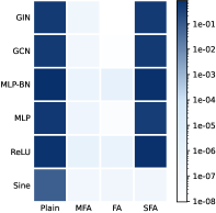
(a) $\mathrm{O}(3)$	(b) $\mathrm{O}(5)$
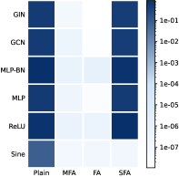
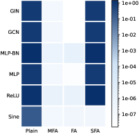
(c) $\mathrm{SO}(3)$	(d) $\mathrm{SO}(5)$
(e) $\mathrm{E}(3)$	(f) $\mathrm{E}(5)$
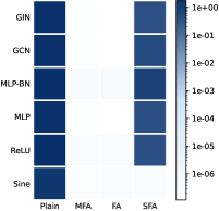
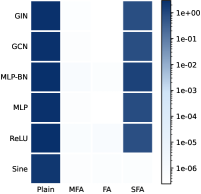
(g) $\mathrm{SE}(3)$	(h) $\mathrm{SE}(5)$

Figure 1: Comparative illustrations of equivariance test on the groups $\mathrm{O}(3),\mathrm{O}(5),\mathrm{SO}(3),\mathrm{SO}(5),\mathrm{E}(3),\mathrm{E}(5),\mathrm{SE}(3)$, and $\mathrm{SE}(5)$. Figures (a) and (b) depict the outcomes for $\mathrm{O}(3)$ and $\mathrm{O}(5)$, figures (c) and (d) display the results for $\mathrm{SO}(3)$ and $\mathrm{SO}(5)$, figures (e) and (f) show the results for $\mathrm{E}(3)$ and $\mathrm{E}(5)$, figures (g) and (h) demonstrate the results for $\mathrm{SE}(3)$ and $\mathrm{SE}(5)$, respectively. Data for left column is randomly sampled with a shape of $100\times 3$ and data for the right column is randomly sampled with a shape of $20\times 5$. All figures show the effectiveness of both our frame averaging method and original frame averaging method (Puny et al., 2021).

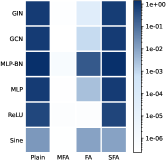
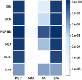
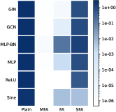
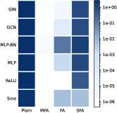
(a) $\mathrm{O}(5)$	(b) $\mathrm{SO}(5)$	(c) $\mathrm{E}(5)$	(d) $\mathrm{SE}(5)$

Figure 2: Illustrations of equivariance test on the groups $\mathrm{O}(5),\mathrm{SO}(5),\mathrm{E}(5),\mathrm{SE}(5)$ with degenerate singular values. All data is randomly sampled with a shape of $20\times 5$ with $3$ repeated singular values. As shown above, the original frame averaging method (Puny et al., 2021) fails the degenerate cases due to the repeated eigenvalues causing the frame size into infinity, while our method is not affected by the repeated eigenvalues and our minimal frame averaging is still equivariant to these groups.

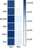
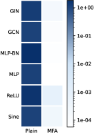
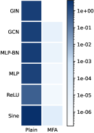
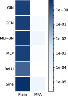
(a) $\mathrm{O}(1,3)$	(b) $\mathrm{SO}(1,3)$	(c) $\mathrm{GL}(3,\mathbb{R})$	(d) $\mathrm{SL}(3,\mathbb{R})$

Figure 3: Illustrations of equivariance test on the groups $\mathrm{O}(1,3),\mathrm{SO}(1,3),\mathrm{GL}(3,\mathbb{R}),\mathrm{SL}(3,\mathbb{R})$. As the original frame averaging method (Puny et al., 2021) does not give the frame construction for these groups, we only compare with the model without our method. The data for $\mathrm{O}(1,3)$ and $\mathrm{SO}(1,3)$ is randomly sampled with a shape of $100\times 4$, and data for $\mathrm{GL}(3,\mathbb{R})$ and $\mathrm{SL}(3,\mathbb{R})$ is randomly sampled with a shape of $100\times 3$. All the error scaling our method in the figures of is below $1e^{1e-3}$, showing that our method is indeed equivariant with respect to these group.

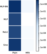
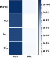
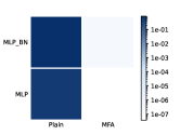
(a) $\mathrm{U}(3)$	(b) $\mathrm{SU}(3)$	(c) $\mathrm{S}_{n}\times\mathrm{O}(3)$	(d) $\mathrm{S}_{n}\times\mathrm{O}(1,3)$

Figure 4: Illustrations of equivariance test on the groups $\mathrm{U}(3),\mathrm{SU}(3),\mathrm{S}_{n},\mathrm{S}_{n}\times\mathrm{O}(3),\mathrm{S}_{n}\times\mathrm{O}(1,3)$. In (d), the first two rows correspond to the error test of $\mathrm{S}_{n}\times\mathrm{O}(3)$ and the last two rows correspond to that of $\mathrm{S}_{n}\times\mathrm{O}(1,3)$. As the original frame averaging method (Puny et al., 2021) does not give the frame construction for these groups, we only compare with the model without our method. The data for $\mathrm{U}(3)$ and $\mathrm{SU}(3)$ is randomly sampled with a shape of $100\times 3$, data for $\mathrm{S}_{n}\times\mathrm{O}(3)$ is randomly sampled with a shape of $32\times 3$, and data for $\mathrm{S}_{n}\times\mathrm{O}(1,3)$ is randomly sampled with a shape of $32\times 4$. Note that the networks used for these groups are different from the previous groups to accommodate the properties of these groups. The MLP models used for both $\mathrm{U}(3)$ and $\mathrm{SU}(3)$ are complex valued networks, and the MLP models used for $\mathrm{S}_{n}\times\mathrm{O}(3)$ and $\mathrm{S}_{n}\times\mathrm{O}(1,3)$ are transforming both the node dimension and the feature dimension, and are neither $\mathrm{S}_{n}\times\mathrm{O}(3)$ nor $\mathrm{S}_{n}\times\mathrm{O}(1,3)$-equivariant. Specially, the $\mathrm{S}_{n}\times\mathrm{O}(3)$ or $\mathrm{S}_{n}\times\mathrm{O}(1,3)$-equivariant frame is created by applying $\mathrm{S}_{n}$-equivariant and $\mathrm{O}(3)$ or $\mathrm{O}(1,3)$-invariant frame to the MLP with $\mathrm{O}(3)$ or $\mathrm{O}(1,3)$-equivariant frame, corresponding to Section 5.3.

I.2 $n$-Body Problem

Model.

Similar to Puny et al. (2021); Kaba et al. (2023); Ruhe et al. (2023), our model follows the architecture proposed by Satorras et al. (2021). Inspired by Ruhe et al. (2023), it integrates layer normalization (Ba et al., 2016) and dropout (Hinton et al., 2012) in message passing layers. The architecture consists of 4 message passing layers, each with a hidden dimension of 60, and employs a dropout rate of 0.1. Our generalized QR decomposition is used to compute the $\mathrm{O}(3)$-equivariant frame, which maintains a constant size of 1 across all data points, ensuring model equivariance with a single forward pass.

Training.

The model is optimized using a Mean Absolute Error (MAE) loss criterion, employing the Adam optimizer (Kingma & Ba, 2014). Training parameters include a batch size of 100, a learning rate of $1\times 10^{-3}$, and a weight decay of $5\times 10^{-6}$ over 10,000 epochs. During training, to alleviate the discontinuity of canonicalization, input augmentation through random rotations is applied, and FA-GNN is retrained under identical settings for fair comparison. Training and evaluation are conducted on a single NVIDIA GeForce RTX 2080 Ti GPU.

I.3 Open Catalyst Dataset

Model.

We perform a direct comparison to FAENet by training it using the MFA paradigm with generalized QR decomposition in place of stochastic frame averaging as used by Duval et al. (2023b). Network configurations include a radius cutoff of 6.0, 5 interaction layers, and a hidden dimension of 384. Frames are calculated based on an identical point projection to 2D as employed by Duval et al. (2023b).

Training.

The Adam optimizer is employed with a batch size of 256 and an initial learning rate of $2\times 10^{-3}$, adjusted by a cosine annealing scheduler over 12 epochs. Random reflection augmentation is used during training. The model is trained and evaluated on an NVIDIA A100 GPU. Comprehensive results for the OC20 dataset are presented in Table 9.

Table 9: Results on the IS2RE (initial structure to relaxed energy) task from OC20 (Chanussot et al., 2021). Models are trained and evaluated on the IS2RE direct task, where the relaxed energy is predicted directly from the initial structure, as opposed to via relaxation or Noisy Nodes data augmentation (Godwin et al., 2022; Liao & Smidt, 2022). Baselines are SchNet (Schütt et al., 2018), DimeNet++ (Gasteiger et al., 2020), GemNet-T (Gasteiger et al., 2019), SphereNet (Liu et al., 2022), ComENet (Wang et al., 2022a), SEGNN (Brandstetter et al., 2021), Equiformer (Liao & Smidt, 2022) and FAENet (Duval et al., 2023b).

	Energy MAE [eV]					EwT
Model	ID	OOD-Cat	OOD-Ads	OOD-Both	Average	ID	OOD-Cat	OOD-Ads	OOD-Both	Average
SchNet	0.6372	0.6611	0.7342	0.7035	0.6840	2.96%	3.03%	2.22%	2.38%	2.65%
DimeNet++	0.5716	0.5612	0.7224	0.6615	0.6283	4.26%	4.10%	2.06%	3.21%	3.40%
GemNet-T	0.5561	0.5659	0.7342	0.6964	0.6382	4.51%	4.37%	2.24%	2.38%	3.38%
SphereNet	0.5632	0.5590	0.6682	0.6190	0.6024	4.56 %	4.59 %	2.70 %	2.70 %	3.64%
ComENet	0.5558	0.5491	0.6602	0.5901	0.5888	4.17%	4.53%	2.71%	2.83%	3.56%
SEGNN	0.5310	0.5341	0.6432	0.5777	0.5715	5.32%	4.89 %	2.80 %	3.09 %	4.03 %
Equiformer	0.5088	0.5051	0.6271	0.5545	0.5489	4.88 %	4.92 %	2.93 %	2.98 %	3.93 %
FAENet	0.5446	0.5707	0.6115	0.5449	0.5679	4.46%	4.67%	2.95 %	3.01 %	3.78%
MFAENet	0.5437	0.5415	0.6203	0.5708	0.5691	4.33%	4.54%	2.96 %	2.97 %	3.70%

I.4 Top Tagging Dataset

Model.

LorentzNet (Gong et al., 2022) is an very strong $\mathrm{O}(1,3)$-invariant baseline developed specifically for the top tagging task. Each layer of LorentzNet is designed to be $\mathrm{O}(1,3)$-equivariant and the final output is $\mathrm{O}(1,3)$-invariant. We replace the invariant layer with the outer product between the invariant features and equivariant vectors, following batch normalization and nonlinearities, thereby breaking the invariance of the final output. The model, termed MinkGNN, incorporates 6 message passing layers with a hidden dimension of 72. Further refinement is achieved through our generalized QR decomposition to establish an $\mathrm{O}(1,3)$-invariant frame, resulting in an $\mathrm{O}(1,3)$-invariant model referred to as MFA-MinkGNN.

Training.

Both MinkGNN and MFA-MinkGNN are optimized using the Adam optimizer, with a batch size of 64, a learning rate of $5\times 10^{-4}$, a weight decay of $1\times 10^{-2}$, and a cosine annealing scheduler over 100 epochs. We then evaluate them with the Exponential Moving Average (EMA) with a decay of 0.995. Training and evaluation are conducted on 1 NVIDIA A100 GPU. Comprehensive results for the top tagging dataset are presented in Table 10.

Table 10: Accuracy and AUC for the top tagging experiment. Baselines are ResNeXt (Xie et al., 2017), ParticleNet (Qu & Gouskos, 2020), EGNN (Satorras et al., 2021), LGN (Bogatskiy et al., 2020), LorentzNet (Gong et al., 2022), and CGENN (Ruhe et al., 2023).

Method	Accuracy	AUC
ResNeXt	0.936	0.9837
ParticleNet	0.940	0.9858
EGNN	0.922	0.9760
LGN	0.929	0.9640
LorentzNet	0.942	0.9868
CGENN	0.942	0.9869
MFA-MinkGNN	0.942	0.9869

I.5 Graph Separation

Model.

For both the Graph8c and EXP datasets, we adopt the MLP and GIN models as used by Puny et al. (2021) for the graph separation task. Using our custom implementation of the nauty canonical labeling algorithm (McKay, 2007), we generate canonical graphs for each sample and concatenate these to their respective inputs. Given the directed graph input and the permutation invariance of the task, frame sampling is unnecessary, allowing direct computation as per Equation 4.

Training.

Optimization is performed using the Adam optimizer, with settings including a learning rate of 0.001 and a batch size of 100 across 200 epochs.

I.6 Convex Hull

Model.

We employ a MLP model with a hidden dimension of 32 for projections of both the feature and node dimensions, rendering the model neither $\mathrm{S}_{n}$-invariant nor $\mathrm{O}(5)$-invariant. After being centered, vectors from the origin of points are used as input. The frame is made $\mathrm{S}_{n}$-equivariant and $\mathrm{O}(5)$-invariant using the inner product matrix of vectors and is subsequently applied to a $\mathrm{O}(5)$-invariant frame to achieve an $\mathrm{S}_{n}\times\mathrm{O}(5)$-invariant frame averaging. The canonicalization of the inner product matrix follows the methodology described in Appendix F.

Training.

The convex hull dataset, comprising 16,384 samples for each of the training, validation, and test sets, is generated following Ruhe et al. (2023). Training utilizes the Adam optimizer with a learning rate of 0.001, a batch size of 128, and a cosine annealing scheduler.

References

- ATL (2022) Constituent-Based Top-Quark Tagging with the ATLAS Detector. Technical report, CERN, Geneva, 2022. URL https://cds.cern.ch/record/2825328.
- Anderson et al. (2019) Anderson, B., Hy, T. S., and Kondor, R. Cormorant: Covariant molecular neural networks. Advances in neural information processing systems, 32, 2019.
- Atzmon et al. (2022) Atzmon, M., Nagano, K., Fidler, S., Khamis, S., and Lipman, Y. Frame averaging for equivariant shape space learning. In Proceedings of the IEEE/CVF Conference on Computer Vision and Pattern Recognition, pp. 631–641, 2022.
- Ba et al. (2016) Ba, J. L., Kiros, J. R., and Hinton, G. E. Layer normalization. arXiv preprint arXiv:1607.06450, 2016.
- Batatia et al. (2022) Batatia, I., Kovacs, D. P., Simm, G. N., Ortner, C., and Csanyi, G. Mace: Higher order equivariant message passing neural networks for fast and accurate force fields. In Advances in Neural Information Processing Systems, 2022.
- Batzner et al. (2022) Batzner, S., Musaelian, A., Sun, L., Geiger, M., Mailoa, J. P., Kornbluth, M., Molinari, N., Smidt, T. E., and Kozinsky, B. E (3)-equivariant graph neural networks for data-efficient and accurate interatomic potentials. Nature communications, 13(1):2453, 2022.
- Bogatskiy et al. (2020) Bogatskiy, A., Anderson, B., Offermann, J., Roussi, M., Miller, D., and Kondor, R. Lorentz group equivariant neural network for particle physics. In International Conference on Machine Learning, pp. 992–1002. PMLR, 2020.
- Brandstetter et al. (2021) Brandstetter, J., Hesselink, R., van der Pol, E., Bekkers, E. J., and Welling, M. Geometric and physical quantities improve e (3) equivariant message passing. In International Conference on Learning Representations, 2021.
- Bronstein et al. (2021) Bronstein, M. M., Bruna, J., Cohen, T., and Veličković, P. Geometric deep learning: Grids, groups, graphs, geodesics, and gauges. arXiv preprint arXiv:2104.13478, 2021.
- Chanussot et al. (2021) Chanussot, L., Das, A., Goyal, S., Lavril, T., Shuaibi, M., Riviere, M., Tran, K., Heras-Domingo, J., Ho, C., Hu, W., Palizhati, A., Sriram, A., Wood, B., Yoon, J., Parikh, D., Zitnick, C. L., and Ulissi, Z. Open catalyst 2020 (oc20) dataset and community challenges. ACS Catalysis, 2021. doi: 10.1021/acscatal.0c04525.
- Chen et al. (2022) Chen, H., Hendry, D. G., Weinberg, P. E., and Feiguin, A. Systematic improvement of neural network quantum states using lanczos. In Oh, A. H., Agarwal, A., Belgrave, D., and Cho, K. (eds.), Advances in Neural Information Processing Systems, 2022. URL https://openreview.net/forum?id=qZUHvvtbzy.
- Cohen & Welling (2016a) Cohen, T. and Welling, M. Group equivariant convolutional networks. In International conference on machine learning, pp. 2990–2999. PMLR, 2016a.
- Cohen & Welling (2016b) Cohen, T. S. and Welling, M. Steerable cnns. In International Conference on Learning Representations, 2016b.
- Du et al. (2022) Du, W., Zhang, H., Du, Y., Meng, Q., Chen, W., Zheng, N., Shao, B., and Liu, T.-Y. Se (3) equivariant graph neural networks with complete local frames. In International Conference on Machine Learning, pp. 5583–5608. PMLR, 2022.
- Duval et al. (2023a) Duval, A., Mathis, S. V., Joshi, C. K., Schmidt, V., Miret, S., Malliaros, F. D., Cohen, T., Liò, P., Bengio, Y., and Bronstein, M. A hitchhiker’s guide to geometric gnns for 3d atomic systems. arXiv preprint arXiv:2312.07511, 2023a.
- Duval et al. (2023b) Duval, A. A., Schmidt, V., Hernandez-Garcia, A., Miret, S., Malliaros, F. D., Bengio, Y., and Rolnick, D. Faenet: Frame averaging equivariant gnn for materials modeling. In International Conference on Machine Learning, pp. 9013–9033. PMLR, 2023b.
- Dym & Gortler (2024) Dym, N. and Gortler, S. J. Low-dimensional invariant embeddings for universal geometric learning. Foundations of Computational Mathematics, pp. 1–41, 2024.
- Dym et al. (2024) Dym, N., Lawrence, H., and Siegel, J. W. Equivariant frames and the impossibility of continuous canonicalization. arXiv preprint arXiv:2402.16077, 2024.
- Esteves et al. (2020) Esteves, C., Makadia, A., and Daniilidis, K. Spin-weighted spherical cnns. Advances in Neural Information Processing Systems, 33:8614–8625, 2020.
- Fu et al. (2023) Fu, C., Yan, K., Wang, L., Au, W. Y., McThrow, M., Komikado, T., Maruhashi, K., Uchino, K., Qian, X., and Ji, S. A latent diffusion model for protein structure generation. In The Second Learning on Graphs Conference, 2023.
- Fuchs et al. (2020) Fuchs, F., Worrall, D., Fischer, V., and Welling, M. Se (3)-transformers: 3d roto-translation equivariant attention networks. Advances in neural information processing systems, 33:1970–1981, 2020.
- Gasteiger et al. (2019) Gasteiger, J., Groß, J., and Günnemann, S. Directional message passing for molecular graphs. In International Conference on Learning Representations, 2019.
- Gasteiger et al. (2020) Gasteiger, J., Giri, S., Margraf, J. T., and Günnemann, S. Fast and uncertainty-aware directional message passing for non-equilibrium molecules. arXiv preprint arXiv:2011.14115, 2020.
- Gasteiger et al. (2021) Gasteiger, J., Becker, F., and Günnemann, S. Gemnet: Universal directional graph neural networks for molecules. Advances in Neural Information Processing Systems, 34:6790–6802, 2021.
- Godwin et al. (2022) Godwin, J., Schaarschmidt, M., Gaunt, A. L., Sanchez-Gonzalez, A., Rubanova, Y., Veličković, P., Kirkpatrick, J., and Battaglia, P. Simple GNN regularisation for 3d molecular property prediction and beyond. In International Conference on Learning Representations, 2022. URL https://openreview.net/forum?id=1wVvweK3oIb.
- Gong et al. (2022) Gong, S., Meng, Q., Zhang, J., Qu, H., Li, C., Qian, S., Du, W., Ma, Z.-M., and Liu, T.-Y. An efficient lorentz equivariant graph neural network for jet tagging. Journal of High Energy Physics, 2022(7):1–22, 2022.
- Gui et al. (2022) Gui, S., Li, X., Wang, L., and Ji, S. Good: A graph out-of-distribution benchmark. Advances in Neural Information Processing Systems, 35:2059–2073, 2022.
- Gui et al. (2024) Gui, S., Liu, M., Li, X., Luo, Y., and Ji, S. Joint learning of label and environment causal independence for graph out-of-distribution generalization. Advances in Neural Information Processing Systems, 36, 2024.
- Han et al. (2022) Han, J., Rong, Y., Xu, T., and Huang, W. Geometrically equivariant graph neural networks: A survey. arXiv preprint arXiv:2202.07230, 2022.
- Helwig et al. (2023) Helwig, J., Zhang, X., Fu, C., Kurtin, J., Wojtowytsch, S., and Ji, S. Group equivariant Fourier neural operators for partial differential equations. In Proceedings of the 40th International Conference on Machine Learning, 2023.
- Hinton et al. (2012) Hinton, G. E., Srivastava, N., Krizhevsky, A., Sutskever, I., and Salakhutdinov, R. R. Improving neural networks by preventing co-adaptation of feature detectors. arXiv preprint arXiv:1207.0580, 2012.
- Hoogeboom et al. (2022) Hoogeboom, E., Satorras, V. G., Vignac, C., and Welling, M. Equivariant diffusion for molecule generation in 3d. In International conference on machine learning, pp. 8867–8887. PMLR, 2022.
- Horie et al. (2021) Horie, M., Morita, N., Hishinuma, T., Ihara, Y., and Mitsume, N. Isometric transformation invariant and equivariant graph convolutional networks. In International Conference on Learning Representations, 2021. URL https://openreview.net/forum?id=FX0vR39SJ5q.
- Horn & Johnson (2012) Horn, R. A. and Johnson, C. R. Matrix analysis. Cambridge university press, 2012.
- Huang et al. (2022) Huang, W., Han, J., Rong, Y., Xu, T., Sun, F., and Huang, J. Equivariant graph mechanics networks with constraints. In International Conference on Learning Representations, 2022. URL https://openreview.net/forum?id=SHbhHHfePhP.
- Jing et al. (2021) Jing, B., Eismann, S., Suriana, P., Townshend, R. J. L., and Dror, R. Learning from protein structure with geometric vector perceptrons. In International Conference on Learning Representations, 2021. URL https://openreview.net/forum?id=1YLJDvSx6J4.
- Kaba et al. (2023) Kaba, S.-O., Mondal, A. K., Zhang, Y., Bengio, Y., and Ravanbakhsh, S. Equivariance with learned canonicalization functions. In International Conference on Machine Learning, pp. 15546–15566. PMLR, 2023.
- Kasieczka et al. (2019a) Kasieczka, G., Plehn, T., Butter, A., Cranmer, K., Debnath, D., Dillon, B. M., Fairbairn, M., Faroughy, D. A., Fedorko, W., Gay, C., et al. The machine learning landscape of top taggers. SciPost Physics, 7(1):014, 2019a.
- Kasieczka et al. (2019b) Kasieczka, G., Plehn, T., Thompson, J., and Russel, M. Top quark tagging reference dataset, March 2019b. URL https://doi.org/10.5281/zenodo.2603256.
- Kiani et al. (2024) Kiani, B. T., Le, T., Lawrence, H., Jegelka, S., and Weber, M. On the hardness of learning under symmetries. arXiv preprint arXiv:2401.01869, 2024.
- Kim et al. (2023) Kim, J., Nguyen, D. T., Suleymanzade, A., An, H., and Hong, S. Learning probabilistic symmetrization for architecture agnostic equivariance. In Thirty-seventh Conference on Neural Information Processing Systems, 2023. URL https://openreview.net/forum?id=phnN1eu5AX.
- Kingma & Ba (2014) Kingma, D. P. and Ba, J. Adam: A method for stochastic optimization. arXiv preprint arXiv:1412.6980, 2014.
- Kipf et al. (2018) Kipf, T., Fetaya, E., Wang, K.-C., Welling, M., and Zemel, R. Neural relational inference for interacting systems. In International conference on machine learning, pp. 2688–2697. PMLR, 2018.
- Kipf & Welling (2016) Kipf, T. N. and Welling, M. Semi-supervised classification with graph convolutional networks. arXiv preprint arXiv:1609.02907, 2016.
- Köhler et al. (2020) Köhler, J., Klein, L., and Noé, F. Equivariant flows: exact likelihood generative learning for symmetric densities. In International conference on machine learning, pp. 5361–5370. PMLR, 2020.
- Kondor & Trivedi (2018) Kondor, R. and Trivedi, S. On the generalization of equivariance and convolution in neural networks to the action of compact groups. In International conference on machine learning, pp. 2747–2755. PMLR, 2018.
- Lawrence & Harris (2023) Lawrence, H. and Harris, M. T. Learning polynomial problems with sl (2)-equivariance. 2023.
- Li et al. (2023) Li, X., Gui, S., Luo, Y., and Ji, S. Graph structure and feature extrapolation for out-of-distribution generalization. arXiv preprint arXiv:2306.08076, 2023.
- Liao & Smidt (2022) Liao, Y.-L. and Smidt, T. Equiformer: Equivariant graph attention transformer for 3d atomistic graphs. In The Eleventh International Conference on Learning Representations, 2022.
- Lim et al. (2024) Lim, D., Robinson, J., Jegelka, S., and Maron, H. Expressive sign equivariant networks for spectral geometric learning. Advances in Neural Information Processing Systems, 36, 2024.
- Lin et al. (2023) Lin, Y., Yan, K., Luo, Y., Liu, Y., Qian, X., and Ji, S. Efficient approximations of complete interatomic potentials for crystal property prediction. 2023. URL https://openreview.net/forum?id=KaKXygtEGK.
- Liu et al. (2022) Liu, Y., Wang, L., Liu, M., Lin, Y., Zhang, X., Oztekin, B., and Ji, S. Spherical message passing for 3d molecular graphs. In International Conference on Learning Representations, 2022. URL https://openreview.net/forum?id=givsRXsOt9r.
- Luo et al. (2023) Luo, Y., Liu, C., and Ji, S. Towards symmetry-aware generation of periodic materials. In Thirty-seventh Conference on Neural Information Processing Systems, 2023.
- Ma et al. (2024) Ma, G., Wang, Y., and Wang, Y. Laplacian canonization: A minimalist approach to sign and basis invariant spectral embedding. Advances in Neural Information Processing Systems, 36, 2024.
- McKay (2007) McKay, B. D. Nauty user’s guide (version 2.4). Computer Science Dept., Australian National University, pp. 225–239, 2007.
- McKay & Piperno (2014) McKay, B. D. and Piperno, A. Practical graph isomorphism, ii. Journal of symbolic computation, 60:94–112, 2014.
- Mondal et al. (2024) Mondal, A. K., Panigrahi, S. S., Kaba, O., Mudumba, S. R., and Ravanbakhsh, S. Equivariant adaptation of large pretrained models. Advances in Neural Information Processing Systems, 36, 2024.
- Nguyen et al. (2023) Nguyen, T. D., Kim, J., Yang, H., and Hong, S. Learning symmetrization for equivariance with orbit distance minimization. arXiv preprint arXiv:2311.07143, 2023.
- Pozdnyakov & Ceriotti (2024) Pozdnyakov, S. and Ceriotti, M. Smooth, exact rotational symmetrization for deep learning on point clouds. Advances in Neural Information Processing Systems, 36, 2024.
- Puny et al. (2021) Puny, O., Atzmon, M., Ben-Hamu, H., Misra, I., Grover, A., Smith, E. J., and Lipman, Y. Frame averaging for invariant and equivariant network design. arXiv preprint arXiv:2110.03336, 2021.
- Puny et al. (2023) Puny, O., Lim, D., Kiani, B., Maron, H., and Lipman, Y. Equivariant polynomials for graph neural networks. In International Conference on Machine Learning, pp. 28191–28222. PMLR, 2023.
- Qi et al. (2017) Qi, C. R., Su, H., Mo, K., and Guibas, L. J. Pointnet: Deep learning on point sets for 3d classification and segmentation. In Proceedings of the IEEE conference on computer vision and pattern recognition, pp. 652–660, 2017.
- Qu & Gouskos (2020) Qu, H. and Gouskos, L. Jet tagging via particle clouds. Physical Review D, 101(5):056019, 2020.
- Ruhe et al. (2023) Ruhe, D., Brandstetter, J., and Forré, P. Clifford group equivariant neural networks. In Thirty-seventh Conference on Neural Information Processing Systems, 2023. URL https://openreview.net/forum?id=n84bzMrGUD.
- Satorras et al. (2021) Satorras, V. G., Hoogeboom, E., and Welling, M. E(n) equivariant graph neural networks. In International conference on machine learning, pp. 9323–9332. PMLR, 2021.
- Schütt et al. (2021) Schütt, K., Unke, O., and Gastegger, M. Equivariant message passing for the prediction of tensorial properties and molecular spectra. In International Conference on Machine Learning, pp. 9377–9388. PMLR, 2021.
- Schütt et al. (2018) Schütt, K. T., Sauceda, H. E., Kindermans, P.-J., Tkatchenko, A., and Müller, K.-R. Schnet–a deep learning architecture for molecules and materials. The Journal of Chemical Physics, 148(24), 2018.
- Smidt et al. (2021) Smidt, T. E., Geiger, M., and Miller, B. K. Finding symmetry breaking order parameters with euclidean neural networks. Physical Review Research, 3(1):L012002, 2021.
- Stärk et al. (2022) Stärk, H., Ganea, O., Pattanaik, L., Barzilay, R., and Jaakkola, T. Equibind: Geometric deep learning for drug binding structure prediction. In International conference on machine learning, pp. 20503–20521. PMLR, 2022.
- Tauvel & Yu (2005) Tauvel, P. and Yu, R. W. Homogeneous spaces and quotients. Lie Algebras and Algebraic Groups, pp. 387–399, 2005.
- Thölke & De Fabritiis (2021) Thölke, P. and De Fabritiis, G. Equivariant transformers for neural network based molecular potentials. In International Conference on Learning Representations, 2021.
- Thomas et al. (2018) Thomas, N., Smidt, T., Kearnes, S., Yang, L., Li, L., Kohlhoff, K., and Riley, P. Tensor field networks: Rotation-and translation-equivariant neural networks for 3d point clouds. arXiv preprint arXiv:1802.08219, 2018.
- Unke et al. (2021) Unke, O., Bogojeski, M., Gastegger, M., Geiger, M., Smidt, T., and Müller, K.-R. Se (3)-equivariant prediction of molecular wavefunctions and electronic densities. Advances in Neural Information Processing Systems, 34:14434–14447, 2021.
- Villar et al. (2021) Villar, S., Hogg, D. W., Storey-Fisher, K., Yao, W., and Blum-Smith, B. Scalars are universal: Equivariant machine learning, structured like classical physics. In Beygelzimer, A., Dauphin, Y., Liang, P., and Vaughan, J. W. (eds.), Advances in Neural Information Processing Systems, 2021. URL https://openreview.net/forum?id=ba27-RzNaIv.
- Wang et al. (2022a) Wang, L., Liu, Y., Lin, Y., Liu, H., and Ji, S. ComENet: Towards complete and efficient message passing for 3d molecular graphs. In Oh, A. H., Agarwal, A., Belgrave, D., and Cho, K. (eds.), Advances in Neural Information Processing Systems, 2022a. URL https://openreview.net/forum?id=mCzMqeWSFJ.
- Wang et al. (2023a) Wang, L., Liu, H., Liu, Y., Kurtin, J., and Ji, S. Learning hierarchical protein representations via complete 3d graph networks. In International Conference on Learning Representations (ICLR), 2023a.
- Wang et al. (2020) Wang, R., Walters, R., and Yu, R. Incorporating symmetry into deep dynamics models for improved generalization. In International Conference on Learning Representations, 2020.
- Wang et al. (2022b) Wang, R., Walters, R., and Yu, R. Approximately equivariant networks for imperfectly symmetric dynamics. In International Conference on Machine Learning, pp. 23078–23091. PMLR, 2022b.
- Wang et al. (2023b) Wang, R., Walters, R., and Smidt, T. Relaxed octahedral group convolution for learning symmetry breaking in 3d physical systems. In NeurIPS 2023 AI for Science Workshop, 2023b.
- Weiler et al. (2018) Weiler, M., Geiger, M., Welling, M., Boomsma, W., and Cohen, T. S. 3d steerable cnns: Learning rotationally equivariant features in volumetric data. Advances in Neural Information Processing Systems, 31, 2018.
- Worrall & Welling (2019) Worrall, D. and Welling, M. Deep scale-spaces: Equivariance over scale. Advances in Neural Information Processing Systems, 32, 2019.
- Xie et al. (2017) Xie, S., Girshick, R., Dollár, P., Tu, Z., and He, K. Aggregated residual transformations for deep neural networks. In Proceedings of the IEEE conference on computer vision and pattern recognition, pp. 1492–1500, 2017.
- Xu et al. (2018) Xu, K., Hu, W., Leskovec, J., and Jegelka, S. How powerful are graph neural networks? arXiv preprint arXiv:1810.00826, 2018.
- Xu et al. (2023) Xu, M., Powers, A. S., Dror, R. O., Ermon, S., and Leskovec, J. Geometric latent diffusion models for 3d molecule generation. In International Conference on Machine Learning, pp. 38592–38610. PMLR, 2023.
- Xu et al. (2021) Xu, Z., Luo, Y., Zhang, X., Xu, X., Xie, Y., Liu, M., Dickerson, K., Deng, C., Nakata, M., and Ji, S. Molecule3d: A benchmark for predicting 3d geometries from molecular graphs. arXiv preprint arXiv:2110.01717, 2021.
- Yan et al. (2022) Yan, K., Liu, Y., Lin, Y., and Ji, S. Periodic graph transformers for crystal material property prediction. Advances in Neural Information Processing Systems, 35:15066–15080, 2022.
- Yan et al. (2024) Yan, K., Fu, C., Qian, X., Qian, X., and Ji, S. Complete and efficient graph transformers for crystal material property prediction. arXiv preprint arXiv:2403.11857, 2024.
- Yarotsky (2022) Yarotsky, D. Universal approximations of invariant maps by neural networks. Constructive Approximation, 55(1):407–474, 2022.
- Yu et al. (2023) Yu, H., Xu, Z., Qian, X., Qian, X., and Ji, S. Efficient and equivariant graph networks for predicting quantum hamiltonian. In International Conference on Machine Learning. PMLR, 2023.
- Zhang et al. (2023) Zhang, X., Wang, L., Helwig, J., Luo, Y., Fu, C., Xie, Y., Liu, M., Lin, Y., Xu, Z., Yan, K., et al. Artificial intelligence for science in quantum, atomistic, and continuum systems. arXiv preprint arXiv:2307.08423, 2023.