Rate-Preserving Reductions for Blackwell Approachability

Abstract

Abernethy et al. (2011) showed that Blackwell approachability and no-regret learning are equivalent, in the sense that any algorithm that solves a specific Blackwell approachability instance can be converted to a sublinear regret algorithm for a specific no-regret learning instance, and vice versa. In this paper, we study a more fine-grained form of such reductions, and ask when this translation between problems preserves not only a sublinear rate of convergence, but also preserves the optimal rate of convergence. That is, in which cases does it suffice to find the optimal regret bound for a no-regret learning instance in order to find the optimal rate of convergence for a corresponding approachability instance?

We show that the reduction of Abernethy et al. (2011) does not preserve rates: their reduction may reduce a $d$-dimensional approachability instance $\mathcal{I}_{1}$ with optimal convergence rate $R_{1}$ to a no-regret learning instance $\mathcal{I}_{2}$ with optimal regret-per-round of $R_{2}$, with $R_{2}/R_{1}$ arbitrarily large (in particular, it is possible that $R_{1}=0$ and $R_{2}>0$). On the other hand, we show that it is possible to tightly reduce any approachability instance to an instance of a generalized form of regret minimization we call improper $\phi$-regret minimization (a variant of the $\phi$-regret minimization of Gordon et al. (2008) where the transformation functions may map actions outside of the action set).

Finally, we characterize when linear transformations suffice to reduce improper $\phi$-regret minimization problems to standard classes of regret minimization problems (such as external regret minimization and proper $\phi$-regret minimization) in a rate preserving manner. We prove that some improper $\phi$-regret minimization instances cannot be reduced to either subclass of instance in this way, suggesting that approachability can capture some problems that cannot be easily phrased in the standard language of online learning.

1 Introduction

Blackwell’s Approachability Theorem is a fundamental result in game theory with far-reaching applications in machine learning, economics, and optimization. It provides a framework for analyzing repeated games where the payoff is a vector rather than a single scalar value. In essence, the theorem allows players to determine whether a specific set of payoff vectors can be “approached” on average over time, even if achieving them individually in a single round is impossible (with more sophisticated variants of this theorem characterizing the rate at which this set can be approached). This concept has been instrumental in developing robust algorithms for online learning, strategic decision-making in economic models, and solving complex optimization problems where the objective is multi-dimensional.

A perhaps even more prevalent paradigm in the area of online learning is that of regret minimization. In the most fundamental form of the problem (external regret minimization), a learner wants to take a sequence of actions that performs at least as well as the optimal static action they could have taken in hindsight. One of the central results of the field of online learning is that there exist learning algorithms which achieve regret that is sublinear in the time horizon $T$. Understanding how to optimize these regret bounds is a topic of active research, and optimal regret bounds have been established for a variety of problems in this area.

Abernethy et al. (2011) showed that these two problems – Blackwell approachability and regret minimization – are very closely linked, and in fact are “equivalent” in the following sense: given an instance of Blackwell approachability (a vector-valued payoff function and a set to approach), it is possible to reduce it to an instance of regret minimization (specifically, an instance of online linear optimization) such that any sublinear regret algorithm for the regret minimization instance can be used to solve the corresponding Blackwell approachability instance, giving an algorithmic proof of convergence. Conversely, any regret minimization instance can itself be viewed as an instance of Blackwell approachability, so any algorithmic approach to generic Blackwell approachability instances can be applied to solve regret minimization.

In this paper, we explore whether such an equivalence holds at a more fine-grained level, when we care about the specific convergence rates for Blackwell approachability and the specific regret bounds for regret minimization. In other words, imagine we have a problem that we can cast as a specific instance of Blackwell approachability, and we want to understand the optimal convergence rates possible for this instance (this is a common desideratum for many of the aforementioned applications of approachability). Is it sufficient to just understand the optimal regret bounds for the corresponding instance of regret minimization under the reduction of Abernethy et al. (2011)?

1.1 Our results

We begin by answering this question in the negative: there is no direct correspondence between the optimal rate achievable in an approachability instance $\mathcal{I}$ and the optimal regret bound achievable in the corresponding regret minimization instance $\mathcal{I}^{\prime}$. More precisely, the algorithmic construction of Abernethy et al. (2011) shows that any upper bound on the regret of $\mathcal{I}’$ translates to an upper bound on the optimal convergence rate of $\mathcal{I}$. We prove that this translation is lossy, and that there is no analogous translation between lower bounds. In particular, in Theorem 3 we exhibit instances of approachability $\mathcal{I}$ that are perfectly approachable (i.e., where the learner can guarantee that the average payoff exactly lies within the set $S$) but where the corresponding regret-minimization instance $\mathcal{I}^{\prime}$ has a non-trivial regret lower bound.

On the other hand, we complement this result by showing that Blackwell approachability can be tightly reduced (in a rate-preserving manner) to a novel variant of regret minimization that we call improper $\phi$-regret minimization (Theorem 4). To explain what this means, it is helpful to briefly define regret minimization and its relevant variants (we defer formal definitions to Section 2).

We start with the basic setting of online linear optimization. In this problem, a learner must select an action $p_{t}$ from a convex action set $\mathcal{P}\subseteq\mathbb{R}^{d}$ each round $t$ for a total of $T$ rounds. At the same time, an adversary selects a loss $\ell_{t}$ from a convex loss set $\mathcal{L}\subseteq\mathbb{R}^{d}$. The learner receives loss $\langle p_{t},\ell_{t}\rangle$ during that round, and would like to minimize their total regret over all rounds. In its most standard form (external regret), this is just the largest gap between their total loss and the total loss of the best fixed action, and can be written as

$$\operatorname{\mathsf{Reg}}({\mathbf{p}},{\bm{\ell}})=\max_{p^{*}\in\mathcal{P}}\left(\sum_{t=1}^{T}\langle p_{t},\ell_{t}\rangle-\sum_{t=1}^{T}\langle p^{*},\ell_{t}\rangle\right).$$

Some applications call for obtaining low regret not just with respect to the best fixed action in hindsight, but additionally with respect to transformations of the sequence of actions played by the learner. The most well-known such notion of regret is probably that of swap regret, which famously has the property that sublinear swap regret learning algorithms converge to correlated equilibria when used to play normal-form games (Foster and Vohra, 1997). However, swap regret is just one of a large class of such regret metrics that are succinctly captured by the notion of (linear) $\phi$-regret introduced in (Gordon et al., 2008). In $\phi$-regret minimization, we are given a collection $\Phi$ of linear “transformation” functions $\phi$ sending $\mathcal{P}$ to $\mathcal{P}$. The $\phi$-regret for this class $\Phi$ is given by:

$$\operatorname{\mathsf{Reg}}_{\Phi}({\mathbf{p}},{\bm{\ell}})=\max_{\phi\in\Phi}\left(\sum_{t=1}^{T}\langle p_{t},\ell_{t}\rangle-\sum_{t=1}^{T}\langle\phi(p_{t}),\ell_{t}\rangle\right).$$

Note that by setting $\Phi$ to be the set of all constant functions on $\mathcal{P}$, we immediately recover the original external regret definition. The case of swap regret corresponds to the setting where $\mathcal{P}$ is the $d$-simplex, and $\Phi$ contains all row-stochastic linear maps. Interestingly, in (Gordon et al., 2008), the authors show that any $\phi$-regret minimization problem has a corresponding sublinear regret learning algorithm (this can also be seen from Blackwell approachability).

However, the constraint that every linear function $\phi$ in $\Phi$ maps $\mathcal{P}$ to itself turns out not to be strictly necessary – there exist classes $\Phi$ of linear functions that map points in $\mathcal{P}$ to arbitrary points in $\mathbb{R}^{d}$ (including possibly outside of $\mathcal{P}$) for which it is still possible to obtain sublinear $\phi$-regret. We call any such instance an improper $\phi$-regret minimization instance (and contrast it with the previous constrained definition by calling those instances proper $\phi$-regret minimization). In Theorem 4, we show that for any Blackwell approachability instance $\mathcal{I}$, there exists an improper $\phi$-regret minimization instance $\mathcal{I}^{\prime}$, such that if you have an algorithm that solves $\mathcal{I}^{\prime}$ with at most $R$ $\phi$-regret, you can use it to get a convergence rate of $R/T$ in the approachability instance $\mathcal{I}$, and vice versa.

The introduction of improper $\phi$-regret raises a natural question: is improper $\phi$-regret minimization truly a more general setting than proper $\phi$-regret minimization? Or can we reduce – in a rate-preserving manner – any improper $\phi$-regret minimization problem to a proper $\phi$-regret minimization problem (or even further, to an external regret minimization problem, as the original reduction of Abernethy et al. (2011) partially accomplishes).

Since arbitrary reductions between instances of regret-minimization can be ill-behaved, we study the above questions in the setting of reductions that are entirely specified by linear transformations, which we call linear equivalences. It turns out that there are interesting classes of regret-minimization problems that superficially appear to be improper $\phi$-regret minimization instances, but that can be shown to be linearly equivalent to proper $\phi$-regret minimization or external regret minimization problems. One interesting such class is the class of weighted regret minimization problems, where the regret corresponding to the transformation function $\phi$ is weighted by a positive scalar $w_{\phi}$ (this class is discussed in Section 4.1 as a motivating example).

Nonetheless, we show that these three classes of regret minimization problems – external regret, proper $\phi$-regret, and improper $\phi$-regret – are all distinct (with each class strictly contained in the next). Specifically, we prove the following results:

• We give a clean mathematical characterization of when an improper $\phi$-regret instance is linearly equivalent to some external regret instance (Theorem 6). This characterization puts rather strong constraints on the set of functions $\Phi$ (in particular, any two functions in $\Phi$ must differ by a constant), and rules out the possibility of for example swap regret minimization being linearly equivalent to an external regret minimization instance.

• We provide examples of improper $\phi$-regret instances that are provably not linearly equivalent to any proper $\phi$-regret instance (Section 4.4.1). This provides evidence that the language of approachability is strictly more powerful than the language of standard regret minimization. These counterexamples also seem mathematically quite rich, connected to concepts like finding linear subspaces of non-invertible matrices.

• Finally, we provide an algorithmic characterization of when an improper $\phi$-regret instance is linearly equivalent to a proper $\phi$-regret instance, reducing the problem to checking whenever a certain convex cone of $d$-by-$d$ matrices contains any invertible matrices (Section 4.4.2). In the case where the action set $\mathcal{P}$ and $\Phi$ are specified as the convex hull of $N$ pure actions and $M$ transformation functions respectively, this check can be performed by a randomized algorithm in time polynomial in $N$, $M$, and $d$ (and also provides an effective algorithm for producing such a reduction).

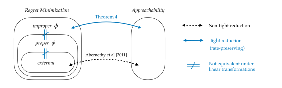
Figure 1: Overview of problem classes and reductions. Abernethy et al. (2011) give a non-tight reduction between approachability and external regret minimization. We give in Theorem 4 a tight (rate-preserving) reduction between approachability and the class of improper $\phi$-regret minimization problems. Further, we characterize when an improper $\phi$-regret instance is tightly reducible, under linear equivalence, to more well-studied classes of regret minimization problems, like proper $\phi$-regret minimization (Theorem 5) and external regret minimization (Theorem 6).

$\begin{aligned} \phi_{1}(p)&=(1,-p_{2},-2p_{3})\\ \phi_{2}(p)&=(0,2-p_{2},-2p_{3})\\ \phi_{3}(p)&=(0,-p_{2},3-2p_{3})\end{aligned}$	$\begin{aligned} \phi_{1}(p)&=(1,0,0)\\ \phi_{2}(p)&=(-p_{1},2-p_{2},-p_{3})\\ \phi_{3}(p)&=(-2p_{1},-2p_{2},3-2p_{3})\end{aligned}$	$\begin{aligned} \phi_{1}(p)&=(p_{1}-p_{2},p_{1}+p_{2},p_{3})\\ \phi_{2}(p)&=(p_{1}+p_{3},p_{2},p_{3}-p_{1})\\ \phi_{3}(p)&=(p_{1},p_{2}-p_{3},p_{2}+p_{3}).\end{aligned}$
(a)	(b)	(c)

Figure 2: Examples of improper $\phi$-regret minimization

1.2 Illustrative examples of improper $\phi$-regret and reductions

To illustrate the idea of linear equivalences between different regret minimization problems, in this section we present three different examples of $\phi$-regret minimization problems. All examples will have action set $\mathcal{P}=\Delta_{3}$ (the simplex over $3$ actions) and loss set $\mathcal{L}=[-1,1]^{d}$. The set of transformations $\Phi$ will always be of the form $\operatorname*{conv}(\{\phi_{1},\phi_{2},\phi_{3}\})$ but with these specific functions changing between examples as shown in Figure 2.

To begin, note that all these instances are truly improper $\phi$-regret problems; it is easy to find a $p=(p_{1},p_{2},p_{3})\in\Delta_{3}$ for which some $\phi_{i}(p)$ lies outside $\Delta_{3}$. Nonetheless, Blackwell approchability can be used to show that you can achieve sublinear $\phi$-regret for all three of these instances.

These three instances have different reducibility properties: instance (a) is linearly equivalent to an external regret problem, instance (b) is linearly equivalent to a proper $\phi$-regret problem (but not to any external regret problem), and instance (c) cannot be reduced to a proper $\phi$-regret problem.

To give an explicit example of what such a linear reduction entails, for instance (a), it turns out that for any $\ell\in\mathcal{L}$ and $p\in\mathcal{P}$ we have the equality $\langle p-\phi_{i}(p),\ell\rangle=\langle p-e_{i},\ell^{\prime}\rangle$, where $e_{i}$ is the $i$th basis vector and $\ell^{\prime}=\mathrm{diag}(1,1/2,1/3)\ell$. Therefore, this strange improper $\phi$-regret minimization problem is really an ordinary external regret minimization problem (on the modified loss set $\mathcal{L}^{\prime}=\mathrm{diag}(1,1/2,1/3)\mathcal{L}$) in disguise. One can also check that the different $\phi_{i}(p)$ differ by a constant, as required by our characterization.

Similarly, for instance (b), one can check that although the $\phi_{i}$ are improper, we can write $\langle p-\phi_{i}(p),\ell\rangle=\langle p-\phi^{\prime}_{i}(p),\ell^{\prime}\rangle$ for a set of proper $\phi^{\prime}_{i}$ and where $\ell^{\prime}=\ell/3$. On the other hand, there is no way to reduce this instance to an external regret instance, since different $\phi_{i}$ do not differ by a constant function. Interestingly, for this instance we can also write $\langle p-\phi_{i}(p),\ell\rangle=w_{i}\cdot\langle p-e_{i},\ell\rangle$ (for $(w_{1},w_{2},w_{3})=(1,2,3)$), showing that this instance captures a version of weighted external regret (where regret w.r.t action $i$ is multiplied by $w_{i}$). In particular, this demonstrates the (somewhat surprising fact) that weighted external regret cannot be written exactly as an external regret minimization problem.

Finally, instance (c) is an improper $\phi$-regret minimization problem that provably cannot be reduced to either of the smaller classes. Interestingly the construction of this $\phi$ comes from the fact that the skew-symmetric matrices of odd dimension form a linear subspace of singular matrices (each $p-\phi_{i}(p)$ is a skew-symmetric linear transformation).

1.3 Prior work

Blackwell’s approachability, applications and extensions.

There is a large body of work studying, extending, and applying Blackwell’s approachability theory to various problems of interest, including regret minimization (Foster and Vohra, 1999), game theory (Hart and Mas-Colell, 2000), reinforcement learning (Mannor and Shimkin, 2003; Kalathil et al., 2014; Miryoosefi et al., 2019), calibration (Dawid, 1982; Foster and Hart, 2018). Approachability and partial monitoring were studied in a series of publications by Perchet (2010); Mannor et al. (2014a, b); Perchet and Quincampoix (2015, 2018); Kwon and Perchet (2017). More recently, approachability has also been used in the analysis of fairness in machine learning (Chzhen et al., 2021). The notion of approachability has been extended in several studies. These include Vieille (1992) studying weak approachability in finite dimensional spaces, Spinat (2002) providing necessary and sufficient approachability conditions for arbitrary sets (not just convex sets), Lehrer (2003) extending approachability theory to infinite-dimensional spaces.

Improved regret guarantees through approachability for other norms.

As mentioned earlier, Abernethy et al. (2011) showed how to use Blackwell’s approachability to solve a general class of regret minimization problems. Nevertheless, their reduction could lead to suboptimal regret guarantees: e.g., a $\sqrt{TK}$ regret for an external regret minimization problem (with $T$ steps and $K$ actions), where $\sqrt{T\log(K)}$ is the optimal regret. It has been observed by many papers (Perchet, 2015; Shimkin, 2016; Kwon, 2021; Dann et al., 2023) since then that this is due to the choice of the $\ell_{2}$ norm for measuring the distance between the average payoff and the target set in approachability. With approachability algorithms for the more suitable $\ell_{\infty}$ norm, one can recover the optimal regret guarantees for many problems. Dann et al. (2023) address the time and space complexity of such algorithms from being prohibtibitely high: i.e., from not depending polynomially on the dimension of the space of vector payoffs.

Swap regret and repeated games.

The study of swap-regret and its generalizations has seen renewed interest in recent years due to its interesting connections to learning agents playing repeated games against strategic agents. While there is a large body of work on strategic agents playing against each other in repeated games, and also learning agents playing against each other in repeated games, the outcome of strategic agents playing against learners has remained largely unexplored until recently. The work of Deng, Schneider, and Sivan (2019) initiate the study of optimizer-learner interactions and show that a learner playing a no-swap-regret learning algorithm in a repeated game will not let an optimizer’s reward exceed the Stackelberg value of the game, where the latter itself is always obtainable by an optimizer playing against any no-regret learner. Mansour, Mohri, Schneider, and Sivan (2022) show that a learner playing a no-swap-regret algorithm is not just sufficient, but also necessary to ensure that an optimizer gets no more than the Stackelberg value of the game. They further study the class of Bayesian games and give a sufficient condition in the form of no-polytope-swap-regret for the optimizer to not exceed the Bayesian Stackelberg value of the game. This condition of no-polytope-swap-regret was shown to be necessary to cap the optimizer utility at the Bayesian Stackelberg value by Rubinstein and Zhao (2024). Special classes of these include (Braverman et al., 2018) studying the specific 2-player Bayesian game of an auction between a single seller and single buyer, Agrawal, Daskalakis, Mirrokni, and Sivan (2018) studying a similar setting but also other buyer behaviors beyond learning, and Cai, Weinberg, Wildenhain, and Zhang (2023) extending these to a single seller and multiple buyers.

$\Phi$-regret.

Several prominent notions of regret are special instances of $\Phi$-regret (Greenwald and Jafari, 2003). These include standard external regret, internal regret (Foster and Vohra, 1997) (see also (Stoltz and Lugosi, 2005, 2007; Greenwald et al., 2008)), and swap regret (Blum and Mansour, 2007; Peng and Rubinstein, 2023; Dagan et al., 2023). The notions of conditional swap regret (Mohri and Yang, 2014) or transductive regret (Mohri and Yang, 2017) are also related to $\Phi$-regret. Recently, $\Phi$-regret minimization has found applications in designing learning algorithms for extensive-form games that converge to certain classes of correlated equilibria (Celli et al., 2021; Bai et al., 2022; Zhang et al., 2024).

2 Model and Preliminaries

Given two convex sets $\mathcal{C}_{1}\subseteq\mathbb{R}^{d_{1}}$ and $\mathcal{C}_{2}\subseteq\mathbb{R}^{d_{2}}$, we define their tensor product $\mathcal{C}_{1}\otimes\mathcal{C}_{2}$ to be the subset of $\mathbb{R}^{d_{1}}\otimes\mathbb{R}^{d_{2}}\simeq\mathbb{R}^{d_{1}d_{2}}$ equal to the convex hull of all vectors of the form $c_{1}\otimes c_{2}=c_{1}c_{2}^{\top}$ for $c_{1}\in\mathcal{C}_{1}$ and $c_{2}\in\mathcal{C}_{2}$. We write $\mathsf{Lin}(\mathcal{C}_{1},\mathcal{C}_{2})$ to denote the collection of linear maps that send every point in $\mathcal{C}_{1}$ to a point in $\mathcal{C}_{2}$, and $\mathsf{Aff}(\mathcal{C}_{1},\mathcal{C}_{2})$ to denote the collection of affine maps that send every point in $\mathcal{C}_{1}$ to a point in $\mathcal{C}_{2}$. Note that if $\mathcal{C}_{1}$ belongs to an affine subspace of $\mathbb{R}^{d_{1}}$ (that does not contain the origin), then any affine function on $\mathcal{C}_{1}$ can be equivalently written as a linear function and so $\mathsf{Aff}(\mathcal{C}_{1},\mathcal{C}_{2})\simeq\mathsf{Lin}(\mathcal{C}_{1},\mathcal{C}_{2})$. On the other hand, if this is not the case, we can always augment $\mathcal{C}_{1}$ (by adding a $(d+1)$st dummy coordinate) and have that $\mathsf{Aff}(\mathcal{C}_{1},\mathcal{C}_{2})\simeq\mathsf{Lin}(\mathcal{C}^{\prime}_{1},\mathcal{C}_{2})$.

2.1 Approachability

An approachability problem is defined by three bounded convex subsets of Euclidean space: an action set $\mathcal{P}$, a loss set $\mathcal{L}$, and a “constraint” set of bi-affine functions $\mathcal{U}\subset\mathsf{Aff}(\mathcal{P}\otimes\mathcal{L},\mathbb{R})$. Traditionally, $\mathcal{U}$ is provided in the form of a multidimensional bilinear function ${\mathbf{u}}:\mathcal{P}\times\mathcal{L}\rightarrow\mathbb{R}^{n}$ (which would correspond to the $\mathcal{U}$ given by the convex hull of the $n$ components of ${\mathbf{u}}$), but it is easier and more general to work with $\mathcal{U}$ directly. For example, this lets us easily consider approachability problems with infinite-dimensional ${\mathbf{u}}$.

For a given time horizon $T$, an approachability algorithm $\mathcal{A}$ is a collection of functions $\{\mathcal{A}_{t}\}_{1\leq t\leq T}$, each of which takes as input a prefix of losses $\ell_{1},\ell_{2},\dots,\ell_{t-1}\in\mathcal{L}$ and returns an action $\mathcal{A}_{t}(\ell_{1},\dots,\ell_{t-1})=p_{t}$. For a given sequence of $T$ actions ${\mathbf{p}}$ and $T$ losses ${\bm{\ell}}$, we define the approachability loss $\operatorname{\mathsf{AppLoss}}({\mathbf{p}},{\bm{\ell}})$ to be

$$\operatorname{\mathsf{AppLoss}}({\mathbf{p}},{\bm{\ell}})=\max_{u\in\mathcal{U}}\sum_{t=1}^{T}u(p_{t},\ell_{t}).$$ (1)

The objective of an approachability problem is to construct approachability algorithms which guarantee low $\operatorname{\mathsf{AppLoss}}$. For a given algorithm $\mathcal{A}$ and time horizon $T$, let $\operatorname{\mathsf{AppLoss}}_{T}(\mathcal{A})$ be the worst-case approachability loss of $\mathcal{A}$ on any sequence of $T$ losses, that is, $\operatorname{\mathsf{AppLoss}}_{T}(\mathcal{A})=\max_{{\bm{\ell}}\in\mathcal{L}^{T}}\operatorname{\mathsf{AppLoss}}(\mathcal{A}({\bm{\ell}}),{\bm{\ell}})$. We will omit the subscript $T$ when it is clear from context.

We say an approachability instance $(\mathcal{P},\mathcal{L},\mathcal{U})$ is approachable if for each $\ell\in\mathcal{L}$, there exists a $p\in\mathcal{P}$ such that $u(p,\ell)\leq 0$ for all $u\in\mathcal{U}$. Blackwell’s theorem (Blackwell, 1956) provides the following dichotomy:

1. If an approachability instance $(\mathcal{P},\mathcal{L},\mathcal{U})$ is not approachable, then for any algorithm $\mathcal{A}$, $\operatorname{\mathsf{AppLoss}}_{T}(\mathcal{A})=\Omega(T)$.

2. If an approachability instance $(\mathcal{P},\mathcal{L},\mathcal{U})$ is approachable, then there exists an algorithm $\mathcal{A}$ where $\operatorname{\mathsf{AppLoss}}_{T}(\mathcal{A})=O(\sqrt{T})$.

For an approachable instance $(\mathcal{P},\mathcal{L},\mathcal{U})$, define

$$\operatorname{\mathsf{Rate}}(\mathcal{P},\mathcal{L},\mathcal{U})=\lim_{T\rightarrow\infty}\inf_{\mathcal{A}}\frac{\operatorname{\mathsf{AppLoss}}_{T}(\mathcal{A})}{\sqrt{T}}.$$ (2)

In words, the optimal algorithm for the instance $(\mathcal{P},\mathcal{L},\mathcal{U})$ achieves a worst-case approachability loss of $\operatorname{\mathsf{Rate}}(\mathcal{P},\mathcal{L},\mathcal{U})\sqrt{T}+o(\sqrt{T})$.

2.2 Regret minimization

Much like approachability problems, we specify a regret minimization problem by a triple of bounded convex sets: an action set $\mathcal{P}\subseteq\mathbb{R}^{d}$, a loss set $\mathcal{L}\subseteq\mathbb{R}^{d}$, and a benchmark set $\Phi\subseteq\mathsf{Aff}(\mathcal{P},\mathbb{R}^{d})$ of affine functions from $\mathcal{P}$ to $\mathbb{R}^{d}$). Intuitively, each function $\phi\in\Phi$ represents a “swap” or “transformation” function that the learner is competing against: if the learner outputs a sequence of actions $p_{1},p_{2},\dots,p_{T}$, they want to have low regret compared to the sequence of actions $\phi(p_{1}),\phi(p_{2}),\dots,\phi(p_{T})$.

For a given regret minimization instance $(\mathcal{P},\mathcal{L},\Phi)$, the regret of a sequence of $T$ actions ${\mathbf{p}}$ and $T$ losses ${\bm{\ell}}$ is given by

$$\operatorname{\mathsf{Reg}}({\mathbf{p}},{\bm{\ell}})=\max_{\phi\in\Phi}\left(\sum_{t=1}^{T}\langle p_{t},\ell_{t}\rangle-\sum_{t=1}^{T}\langle\phi(p_{t}),\ell_{t}\rangle\right).$$ (3)

As with approachability, our goal is to design a learning algorithm $\mathcal{A}$ for this problem which achieves low worst-case regret. In fact, it is fairly straightforward to write the above regret minimization problem as a specific instance of approachability: let $\mathcal{U}$ be the set of bilinear functions of the form

$$u_{\phi}(p,\ell)=\langle p,\ell\rangle-\langle\phi(p),\ell\rangle,$$ (4)

where $\phi$ ranges over all $\phi\in\Phi$, then it is easy to see that the expression for $\operatorname{\mathsf{Reg}}({\mathbf{p}},{\bm{\ell}})$ in (3) is equivalent to the expression for $\operatorname{\mathsf{AppLoss}}({\mathbf{p}},{\bm{\ell}})$ in (1). We will likewise write $\operatorname{\mathsf{Reg}}_{T}(\mathcal{A})$ to refer to the worst-case regret of algorithm $\mathcal{A}$, and $\operatorname{\mathsf{Rate}}(\mathcal{P},\mathcal{L},\Phi)$ to represent the optimal regret rate for this regret minimization instance.

If each $\phi\in\Phi$ contains a fixed point in $\mathcal{P}$, then the corresponding approachability problem is approachable and $\operatorname{\mathsf{Rate}}(\mathcal{P},\mathcal{L},\Phi)<\infty$. Furthermore, if the loss set $\mathcal{L}$ contains a vector in every direction ($\operatorname*{cone}(\mathcal{L})=\mathbb{R}^{d}$), then this condition exactly characterizes regret minimization instances that permit sublinear regret algorithms.

Theorem 1.

Consider a regret minimization instance $(\mathcal{P},\mathcal{L},\Phi)$. If each $\phi\in\Phi$, has a fixed point $p_{\phi}\in\mathcal{P}$ (i.e., $\phi(p_{\phi})=p_{\phi}$), then $\operatorname{\mathsf{Rate}}(\mathcal{P},\mathcal{L},\Phi)<\infty$. Conversely, if $\operatorname*{cone}(\mathcal{L})=\mathbb{R}^{d}$ and $\operatorname{\mathsf{Rate}}(\mathcal{P},\mathcal{L},\Phi)<\infty$, then every $\phi\in\Phi$ must have a fixed point in $\mathcal{P}$.

Proof.

To prove the forward direction, we will prove the corresponding approachability problem (defined via (4)) is approachable. For this, we must show that for any $\phi\in\Phi$, there exists a $p\in\mathcal{P}$ such that $u_{\phi}(p,\ell)\leq 0$ for all $\ell\in\mathcal{L}$. But since $u_{\phi}(p,\ell)=\langle p-\phi(p),\ell\rangle$, if we take $p=p_{\phi}$, $p_{\phi}-\phi(p_{\phi})=0$ and $u_{\phi}(p,\ell)=0$ for all $\ell\in\mathcal{L}$.

Conversely, assume there exists a $\phi\in\Phi$ without a fixed point. Consider the set $V=\{p-\phi(p)\mid p\in\mathcal{P}\}$. $V$ is a convex bounded set (since it is a linear transformation of $\mathcal{P}$ that by assumption does not contain $0$. Therefore, there exists a hyperplane separating $V$ from $0$ – in particular, there exists a $w$ such that $\langle v,w\rangle>0$ for any $v\in V$. If we take $\ell$ proportional to $w$ (possible since $\operatorname*{cone}(\mathcal{L})=\mathbb{R}^{d}$), then for this $\phi$ and $\ell$, there is no $p\in\mathcal{P}$ such that $u_{\phi}(p,\ell)\leq 0$. It follows that the corresponding approachability problem is not approachable, and therefore $\operatorname{\mathsf{Rate}}(\mathcal{P},\mathcal{L},\Phi)=\infty$. ∎

We will categorize regret minimization instances into three classes based on the properties of their set of benchmarks $\Phi$, which we list in increasing order of generality:

• External regret minimization. If each $\phi\in\Phi$ has the property that $\phi$ is a constant function over $\mathcal{P}$ (i.e., there exists a $p_{\phi}\in\mathcal{P}$ s.t. $\phi(p)=p_{\phi}$ for all $p\in\mathcal{P}$), then we say that this instance of regret minimization is an external regret minimization instance. Note that the classic online learning setting of online linear optimization fits into this class (the benchmark set $\Phi$ is the set of all constant functions on $\mathcal{P}$).

• Proper $\phi$-regret minimization. If each $\phi\in\Phi$ has the property that $\phi(p)\in\mathcal{P}$ whenever $p\in\Phi$ (i.e., each $\phi$ maps $\mathcal{P}$ into itself), then we say that this instance of regret minimization is a proper $\phi$-regret minimization instance. Note that by Brouwer’s fixed-point theorem, each $\phi$ must contain a fixed point in $\mathcal{P}$, and therefore each proper $\phi$-regret minimization problem has a sublinear-regret algorithm.

  This class captures the well-known cases of swap regret and internal regret, along with the notion of linear $\phi$-regret studied in (Gordon et al., 2008). It also contains the previous class of external regret minimization instances.

• Improper $\phi$-regret minimization. As long as each $\phi\in\Phi$ has a fixed point in $\mathcal{P}$ (a $p\in\mathcal{P}$ s.t. $\phi(p)=p$), we say that this instance of regret minimization is an improper $\phi$-regret instance.

  Note here that the benchmark functions $\phi$ are allowed to send points in $\mathcal{P}$ to points outside of $\mathcal{P}$ (that the learner is not even allowed to play). Nonetheless, by Theorem 1, we know that $\operatorname{\mathsf{Rate}}(\mathcal{P},\mathcal{L},\Phi)<\infty$ for any such improper $\phi$-regret instance.

2.3 Reductions between learning problems

Ideally, we would design efficient learning algorithms that provably match the optimal rate for a given approachability or regret minimization instance. Unfortunately, doing this directly seems very challenging – even for the special case of online linear optimization, it is unclear how to construct efficient learning algorithms with near-optimal regret bounds.

Instead, we will settle for being able to reduce an arbitrary approachability instance $(\mathcal{P},\mathcal{L},\mathcal{U})$ to an instance of a simpler learning problem. In particular, all of our simpler learning problems we consider can also be written as approachability problems, so our main goal is to understand when a specific approachability instance $(\mathcal{P},\mathcal{L},\mathcal{U})$ is “reducible” to a second specific instance $(\mathcal{P}^{\prime},\mathcal{L}^{\prime},\mathcal{U}^{\prime})$.

We define our notion of reducibility as follows. We say there is a tight reduction between instance $\mathcal{I}=(\mathcal{P},\mathcal{L},\mathcal{U})$ and instance $\mathcal{I}^{\prime}=(\mathcal{P}^{\prime},\mathcal{L}^{\prime},\mathcal{U}^{\prime})$ if both: i. given any algorithm $\mathcal{A}$ for $\mathcal{I}$, we can construct an algorithm $\mathcal{A}^{\prime}$ for $\mathcal{I}^{\prime}$ with $\operatorname{\mathsf{AppLoss}}(\mathcal{A}^{\prime})=\operatorname{\mathsf{AppLoss}}(\mathcal{A})$, and ii. given any algorithm $\mathcal{A}^{\prime}$ for $\mathcal{I}^{\prime}$, we can construct an algorithm $\mathcal{A}$ for $\mathcal{I}$ with $\operatorname{\mathsf{AppLoss}}(\mathcal{A})=\operatorname{\mathsf{AppLoss}}(\mathcal{A}^{\prime})$. We say there is a $c$-approximate reduction between the two instances if, for sufficiently large $T$, we instead have $\operatorname{\mathsf{AppLoss}}(\mathcal{A}^{\prime})\leq c\operatorname{\mathsf{AppLoss}}(\mathcal{A})$ and $\operatorname{\mathsf{AppLoss}}(\mathcal{A})\leq c\operatorname{\mathsf{AppLoss}}_{T}(\mathcal{A}^{\prime})$ in the two constraints respectively. Finally, we say that there is a weak reduction from instance $\mathcal{I}$ to instance $\mathcal{I}^{\prime}$ if we only have one direction of the reduction: given an algorithm $\mathcal{A}^{\prime}$ for $\mathcal{I}^{\prime}$, we can efficiently construct an algorithm $\mathcal{A}$ for $\mathcal{I}$ with $\operatorname{\mathsf{AppLoss}}(\mathcal{A})\leq\operatorname{\mathsf{AppLoss}}(\mathcal{A}^{\prime})$. Note that a tight reduction implies that $\operatorname{\mathsf{Rate}}(\mathcal{I}^{\prime})=\operatorname{\mathsf{Rate}}(\mathcal{I})$, a $c$-approximate reduction implies that $\operatorname{\mathsf{Rate}}(\mathcal{I})/c\leq\operatorname{\mathsf{Rate}}(\mathcal{I}^{\prime})\leq c\operatorname{\mathsf{Rate}}(\mathcal{I})$, and a weak reduction from $\mathcal{I}$ to $\mathcal{I}^{\prime}$ only implies that $\operatorname{\mathsf{Rate}}(\mathcal{I})\leq\operatorname{\mathsf{Rate}}(\mathcal{I}^{\prime})$.

Since any regret minimization instance can be written as an approachability instance, we can use the same notion of reducibility when talking about reductions among instances of regret minimization. The latter sections of this paper will be concerned with understanding when a specific instance of approachability is equivalent to an instance of a specific class of regret minimization problems. There we will use a more restrictive notion of “linear equivalence”, where all relevant constructions must be provided by affine transformations; we introduce this in Section 4.

2.4 The classical reduction from approachability to external regret minimization

Finally, we present the classical reduction from approachability to external regret minimization. This is the same reduction in (Abernethy et al., 2011) (and subsequent works), adapted to our notation.

Theorem 2.

[ Abernethy et al. (2011)] Given any instance $\mathcal{I}=(\mathcal{P},\mathcal{L},\mathcal{U})$ of approachability, there exists a weak reduction from $\mathcal{I}$ to an instance $\mathcal{I}^{\prime}=(\mathcal{P}^{\prime},\mathcal{L}^{\prime},\Phi^{\prime})$ of external regret minimization.

Proof.

We will define the target instance $\mathcal{I}^{\prime}$ as follows. We will let the new action set $\mathcal{P}^{\prime}=\mathcal{U}$ and the new loss set $\mathcal{L}^{\prime}=-(\mathcal{P}\otimes\mathcal{L})$. Note that both $\mathcal{P}^{\prime}$ and $\mathcal{L}^{\prime}$ are convex subsets of $(\dim\mathcal{P})(\dim\mathcal{L})$-dimensional Euclidean space, and we can define a bilinear pairing between $\mathcal{P}^{\prime}$ and $\mathcal{L}^{\prime}$ via $\langle u,-(p\otimes\ell)\rangle=-u(p,\ell)$ for any $u\in\mathcal{P}^{\prime}$ and $-(p\otimes\ell)\in\mathcal{L}^{\prime}$. Finally, we will let the new benchmark set $\mathcal{U}^{\prime}$ consist of all constant functions over $\mathcal{P}^{\prime}$ (i.e., for each $x\in\mathcal{P}^{\prime}$, there will exist a $u^{\prime}_{x}\in\mathcal{U}^{\prime}$ such that $u^{\prime}_{x}(p^{\prime})=x$ for all $p^{\prime}\in\mathcal{P}^{\prime}$). In other words, $\mathcal{I}^{\prime}$ is the online linear optimization problem with action set $\mathcal{P}^{\prime}$ and loss set $\mathcal{L}^{\prime}$ (and is an external regret minimization problem).

Given a low-regret algorithm $\mathcal{B}$ for solving $\mathcal{I}^{\prime}$, we construct the following algorithm $\mathcal{A}$ for solving $\mathcal{I}$ using $\mathcal{B}$ as a black box. In round $t$:

1. Set $p^{\prime}_{t}=\mathcal{B}_{t}(\ell^{\prime}_{1},\ell^{\prime}_{2},\dots,\ell^{\prime}_{t-1})\in\mathcal{P}^{\prime}$.

2. Play $p_{t}\in\mathcal{P}$ s.t. $\langle p^{\prime}_{t},p_{t}\otimes\ell\rangle\leq 0$ for all $\ell\in\mathcal{L}$. Note that such a $p_{t}$ exists since the instance $(\mathcal{P},\mathcal{L},\mathcal{U})$ is approachable – in particular, $\langle p^{\prime}_{t},p_{t}\otimes\ell\rangle=p^{\prime}_{t}(p_{t},\ell)$ for some $p^{\prime}_{t}\in\mathcal{U}$, and the approachability condition implies that there must exist a $p_{t}$ where $p^{\prime}_{t}(p_{t},\ell)\leq 0$ for all $\ell\in\mathcal{L}$.

3. Receive the loss $\ell_{t}$.

4. Set $\ell^{\prime}_{t}=-(p_{t}\otimes\ell_{t})\in\mathcal{L}^{\prime}$.

By the definition of $\operatorname{\mathsf{Reg}}({\mathbf{p}}^{\prime},{\bm{\ell}}^{\prime})$, we have

$$\operatorname{\mathsf{Reg}}({\mathbf{p}}^{\prime},{\bm{\ell}}^{\prime}) =\sum_{t=1}^{T}\langle p^{\prime}_{t},\ell^{\prime}_{t}\rangle-\min_{x^{*}\in\mathcal{P}^{\prime}}\sum_{t=1}^{T}\langle x^{*},\ell^{\prime}_{t}\rangle$$

$$=\sum_{t=1}^{T}\langle p^{\prime}_{t},-(p_{t}\otimes\ell_{t})\rangle-\min_{u^{*}\in\mathcal{U}}\sum_{t=1}^{T}\langle u^{*},-(p_{t}\otimes\ell_{t})\rangle$$

$$=\max_{u^{*}\in\mathcal{U}}\sum_{t=1}^{T}u^{*}(p_{t},\ell_{t})-\sum_{t=1}^{T}p^{\prime}_{t}(p_{t},\ell_{t})$$

$$=\operatorname{\mathsf{AppLoss}}({\mathbf{p}},{\bm{\ell}})-\sum_{t=1}^{T}p^{\prime}_{t}(p_{t},\ell_{t})\geq\operatorname{\mathsf{AppLoss}}({\mathbf{p}},{\bm{\ell}}).$$

This very final inequality follows from the fact that $p^{\prime}_{t}(p_{t},\ell)\leq 0$ for all $\ell\in\mathcal{L}$ via our choice of $p_{t}$ in step 2. Altogether, this analysis implies that $\operatorname{\mathsf{AppLoss}}(\mathcal{A})\leq\operatorname{\mathsf{Reg}}(\mathcal{B})$, and therefore provides a weak reduction from $\mathcal{I}$ to $\mathcal{I}^{\prime}$. ∎

3 Reducing approachability to (improper) regret minimization

3.1 The classical reduction is not tight

Theorem 2 proves that the classical reduction of Abernethy et al. (2011) is a weak reduction from any approachability problem to an external regret minimization problem. It is natural to wonder whether this reduction is in fact tight, or if not, whether the gap in rates between the original approachability problem and the eventual regret problem is small. The following counterexample proves that this is not the case.

Theorem 3.

There exists an approachability instance $\mathcal{I}$ such that $\operatorname{\mathsf{Rate}}(\mathcal{I})=0$ but $\operatorname{\mathsf{Rate}}(\mathcal{I}^{\prime})>0$, where $\mathcal{I}^{\prime}$ is the regret minimization instance obtained by applying the reduction of Theorem 2 to $\mathcal{I}$. In particular, there is no finite $c>0$ for which the reduction in Theorem 2 is a $c$-approximate reduction for all approachability instances, and the reduction is not tight.

Proof.

Consider the following approachability instance $\mathcal{I}$. Fix any $d^{\prime}\geq 2$ and let $d=d^{\prime}+1$. We will let $\mathcal{P}=\Delta_{d}$, $\mathcal{L}=[0,1]^{d}$, and $\mathcal{U}$ to be the convex hull of the $d^{\prime}$ bilinear functions $u_{i}$, where for $i\in[d^{\prime}]$,

$$u_{i}(p,\ell)=\sum_{j=1}^{d^{\prime}}p_{j}(\ell_{j}-\ell_{i}).$$

Here the $u_{i}$ constraint for $i\in[d^{\prime}]$ can be thought of as the regret of moving all probability mass on $p_{1}$ through $p_{d^{\prime}}$ to $p_{i}$. Note, however, that the learner also has the option of placing probability mass on action $d^{\prime}+1$, which has no approachability constraint associated with this. As a result, $\operatorname{\mathsf{Rate}}(\mathcal{I})=0$, since the learner can perfectly approach the negative orthant by always playing $p_{t}=e_{d^{\prime}+1}$.

However, the instance of external regret minimization we reduce to will have a worse rate, as it will require solving a genuine regret minimization problem. Let $\mathcal{I}^{\prime}=(\mathcal{P}^{\prime},\mathcal{L}^{\prime},\Phi^{\prime})$ be the regret minimization instance formed by applying the reduction of Theorem 2. This instance has $\mathcal{P}^{\prime}=\mathcal{U}$, $\mathcal{L}^{\prime}=-(\mathcal{P}\otimes\mathcal{L})$, and $\mathcal{U}^{\prime}$ the set of all constant functions on $\mathcal{P}^{\prime}$. We will restrict the loss set further, and insist that the only losses $\ell^{\prime}_{t}$ are of the form $\ell^{\prime}_{t}=-(U_{d^{\prime}}\otimes\ell_{t})$, where $U_{d^{\prime}}=(1/d^{\prime},1/d^{\prime},\dots,1/d^{\prime},0)\in\mathcal{P}$ is the uniform distribution over the first $d^{\prime}$ coordinates, and $\ell_{t}$ is chosen from the subset $\mathcal{L}_{2}\subseteq\mathcal{L}$ containing all elements of $\mathcal{L}$ whose last coordinate equals $0$ (so $\mathcal{L}_{2}\cong[0,1]^{d^{\prime}}$). Since this restricts the adversary, it only makes the regret minimization problem easier (and the rate smaller).

The regret of a pair of sequences ${\mathbf{p}}^{\prime}$ and ${\bm{\ell}}^{\prime}$ for this new problem can be written as

$$\operatorname{\mathsf{Reg}}({\mathbf{p}}^{\prime},{\bm{\ell}}^{\prime})=\max_{x^{*}\in\mathcal{P}^{\prime}}\left(\sum_{t=1}^{T}\langle p^{\prime}_{t},\ell^{\prime}_{t}\rangle-\sum_{t=1}^{T}\langle x^{*},\ell^{\prime}_{t}\rangle\right).$$ (5)

To simplify this further, note that the set $\mathcal{P}^{\prime}=\mathcal{U}$ is given by the convex hull of the $d^{\prime}$ bilinear functions $u_{i}$, so we can write each element of $\mathcal{P}^{\prime}$ uniquely as a convex combination of these $d^{\prime}$ functions. For a $p^{\prime}\in\mathcal{P}^{\prime}$, we will write $p^{\prime}_{i}$ to be the coefficient of $u_{i}$ in this convex combination (in this way, we identify $\mathcal{P}^{\prime}$ with the simplex $\Delta_{d^{\prime}}$).

Now, for any $p^{\prime}\in\mathcal{P}^{\prime}$ and $\ell^{\prime}\in\mathcal{L}^{\prime}$ (of the above restricted form), we can write

$$\langle p^{\prime},\ell^{\prime}\rangle=-\sum_{i=1}^{d^{\prime}}p^{\prime}_{i}\left(\frac{1}{d^{\prime}}\sum_{j=1}^{d^{\prime}}(\ell_{j}-\ell_{i})\right)=\left\langle p^{\prime},\pi(\ell)\right\rangle-\frac{1}{d^{\prime}}\left(\sum_{i=1}^{d^{\prime}}\pi(\ell)_{i}\right),$$ (6)

where $\pi(\ell)$ is the projection of $\ell$ onto the first $d^{\prime}$ coordinates. Substituting this in turn into (5) yields

$$\operatorname{\mathsf{Reg}}({\mathbf{p}}^{\prime},{\bm{\ell}}^{\prime})=\max_{x^{*}\in\mathcal{P}^{\prime}}\left(\sum_{t=1}^{T}\langle p^{\prime}_{t},\pi(\ell_{t})\rangle-\sum_{t=1}^{T}\left\langle x^{*},\pi(\ell_{t})\right\rangle\right).$$ (7)

Now, note that the adversary can choose $\ell_{t}$ so that $\pi(\ell_{t})$ takes on any value in $\mathcal{L}_{2}=[0,1]^{d^{\prime}}$. Similarly, $p^{\prime}$ can take on any value in $\mathcal{P}_{2}=\mathcal{P}^{\prime}=\Delta_{d^{\prime}}$. Therefore, this problem is at least as hard as the online linear optimization problem with action set $\mathcal{P}_{2}=\Delta_{d_{2}}$ and loss set $\mathcal{L}_{2}=[0,1]^{d_{2}}$. But this is exactly the online learning with experts problem (with $d^{\prime}$ experts), which has a regret lower bound of $\Omega(\sqrt{T\log d^{\prime}})$. It follows that $\operatorname{\mathsf{Rate}}(\mathcal{I}^{\prime})\geq\Omega(\sqrt{\log d^{\prime}})>0$. ∎

One may object that the approachability instance in the proof of Theorem 3 is somewhat degenerate, since the approachability instance has a clear optimal action for the learner (which guarantees perfect approachability). In Appendix B we show that it is possible to slightly perturb this example in a way that avoids the existence of such an optimal action, while maintaining an arbitrarily large gap in rates between the two instances.

3.2 A tight reduction from approachability to improper $\phi$-regret minimization

In contrast to Theorem 3, it turns out that it is possible to tightly reduce approachability to improper $\phi$-regret. The key observation is that if we “augment” the action space of the learner as to also include the benchmark $u\in\mathcal{U}$ they are competing against each round, we can directly interpret $\operatorname{\mathsf{AppLoss}}({\mathbf{p}},{\bm{\ell}})$ as a specific $\phi$-regret on this space.

Theorem 4.

For any approachability instance $\mathcal{I}=(\mathcal{P},\mathcal{L},\mathcal{U})$, there exists a tight reduction from $\mathcal{I}$ to an improper $\phi$-regret minimization instance $\mathcal{I}^{\prime}=(\mathcal{P}^{\prime},\mathcal{L}^{\prime},\Phi^{\prime})$.

Proof.

Let $\mathcal{X}=\mathcal{U}\otimes\mathcal{P}$ and $\mathcal{Y}=\mathcal{L}$. Let $B(x,y):\mathcal{X}\times\mathcal{Y}\rightarrow\mathbb{R}$ be the bilinear form defined via $B(u\otimes p,\ell)=-u(p,\ell)$. Note that we can write

$$\operatorname{\mathsf{AppLoss}}({\mathbf{p}},{\bm{\ell}}) =\max_{u\in\mathcal{U}}\sum_{t=1}^{T}u(p_{t},\ell_{t})$$

$$=\max_{u\in\mathcal{U}}\sum_{t=1}^{T}-B(u\otimes p_{t},\ell_{t})$$

$$=\max_{u\in\mathcal{U}}\left(\sum_{t=1}^{T}B(x_{t},\ell_{t})-\sum_{t=1}^{T}B(\phi_{u}(x_{t}),\ell_{t})\right),$$

where $\phi_{u}:\mathcal{X}\rightarrow\mathcal{X}$ is the linear function defined via $\phi_{u}(u^{\prime}\otimes p)=u\otimes p$ (for any $u^{\prime}\in\mathcal{U}$). Now, the bilinear form $B$ corresponds to a matrix $M_{B}$ such that $B(x,y)=\langle x,M_{B}y\rangle$. From this it follows that if we set $\mathcal{P}^{\prime}=\mathcal{X}$, $\mathcal{L}^{\prime}=M_{B}\mathcal{Y}$, and $\Phi^{\prime}=\{\phi_{u}\mid u\in\mathcal{U}\}$, then $\operatorname{\mathsf{AppLoss}}({\mathbf{p}},{\bm{\ell}})=\operatorname{\mathsf{Reg}}({\mathbf{p}}^{\prime},{\bm{\ell}}^{\prime})$ and this is a tight reduction between $\mathcal{I}$ and $\mathcal{I}^{\prime}$. ∎

Theorem 4 prompts us to question when we can further reduce an improper $\phi$-regret minimization instance to a proper one. We study this question through the lens of linear equivalence in the next section.

4 Tight linear reductions for regret minimization

4.1 Warm-up: weighted regret minimization

Theorem 4 implies that approachability is equivalent to improper $\phi$-regret minimization. Ideally, we would be able to, in turn, tightly reduce this instance of improper $\phi$-regret minimization to an instance of the better studied problem of external regret minimization (as the classical reduction attempts to do), or at least to an instance of proper $\phi$-regret minimization.

In this section, we examine the question of “which instances of regret minimization are tightly reducible to each other?”, and specifically “when is an improper $\phi$-regret instance tightly reducible to a proper $\phi$-regret (or even an external regret) instance?”. However, the space of general reductions is hard to work with directly – for this reason, we will restrict ourselves to a subclass of these reductions that we call linear equivalences. We will formally define linear equivalences in the next section. For now, we will begin by motivating them via an application where a non-trivial tight reduction is possible: solving the problem of weighted regret minimization.

In the weighted regret minimization problem, we have an action set $\mathcal{P}$, a loss set $\mathcal{L}$, and a collection $\Phi=\{\phi_{1}(p),\phi_{2}(p),\dots,\phi_{N}(p)\}$ of proper affine benchmark functions (i.e., each $\phi_{i}$ maps $\mathcal{P}$ to itself). Each $\phi_{i}$ has an accompanying scalar weight $w_{i}>0$, representing the importance we place on regret with respect to $\phi_{i}$. As with the general regret minimization problem and approachability problem, the learner runs a learning algorithm to decide their action at time $t$. The goal of the learner is to minimize the expression:

$$\operatorname{\mathsf{WReg}}({\mathbf{p}},{\bm{\ell}})=\max_{i\in[N]}\left(w_{i}\cdot\left[\sum_{t=1}^{T}\langle p,\ell\rangle-\sum_{t=1}^{T}\langle\phi_{i}(p),\ell\rangle\right]\right).$$ (8)

In other words, $\operatorname{\mathsf{WReg}}({\mathbf{p}},\ell)$ simply equals the corresponding $\phi$-regret where the regret with respect to $\phi_{i}$ is scaled by $w_{i}$.

One way to approach a specific weighted regret minimization problem $\mathcal{I}$ is to simply ignore the weights and run an algorithm for the corresponding proper $\phi$-regret minimization problem. This would work, in the sense that a sublinear regret algorithm for the unweighted problem would also obtain sublinear regret for the weighted regret minimization problem. But completely ignoring the weights is, of course, lossy: a regret guarantee of $R$ for the unweighted problem only translates to a regret guarantee of $(\max w_{i})R$ for the weighted problem. Conversely, if we have a learning algorithm with a regret guarantee of $R$ for the weighted problem, running it on the unweighted instance only translates to a regret guarantee of $R/(\min w_{i})$. In the language of our different types of reductions, this naive translation of algorithms is only an $\omega$-approximate reduction, where $\omega=(\max w_{i})/(\min w_{i})$.

Despite this, it is possible to exactly write the weighted regret minimization problem as a regret minimization problem of the form described in Section 2.2. We simply need to observe that:

$$w_{i}\left(\langle p,\ell\rangle-\langle\phi_{i}(p),\ell\rangle\right)=\langle p,\ell\rangle-\left\langle w_{i}\phi_{i}(p)-(w_{i}-1)p,\ell\right\rangle.$$ (9)

Therefore, if we let $\widetilde{\phi}_{i}(p)=w_{i}\phi_{i}(p)-(w_{i}-1)p$ and $\widetilde{\Phi}=\operatorname*{conv}(\{\widetilde{\phi}_{i}\}_{i=1}^{N})$, then the regret minimization instance $(\mathcal{P},\mathcal{L},\widetilde{\Phi})$ is exactly equivalent to our weighted regret minimization problem. However, this regret minimization problem is in general an improper $\phi$-regret minimization problem (even though all the original $\phi_{i}$ are proper). In fact, this is the case even when the benchmarks $\phi_{i}$ are all constant and correspond to a weighted external regret minimization problem (e.g., if $\mathcal{P}=\Delta_{3}$, $\phi_{1}(p)=(1,0,0)$, and $w_{1}=2$, then $\widetilde{\phi}_{1}(p)=(2-p_{1},-p_{2},-p_{3})$).

It turns out that in this case, there is a tight reduction between this improper $\phi$-regret minimization problem and a proper $\phi$-regret minimization problem.

Theorem 5.

There exists a tight reduction from the improper $\phi$-regret instance $\mathcal{I}=(\mathcal{P},\mathcal{L},\widetilde{\Phi})$ to a proper $\phi$-regret instance $\mathcal{I}^{\prime}$.

Proof.

We can construct the proper $\phi$-regret minimization problem as follows. Let $W=\max w_{i}$, and let $\mathcal{P}^{\prime}=\mathcal{P}$, $\mathcal{L}^{\prime}=W\mathcal{L}$, and $\Phi^{\prime}=\operatorname*{conv}(\{\phi^{\prime}_{i}\}_{i=1}^{N})$, where

$$\phi^{\prime}_{i}(p)=\frac{w_{i}}{W}\phi_{i}(p)+\left(1-\frac{w_{i}}{W}\right)p.$$

Note that each $\phi^{\prime}_{i}$ is the convex combination of the two proper functions $\phi_{i}$ and the identity, and is therefore also proper. We let $\mathcal{I}^{\prime}=(\mathcal{P}^{\prime},\mathcal{L}^{\prime},\Phi^{\prime})$ denote this proper $\phi$-regret minimization problem.

The reduction from $\mathcal{I}$ to $\mathcal{I}^{\prime}$ is very simple and boils down to rescaling the losses by $W$. The necessary observation is just that:

$$\langle p-\widetilde{\phi}_{i}(p),\ell\rangle=\langle p-\phi^{\prime}_{i}(p),W\ell\rangle.$$ (10)

In particular, given an algorithm $\mathcal{A}^{\prime}$ for $\mathcal{I}^{\prime}$, we can construct an algorithm $\mathcal{A}$ for $\mathcal{I}$ with $\operatorname{\mathsf{Reg}}(\mathcal{A}^{\prime})=\operatorname{\mathsf{Reg}}(\mathcal{A})$ as follows:

1. At the beginning of round $t$, $\mathcal{A}$ asks $\mathcal{A}^{\prime}$ for the $p^{\prime}_{t}$ it will play. $\mathcal{A}$ then plays $p_{t}=p^{\prime}_{t}$.

2. $\mathcal{A}$ observes their loss vector $\ell_{t}$. $\mathcal{A}$ passes along the loss vector $\ell^{\prime}_{t}=W\ell_{t}$ to $\mathcal{A}^{\prime}$.

Equation (10) implies that not only do the worst-case regrets $\operatorname{\mathsf{Reg}}(\mathcal{A}^{\prime})=\operatorname{\mathsf{Reg}}(\mathcal{A})$ agree for the above pair of algorithms, but that in any execution of the reduction, both algorithms achieve exactly the same regret. A similar reduction (dividing the loss by $W$ instead of multiplying it by $W$) suffices to show that we can transform an algorithm $\mathcal{A}$ for $\mathcal{I}$ to an algorithm $\mathcal{A}^{\prime}$ for $\mathcal{I}^{\prime}$ with the same regret bound. ∎

4.2 Linear equivalences

Motivated by the reduction in Theorem 5, we introduce the following notion of a “linear equivalence” between two regret minimization problems. In short, a linear equivalence will be a tight reduction between two regret minimization instances with the property that the reduction is given entirely by linear transformations.

Formally, let $\mathcal{I}=(\mathcal{P},\mathcal{L},\Phi)$ be a regret minimization instance with $\dim(\mathcal{P})=\dim(\mathcal{L})=d$. We say that there is a linear equivalence between this instance and the instance $\mathcal{I}^{\prime}=(\mathcal{P},\mathcal{L}^{\prime},\Phi^{\prime})$ if there exists a bijective correspondence between $\phi\in\Phi$ and $\phi^{\prime}\in\Phi^{\prime}$ such that the following conditions hold:

• There exist affine maps $S_{\mathcal{P}^{\prime},\mathcal{P}}\in\mathsf{Aff}(\mathcal{P}^{\prime},\mathcal{P})$ and $S_{\mathcal{L},\mathcal{L}^{\prime}}\in\mathsf{Aff}(\mathcal{L},\mathcal{L}^{\prime})$, such that for any $\ell\in\mathcal{L}$, $p^{\prime}\in\mathcal{P}^{\prime}$, $\ell^{\prime}=S_{\mathcal{L},\mathcal{L}^{\prime}}\ell$, and $p=S_{\mathcal{P}^{\prime},\mathcal{P}}p^{\prime}$, we have:

  $$\langle p-\phi(p),\ell\rangle=\langle p^{\prime}-\phi^{\prime}(p^{\prime}),\ell^{\prime}\rangle.$$ (11)

• There exist affine maps $S_{\mathcal{P},\mathcal{P}^{\prime}}\in\mathsf{Aff}(\mathcal{P},\mathcal{P}^{\prime})$ and $S_{\mathcal{L}^{\prime},\mathcal{L}}\in\mathsf{Aff}(\mathcal{L}^{\prime},\mathcal{L})$ such that for any $\ell^{\prime}\in\mathcal{L}^{\prime}$, $p\in\mathcal{P}$, $\ell=S_{\mathcal{L}^{\prime},\mathcal{L}}\ell^{\prime}$ and $p^{\prime}=S_{\mathcal{P},\mathcal{P}^{\prime}}p$, we have:

  $$\langle p-\phi(p),\ell\rangle=\langle p^{\prime}-\phi^{\prime}(p^{\prime}),\ell^{\prime}\rangle.$$ (12)

Note that the first point above has the following implication. If you have a learning algorithm $\mathcal{A}^{\prime}$ for $\mathcal{I}^{\prime}$, you can use it to construct a learning algorithm $\mathcal{A}$ for $\mathcal{I}$ by following the procedure:

1. At the beginning of round $t$, $\mathcal{A}$ asks $\mathcal{A}^{\prime}$ for the $p^{\prime}_{t}$ it will play.

2. $\mathcal{A}$ then plays $p_{t}=S_{\mathcal{P}^{\prime},\mathcal{P}}p^{\prime}_{t}$.

3. $\mathcal{A}$ observes their loss vector $\ell_{t}$.

4. $\mathcal{A}$ passes along the loss vector $\ell^{\prime}_{t}=S_{\mathcal{L},\mathcal{L}^{\prime}}\ell_{t}$ to $\mathcal{A}^{\prime}$.

The guarantee of equation (11) implies that $\operatorname{\mathsf{Reg}}_{T}(\mathcal{A})\leq\operatorname{\mathsf{Reg}}_{T}(\mathcal{A}^{\prime})$. Likewise, the guarantee of equation (12) (and its surrounding bullet) implies that given an algorithm $\mathcal{A}$ for $\mathcal{I}$, we can efficiently construct an algorithm $\mathcal{A}^{\prime}$ for $\mathcal{I}^{\prime}$ such that $\operatorname{\mathsf{Reg}}_{T}(\mathcal{A}^{\prime})\leq\operatorname{\mathsf{Reg}}_{T}(\mathcal{A})$. Together, this shows that a linear equivalence between $\mathcal{I}$ and $\mathcal{I}^{\prime}$ implies a tight reduction between $\mathcal{I}$ and $\mathcal{I}^{\prime}$.

4.2.1 Simplifying linear equivalences

We will now introduce a handful of simplifications to the above definition. In particular, note that our linear equivalence in Theorem 5 (for weighted regret) involved only a single invertible linear transformation. We will ultimately show that, under some mild assumptions, it suffices to consider linear equivalences specified by only a single invertible linear transformation.

First, we will assume (possibly by augmenting the sets $\mathcal{P}$, $\mathcal{L}$, and $\mathcal{L}^{\prime}$ with a fixed extra coordinate) that it is possible to express any affine map over any of these sets as a direct linear transformation, and henceforth restrict our attention to purely linear maps (for both $\phi$ and $S_{\star,\star}$). We will also let $M_{\phi}$ denote the linear transformation $\operatorname{Id}-\phi$; note that this lets us rewrite the regret term $\langle p,\ell\rangle-\langle\phi(p),\ell\rangle$ in the form $\langle M_{\phi}p,\ell\rangle$. This also lets us write equations (11) and (12) in the more compact forms

$$\langle M_{\phi}S_{\mathcal{P}^{\prime},\mathcal{P}}p^{\prime},\ell\rangle=\langle M_{\phi^{\prime}}p^{\prime},S_{\mathcal{L},\mathcal{L}^{\prime}}\ell\rangle,$$ (13)

and

$$\langle M_{\phi}p,S_{\mathcal{L}^{\prime},\mathcal{L}}\ell^{\prime}\rangle=\langle M_{\phi^{\prime}}S_{\mathcal{P},\mathcal{P}^{\prime}}p,\ell^{\prime}\rangle.$$ (14)

We now say that a regret minimization instance $\mathcal{I}=(\mathcal{P},\mathcal{L},\Phi)$ is minimal if the following conditions hold:

• There does not exist a convex subset $\mathcal{P}^{\prime}$ of $\mathcal{P}$ such that $\operatorname{\mathsf{Rate}}(\mathcal{P}^{\prime},\mathcal{L},\Phi)=\operatorname{\mathsf{Rate}}(\mathcal{P},\mathcal{L},\Phi)$.

• There does not exist a convex subset $\mathcal{L}^{\prime}$ of $\mathcal{L}$ such that $\operatorname{\mathsf{Rate}}(\mathcal{P},\mathcal{L}^{\prime},\Phi)=\operatorname{\mathsf{Rate}}(\mathcal{P},\mathcal{L},\Phi)$.

Intuitively, the first constraint captures the property that every (extremal) action in $\mathcal{P}$ should be useful for the learner; it should be impossible to achieve the same regret bound by only playing a subset of the actions. Similarly, the second constraint captures an analogous property for the adversary – it should be the case that every extremal loss in $\mathcal{L}$ is useful for constructing an optimal lower bound.

One advantage of working with minimal regret minimization instances is that reductions between minimal regret minimization instances are specified by invertible linear transformations.

Lemma 1.

Let $\mathcal{I}$ and $\mathcal{I}^{\prime}$ be two minimal regret minimization instances. If there is a linear equivalence between $\mathcal{I}$ and $\mathcal{I}^{\prime}$, then the maps $S_{\mathcal{P}^{\prime},\mathcal{P}}$, $S_{\mathcal{P},\mathcal{P}^{\prime}}$, $S_{\mathcal{L},\mathcal{L}^{\prime}}$ and $S_{\mathcal{L}^{\prime},\mathcal{L}}$ must all be bijective linear transformations between the two sets.

Proof.

We will first show that $S_{\mathcal{L},\mathcal{L}^{\prime}}$ must be surjective. Consider the regret minimization instance $\mathcal{I}^{\prime}_{L}=(\mathcal{P}^{\prime},S_{\mathcal{L},\mathcal{L}^{\prime}}\mathcal{L},\Phi^{\prime})$, whose loss set $S_{\mathcal{L},\mathcal{L}^{\prime}}\mathcal{L}$ contains all losses of the form $S_{\mathcal{L},\mathcal{L}^{\prime}}\ell$ for $\ell\in\mathcal{L}$. Note that the reduction from $\mathcal{I}^{\prime}$ to $\mathcal{I}$ described at the end of Section 4.2 only passes loss vectors in $S_{\mathcal{L},\mathcal{L}^{\prime}}\mathcal{L}$ to algorithm $\mathcal{A}^{\prime}$, and therefore shows that $\operatorname{\mathsf{Rate}}(\mathcal{I})\leq\operatorname{\mathsf{Rate}}(\mathcal{I}^{\prime}_{L})$. Since $S_{\mathcal{L},\mathcal{L}^{\prime}}\mathcal{L}\subseteq\mathcal{L}^{\prime}$, we in turn have that $\operatorname{\mathsf{Rate}}(\mathcal{I}^{\prime}_{L})\leq\operatorname{\mathsf{Rate}}(\mathcal{I}^{\prime})$. But finally, since there exists a linear equivalence between $\mathcal{I}$ and $\mathcal{I}^{\prime}$, we have $\operatorname{\mathsf{Rate}}(\mathcal{I})=\operatorname{\mathsf{Rate}}(\mathcal{I}^{\prime})$, and therefore that $\operatorname{\mathsf{Rate}}(\mathcal{I}^{\prime}_{S})=\operatorname{\mathsf{Rate}}(\mathcal{I}^{\prime})$.

Now, if $S_{\mathcal{L},\mathcal{L}^{\prime}}\mathcal{L}$ were a strict subset of $\mathcal{L}^{\prime}$, this would violate the assumption that $\mathcal{I}^{\prime}$ is minimal. It follows that we must have $S_{\mathcal{L},\mathcal{L}^{\prime}}\mathcal{L}=\mathcal{L}^{\prime}$, and therefore that $S_{\mathcal{L},\mathcal{L}^{\prime}}$ is surjective. By symmetry, the linear transformation $S_{\mathcal{L}^{\prime},\mathcal{L}}$ is surjective onto $\mathcal{L}$. These two facts imply that the dimensions of the convex sets $\mathcal{L}$ and $\mathcal{L}^{\prime}$ must be equal, and the two linear transformations $S_{\mathcal{L},\mathcal{L}^{\prime}}$ and $S_{\mathcal{L}^{\prime},\mathcal{L}}$ must in fact be bijective linear transformations between $\mathcal{L}$ and $\mathcal{L}^{\prime}$.

Similarly, to show that $\mathcal{S}_{\mathcal{P}^{\prime},\mathcal{P}}$ is surjective, consider the regret minimization instance $\mathcal{I}_{P}=(S_{\mathcal{P}^{\prime},\mathcal{P}}\mathcal{P}^{\prime},\mathcal{L},\Phi)$. Since in the reduction from $\mathcal{I}^{\prime}$ to $\mathcal{I}$, $\mathcal{A}$ plays only actions in $S_{\mathcal{P}^{\prime},\mathcal{P}}\mathcal{P}^{\prime}$, this reduction actually shows that $\operatorname{\mathsf{Rate}}(\mathcal{I}_{P})\leq\operatorname{\mathsf{Rate}}(\mathcal{I}^{\prime})$. But since $S_{\mathcal{P}^{\prime},\mathcal{P}}\mathcal{P}^{\prime}\subseteq\mathcal{P}$, we also have $\operatorname{\mathsf{Rate}}(\mathcal{I})\leq\operatorname{\mathsf{Rate}}(\mathcal{I}_{P})$. Finally, since $\operatorname{\mathsf{Rate}}(\mathcal{I})=\operatorname{\mathsf{Rate}}(\mathcal{I}^{\prime})$ (by the linear equivalence), all three of these rates must be equal. This means that if $S_{\mathcal{P}^{\prime},\mathcal{P}}\mathcal{P}^{\prime}$ were a strict subset of $\mathcal{P}$, this would violate the minimality of $\mathcal{P}$. Therefore $S_{\mathcal{P}^{\prime},\mathcal{P}}$ is surjective onto $\mathcal{P}$, $S_{\mathcal{P},\mathcal{P}^{\prime}}$ is likewise surjective onto $\mathcal{P}^{\prime}$, and both transformations must be bijective linear transformations. ∎

When the transformation matrices are guaranteed to be bijective transformations between the sets (as in Lemma 1), we can specify linear equivalences more succinctly. In particular, we can always without loss of generality take $S_{\mathcal{P}^{\prime},\mathcal{P}}=S_{\mathcal{P},\mathcal{P}^{\prime}}^{-1}$ and $S_{\mathcal{L},\mathcal{L}^{\prime}}=S_{\mathcal{L}^{\prime},\mathcal{L}}^{-1}$. The following Lemma shows that for the sake of classifying different regret minimization problems, we can always take $\mathcal{P}^{\prime}=\mathcal{P}$ and $S_{\mathcal{P},\mathcal{P}^{\prime}}=\operatorname{Id}$ (as we did in our reduction in Section 4.1).

Lemma 2.

Let $\mathcal{I}=(\mathcal{P},\mathcal{L},\Phi)$ and $\mathcal{I}^{\prime}=(\mathcal{P}^{\prime},\mathcal{L}^{\prime},\Phi^{\prime})$ be two linearly equivalent minimal regret minimization instances, related via $\mathcal{P}^{\prime}=S_{\mathcal{P},\mathcal{P}^{\prime}}\mathcal{P}$ and $\mathcal{L}^{\prime}=S_{\mathcal{L},\mathcal{L}^{\prime}}\mathcal{L}$ for invertible linear transformations $S_{\mathcal{P},\mathcal{P}^{\prime}}$ and $S_{\mathcal{L},\mathcal{L}^{\prime}}$. Then $\mathcal{I}$ is also linearly equivalent to the regret minimization instance $\mathcal{I}^{\prime\prime}=(\mathcal{P}^{\prime\prime},\mathcal{L}^{\prime\prime},\Phi^{\prime\prime})$ where:

$$\mathcal{P}^{\prime\prime} = \mathcal{P}$$

$$\mathcal{L}^{\prime\prime} = S_{\mathcal{P},\mathcal{P}^{\prime}}^{T}S_{\mathcal{L},\mathcal{L}^{\prime}}\mathcal{L}$$

$$M_{\phi^{\prime\prime}} = S_{\mathcal{P},\mathcal{P}^{\prime}}^{-1}M_{\phi^{\prime}}S_{\mathcal{P},\mathcal{P}^{\prime}}.$$

(here in the last line, $\phi^{\prime\prime}$ is the element of $\Phi^{\prime\prime}$ corresponding to $\phi^{\prime}$ in $\Phi^{\prime}$ and $\phi$ in $\Phi$). Moreover, if $\mathcal{I}^{\prime}$ is a proper $\phi$-regret minimization instance, so is $\mathcal{I}^{\prime\prime}$; similarly, if $\mathcal{I}^{\prime}$ is an external regret minimization instance, so is $\mathcal{I}^{\prime\prime}$.

Proof.

We can verify that the necessary conditions for a linear equivalence (equations (13) and (14)) hold for the above equivalence defined between $\mathcal{I}$ and $\mathcal{I}^{\prime\prime}$. Since all transformations are invertible, it suffices to verify the single equation

$$\langle M_{\phi}p,\ell\rangle=\langle M_{\phi^{\prime\prime}}S_{\mathcal{P},\mathcal{P}^{\prime\prime}}p,S_{\mathcal{L},\mathcal{L}^{\prime\prime}}\ell\rangle.$$

Substituting in $S_{\mathcal{P},\mathcal{P}^{\prime\prime}}=\operatorname{Id}$, $S_{\mathcal{L},\mathcal{L}^{\prime\prime}}=S^{T}_{\mathcal{P},\mathcal{P}^{\prime}}S_{\mathcal{L},\mathcal{L}^{\prime}}$, and $M_{\phi^{\prime\prime}}=S_{\mathcal{P},\mathcal{P}^{\prime}}^{-1}M_{\phi^{\prime}}S_{\mathcal{P},\mathcal{P}^{\prime}}$ the RHS of the above expression becomes

$$\langle S_{\mathcal{P},\mathcal{P}^{\prime}}^{-1}M_{\phi^{\prime}}S_{\mathcal{P},\mathcal{P}^{\prime}}p,S^{T}_{\mathcal{P},\mathcal{P}^{\prime}}S_{\mathcal{L},\mathcal{L}^{\prime}}\ell\rangle=\langle M_{\phi^{\prime}}S_{\mathcal{P},\mathcal{P}^{\prime}}p,S_{\mathcal{L},\mathcal{L}^{\prime}}\ell\rangle.$$

The RHS of this expression is in turn equal to $\langle M_{\phi}p,\ell\rangle$ by the guarantee of the original linear equivalence, as desired. To check that the property of being a proper $\phi$-regret minimization instance / external regret minimization instance is preserved, note that from the definition of $M_{\phi^{\prime\prime}}$ we can read off:

$$\phi^{\prime\prime}(p)=S_{\mathcal{P},\mathcal{P}^{\prime}}^{-1}\phi^{\prime}(S_{\mathcal{P},\mathcal{P}^{\prime}}p)=S_{\mathcal{P},\mathcal{P}^{\prime}}^{-1}\phi^{\prime}(p^{\prime}).$$

(defining $p^{\prime}=S_{\mathcal{P},\mathcal{P}^{\prime}}p$ in the last line). Now, if $\phi^{\prime}$ is proper, $\phi^{\prime}(p^{\prime})\in\mathcal{P}^{\prime}$, and therefore $S^{-1}_{\mathcal{P},\mathcal{P}^{\prime}}\phi^{\prime}(p)\in\mathcal{P}$, and it follows that $\phi^{\prime\prime}$ is proper. Similarly, if $\phi^{\prime}(p^{\prime})$ is constant over $p^{\prime}\in\mathcal{P}^{\prime}$, then $\phi^{\prime\prime}(p)$ is also constant over $p\in\mathcal{P}$. ∎

Inspired by Lemma 2, we will restrict ourselves for the remainder of the paper to reductions from $\mathcal{I}=(\mathcal{P},\mathcal{L},\Phi)$ to instances of the form $\mathcal{I}^{\prime}=(\mathcal{P},(S^{T})^{-1}\mathcal{L},\Phi^{\prime})$, where $S$ is an invertible linear transformation, where $S_{\mathcal{P},\mathcal{P}^{\prime}}=\operatorname{Id}$, $S_{\mathcal{L}^{\prime},\mathcal{L}}=S^{T}$, and $S_{\mathcal{L},\mathcal{L}^{\prime}}=(S^{T})^{-1}$. For such a reduction, the $\phi^{\prime}$ corresponding to $\phi$ must satisfy

$$\langle M_{\phi}p,S^{T}\ell^{\prime}\rangle=\langle M_{\phi^{\prime}}p,\ell^{\prime}\rangle,$$ (15)

for all $\ell^{\prime}\in\mathcal{L}^{\prime}$ and $p\in\mathcal{P}$ (this follows from substituting in our specific transformations into (13)). We can rewrite this in the form:

$$\langle(SM_{\phi}-M_{\phi^{\prime}})p,\ell^{\prime}\rangle=0$$

for all $p\in\mathcal{P}$ and $\ell^{\prime}\in\mathcal{L}^{\prime}$. Since we assume that $\operatorname*{span}(\mathcal{P})=\operatorname*{span}(\mathcal{L}^{\prime})=\mathbb{R}^{d}$, this implies that

$$M_{\phi^{\prime}}=SM_{\phi}$$ (16)

and in particular that

$$\phi^{\prime}(p)=p+S(\phi(p)-p).$$ (17)

4.3 Reducing improper $\phi$-regret to external regret

In this section we will provide a complete characterization of when (minimal) regret minimization instances are linearly equivalent to external regret minimization instances (recall that these are instances where all of the functions $\phi\in\Phi$ are constant over $\mathcal{P}$).

Given a set of points $U$, let $\operatorname*{span}_{\mathsf{Aff}}(U)$ denote the affine span of $U$, that is, the affine subspace formed by all vectors of the form $\sum_{i=1}^{k}\lambda_{i}v_{i}$ for any $k>0$, $v_{i}\in U$, and $\lambda_{i}\in\mathbb{R}$ such that $\sum_{i}\lambda_{i}=1$ (note that the $\lambda_{i}$ need not be non-negative). We prove the following characterization.

Theorem 6.

Let $\mathcal{I}=(\mathcal{P},\mathcal{L},\Phi)$ be a regret minimization instance. Then $\mathcal{I}$ is linearly equivalent to an external regret minimization instance if and only if the following conditions are met:

1. For all $\phi\in\Phi$, each $\phi$ has a single fixed point $p$ in $\operatorname*{span}_{\mathsf{Aff}}(\mathcal{P})$.

2. For all $\phi_{1},\phi_{2}\in\Phi$, $\phi_{1}(p)-\phi_{2}(p)$ is a constant for all $p\in\mathcal{P}$.

Note that by the assumption that the instance $\mathcal{I}$ is valid, every $\phi\in\Phi$ must contain a fixed point in $\mathcal{P}$; condition 1 above rules out the existence of any other fixed points in the entire affine subspace containing $\mathcal{P}$.

Before we proceed to prove Theorem 6, we consider a few illustrative examples:

• Classic external regret: In the classic external-regret setting of learning with experts, $\mathcal{P}=\Delta_{d}$, $\mathcal{L}=[0,1]^{d}$, and the set $\Phi$ contains all constant functions $\phi:\mathcal{P}\rightarrow\mathcal{P}$. If $\phi$ is the constant map $\phi(p)=p_{\phi}$ (for some fixed $p_{\phi}\in\mathcal{P}$), then $\phi$ has the unique fixed point $p_{\phi}$. It is also clear that the difference of any two constant functions is constant.

• Improper regret that can be reduced to external regret: Consider the setting where $\mathcal{P}=\Delta_{2}$, $\mathcal{L}=[0,1]^{2}$, and $\Phi$ contains all linear functions of the form $\phi_{\alpha}(x,y)=(x,(2-\alpha)y-\alpha x)$ for all $\alpha\in[0,1]$. Note that this is an improper $\phi$-regret minimization instance since $\phi_{\alpha}$ often sends points in the simplex to points outside the simplex (e.g., $\phi_{1/2}(2/3,1/3)=(2/3,1/6)$). Nonetheless, $\phi_{\alpha}$ satisfies the constraints of Theorem 6: $(1-\alpha,\alpha)$ is a fixed point of $\phi_{\alpha}$, and $\phi_{\alpha_{1}}(p,1-p)-\phi_{\alpha_{2}}(p,1-p)=(0,\alpha_{2}-\alpha_{1})$ for any $(p,1-p)\in\Delta_{2}$. And indeed, one can check that under the invertible transformation matrix

  $$S=\begin{pmatrix}0&1\\ 1&-1\end{pmatrix}$$

  $\phi_{\alpha}(x,y)$ gets transformed (via (17)) to $\phi^{\prime}_{\alpha}(x,y)=((1-\alpha)(x+y),\alpha(x+y))$ (which takes on the constant value $(1-\alpha,\alpha)$ for $(x,y)\in\Delta_{2}$).

• Swap regret: Swap regret minimization is a proper $\phi$-regret minimization where $\mathcal{P}=\Delta_{d}$, $\mathcal{L}=[0,1]^{d}$, and $\Phi$ is the convex hull of all $\phi_{\pi}(p,\ell)=\sum_{i=1}^{d}p_{i}(\ell_{i}-\ell_{\pi(i)})$ where $\pi$ ranges over all “swap functions” from $[d]$ to $[d]$. It can easily be checked that these functions do not differ by a constant (for $d>1$) and therefore by Theorem 6 there is no linear equivalence between swap regret and external regret.

• Weighted external regret: Consider the weighted regret minimization setting of Section 4.1 where each original function $\phi_{i}(p)$ is a constant function (so this captures a weighted version of external regret minimization). The expression (9) describes how to express this in terms of an improper $\phi$-regret minimization problem with functions $\widetilde{\phi_{i}}(p)$. Looking at the expressions for $\widetilde{\phi_{i}}(p)$, we can see that a weighted external regret minimization instance is linearly equivalent to an ordinary external regret instance if and only if all the weights $w_{i}$ are equal.

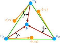
Figure 3: Illustration of the definition of $S$ in the proof of Lemma 3. $v_{1},v_{2},v_{3}$ represent the vertices of the simplex in $\mathbb{R}^{3}$ and $p$ is the fixed point of $\phi$. The vector $\phi(v_{k})$, $k\in[3]$, may not be in the simplex. The linear function $S$ maps vector $(\phi-I)(v_{k})$ into $p-v_{k}$.

To prove Theorem 6, we will use the following lemma (which proves the above characterization in the case of a single transformation $\phi$).

Lemma 3.

Let $\phi:\mathbb{R}^{d}\rightarrow\mathbb{R}^{d}$ be a linear function, and let $\mathcal{P}\subseteq\mathbb{R}^{d}$ be a convex set. Then the following two conditions are equivalent:

• There exists an invertible linear transformation $S$ such that $\phi^{\prime}(p)=p+S(\phi(p)-p)$ is constant for all $p\in\mathcal{P}$.

• $\phi(p)$ has a single fixed point $p_{\phi}$ in $\operatorname*{span}_{\mathsf{Aff}}(\mathcal{P})$.

Proof.

First, assume there does exist such a linear transformation $S$. Assume to the contrary that $\phi$ has two distinct fixed points $p_{1},p_{2}\in\operatorname*{span}_{\mathsf{Aff}}(\mathcal{P})$. Note that $\phi^{\prime}(p_{1})=p_{1}+S(\phi(p_{1})-p_{1})=p_{1}$ so $p_{1}$ is a fixed point of $\phi^{\prime}$; likewise $p_{2}$ is a fixed point of $\phi^{\prime}$. But if $\phi^{\prime}$ is constant on $\mathcal{P}$, it must (as a linear transformation) must also be constant on $\operatorname*{span}_{\mathsf{Aff}}(\mathcal{P})$, implying that we must have $\phi^{\prime}(p_{1})=\phi^{\prime}(p_{2})$, a contradiction.

Now, assume $\phi(p)$ contains a single fixed point $p_{\phi}\in\operatorname*{span}_{\mathsf{Aff}}(\mathcal{P})$. If $\dim(\operatorname*{span}_{\mathsf{Aff}}(\mathcal{P}))=k$, pick any $k$ points $v_{1},v_{2},\dots,v_{k}\in\mathcal{P}$ that together with $p_{\phi}$ affinely span $\mathcal{P}$. In particular, the $k$ vectors $(v_{i}-p_{\phi})$ are linearly independent.

For each $i\in[k]$, let $w_{i}=\phi(v_{i})-v_{i}$. We claim that the $k$ vectors $w_{i}$ are also linearly independent. If they were not, there would exist a non-trivial linear combination $\sum_{i}\lambda_{i}w_{i}$ equal to $0$. Expanding this out (and using the fact that $\phi$ is linear), we have

$$\phi\left(\sum_{i}\lambda_{i}v_{i}\right)=\sum_{i}\lambda_{i}v_{i}.$$

Let $L=\sum_{i}\lambda_{i}$. Adding $(1-L)p_{\phi}$ to both sides (and using the fact that $\phi(p_{\phi})=p_{\phi}$) we have

$$\phi\left((1-L)p_{\phi}+\sum_{i}\lambda_{i}v_{i}\right)=(1-L)p_{\phi}+\sum_{i}\lambda_{i}v_{i}.$$

But the element $v=(1-L)p_{\phi}+\sum_{i}\lambda_{i}v_{i}$ belongs to $\operatorname*{span}_{\mathsf{Aff}}(\mathcal{P})$, so (by assumption) the only way it could be a fixed point of $\phi$ is if $v=p_{\phi}$. But $v-p_{\phi}=\sum_{i}\lambda_{i}(v_{i}-p)$, so this would imply that the original vectors $p-v_{i}$ were not linearly independent, a contradiction.

We can now directly construct our transformation $S$. We will choose any invertible $S$ that satisfies

$$S(\phi(v_{i})-v_{i})=p_{\phi}-v_{i}$$

for all $i\in[k]$. Since both sets of vectors $w_{i}=\phi(v_{i})-v_{i}$ and $p_{\phi}-v_{i}$ are linearly independent, we can choose an invertible such $S$ (technically we also need to specify the action of $S$ on vectors not contained in the span of $w_{i}$, but for these we can choose an arbitary invertible transformation between the remaining sets of basis vectors).

We now claim that the resulting $\phi^{\prime}(p)=p+S(\phi(p)-p)$ is a constant function (and in fact, equals $p_{\phi}$ for all $p\in\mathcal{P}$). To see this, write any $p$ in the form $p=p_{\phi}+\sum_{i=1}^{k}\lambda_{i}(v_{i}-p_{\phi})$ for some $\lambda_{i}\in\mathbb{R}$. Then

$$S(\phi(p)-p)=\sum_{i=1}^{k}\lambda_{i}S(\phi(v_{i})-v_{i})=\sum_{i=1}^{k}\lambda_{i}(p_{\phi}-v_{i})=-\sum_{i=1}^{k}\lambda_{i}(v_{i}-p_{\phi}),$$

and therefore $p+S(\phi(p)-p)=p_{\phi}$, as desired. ∎

We can now complete the proof of Theorem 6.

Proof of Theorem 6.

We first prove that both conditions are necessary. The necessity of the first condition follows immediately from Lemma 3. To see that the second condition is necessary, consider any $\phi_{1},\phi_{2}\in\Phi$. By (17) we have

$$\phi^{\prime}_{1}(p) =p+S(\phi_{1}(p)-p)$$

$$\phi^{\prime}_{2}(p) =p+S(\phi_{2}(p)-p)$$

and therefore

$$\phi^{\prime}_{1}(p)-\phi^{\prime}_{2}(p)=S(\phi_{1}(p)-\phi_{2}(p)).$$

If $S$ is invertible and $\phi^{\prime}_{1}(p)-\phi^{\prime}_{2}(p)$ is a constant for all $p\in\mathcal{P}$, then $\phi_{1}(p)-\phi_{2}(p)$ must also be a constant for all $p\in\mathcal{P}$.

To show that these two conditions are sufficient, single out a representative $\psi\in\Phi$. By Lemma 3 we can construct an $S$ such that the corresponding $\psi^{\prime}$ satisfies

$$\psi^{\prime}(p)=p+S(\psi(p)-p)=p_{\psi}$$

for all $p\in\mathcal{P}$. Now, since any pair of functions in $\Phi$ differ by a constant, for each $\phi\in\Phi$, write $\phi(p)=\psi(p)+\delta_{\phi}$ where $\delta_{\psi}$ is some $p$-independent constant in $\mathbb{R}^{d}$. If we let $p_{\phi}$ denote the fixed point of $\phi$ in $\mathcal{P}$, then since $\phi(p_{\phi})=p_{\phi}$, so we can deduce that $\delta_{\phi}=p_{\phi}-\psi(p_{\phi})$. Note then that

$$\phi^{\prime}(p) = p+S(\phi(p)-p)$$

$$= p+S(\psi(p)+\delta_{\phi}-p)$$

$$= p+S(\psi(p)-p+p_{\phi}-\psi(p_{\phi}))$$

$$= p+(p_{\psi}-p)-(p_{\psi}-p_{\phi})$$

$$= p_{\phi},$$

so each $\phi^{\prime}(p)$ is constant for all $p\in\mathcal{P}$. ∎

4.4 Reducing improper $\phi$-regret to proper $\phi$-regret

Theorem 6 shows that the property of being equivalent to an external regret minimization problem is rather stringent: only very structured improper $\phi$-regret minimization problems (and hence, approachability instances) can be reduced via linear transformations to such instances.

However, the class of proper $\phi$-regret minimization problems is far broader than the class of external regret minimization problems. Notably, every regret minimization problem we have considered thus far either is or is linearly equivalent to a proper $\phi$-regret minimization instance. This raises the natural question of whether every improper $\phi$-regret minimization instance can be linearly transformed into a proper one.

In this section we show that the answer to this question is no. In Section 4.4.1 we give some examples of “atypical” improper $\phi$-regret minimization problems that we prove are not linearly equivalent to any proper $\phi$-regret minimization problems.

Given this, we can also ask whether (in the same vein as Theorem 6) we can cleanly characterize the set of regret-minimization problems which are equivalent to proper $\phi$-regret minimization. In Section 4.4.2 we give an algorithmic procedure for deciding whether a given regret-minimization instance can be reduced to a proper one in the case where the sets $\mathcal{P}$, $\mathcal{L}$, and $\Phi$ are all polytopes.

4.4.1 Irreducible improper instances

In this section we provide two (classes of) examples of improper $\phi$-regret minimization problems that cannot be linearly reduced to a proper $\phi$-regret minimization problem. These two examples will each illustrate different obstructions to the property of being reducible.

Throughout this section, we will assume that $\mathcal{P}=\Delta_{d}$ and $\mathcal{L}=[0,1]^{d}$, and only vary the set $\Phi$. Before we introduce our first class of examples, we will prove the following lemma, which shows that if the instance $\mathcal{I}=(\mathcal{P},\mathcal{L},\Phi)$ is linearly equivalent to a proper $\phi$-regret minimization problem, then all transformations in $\Phi$ must share a left eigenvector of eigenvalue $1$.

Lemma 4.

Assume $\mathcal{P}$ is contained within an affine subspace of $\mathbb{R}^{d}$. If $(\mathcal{P},\mathcal{L},\Phi)$ is linearly equivalent to an instance of proper $\phi$-regret minimization, then there exists a non-zero $v\in\mathbb{R}^{d}$ such that $\langle\phi(p),v\rangle=\langle p,v\rangle$ for any $\phi\in\Phi$ and $p\in\mathcal{P}$.

Proof.

By (17), this linear equivalence sends $\phi(p)$ to the function $\phi^{\prime}(p)=p+S(\phi(p)-p)$, for some invertible linear transformation $S$. Since the target regret minimization instance is proper, $\phi^{\prime}(p)$ is guaranteed to lie in $\mathcal{P}$.

Now, since $\mathcal{P}$ is contained within an affine subspace of $\mathbb{R}^{d}$, there exists some $w\in\mathbb{R}^{d}$ and $b\in\mathbb{R}$ such that $\langle p,w\rangle=b$ for all $p\in\mathcal{P}$. This implies that

$$\langle\phi^{\prime}(p),w\rangle=\langle p,w\rangle+\langle S(\phi(p)-p),w\rangle.$$

Since $\langle\phi^{\prime}(p),w\rangle=\langle p,w\rangle=b$, this reduces to $\langle S(\phi(p)-p),w\rangle=0$, which in turn can be written as $\langle\phi(p)-p,S^{T}w\rangle=0$. Therefore the vector $S^{T}w$ satisfies the constraints for $v$ in the lemma statement. ∎

Note that since the simplex $\Delta_{d}$ is contained within the affine hyperplane $\sum_{i}p_{i}=1$, Lemma 4 applies for all examples in this section. Also, we can alternatively think of the statement of Lemma 4 as stating that the matrices $M_{\phi}$ must all share a non-trivial left kernel element (an element $v$ such that $v^{T}M_{\phi}=0$). To construct an irreducible instance, it suffices to find examples of convex sets of matrices that do not all share the same left kernel element.

Constructing such a set is made more difficult by the fact that each $\phi\in\Phi$ must have a fixed point in $\mathcal{P}$, which translates to the fact that every matrix $M_{\phi}$ must have a non-trivial right kernel element $p_{\phi}$ whose entries are all non-negative (any such element can be scaled to lie in $\mathcal{P}=\Delta_{d}$). We would also like the different $M_{\phi}$ to not all share the same right kernel element (because in that case each $\phi\in\Phi$ would have the same fixed point, and the instance would not be minimal).

We can construct such a set by noticing that the set of skew-symmetric matrices of odd dimension is a linear subspace of the set of matrices. In particular, if for some $a,b,c\in\mathbb{R}_{\geq 0}$ we consider the skew-symmetric matrix

$$M_{\phi_{a,b,c}}=\begin{pmatrix}0&a&-b\\ -a&0&c\\ b&-c&0\end{pmatrix},$$

then the vector $v=(c,b,a)$ belongs to both the left-kernel and right-kernel of $M_{\phi_{a,b,c}}$. In particular, this means that if we take $\Phi=\operatorname*{conv}(\phi_{1,0,0},\phi_{0,1,0},\phi_{0,0,1})$ where:

$$\phi_{1,0,0}(p_{1},p_{2},p_{3}) =(p_{1}-p_{2},\,p_{1}+p_{2},\,p_{3})$$

$$\phi_{0,1,0}(p_{1},p_{2},p_{3}) =(p_{1}+p_{3},\,p_{2},\,p_{3}-p_{1})$$

$$\phi_{0,0,1}(p_{1},p_{2},p_{3}) =(p_{1},\,p_{2}-p_{3},\,p_{2}+p_{3}),$$

then $\mathcal{I}=(\mathcal{P},\mathcal{L},\Phi)$ is a valid improper $\phi$-regret minimization instance which, by Lemma 4, is not linearly equivalent to a proper $\phi$-regret minimization instance.

One might wonder whether Lemma 4 is the sole obstacle to linear equivalence to proper $\phi$-regret minimization. Interestingly, this is not the case. We now give a second $\Phi$ that does not violate Lemma 4 (i.e., all $M_{\phi}$ share a left-kernel element), but where the instance $(\mathcal{P},\mathcal{L},\Phi)$ is still provably not linearly equivalent to proper $\phi$-regret minimization. To do so, we will rely on the following obstruction.

Lemma 5.

Consider an improper $\phi$-regret minimization instance $\mathcal{I}=(\mathcal{P},\mathcal{L},\Phi)$. If there exists an extreme point $x$ of $\mathcal{P}$ and $\phi_{1},\phi_{2}\in\Phi$ with the property that

$$\phi_{2}(x)-x=-\alpha(\phi_{1}(x)-x)\neq 0$$

for some real $\alpha>0$, then $\mathcal{I}$ is not linearly equivalent to a proper $\phi$-regret minimization instance.

Proof.

If such a linear equivalence existed, by (17), we would have that $\phi^{\prime}_{1}(x)=x+S(\phi_{1}(x)-x)$ and $\phi^{\prime}_{2}(x)=x+S(\phi_{2}(x)-x)=x-\alpha S(\phi_{1}(x)-x)$. But since $x$ is an extreme point of $\mathcal{P}$, it is impossible for both $x+w$ and $x-\alpha w$ to both lie in $\mathcal{P}$ for a non-zero vector $w$. ∎

We now present a valid improper $\phi$-regret minimization instance (found by computer search) where Lemma 5 applies but Lemma 4 does not. This example is parametrized by the two matrices:

$$A=\begin{pmatrix}-6&8&-9\\ 2&-1&-9\\ 4&-7&18\end{pmatrix},B=\begin{pmatrix}10&-3&-7\\ 6&-6&10\\ -16&9&-3\end{pmatrix}.$$

Note that both $A$ and $B$ share the same left-kernel element $(1,1,1)$ (so they both map the hyperplane containing $\mathcal{P}$ to itself). We will consider the set of regret functions $\Phi=\{\operatorname{Id}+\gamma_{a}A+\gamma_{b}B\mid\gamma_{a}\in[-1,1],\gamma_{b}\in[-1,1]\}$. One can also verify computationally that all elements of $\Phi$ contain a fixed point within the simplex $\Delta_{3}$ and that this fixed point is not static and changes depending on $\gamma_{b}/\gamma_{a}$ (see Figure 4).

Figure 4: For any $t$, the matrix $M(t)=A+tB$ has a right kernel element of the form $(x(t),y(t),1)$, where $x(t)=\frac{72t^{2}-46t+81}{2(21t^{2}+8t+5)}$ and $y(t)=\frac{72t^{2}-41t+36}{21t^{2}+8t+5}$. The above diagram plots $(x(t),y(t))$ for all $t\in\mathbb{R}$, and shows that this right kernel element always has non-negative entries (and hence has a multiple that lies in $\Delta_{3}$).

But now, consider the two functions $\phi_{1}(p)=p+Ap$ and $\phi_{2}(p)=p-Ap$ both belonging to $\Phi$. For any $x\in\mathcal{P}$ it is the case that $\phi_{1}(x)-x=Ax=-(\phi_{2}(x)-x)$. Choosing $x$ to b e the extreme point $(1,0,0)$, $Ax$ is non-zero and thus by Lemma 4 this instance is not equivalent to a proper $\phi$-regret minimization instance.

4.4.2 An algorithmic characterization

Finally, we will show how to algorithmically decide whether a given regret minimization instance $\mathcal{I}=(\mathcal{P},\mathcal{L},\mathcal{I})$ is linearly equivalent to a proper $\phi$-regret minimization problem via solving an appropriate linear program for the transformation $S$. For simplicity, we will only handle the case where $\mathcal{P}$ and $\mathcal{I}$ are both polytopes, with $\mathcal{P}$ being the convex hull of the $N$ vertices $p_{1},p_{2},\dots,p_{N}$ and $\mathcal{I}$ being the convex hull of the $M$ regret functions $\phi_{1},\phi_{2},\dots,\phi_{M}$.

Recall that (by (17)) we have $\phi^{\prime}_{i}(p)=p+S(\phi(p)-p)$. Note that $\phi^{\prime}$ is a proper $\phi$-function if and only if $\phi^{\prime}_{i}(p_{j})$ lies within $\mathcal{P}$ for all vertices $p_{j}$ (by convexity, this implies that $\phi^{\prime}_{i}(p)\in\mathcal{P}$ for any other $p\in\mathcal{P}$). So there exists a reduction iff there exists an invertible $S$ such that for every $i\in[M]$ and $j\in[N]$, we have the constraint

$$p_{j}+S(\phi_{i}(p_{j})-p_{j})\in\mathcal{P}.$$ (18)

We can in turn rephrase (18) as several linear constraints on the entries of the matrix $S$. In particular, if we introduce the auxiliary variables $\lambda_{i,j,k}$ (for $k\in[N]$) we can rewrite the set of constraints expressed by (18) as the following linear program (whose variables are the $d^{2}$ entries of $S$ and the $\lambda_{i,j,k}$):

$$p_{j}+S(\phi_{i}(p_{j})-p_{j}) = \sum_{k=1}^{N}\lambda_{i,j,k}p_{k}\text{ for all }i\in[M],j\in[N]$$

$$\sum_{k=1}^{N}\lambda_{i,j,k} = 1\text{ for all }i\in[M],j\in[N]$$

$$\lambda_{i,j,k} \geq 0\text{ for all }i\in[M],j,k\in[N]$$

The above constraints define a convex cone of possible values of $S$ which we denote by $\mathcal{S}$. For example, this cone always contains the solution $S=0$; we would like to now decide whether it contains any invertible matrices. Luckily, this is straightforward to do in a randomized manner by the following lemma.

Lemma 6.

Given any convex set $\mathcal{S}\subseteq\mathbb{R}^{d\times d}$ of $d$-by-$d$ matrices, either every matrix in $\operatorname*{span}(\mathcal{S})$ is non-invertible, or almost all matrices in $\operatorname*{span}(\mathcal{S})$ are invertible.

Proof.

Given any linear subspace of matrices $V\subseteq\mathbb{R}^{d\times d}$, the constraint $\det(M)=0$ defines an algebraic variety on this space. Any algebraic variety in a Euclidean space either has measure zero or is equal to the entire space. ∎

Given this, it suffices to simply test whether a random element in $\operatorname*{span}(\mathcal{S})$ is invertible. We can efficiently generate a basis of $\operatorname*{span}(\mathcal{S})$ by repeatedly solving the linear program above (finding the extreme points in $\mathcal{S}$ in a direction orthogonal to all basis elements found so far), and once we have such a basis, we can test a random linear combination of the basis elements for invertibility.

This entire procedure takes time polynomial in $N$, $M$, and $d$. It can also likely be extended beyond polytopes to any case where have a membership oracle for $\mathcal{S}$ (i.e., a procedure that decides whether (18) is satisfied for all $\phi\in\Phi$ and $p\in\mathcal{P}$), modulo numerical issues with testing invertibility. Note also that this procedure not only checks whether a given instance is reducible, by also provides a valid transformation $S$ in the case that it is.

5 Conclusion

This work uncovers a nuanced relationship between Blackwell’s approachability and no-regret learning. While fundamentally equivalent, this equivalence does not always preserve optimal convergence rates, highlighting the importance of understanding the fine-grained details of reductions between these problems. Our introduction of improper $\phi$-regret minimization provides a useful tool for bridging this gap, allowing for tight reductions from any approachability instance to a generalized regret minimization problem. The existence of improper $\phi$-regret instances that cannot be reduced to standard classes suggests that approachability covers a broader range of problems than can be easily expressed in traditional online learning terms. This also motivates a more detailed study of the complex relationship between approachability and improper $\phi$-regret, potentially leading to deeper connections and new algorithmic solutions.

Appendix A Approaching the negative orthant

In this appendix we show that any approachability problem can equivalently be written in terms of approaching the negative orthant.

Traditionally (as in Blackwell [1956]), instead of specifying a constraint set $\mathcal{U}$, an approachability problem specifies a vector-valued bilinear payoff function ${\mathbf{u}}\colon\mathcal{P}\times\mathcal{L}\rightarrow\mathbb{R}^{k}$ along with a set $\mathcal{S}\subseteq\mathbb{R}^{k}$ that the learner would like to approach. In particular, they would like to minimize the average distance

$$\operatorname{\mathsf{AppDist}}({\mathbf{p}},{\bm{\ell}})=\mathrm{dist}_{\nu}\left(\frac{1}{T}\sum_{t=1}^{T}{\mathbf{u}}(p_{t},\ell_{t}),\mathcal{S}\right),$$

where $\mathrm{dist}(x,\mathcal{S})$ is the minimum distance between $x$ and the set $\mathcal{S}$ under some norm $\nu$. We prove the following result:

Theorem 7.

For any norm $\nu$, set $\mathcal{S}$, and payoff ${\mathbf{u}}$, there exists a corresponding convex set $\mathcal{U}\subseteq\mathsf{Aff}(\mathcal{P}\otimes\mathcal{L},\mathbb{R})$ such that

$$\operatorname{\mathsf{AppDist}}({\mathbf{p}},{\bm{\ell}})=\operatorname{\mathsf{AppLoss}}({\mathbf{p}},{\bm{\ell}}).$$

where here $\operatorname{\mathsf{AppLoss}}$ is understood to mean the approachability loss (1) with respect to the set of constraints $\mathcal{U}$.

Proof.

For any $r$, consider the set of points $\mathcal{S}_{r}$ within distance $r$ (under $\nu$) of $\mathcal{S}$. We can write $\mathcal{S}_{r}$ as $\mathcal{S}+rB$, where $B$ is the unit ball in the norm $\nu$. We can then write $\mathcal{S}_{r}$ as the intersection of the extremal halfspaces in all directions, where the extremal halfspace in direction $v$ (for any $v\in\mathbb{S}^{d-1}$ on the unit sphere) can be written in the form:

$$\{x\in\mathbb{R}^{k}\mid\langle v,x\rangle\leq a_{v}+b_{v}r\}$$

for some constants $a_{v}$ and $b_{v}$ (with $b_{v}\geq 0$). It follows that for any $x\in\mathbb{R}^{k}$, we can write

$$\mathrm{dist}_{\nu}(x,\mathcal{S})=\max_{v\in\mathbb{S}^{d-1}}\left(\frac{\langle v,x\rangle-a_{v}}{b_{v}}\right).$$

If we choose our set $\mathcal{U}$ to contain all functions $u_{v}$ of the form

$$u_{v}(p,\ell)=\frac{\langle v,{\mathbf{u}}(p,\ell)\rangle-a_{v}}{b_{v}},$$

(for all $v\in\mathbb{S}^{d-1}$), then it follows that $\operatorname{\mathsf{AppDist}}({\mathbf{p}},{\bm{\ell}})=\operatorname{\mathsf{AppLoss}}({\mathbf{p}},{\bm{\ell}})$. ∎

Appendix B Non-degenerate counterexample to the reduction

One may object that the approachability instance $\mathcal{I}$ presented in Theorem 3 with $\operatorname{\mathsf{Rate}}(\mathcal{I})=0$ is somewhat degenerate, as there is a single action by the learner that perfectly approaches the negative orthant. In this appendix we show that this is easily addressed; we can use a similar construction to obtain non-degenerate approachability instances where $\operatorname{\mathsf{Rate}}(\mathcal{I}^{\prime})/\operatorname{\mathsf{Rate}}(\mathcal{I})$ is arbitrarily large. The main idea is to embed a non-trivial (but very easy) regret-minimization problem on the “unused” coordinates of the instance.

Theorem 8.

For any $c>0$, we can construct an approachability instance $\mathcal{I}$ such that $\operatorname{\mathsf{Rate}}(\mathcal{I}^{\prime})>c\cdot\operatorname{\mathsf{Rate}}(\mathcal{I})$, where $\mathcal{I}^{\prime}$ is the regret minimization instance obtained by applying the reduction of Theorem 2 to $\mathcal{I}$. In particular, there is no finite $c>0$ for which the reduction in Theorem 2 is a $c$-approximate reduction for all approachability instances, and the reduction is not tight.

Proof.

Consider the following approachability instance $\mathcal{I}$. Fix any $\varepsilon>0$, $d_{1},d_{2}>1$ and let $d=d_{1}+d_{2}$. We will let $\mathcal{P}=\Delta_{d}$, $\mathcal{L}=[0,1]^{d}$, and $\mathcal{U}$ to be the convex hull of the $d$ bilinear functions $u_{i}$, where for $i\in[d_{1}]$,

$$u_{i}(p,\ell)=\varepsilon\sum_{j=1}^{d_{1}}p_{j}(\ell_{j}-\ell_{i}),$$

and for $i\in[d_{2}]$,

$$u_{d_{1}+i}(p,\ell)=\sum_{j=d_{1}+1}^{d_{1}+d_{2}}p_{j}(\ell_{j}-\ell_{d_{1}+i}).$$

Here the $u_{i}$ constraint for $i\in[d_{1}]$ can be thought of as the regret of moving all probability mass on $p_{1}$ through $p_{d_{1}}$ to $p_{i}$ (but weighted by $\varepsilon$); similarly, the $u_{d_{1}+i}$ constraint can be thought of as the regret of moving all probability mass on $p_{d_{1}+1}$ through $p_{d}$ to $p_{d_{1}+i}$.

We will first show that $\operatorname{\mathsf{Rate}}(\mathcal{I})=O(\varepsilon\sqrt{\log d_{1}})$. To see this, note that if we ignore the last $d_{2}$ coordinates (always assigning weight $0$ to them) and run a standard online-learning algorithm over the simplex $\Delta_{d_{1}}$ (e.g., Hedge) it is possible to construct an approachability algorithm $\mathcal{A}$ with $\operatorname{\mathsf{AppLoss}}_{T}(\mathcal{A})=O(\sqrt{T\log d_{1}})$.

However, the instance of external regret minimization we reduce to will have a worse rate. Let $\mathcal{I}^{\prime}=(\mathcal{P}^{\prime},\mathcal{L}^{\prime},\Phi^{\prime})$ be the regret minimization instance formed by applying the reduction of Theorem 2. This instance has $\mathcal{P}^{\prime}=\mathcal{U}$, $\mathcal{L}^{\prime}=-(\mathcal{P}\otimes\mathcal{L})$, and $\mathcal{U}^{\prime}$ the set of all constant functions on $\mathcal{P}^{\prime}$. We will restrict the loss set further, and insist that the only losses $\ell^{\prime}_{t}$ are of the form $\ell^{\prime}_{t}=-(U_{d_{2}}\otimes\ell_{t})$, where $U_{d_{2}}=(0,0,\dots,0,1/d_{2},1/d_{2},\dots,1/d_{2})\in\mathcal{P}$ is the uniform distribution over the last $d_{2}$ coordinates, and $\ell_{t}$ is chosen from the subset $\mathcal{L}_{2}\subseteq\mathcal{L}$ contains all elements of $\mathcal{L}$ whose first $d_{1}$ coordinates equal $0$ (so $\mathcal{L}_{2}\cong[0,1]^{d_{2}}$). Since this restricts the adversary, it only makes the regret minimization problem easier (and the rate smaller).

The regret of a pair of sequences ${\mathbf{p}}^{\prime}$ and ${\bm{\ell}}^{\prime}$ for this new problem can be written as

$$\operatorname{\mathsf{Reg}}({\mathbf{p}}^{\prime},{\bm{\ell}}^{\prime})=\max_{x^{*}\in\mathcal{P}^{\prime}}\left(\sum_{t=1}^{T}\langle p^{\prime}_{t},\ell^{\prime}_{t}\rangle-\sum_{t=1}^{T}\langle x^{*},\ell^{\prime}_{t}\rangle\right).$$ (19)

To simplify this further, note that the set $\mathcal{P}^{\prime}=\mathcal{U}$ is given by the convex hull of the $d$ bilinear functions $u_{i}$, so we can write each element of $\mathcal{P}^{\prime}$ uniquely as a convex combination of this $d$ functions. For a $p^{\prime}_{t}\in\mathcal{P}^{\prime}$, we will write $p^{\prime}_{i}$ to be the coefficient of $u_{i}$ in this convex combination (in this way, we identify $\mathcal{P}^{\prime}$ with the simplex $\Delta_{d}$).

Now, for any $p^{\prime}\in\mathcal{P}^{\prime}$ and $\ell^{\prime}\in\mathcal{L}^{\prime}$ (of the above restricted form), we can write

$$\langle p^{\prime},\ell^{\prime}\rangle=-\sum_{i=d_{1}+1}^{d_{1}+d_{2}}p^{\prime}_{i}\left(\frac{1}{d_{2}}\sum_{j=d_{1}+1}^{d_{1}+d_{2}}(\ell_{j}-\ell_{i})\right)=\left\langle\pi_{2}(p^{\prime}),\pi_{2}(\ell)\right\rangle-\frac{1}{d_{2}}\left(\sum_{i=1}^{d_{2}}\pi_{2}(p^{\prime})_{i}\right)\left(\sum_{i=1}^{d_{2}}\pi_{2}(\ell)_{i}\right),$$ (20)

where $\pi_{2}:\mathbb{R}^{d}\rightarrow\mathbb{R}^{d_{2}}$ is the projection map onto the last $d_{2}$ coordinates. We can simplify this even further by introducing the map $\overline{\pi}:\Delta_{d}\rightarrow\Delta_{d_{2}}$ defined via

$$\overline{\pi}(p^{\prime})_{i}=p^{\prime}_{d_{1}+i}+\frac{1}{d_{2}}\left(1-\sum_{j=1}^{d_{2}}p^{\prime}_{d_{1}+j}\right).$$ (21)

This allows us to rewrite (20) as

$$\langle p^{\prime},\ell^{\prime}\rangle=\langle\overline{\pi}(p^{\prime}),\pi_{2}(\ell)\rangle-\sum_{j=d_{1}+1}^{d_{2}}\ell_{j}.$$ (22)

Substituting this in turn into (19), we have that

$$\operatorname{\mathsf{Reg}}({\mathbf{p}}^{\prime},{\bm{\ell}}^{\prime})=\max_{x^{*}\in\mathcal{P}^{\prime}}\left(\sum_{t=1}^{T}\langle\overline{\pi}(p^{\prime}_{t}),\pi_{2}(\ell_{t})\rangle-\sum_{t=1}^{T}\left\langle\overline{\pi}(x^{*}),\pi_{2}(\ell_{t})\right\rangle\right).$$ (23)

Now, note that the adversary can choose $\ell_{t}$ so that $\pi_{2}(\ell_{t})$ takes on any value in $\mathcal{L}_{2}=[0,1]^{d_{2}}$. Similarly, $\overline{\pi}(p^{\prime})$ can take on any value in $\mathcal{P}_{2}=\Delta_{d_{2}}$ as $p^{\prime}$ ranges over $\mathcal{P}^{\prime}$. Therefore, this problem is at least as hard as the online linear optimization problem with action set $\mathcal{P}_{2}=\Delta_{d_{2}}$ and loss set $\mathcal{L}_{2}=[0,1]^{d_{2}}$. But this is exactly the online learning with experts problem (with $d_{2}$ experts), which has a regret lower bound of $\Omega(\sqrt{T\log d_{2}})$. It follows that $\operatorname{\mathsf{Rate}}(\mathcal{I}^{\prime})\geq\Omega(\sqrt{\log d_{2}})$, and therefore that $\operatorname{\mathsf{Rate}}(\mathcal{I}^{\prime})/\operatorname{\mathsf{Rate}}(\mathcal{I})>\Omega(\sqrt{(\log d_{2})/(\log d_{1})}/\varepsilon)$. This quantity can be made arbitrarily large (for a fixed $d_{1}$ and $d_{2}$) as we decrease $\varepsilon$. ∎

References

- Abernethy et al. [2011] J. D. Abernethy, P. L. Bartlett, and E. Hazan. Blackwell approachability and no-regret learning are equivalent. In Proceedings of COLT, volume 19 of JMLR Proceedings, pages 27–46, 2011.
- Agrawal et al. [2018] S. Agrawal, C. Daskalakis, V. S. Mirrokni, and B. Sivan. Robust repeated auctions under heterogeneous buyer behavior. In É. Tardos, E. Elkind, and R. Vohra, editors, Proceedings of the 2018 ACM Conference on Economics and Computation, Ithaca, NY, USA, June 18-22, 2018, page 171. ACM, 2018.
- Bai et al. [2022] Y. Bai, C. Jin, S. Mei, Z. Song, and T. Yu. Efficient phi-regret minimization in extensive-form games via online mirror descent. Advances in Neural Information Processing Systems, 35:22313–22325, 2022.
- Blackwell [1956] D. Blackwell. An analog of the minimax theorem for vector payoffs. Pacific Journal of Mathematics, 6(1):1–8, 1956.
- Blum and Mansour [2007] A. Blum and Y. Mansour. From external to internal regret. Journal of Machine Learning Research, 8:1307–1324, 2007.
- Braverman et al. [2018] M. Braverman, J. Mao, J. Schneider, and S. M. Weinberg. Selling to a no-regret buyer. In É. Tardos, E. Elkind, and R. Vohra, editors, Proceedings of the 2018 ACM Conference on Economics and Computation, Ithaca, NY, USA, June 18-22, 2018, pages 523–538. ACM, 2018.
- Cai et al. [2023] L. Cai, S. M. Weinberg, E. Wildenhain, and S. Zhang. Selling to multiple no-regret buyers. In J. Garg, M. Klimm, and Y. Kong, editors, Web and Internet Economics - 19th International Conference, WINE 2023, Shanghai, China, December 4-8, 2023, Proceedings, volume 14413 of Lecture Notes in Computer Science, pages 113–129. Springer, 2023.
- Celli et al. [2021] A. Celli, A. Marchesi, G. Farina, N. Gatti, et al. Decentralized no-regret learning algorithms for extensive-form correlated equilibria. In IJCAI, pages 4755–4759, 2021.
- Chzhen et al. [2021] E. Chzhen, C. Giraud, and G. Stoltz. A unified approach to fair online learning via blackwell approachability. In Proceedings of NeurIPS, pages 18280–18292, 2021.
- Dagan et al. [2023] Y. Dagan, C. Daskalakis, M. Fishelson, and N. Golowich. From external to swap regret 2.0: An efficient reduction and oblivious adversary for large action spaces. arXiv preprint arXiv:2310.19786, 2023.
- Dann et al. [2023] C. Dann, Y. Mansour, M. Mohri, J. Schneider, and B. Sivan. Pseudonorm approachability and applications to regret minimization. In S. Agrawal and F. Orabona, editors, International Conference on Algorithmic Learning Theory, February 20-23, 2023, Singapore, volume 201 of Proceedings of Machine Learning Research, pages 471–509. PMLR, 2023.
- Dawid [1982] A. P. Dawid. The well-calibrated bayesian. Journal of the American Statistical Association, 77(379):605–610, 1982. doi: 10.1080/01621459.1982.10477856. URL https://www.tandfonline.com/doi/abs/10.1080/01621459.1982.10477856.
- Deng et al. [2019] Y. Deng, J. Schneider, and B. Sivan. Strategizing against no-regret learners. In Advances in Neural Information Processing Systems 32: Annual Conference on Neural Information Processing Systems 2019, NeurIPS 2019, 8-14 December 2019, Vancouver, BC, Canada, pages 1577–1585, 2019. URL http://papers.nips.cc/paper/8436-strategizing-against-no-regret-learners.
- Foster and Hart [2018] D. P. Foster and S. Hart. Smooth calibration, leaky forecasts, finite recall, and nash dynamics. Games and Economic Behavior, 109:271–293, 2018. ISSN 0899-8256. doi: https://doi.org/10.1016/j.geb.2017.12.022. URL https://www.sciencedirect.com/science/article/pii/S0899825618300113.
- Foster and Vohra [1997] D. P. Foster and R. V. Vohra. Calibrated learning and correlated equilibrium. Games and Economic Behavior, 21(1-2):40–55, 1997.
- Foster and Vohra [1999] D. P. Foster and R. V. Vohra. Regret in the on-line decision problem. Games and Economic Behavior, 29(1-2):7–35, 1999.
- Gordon et al. [2008] G. J. Gordon, A. Greenwald, and C. Marks. No-regret learning in convex games. In Proceedings of ICML, volume 307, pages 360–367. ACM, 2008.
- Greenwald and Jafari [2003] A. Greenwald and A. Jafari. A general class of no-regret learning algorithms and game-theoretic equilibria. In Proceedings of COLT, volume 2777 of Lecture Notes in Computer Science, pages 2–12. Springer, 2003.
- Greenwald et al. [2008] A. Greenwald, Z. Li, and W. Schudy. More efficient internal-regret-minimizing algorithms. In COLT, pages 239–250, 2008.
- Hart and Mas-Colell [2000] S. Hart and A. Mas-Colell. A simple adaptive procedure leading to correlated equilibrium. Econometrica, 68(5):1127–1150, 2000.
- Kalathil et al. [2014] D. M. Kalathil, V. S. Borkar, and R. Jain. Blackwell’s approachability in Stackelberg stochastic games: A learning version. In Proceedings of CDC, pages 4467–4472. IEEE, 2014.
- Kwon [2021] J. Kwon. Refined approachability algorithms and application to regret minimization with global costs. The Journal of Machine Learning Research, 22:200–1, 2021.
- Kwon and Perchet [2017] J. Kwon and V. Perchet. Online learning and blackwell approachability with partial monitoring: Optimal convergence rates. In A. Singh and X. J. Zhu, editors, Proceedings of AISTATS, volume 54, pages 604–613. PMLR, 2017.
- Lehrer [2003] E. Lehrer. Approachability in infinite dimensional spaces. Int. J. Game Theory, 31(2):253–268, 2003.
- Mannor and Shimkin [2003] S. Mannor and N. Shimkin. The empirical bayes envelope and regret minimization in competitive markov decision processes. Math. Oper. Res., 28(2):327–345, 2003.
- Mannor et al. [2014a] S. Mannor, V. Perchet, and G. Stoltz. Set-valued approachability and online learning with partial monitoring. J. Mach. Learn. Res., 15(1):3247–3295, 2014a.
- Mannor et al. [2014b] S. Mannor, V. Perchet, and G. Stoltz. Approachability in unknown games: Online learning meets multi-objective optimization. In Proceedings of COLT, volume 35, pages 339–355, 2014b.
- Mansour et al. [2022] Y. Mansour, M. Mohri, J. Schneider, and B. Sivan. Strategizing against learners in bayesian games. In P. Loh and M. Raginsky, editors, Conference on Learning Theory, 2-5 July 2022, London, UK, volume 178 of Proceedings of Machine Learning Research, pages 5221–5252. PMLR, 2022.
- Miryoosefi et al. [2019] S. Miryoosefi, K. Brantley, H. D. III, M. Dudík, and R. E. Schapire. Reinforcement learning with convex constraints. In Proceedings of NIPS, pages 14070–14079, 2019.
- Mohri and Yang [2014] M. Mohri and S. Yang. Conditional swap regret and conditional correlated equilibrium. In NIPS, pages 1314–1322, 2014.
- Mohri and Yang [2017] M. Mohri and S. Yang. Online learning with transductive regret. In Proceedings of NIPS, pages 5214–5224, 2017.
- Peng and Rubinstein [2023] B. Peng and A. Rubinstein. Fast swap regret minimization and applications to approximate correlated equilibria. arXiv preprint arXiv:2310.19647, 2023.
- Perchet [2010] V. Perchet. Approchabilité, Calibration et Regret dans les Jeux à Observations Partielles. PhD thesis, Université Pierre et Marie Curie - Paris VI, 2010.
- Perchet [2015] V. Perchet. Exponential weight approachability, applications to calibration and regret minimization. Dynamic Games and Applications, 5(1):136–153, 2015.
- Perchet and Quincampoix [2015] V. Perchet and M. Quincampoix. On a unified framework for approachability with full or partial monitoring. Mathematics of Operations Research, 40(3):596–610, 2015.
- Perchet and Quincampoix [2018] V. Perchet and M. Quincampoix. A differential game on Wasserstein space. Application to weak approachability with partial monitoring. CoRR, abs/1811.04575, 2018.
- Rubinstein and Zhao [2024] A. Rubinstein and J. Zhao. Strategizing against no-regret learners in first-price auctions. CoRR, abs/2402.08637, 2024.
- Shimkin [2016] N. Shimkin. An online convex optimization approach to blackwell’s approachability. The Journal of Machine Learning Research, 17(1):4434–4456, 2016.
- Spinat [2002] X. Spinat. A Necessary and Sufficient Condition for Approachability. Mathematics of Operations Research, 27(1):31–44, 2002.
- Stoltz and Lugosi [2005] G. Stoltz and G. Lugosi. Internal regret in on-line portfolio selection. Machine Learning, 59(1):125–159, 2005.
- Stoltz and Lugosi [2007] G. Stoltz and G. Lugosi. Learning correlated equilibria in games with compact sets of strategies. Games Econ. Behav., 59(1):187–208, 2007.
- Vieille [1992] N. Vieille. Weak approachability. Math. Oper. Res., 17(4):781–791, 1992.
- Zhang et al. [2024] B. H. Zhang, I. Anagnostides, G. Farina, and T. Sandholm. Efficient phi-regret minimization with low-degree swap deviations in extensive-form games. arXiv preprint arXiv:2402.09670, 2024.