Biharmonic Distance of Graphs and its Higher-Order Variants: Theoretical Properties with Applications to Centrality and Clustering

Abstract

Effective resistance is a distance between vertices of a graph that is both theoretically interesting and useful in applications. We study a variant of effective resistance called the biharmonic distance (Lipman et al., 2010). While the effective resistance measures how well-connected two vertices are, we prove several theoretical results supporting the idea that the biharmonic distance measures how important an edge is to the global topology of the graph. Our theoretical results connect the biharmonic distance to well-known measures of connectivity of a graph like its total resistance and sparsity. Based on these results, we introduce two clustering algorithms using the biharmonic distance. Finally, we introduce a further generalization of the biharmonic distance that we call the $k$-harmonic distance. We empirically study the utility of biharmonic and $k$-harmonic distance for edge centrality and graph clustering.

1 Introduction

Many areas of machine learning, such as clustering (Shi & Malik, 2000), semi-supervised learning (Zhu et al., 2003) and graph mining (Chakrabarti & Faloutsos, 2006), require measuring the distance between two vertices in a graph. Simple distance metrics like the shortest-path distance only consider a single path between vertices but do not contain any information about the global topology of the graph. For many tasks, a better choice of a distance metric is one that accounts for all paths connecting a pair of vertices, thereby capturing aspects of the connectivity of the graph. One commonly used distance metric with this property is effective resistance (Kirchhoff, 1847).

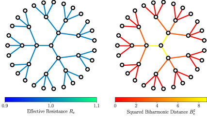
Figure 1: The effective resistance vs. squared biharmonic distance for edges in a tree. While the effective resistance is 1 on all edges, the biharmonic distance is higher on edges closer to the root, demonstrating that biharmonic distance is aware of the global topology of a graph. See Appendix I for more examples.

The effective resistance between vertices $s$ and $t$ in a graph is a distance measure defined

$$R_{st}=(1_{s}-1_{t})^{T}L^{+}(1_{s}-1_{t})$$

where $L^{+}$ is the pseudoinverse of the graph Laplacian and $1_{v}$ is the indicator vector of a vertex $v$.

While effective resistance was originally introduced by Kirchhoff (1847) in the context of electrical networks, it has since been discovered that by treating the mathematics abstractly, effective resistance has many interesting theoretical properties and applications in graph theory. An intuitive explanation of effective resistance is that

Effective resistance measure how well-connected a pair of vertices $s$ and $t$ are.

because the more, and shorter, paths there are connecting $s$ and $t$, the lower the effective resistance between $s$ and $t$. Theoretical works on the effective resistance have reinforced this intuition. For example, it has been shown that effective resistance is proportional to the commute time of random walks between two vertices (Chandra et al., 1996) and is proportional to the probability an edge is in a random spanning tree (Kirchhoff, 1847). Beyond its theoretical appeal, effective resistance is used in various applications, notably in contexts requiring a measure of connectivity, such as clustering (Yen et al., 2005; Khoa & Chawla, 2012; Alev et al., 2018), graph sparsification (Spielman & Srivastava, 2011), edge centrality (Teixeira et al., 2013; Mavroforakis et al., 2015), semi-supervised learning on graphs (Zhu et al., 2003), link prediction (Lü & Zhou, 2011), and as a positional encoding for graph neural networks (Zhang et al., 2023; Velingker et al., 2024).

There are other graph distances similar to effective resistance. For example, the diffusion distance (at time $t$) (Coifman & Lafon, 2006) is $D^{(t)}_{st}=\sqrt{(1_{s}-1_{t})^{T}e^{-tL}(1_{s}-1_{t})}$. Generally, we can consider spectral distances $\sqrt{(1_{s}-1_{t})^{T}f(L)(1_{s}-1_{t})}$ for any function $f$. However, it is an open question which function $f$ defines the best distance for different applications. Unfortunately, besides the effective resistance and diffusion distance, spectral distances are not well-studied and little is known about their theoretical properties or applicability.

Biharmonic distance is one such spectral distance, defined

$$B_{st}=\sqrt{(1_{s}-1_{t})^{T}(L^{+})^{2}(1_{s}-1_{t})}.$$

The biharmonic distance was introduced by Lipman et al. (2010) in the context of geometry processing, where it was noted that the biharmonic distance was seemingly more aware of the global structure of a graph than effective resistance. Subsequent works have begun to use it in other applications, including consensus networks (Yi et al., 2018b, 2021) and as a centrality measure (Li & Zhang, 2018; Yi et al., 2018a). While researchers have begun to study the theoretical properties of the biharmonic distance (Lin, 2022; Wei et al., 2021), biharmonic distance is not nearly as well-understood theoretically as effective resistance.

1.1 Contributions

	Effective Resistance	Biharmonic Distance
Definition	$R_{st}=(1_{s}-1_{t})^{T}L^{+}(1_{s}-1_{t})$	$B_{st}=\sqrt{(1_{s}-1_{t})^{T}L^{2+}(1_{s}-1_{t})}$
Intuitive Explanation	Measures how well-connected the vertices $s$ and $t$ are.	Measures how important the edge $\{s,t\}$ is to the global topology of the graph.
Bounds	$\frac{1}{n}\leq R_{st}\leq n-1$	$\frac{1}{n^{2}}\leq B^{2}_{st}\leq n^{3}$ (Theorems A.1 and A.2)
Bounds on Edges	$R_{e}\leq 1$	$B^{2}_{e}\leq n$ (Theorem A.3)
Sum over Edges	$\sum_{e\in E}w_{e}R_{e}=n-1$	$n\sum_{e\in E}w_{e}B^{2}_{e}=R_{\operatorname{tot}}$ (Corollary 4.3)
Electrical Flows	$R_{st}=\sum_{e\in E}f_{st}^{2}(e)/w_{e}$	$nw_{e}B_{e}^{2}=\sum_{s,t\in V}f_{st}(e)^{2}/w_{e}$ (Theorem 4.1)
Cut Edges	$R_{e}=1$	$B^{2}_{e}=(\text{Cut Sparsity})^{-1}$ (Theorem 5.1)
Edges & Sparsity	-	$B^{2}_{e}\sim(\text{Cut Sparsity})^{-1}$ (Theorems 5.3 and 5.4)

Table 1: A comparison of the effective resistance and biharmonic distance.

We present several new theoretical properties of the biharmonic distance. Our results mainly concern the biharmonic distance of edges in a graph. We propose the following intuitive explanation:

Biharmonic distance measures how important an edge is to the global topology of a graph.

We present several theoretical results that reinforce this intuition. Accordingly, we believe that the biharmonic distance may be a superior choice over other distances like effective resistance for applications where we need to capture the global topology of a graph with respect to the edges.

Electrical Flow and Edge Centrality.

We prove that the biharmonic distance of an edge is proportional to its total usage in electrical flows between all pairs of vertices in the graph (Theorem 4.1). This theorem suggests that edges with high biharmonic distance are important to the connection between many pairs of vertices. This also partially explains the success of biharmonic distance as a measure of centrality. Our theorem also implies a generalization of the well-known Foster’s Theorem to biharmonic distance.

Clustering and Sparse Cuts.

We establish a connection between the biharmonic distance of edges and the sparsity of cuts in the graph. In particular, we prove that sparse cuts necessarily contain edges with high biharmonic values, and conversely, edges with high biharmonic values are contained in sparse cuts. (Theorems 5.3 and 5.4). This result suggests the use of biharmonic distance in graph clustering algorithms, an idea we explore in Section 5.3

Higher-Order Harmonic Distances.

We introduce a generalization of the biharmonic distance called the k-harmonic distance, defined

$$H_{st}^{(k)}=\sqrt{(1_{s}-1_{t})^{T}L^{k+}(1_{s}-1_{t})}.$$

Some of our theoretical results for biharmonic distance generalize to $k$-harmonic distance.

Experiments.

We compare biharmonic and $k$-harmonic distance to other centrality measures in terms of correlation and resilience to change. We also compare our clustering algorithms with other clustering algorithms. We conducted experiments on both synthetic and real world data and observed that algorithms using biharmonic distance consistently outperform effective resistance methods. Furthermore, we observed that $k$-harmonic clustering algorithms achieve optimal results at larger values of $k$.

1.2 Related work

Biharmonic Distance.

Previous works have also hinted at our proposed interpretation of biharmonic distance. These works establish a connection between the total resistance $R_{\operatorname{tot}}$ (aka the Kirchhoff index) of a graph and the biharmonic distance of an edge. The total resistance of a graph is the sum of effective resistance between all pairs of vertices in a graph, i.e. $R_{\operatorname{tot}}=\sum_{s,t\in V}R_{st}$. Because effective resistance measures how well-connected two vertices are, the total resistance is often used as a measure of the connectivity or robustness of the entire graph (Klein & Randić, 1993; Ghosh et al., 2008; Ellens et al., 2011; Summers et al., 2015; Black et al., 2023). These works have shown that the amount adding an edge or changing an edge’s weight changes total resistance is proportional to the (squared) biharmonic distance of the edge, meaning the higher the biharmonic distance, the more important the edge is to the connectivity of a graph. For example, Ghosh et al. (2008) show:

Theorem 1.1 (Ghosh et al. (2008)).

Let $G=(V,E,w)$ be a weighted graph with $n$ vertices. Let $e\in E$ be an edge with weight $w_{e}$. Then

$$\frac{\partial R_{\operatorname{tot}}}{\partial w_{e}}=-nB_{e}^{2}.$$

Additionally, it has been proved by various authors (Summers et al., 2015; Li & Zhang, 2018; Black et al., 2023) that if an edge $e$ is added to a connected graph, the change in the total resistance is proportional to the biharmonic distance.

Theorem 1.2 (Various Authors).

Let $G=(V,E)$ be a connected unweighted graph with $n$ vertices. Let $e\in E$ be an edge such that $G\setminus\{e\}$ is connected. Then

$$R_{\operatorname{tot}}(G)-R_{\operatorname{tot}}(G\setminus\{e\})=-n\frac{B_{e}^{2}}{1+R_{e}}.$$

p-Resistance.

Effective resistance has also been generalized to another distance called the p-resistance (Herbster & Lever, 2009), where the $p$-resistance between $s$ and $t$ is the minimum $p$-norm of any $st$-flow. (Effective resistance is then the 2-resistance.) The $p$-resistance is unrelated to our $k$-harmonic distance, even when $p=k$.

1.3 Overview of the Paper

In Section 2, we introduce the necessary background for this paper. In Section 3, we give a new formula for biharmonic distance that connects biharmonic distance with an operator from algebraic topology called the down Laplacian. In Section 4, we prove a connection between biharmonic distance and the electrical flows used to define effective resistance. We then argue how this connection explains the success of biharmonic distance as a centrality measure. In Section 5, we prove a connection between biharmonic distance and sparsity in a graph. Based off these theoretical results, in Section 5.3, we introduce two graph clustering algorithms that use the biharmonic distance. In Section 6, we introduce a generalization of the biharmonic distance called the $k$-harmonic distance. In Section 7, we test the clustering algorithms introduced in Section 5.3 on synthetic and real-world graph clustering datasets.

2 Background

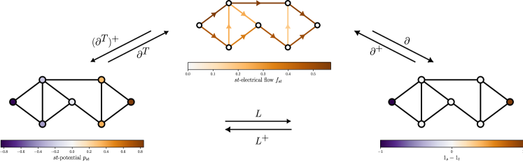
Figure 2: From right to left: the vector $1_{s}-1_{t}$, the electrical flow $f_{st}=\partial^{+}(1_{s}-1_{t})$, the potentials $p_{st}=L^{+}(1_{s}-1_{t})$, and the maps that connect them.

Let $G=(V,E,w)$ be a undirected, weighted graph with $n=|V|$ and $m=|E|$. The adjacency matrix is the matrix $A\in\mathbb{R}^{n\times n}$ where $A_{uv}=w(\{u,v\})$ if $\{u,v\}\in E$ and 0 otherwise. The degree matrix is the diagonal matrix $D\in\mathbb{R}^{n\times n}$ such that $D_{vv}=\sum_{u\in V}w(\{u,v\})=\deg(v)$, the degree of $v$. The Laplacian is the matrix $L=D-A\in\mathbb{R}^{n\times n}$. We index elements of the vectors in $\mathbb{R}^{n}$ and $\mathbb{R}^{m}$ by vertices and edges of $G$, where we assume a bijection between $V$ and $E$ and orthonormal bases of $\mathbb{R}^{n}$ and $\mathbb{R}^{m}$.

There is another common, equivalent way of defining the graph Laplacian. For each edge $\{s,t\}\in E$, fix an arbitrary order of its vertices $e=(s,t)$. The boundary matrix (aka signed incidence matrix) is the matrix $\partial:\mathbb{R}^{m}\to\mathbb{R}^{n}$ such that for an edge $e=(s,t)\in E$, the column $\partial 1_{e}=1_{s}-1_{t}$, where $1_{x}$ is the indicator column vector of a vertex or edge $x$. The graph Laplacian is $L=\partial W\partial^{T}$, where $W\in\mathbb{R}^{m\times m}$ is the diagonal weight matrix. To simplify notation, in this paper, we denote $\widetilde{\partial}=\partial W^{1/2}$, hence, $L=\widetilde{\partial}\widetilde{\partial}^{T}$.

For an edge $e=\{s,t\}\in E$, we use the notation $R_{e}$ and $B_{e}$ as shorthand for the effective resistance or biharmonic distance between its endpoints, i.e. $B_{e}=B_{st}$.

Electrical Interpretation of Effective Resistance

As the name suggests, the effective resistance has an interpretation in terms of electrical networks. For a graph $G$ with weights $w$, assume that each edge is a wire with resistance $w^{-1}_{e}$ (i.e. conductance $w_{e}$). If we insert a unit of current into $s$ and remove a unit of current from $t$, then $R_{st}$ is the resistance between $s$ and $t$.

There are other quantities associated with the electrical interpretation of effective resistance. The st-potential is the function $p_{st}:V\to\mathbb{R}$ defined $p_{st}=L^{+}(1_{s}-1_{t})$; in the interpretation, $p_{st}(v)$ is the voltage at the vertex $v$. The st-electrical flow between $s$ and $t$ is the function $f_{st}:E\to\mathbb{R}$ defined $f_{st}=\partial^{+}(1_{s}-1_{t})$; $f_{st}(e)$ is the amount of current flowing through the edge $e$. See Figure 2.

The following are well-known properties of $st$-potentials and $st$-electrical flows. For completeness, proofs of these lemmas can be found in Appendix B.

Lemma 2.1.

(Properties of $st$-potentials)

1. $B_{st}^{2}=\|p_{st}\|^{2}$

2. $R_{st}=p_{st}(s)-p_{st}(t)$

3. $s=\arg\max_{v\in V}p_{st}(v)$ and $t=\arg\min_{v\in V}p_{st}(v)$

4. $\sum_{v\in V}p_{st}(v)=0$

Lemma 2.2.

(Properties of $st$-electrical flows)

1. $R_{st}=f_{st}^{T}W^{-1}f_{st}=\sum_{e\in E}f_{st}^{2}(e)/w_{e}$

2. $f_{st}=\arg\min\{\|f\|^{2}:f:E\to\mathbb{R},\,\partial f=(1_{s}-1_{t})\}$

3 Formula for Biharmonic Distance of Edges

In this section, we prove a new formula for the biharmonic distance on edges of a graph in terms of a different Laplacian associated with the graph called the down Laplacianthat is closely related to the graph Laplacian. Recall that the graph Laplacian is defined $L=\partial W\partial^{T}:\mathbb{R}^{n}\to\mathbb{R}^{n}$. The down Laplacian is defined $L^{down}=W^{-1/2}\partial^{T}\partial W^{-1/2}=\widetilde{\partial}^{T}\widetilde{\partial}:\mathbb{R}^{m}\to\mathbb{R}^{m}$. Theorem 3.1 shows that the biharmonic distance of an edge is proportional to the diagonal entry of the down Laplacian. The proof of this theorem can be found in Appendix C.

Theorem 3.1.

Let $G=(V,E,w)$ be a graph, $e\in E$, and $L^{\mathrm{down}}$ the down Laplacian of $G$. Then

$$w_{e}\cdot B_{e}^{2}=(L^{\mathrm{down}})^{+}_{ee}=\|1_{e}^{T}\widetilde{\partial}^{+}\|,$$

where $1_{e}^{T}\widetilde{\partial}^{+}$ is the row of $\widetilde{\partial}^{+}$ that corresponds to $e$.

One reason this formula is interesting is because it parallels the fact that the diagonals of the pseudoinverse of the Laplacian $L_{vv}^{+}$ have useful properties and have been used as a centrality measure on vertices called current-flow closeness centrality or information centrality (Brandes & Fleischer, 2005; Stephenson & Zelen, 1989). We explore biharmonic distance as a centrality measure on edges in Section 4.1.

4 Biharmonic Distance and Electrical Flows

Recall (Lemma 2.2) that the $st$-electrical flow $f_{st}$ is related to the effective resistance between $s$ and $t$ as follows:

$$R_{st}=f_{st}^{T}W^{-1}f_{st}=\sum_{e\in E}\frac{f_{st}(e)^{2}}{w_{e}}.$$

As a corollary, the total resistance can also be defined using the electrical flows between all pairs of vertices $s$ and $t$.

$$R_{\operatorname{tot}}=\sum_{s,t\in V}\sum_{e\in E}\frac{f_{st}(e)^{2}}{w_{e}}$$

Reordering the sums gives the formula

$$R_{\operatorname{tot}}=\sum_{e\in E}\sum_{s,t\in V}\frac{f_{st}(e)^{2}}{w_{e}}.$$

Consider the quantity $\sum_{s,t\in V}f_{st}(e)^{2}/w_{e}$ for an edge $e$. At first glance, this seems like an interesting quantity and a good measure of how important an edge is to the global connectivity of a graph. If it is high, then many pairs of vertices use the edge $e$ to send current in their electrical flow, so it is important to the connection between these vertices. We call this quantity the squared electrical-flow centrality because of its connection to electrical-flow centrality; see Section 4.1 for details. Amazingly, the squared electrical-flow centrality is proportional to the squared biharmonic distance.

Theorem 4.1.

Let $G=(V,E,w)$ be a connected weighted graph with $n$ vertices. Let $e\in E$. Then

$$n\cdot w_{e}\cdot B_{e}^{2}=\sum_{s,t\in V}\frac{f_{st}(e)^{2}}{w_{e}}.$$

A proof of this theorem can be found in Appendix D.

4.1 Application: Edge Centrality

Edge centrality measures are ways of assigning values to the edges in a graph to determine which edges are most important to the global connectivity of a graph. Yi et al. (2018a) proposed to use the weighted squared biharmonic distance $nw_{e}^{2}B_{e}^{2}$ as a measure of edge centrality, while Li & Zhang (2018) implicitly use the biharmonic distance in their Kirchhoff Edge Centrality. Both of these papers proposed the biharmonic distance as a centrality measure because of its connection to the total resistance.

Theorem 4.1 provides further evidence why the squared biharmonic distance is a good measure of edge centrality. Intuitively, the biharmonic distance measures how important an edge is to the connection between all pairs of vertices in the graph. This is analogous to the edge-betweenness centrality, which measures what proportion of shortest paths between pairs of vertices an edge appears in. Furthermore, the squared current-flow centrality is closely related to the current-flow centrality $C_{e}$ introduced by Brandes & Fleischer (2005) (which is equivalent to random-walk betweenness introduced by Newman (2005)) defined

$$C_{e}=\sum_{s,t\in V}|f_{st}(e)|.$$

As the squared biharmonic distance of an edge in an unweighted graph is $nB_{e}^{2}=\sum_{s,t\in V}f^{2}_{st}(e)$, then $B_{e}^{2}$ and $C_{e}$ are comparable as they both measure the amount of current that flows through the edge $e$ in all-pairs electrical flows. This may explain some of the success of using the biharmonic distance as a centrality measure.

However, one advantage of the biharmonic distance over the current-flow centrality is computation time. Brandes & Fleischer (2005) gave an algorithm for computing the current-flow centrality of all edges in $O(n^{3}+mn\log n)$ time, where $O(n^{3})$ is the time needed to compute the pseudoinverse of an $n\times n$ matrix. In contrast, because $B_{st}=\sqrt{L_{ss}^{2+}+L_{tt}^{2+}-2L_{st}^{2+}}$, computing the biharmonic distance for all edges takes $O(n^{3}+m)$ time, as computing a single biharmonic distance takes $O(1)$ time after computing the pseudoinverse of the $L^{2}$ in $O(n^{3})$. Thus, excluding the time to invert the matrices, biharmonic distance is faster to compute than current-flow centrality. See Appendix H for an empirical comparison of these algorithms.

Furthermore, Yi et al. (2018a) observe that biharmonic distance can be efficiently approximated using random projections and fast solvers for linear systems in the Laplacian. This algorithm uses the fact that the biharmonic distance is a Euclidean distance, meaning it can be approximated by another Euclidean distance in a lower-dimensional space via random projection. As current-flow centrality is not a Euclidean distance, random projection techniques cannot be used. While computing the pseudoinverse of the Laplacian requires solving $n$ linear system in the Laplacian, approximating the biharmonic distances only requires solving $O(\log n)$ linear systems in the Laplacian. Combined with fast Laplacian solvers (Spielman & Teng, 2004), this algorithm takes $O(m\operatorname{poly}\log n)$ time to approximate the biharmonic distance of all edges.

4.2 Corollary: A Biharmonic Foster’s Theorem

A corollary to Theorem 4.1 is an analog of Foster’s theorem for biharmonic distance. Foster’s Theorem connects the effective resistances on the edges of the graph to the size of the graph, while the Biharmonic Foster’s Theorem connects the biharmonic distance on edges to the total resistance.

Theorem 4.2 (Foster’s Theorem (Foster, 1949)).

Let $G=(V,E,w)$ be a connected graph with $n$ vertices. Then

$$\sum_{e\in E}w_{e}R_{e}=n-1$$

Corollary 4.3 (Biharmonic Foster’s Theorem).

Let $G=(V,E)$ be a connected graph with $n$ vertices. Then

$$n\sum_{e\in E}w_{e}B_{e}^{2}=R_{\operatorname{tot}}$$

5 Biharmonic Distance and Cuts

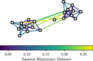
Figure 3: Theorems 5.3 and 5.4 suggest that edges crossing sparse cuts will have high biharmonic distance, which we can see in this example of a block stochastic graph.

In this section, we prove several result connecting the biharmonic distance on edges to the existence of sparse cuts in unweighted graphs. Our results are in terms of the isoperimetric ratio of a cut. The isoperimetric ratio is a way of measuring the sparsity of a cut, because it is lower the fewer the edges in the cut and the closer the cut is to dividing the graph in half. The isoperimetric ratio is commonly used to quantify the quality of a clustering, from the classic Cheeger inequality (Chung, 1997) to more recent analyses of spectral clustering algorihtms (Kannan et al., 2004; Lee et al., 2014).

Let $S\subset V$. Let $E(S,V\setminus S)=\{\{s,t\}\in E:s\in V,\,t\notin V\}$ be the edges leaving $S$. The isoperimetric ratioof $S$ is

$$\Theta(S)=\frac{n|E(S,V\setminus S)|}{|S||V\setminus S|}.$$

5.1 Biharmonic Distance on Cut Edges

Our first result is about cut edges of a graph. For a connected graph $G$, a cut edge is an edge $e$ such that $G\setminus\{e\}$ is disconnected. Theorem 5.1 shows that the squared biharmonic distance of a cut edge is the inverse isoperimetric ratio of its cut.

Theorem 5.1.

Let $G=(V,E)$ be a connected, unweighted graph. Let $e$ be a cut edge of $G$. Let $S\cup T=V$ be the connected components of $G\setminus\{e\}$. Then

$$B_{e}^{2}=\frac{|S||T|}{n}=\Theta(S)^{-1}.$$

Proofs for all theorems in this section are in Appendix E.

Comparision with Effective Resistance

Theorem 5.1 gives a good way to compare effective resistance to biharmonic distance. The effective resistance of a cut edge is always 1, so while the effective resistance reveals when an edge is a cut edge, it does not reveal anything about the cut and is the same whether the cut separates a single vertex or half the graph. In contrast, the biharmonic distance of a cut edge equals the inverse isoperimetric ratio of the cut, so in some sense, biharmonic distance reveals which cut edges are more important for connecting the graph. See Figure 1.

Theorem 5.2 (Folklore).

Let $G$ be an unweighted graph. Let $e$ be a cut edge. Then $R_{e}=1$

5.2 Biharmonic Distance on Edges and Sparse Cuts

Theorem 5.1 shows that the squared biharmonic distance of a cut edge equals the sparsity of the cut. In this section, we generalize this theorem to all cuts, not just cuts containing a single edge. First, Theorem 5.3 shows that the existence of a sparse cut implies the existence of an edge with high biharmonic distance. Conversely, Theorem 5.4 shows that the existence of an edge with high biharmonic distance implies the existence of a sparse cut. See Figure 3.

Theorem 5.3.

Let $G=(V,E)$ be a connected, unweighted graph. Let $S\subset V$. Then

$$\sum_{e\in E(S,V\setminus S)}B_{e}^{2}\geq\frac{|S||V\setminus S|}{|E(S,V\setminus S)|n}=\Theta(S)^{-1}.$$

In particular, there is an edge $e\in E(S,V\setminus S)$ such that $B_{e}^{2}\geq\frac{\Theta(S)^{-1}}{|E(S,V\setminus S)|}$.

Theorem 5.4.

Let $G=(V,E)$ be an unweighted graph. Let $\{s,t\}\in E$. Then there is a subset $S\subset V$ such that $s\in S$, $t\in V\setminus S$, and

$$B_{st}^{2}\in O(d_{\max}\Theta(S)^{-2}),$$

where $d_{\max}$ is the maximum degree of any vertex in $G$.

5.3 Application: Clustering Algorithms

The results in the previous section suggest two natural algorithms for graph clustering.

Biharmonic $k$-means

Theorem 5.3 intuitively suggests that vertices on opposite sides of a sparse cut likely have large biharmonic distance. This motivates a clustering algorithm that aims to separate vertices with large biharmonic distance. The $k$-means clustering algorithm minimizes the distance between points in the same cluster; however, $k$-means only can be applied to points in Euclidean space, not graphs. Fortunately, the biharmonic distance is a Euclidean metric. Namely, if we consider the points $p_{v}:=L^{+}1_{v}\in\mathbb{R}^{n}$, then $B_{st}=\|p_{u}-p_{v}\|$. Therefore, we can cluster a graph by performing $k$-means on the points $\{p_{v}:v\in V\}$. This idea has previously been proposed for effective resistance by Yen et al. (2005) and is analogous to the spectral clustering algorithm (Shi & Malik, 2000; Ng et al., 2001) that similarly embeds vertices into Euclidean space then clusters them with $k$-means. The proposed clustering algorithm is summarized in Algorithm 1.

We explore an alternative interpretation of this algorithm and compare it to spectral clustering in Appendix G.

Algorithm 1 Biharmonic $k$-Means (Graph $G$, int $k$)

1:  # Cluster the graph $G$ into $k$ clusters

2:  Compute $L^{+}$ # The columns of $L^{+}$ are the points $p_{v}$

3:  return $k$-means($L^{+}$)

Biharmonic Girvan-Newman Algorithm

Theorem 5.3 implies that the existence of a sparse cut implies an edge with large biharmonic distance. We now propose a graph clustering algorithm inspired by this intuition.

Our algorithm is an instance of the generic Girvan-Newman Algorithm (Girvan & Newman, 2002) for graph clustering, given below. The Girvan-Newman algorithm repeatedly removes the edge in a graph that maximizes some measure on the edges, typically a centrality measure. Our variant (Algorithm 2) will use the (squared) biharmonic distance as the measure on the edges.

Algorithm 2 Biharmonic Girvan-Newman (Graph $G$, int $k$)

  # Cluster the graph $G$ into $k$ clusters

  while $G$ has fewer than $k$ connected components do

     $e_{\max}\leftarrow\underset{e\in E}{\arg\max}B_{e}^{2}$

     $G\leftarrow G\setminus\{e_{\max}\}$

  end while

  return connected components of $G$

6 k-Harmonic Distance

So far, we have been concerned with the biharmonic distance as a variant of effective resistance. The biharmonic distance alters the definition of effective resistance by using the squared pseudoinverse $L^{2+}$ instead of the pseudoinverse $L^{+}$ and adding a square root. However, we can generalize the biharmonic resistance even further by considering arbitrary powers of the pseudoinverse $L^{k+}$. We define the k-harmonic distance between vertices $s$ and $t$ as

$$H_{st}^{(k)}=\sqrt{(1_{s}-1_{t})^{T}L^{k+}(1_{s}-1_{t})}.$$

The effective resistance between $s$ and $t$ is $R_{st}=(H_{st}^{(1)})^{2}$, and the biharmonic distance between $s$ and $t$ is $B_{st}=H_{st}^{(2)}$.

For the experimental part of this paper, we consider integer values of $k\geq 1$, but generally, $k$ can take any real value. In particular, $(L^{+})^{k}=L^{-k}$ for negative value of $k$, and $(L^{+})^{0}$ is the orthogonal projection onto $\operatorname{im}(L^{+})=\operatorname{im}(L)$.

6.1 Low-Rank Approximation

Another way to generalize effective resistance is to consider an approximation that only uses a subset of the eigenvectors of $L^{+}$. Since the Laplacian (and therefore all of it powers) are symmetric, we can spectrally decompose the pseudoinverse of $L^{k+}=\sum_{i=2}^{n}\frac{1}{\lambda_{i}^{k}}x_{i}x_{i}^{T}$. Using this decomposition, we can approximate $L^{k+}$ using only eigenvectors correspond to the the smallest $r$ eigenvalues, as these are the eigenvectors with the largest coefficients $1/\lambda_{i}^{k}$ in the spectral decomposition. We can then approximate the $k$-harmonic distance with this approximation of $L^{k+}$. The rank-r k-harmonic distance is defined

$$H^{k,r}_{s,t}=\sqrt{\sum_{i=2}^{r+1}\frac{1}{\lambda_{i}^{k}}(1_{s}-1_{t})^{T}x_{i}x_{i}^{T}(1_{s}-1_{t})}$$

This sort of low rank approximation is common practice in applied spectral graph theory, e.g. (Lipman et al., 2010).

The rank-$r$ $k$-harmonic distance allows us to place $k$-harmonic $k$-means clustering on a continuous spectrum between existing graph clustering algorithms. At one extreme of $k\to 0$, the coefficients of the eigenvalues $\lambda_{i}^{-k}\to 1$; therefore, we are clustering based on an unweighted embedding of the first $r$ eigenvectors. This is exactly the spectral clustering algorithm (Shi & Malik, 2000; Ng et al., 2001). At the other extreme of $k\to\infty$, the contribution of the smallest eigenvalue $\lambda_{2}$ dominates, so this is exactly the partitioning algorithm used in the proof of Cheeger’s Inequality (Cheeger, 1969; Chung, 1997).

6.2 A Foster’s Theorem for k-Harmonic Distance

Unfortunately, the $k$-harmonic distance is currently less interpretable than the effective resistance and biharmonic distance (although it is still useful in practice; see Section 7). However, some of our theorems for the biharmonic distance generalize to $k$-harmonics, even if they lose some of their interpretatiblity in the generalization.

For example, we prove a generalization of Theorem 4.1 (Theorem 6.1), noting that $f_{st}(e)=(\widetilde{\partial}1_{e})L^{+}(1_{s}-1_{t})$, which equals $1_{e}^{T}\widetilde{\partial}(\widetilde{\partial}^{+})^{T}\widetilde{\partial}^{+}(1_{s}-1_{t})=1_{e}^{T}\widetilde{\partial}^{+}(1_{s}-1_{t})$. Likewise, Theorem 6.2 is a generalization of the fact that $R_{st}$ is the 2-norm of the $st$-electrical flow.

Theorem 6.1.

Let $G=(V,E,w)$ be a connected weighted graph with $n$ vertices, let $e\in E$, and let $k\in\mathbb{R}$. Then

$$\sum_{s,t\in V}{\left((\widetilde{\partial}1_{e})^{T}(L^{+})^{k}(1_{s}-1_{t})\right)^{2}}=n\cdot w_{e}\cdot(H_{e}^{(2k)})^{2}.$$

Theorem 6.2.

Let $G=(V,E,w)$ be a connected weighted graph with $n$ vertices, let $s,t\in V$, and let $k\in\mathbb{R}$. Then

$$\sum_{e\in E}{\left((\widetilde{\partial}1_{e})^{T}(L^{+})^{k}(1_{s}-1_{t})\right)^{2}}=(H_{st}^{(2k-1)})^{2}.$$

From the theorems above, we prove the major result of this section, Theorem 6.3, that relates the $2k$-harmonic distance on the edges of a graph to all-pairs $(2k-1)$-harmonic distance. This generalizes the well-known Foster theorem (Theorem 4.2) and its biharmonic variant (Corollary 4.3) for $k=1/2$ and $k=1$, respectively.

Theorem 6.3 ($k$-harmonic Foster’s Theorem).

Let $G=(V,E,w)$ be a weighted graph, and let $k\in\mathbb{R}$. Then

$$\sum_{s,t\in V}(H_{st}^{(2k-1)})^{2}=n\cdot\sum_{e\in E}w_{e}\cdot(H_{e}^{(2k)})^{2}.$$

A proof of these theorems can be found in Appendix F.

7 Experiments

7.1 Centrality

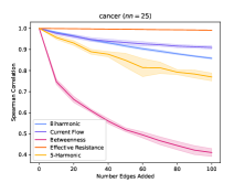
Figure 4: Left: The Spearman Rank Correlation Coefficient between different edge centrality measures on the 25-nearest neighbor graph of the Cancer dataset. Here BH is biharmonic distance, CF is current-flow centrality, B is betweenness centrality, ER is effective resistance, and 5H is 5-harmonic distance.
Right: The Spearman Rank Correlation Correlation between an edge centrality measure and the same edge centrality measure after a number of random edges were added. Experiments were repeated 5 times for each centrality measure. Results for more graphs can be found in Appendix J.

This section compares the biharmonic distance and $k$-harmonic distance against the other centrality measures current-flow centrality, betweenness centrality, and effective resistance. We compare them in two ways: correlation and resilience to changes in the graph. For both experiments, we use the $k$-nearest neighbor graphs for $k\in\{25,50,75,100\}$ of the Cancer (Zwitter & Soklic, 1988), Wine (Aeberhard & Forina, 1991), and Iris (Fisher, 1988) datasets from the UCI Machine Learning repository (Kelly et al., ). We use $k=5$ for the $k$-harmonic distance.

For the first experiment, we compare the ranking of the edges by the different centrality measures (e.g. the list of edges order from highest to lowest centrality) using the Spearman Rank Correlation Coefficient (Spearman, 1904).

For sparser graphs (fewer nearest neighbors $k$), the biharmonic distance is highly correlated with the current-flow centrality, which we might expect given their mutual connection to electrical flows. However, as $k$ increases, biharmonic distance tends to become less correlated with current-flow centrality and more correlated with effective resistance, while current-flow centrality tends to be more correlated with betweenness centrality. What is most surprising is that $5$-harmonic distance is often almost perfectly correlated with current-flow centrality. Our theoretical results do not posit any explanation for this behavior.

For the second experiment, we compare the original order of edges given by a centrality measure to the order given by the same centrality measure after adding a number of random edges. This experiment aims to test how resilient a centrality measure is to perturbations in the graph. The less the ordering of the edges changes, the more resilient the centrality measure is. This is a desirable property of a centrality measure as we would like the measure to be roughly the same given small changes in the input graph.

We found the effective resistance had the highest resilience, as the ordering was often nearly unchanged by adding edges. (This extreme resilience to noise was previously noted by Mavroforakis et al. (2015).) We also found that the biharmonic distance and current-flow centrality were the next most resilient to noise, followed by the 5-harmonic distance and then betweenness centrality.

Results for the 25-nearest neighbor graph of the Cancer dataset are given in Figure 4. Results for all graphs can be found in Appendix J.

7.2 Clustering

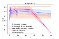
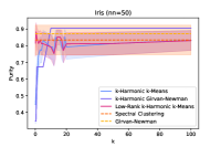
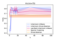
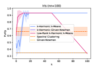
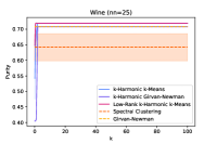
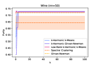
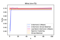
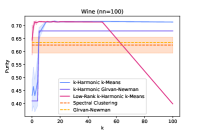
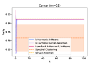
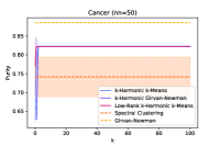
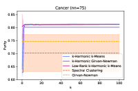
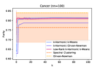
Figure 5: Plots of Purity vs. $k$ for $k$-harmonic clustering algorithms. Different plots correspond to nearest neighbor graphs of different datasets. Algorithms not parameterized by $k$ (i.e. Spectral Clustering and Girvan-Newman) are denoted with a dashed line. $k$-harmonic $k$-means, Low Rank $k$-harmonic $k$-means, and Spectral Clustering are averaged over 10 runs of $k$-means with different seeds.

This section compares the performance of our proposed $k$-harmonic $k$-means and $k$-harmonic Girvan-Newman algorithm against classical clustering methods. We also compare $k$-means clustering using the low-rank approximation of $k$-harmonic distance from Section 6.1. We compare our algorithms against the Spectral Clustering (Shi & Malik, 2000; Ng et al., 2001) and classical Girvan-Newman (Girvan & Newman, 2002) (using edge-betweenness centrality) clustering algorithms. As our computations of biharmonic and $k$-harmonic distances use the unnormalized Laplacian, we also use the unnormalized Laplacian for spectral clustering.

We performed experiments of our clustering algorithms on synthetic and real world data. For the synthetic datasets, we generate connected block stochastic graphs with simulated clusters by generating edges between vertices within clusters with a probability $p$ and edges between vertices in different clusters with a probability $q$. For real world data, we use the Breast Cancer (Zwitter & Soklic, 1988), Wine (Aeberhard & Forina, 1991), and Iris (Fisher, 1988) classification datasets from the UCI Machine Learning repository (Kelly et al., ). We create unweighted, undirected graphs from these datasets by building a $k$-nearest-neighbors graph for values of $k\in\{25,50,75,100\}$. For all algorithms using the $k$-harmonic distance, we used the values of $k\in\{0.5,1,2,3,...,20,50,100\}$. For low-rank $k$-harmonic $k$-means, we set the rank $r$ to be number of clusters we are returning. We evaluate all algorithms using cluster purity. For all algorithms using k-means, we use random initialization of the centroids and give an average over ten trials with a 95% confidence interval. Partial results of our experiments are given in Figure 5. The results of our experiments for all datasets and algorithm are given in Appendix K.

We observe from Figures 5, 2, 3, 4 and 5 in Appendix K that algorithms using $k$-harmonic distances may be useful for clustering and can achieve results that outperform spectral clustering. Moreover, biharmonic distance almost always outperforms effective resistance, and in almost all cases, $k$-harmonic clustering and $k$-harmonic Girvan-Newman algorithms achieve optimal results at a wide range of values of $k$ larger than 2. A potential explanation for the high performance for large $k$ is given in Appendix G.

Code Code can be found at: https://github.com/ll220/biharmonic-kharmonic-clustering.

8 Conclusion

We studied the biharmonic and $k$-harmonic distance on graphs. We proved several useful theoretical properties of the biharmonic distance. We also proposed and tested graph clustering algorithms inspired by these properties. We found that our algorithms performed better with biharmonic distance than effective resistance, as expected, and the best results were achieved for $k$-harmonic distance with $k>2$. As well, our algorithms often performed comparably or better than existing algorithms.

While our theoretical results were mostly for the biharmonic distance, our experimental results suggests that the $k$-harmonic distance is also useful for edge centrality and graph clustering. It is an open question whether the $k$-harmonic distance has similar theoretical properties to the biharmonic distance.

Likewise, most of our theoretical results are for the biharmonic distance of edges. It is an open question if the biharmonic distance between general pairs of vertices also have useful theoretical properties.

While our experimental results on clustering appear to perform best for $k>2$, it is an open question of how to pick the best $k$ for a particular graph. Our experiments suggest that different values of $k$ are required to achieve optimal results for different graph inputs. It would be interesting to observe the behavior for $k$-harmonic clustering algorithms on a wider range of graphs to determine the graph parameters that correlate with the best $k$ value.

Finally, we only compared biharmonic and $k$-harmonic distance to effective resistance for edge centrality and graph clustering. However, effective resistance has been used in many other areas of machine learning. (See Section 1 for examples.) Future work could explore using biharmonic and $k$-harmonic distance for these other applications.

Impact Statement

This paper presents work whose goal is to advance the field of Machine Learning. There are many potential societal consequences of our work, none which we feel must be specifically highlighted here.

Appendix A Bounds on Biharmonic Distance

In this section, we prove bounds on the biharmonic distance in unweighted graphs.

Theorem A.1 (Lower Bound).

Let $G=(V,E)$ be an unweighted connected graph with $n$ vertices. Let $s,t\in V$. Then

$$\frac{2}{n^{2}}\leq B_{st}^{2}$$

Proof.

This follows from the Courant-Fischer theorem. While the Courant-Fischer theorem is more general, in this context, we only need the following corollary of the main theorem: for a symmetric matrix $A$ with minimal non-zero eigenvalue $\lambda_{\min}$, then for any non-zero vector $x\perp\ker A$, $\lambda_{\min}\leq x^{T}Ax/x^{T}x$.

The eigenvalues of the Laplacian of $G$ are bound above by $n$, so the non-zero eigenvalues of $L^{+}$ are bound below by $\frac{1}{n}$ and the non-zero eigenvalues of $L^{2+}$ are bound below by $\frac{1}{n^{2}}$. Moreover, the vector $(1_{s}-1_{t})\perp\ker L$ as $\ker L$ is spanned by the all-ones vector. Therefore the squared biharmonic distance between any pair of vertices $s$ and $t$ is $B_{st}^{2}=(1_{s}-1_{t})^{T}L^{2+}(1_{s}-1_{t})\geq\frac{2}{n^{2}}$, with the factor of 2 coming from $(1_{s}-1_{t})^{T}(1_{s}-1_{t})$. ∎

As the eigenvalues of $L^{2+}$ are upper-bounded by $O(n^{4})$, we can use the Courant-Fischer theorem to similarly upper-bound the biharmonic distance by $B_{st}^{2}\in O(n^{4})$; however, we can use a different argument to show that $B_{st}^{2}\in O(n^{3})$.

Theorem A.2 (Upper Bound).

Let $G=(V,E)$ be an unweighted graph with $n$ vertices. Let $s,t\in V$. Then

$$B_{st}^{2}\leq n^{3}.$$

Proof.

By Lemma 2.1 Item 1, we know that $R_{st}=p_{st}(s)-p_{st}(t)$. Moreover, by combining Lemma 2.1 Items 2 and 3, we conclude that $p_{st}(s)$ is positive and $p_{st}(t)$ is negative, which implies that $|p_{st}(s)|,|p_{st}(t)|\leq R_{st}$. Further, Lemma 2.1 Item 2 implies that $|p_{st}(v)|\leq R_{st}$ for all $v\in V$. Therefore,

$$B_{st}^{2}=\|p_{st}\|_{2}^{2}\leq\sum_{v\in V}R_{st}^{2}=nR_{st}^{2}.$$

As $R_{st}\leq n-1$, then $B_{st}^{2}\leq n^{3}$ ∎

Theorem A.3 (Upper Bound on Edges).

Let $G=(V,E)$ be an unweighted graph with $n$ vertices. Let $e\in E$. Then

$$B_{e}^{2}\leq n.$$

Proof.

The proof of this theorem follows the same steps as Theorem A.2, except that we can derive a tighter upper bound as $R_{e}\leq 1$ for an edge $e$. ∎

A.1 Tight Examples

We now show that the bounds above are all tight up to a constant.

• Lower Bound Consider the complete graph $K_{n}$ on $n$ vertices. The Laplacian $L$ of $K_{n}$ has $n-1$ eigenvalues of value $n$, and $1$ eigenvalue of value 0; moreover, the eigenvector associated with the 0 eigenvalue is the all-ones vector 1 (Spielman, 2019, Lemma 6.1.1). As $(1_{s}-1_{t})^{T}1=0$ for any vertices $s$ and $t$, then $(1_{s}-1_{t})$ is an eigenvector of $L$ with eigenvalue $n$. Therefore, the squared biharmonic distance between any two vertices $s$ and $t$ is $B_{st}^{2}=(1_{s}-1_{t})^{T}L^{2+}(1_{s}-1_{t})=\frac{2}{n^{2}}$.

• Upper Bound Consider the path graph $P_{n+1}$ on the vertices $\{v_{0},\ldots,v_{n}\}$ for $n+1$ odd, and let $s=v_{0}$ and $t=v_{n}$ be the endpoints. The $st$-potential is the function $p_{st}(v_{i})=\frac{n}{2}-i$. Therefore, the squared biharmonic distance is $B^{2}_{st}=p_{st}^{T}p_{st}\in\Omega(n^{3})$.

• Upper Bound on Edges Consider the path graph $P_{n}$ on the vertices $\{v_{1},\ldots,v_{n}\}$ for $n$ even. Consider the center edge $e=\{v_{n/2},v_{n/2+1}\}$. This edge is a cut edge with $v_{n/2}\in S$ and $v_{n/2+1}\notin S$. Moreover, $|S|=\frac{n}{2}$ and $|V\setminus S|=\frac{n}{2}$. Therefore, by Theorem 5.1, $B^{2}_{e}=\frac{|S||V\setminus S|}{n}=\frac{n^{2}}{4n}=\Omega(n)$.

A.2 Bounds on k-Harmonic Distance

Given that we are able to prove bounds on the biharmonic distance, it is a natural question if these same bounds can be generalized to the $k$-harmonic distance. The answer is only partially. By this, we mean that the technique of using the Courant-Fischer theorem (ala the proof of Theorem A.1) generalizes to $k$-harmonic distance, but the more advanced techniques in Theorems A.2 and A.3 do not generalize to $k$-harmonic distances for $k>2$.

Theorem A.4.

Let $G=(V,E)$ be an unweighted graph. Let $s,t\in V$. Let $k\in R$. Then

$$\frac{2}{n^{k}}\leq(H_{st}^{(k)})^{2}\leq n^{2k}.$$

Appendix B Proofs from Section 2

See 2.1

Proof.

1. This follows from the definition of biharmonic distance and $st$-potentials.

2. This follows from the definition of effective resistance and $st$-potentials.

3. Recall for any vertex $v\in V$, $Lp_{st}(u)=\sum_{\{u,v\}\in E}w_{\{u,v\}}(p_{st}(u)-p_{st}(v))$. The $st$-potentials satisfy $Lp_{st}=1_{s}-1_{t}$. As all edge weights $w_{\{u,v\}}$ are positive, this means that for any vertex $u\in V\setminus\{s\}$, as $Lp_{st}(u)\leq 0$, then $u$ must have a neighbor that is strictly larger than it on $p_{st}$; thus, $u\neq\arg\max_{v\in V}p_{st}$. The only remaining possibility is that $s=\arg\max_{v\in V}p_{st}(v)$. We can prove $t=\arg\max_{v\in V}p_{st}(v)$ using a similar argument.

4. This follows as $\operatorname{im}L^{+}\perp 1$, the all-ones vector. As $p_{st}\in\operatorname{im}L^{+}$, then $p_{st}^{T}1=\sum_{v\in V}p_{st}(v)=0$. ∎

See 2.2

Proof.

1. This follows from the definition of effective resistance and $st$-electrical flows.

2. For any linear map $A$ and any vector $x\in\operatorname{im}A$, it is a property of the pseudoinverse that $A^{+}x$ is the minimum-norm vector that $A$ map to $x$. ∎

Appendix C Proofs from Section 3

C.1 Proof of Theorem 3.1

See 3.1

Proof.

We can express the left hand side as

$$w_{e}B_{e}^{2}= w_{e}(\partial 1_{e})^{T}L^{2+}\partial 1_{e}$$

$$= (\partial W^{1/2}1_{e})^{T}L^{2+}\partial W^{1/2}1_{e}$$

$$= (\widetilde{\partial}1_{e})^{T}L^{2+}\widetilde{\partial}1_{e}$$

$$= (1_{e}^{T}\widetilde{\partial}^{T})\left((\widetilde{\partial}^{+})^{T}\widetilde{\partial}^{+}(\widetilde{\partial}^{+})^{T}\widetilde{\partial}^{+}\right)(\widetilde{\partial}1_{e}),$$

where, throughout, we use the fact that $W^{-1}=W^{+}$ as $W$ is full-rank. Further, the operators $\widetilde{\partial}^{T}(\widetilde{\partial}^{T})^{+}=\widetilde{\partial}^{+}\widetilde{\partial}=\Pi_{\operatorname{im}(\widetilde{\partial}^{T})}$, where $\Pi_{\operatorname{im}(\widetilde{\partial}^{T})}$ is the projection onto $\operatorname{im}(\widetilde{\partial}^{T})$. As $\operatorname{im}(\widetilde{\partial})^{+}=\operatorname{im}(\widetilde{\partial})^{T}$, then $\widetilde{\partial}^{T}(\widetilde{\partial}^{T})^{+}\widetilde{\partial}^{+}=\widetilde{\partial}^{+}$ and $(\widetilde{\partial}^{T})^{+}\widetilde{\partial}^{+}\widetilde{\partial}=(\widetilde{\partial}^{T})^{+}$. Therefore, we can simplify the expression for $w_{e}B_{e}^{2}$ to

$$B_{e}^{2}=1_{e}^{T}\widetilde{\partial}^{+}(\widetilde{\partial}^{T})^{+}1_{e}=1_{e}^{T}(L^{\mathrm{down}})^{+}1_{e}=(L^{\mathrm{down}})^{+}_{ee}.\qed$$

Appendix D Proofs from Section 4

See 4.1

Proof.

It will be convenient to express $f_{st}(e)^{2}/w_{e}$ using vector notation.

$$\frac{f_{st}(e)^{2}}{w_{e}}=(1_{e}^{T}W^{-1/2}\partial^{+}(1_{s}-1_{t}))^{2}=(1_{e}^{T}\widetilde{\partial}^{+}(1_{s}-1_{t}))^{2}.$$

As $\operatorname{im}(\widetilde{\partial}^{+})=\operatorname{im}(\widetilde{\partial}^{T})$ and $\widetilde{\partial}^{T}(\widetilde{\partial}^{T})^{+}=\Pi_{\operatorname{im}(\widetilde{\partial}^{T})}$, the projection onto $\operatorname{im}(\widetilde{\partial}^{T})$, then $\widetilde{\partial}^{+}=\widetilde{\partial}^{T}(\widetilde{\partial}^{T})^{+}\widetilde{\partial}^{+}$. Therefore,

$$\frac{f_{st}(e)^{2}}{w_{e}}= (1_{e}^{T}\widetilde{\partial}^{+}(1_{s}-1_{t}))^{2}$$

$$= \left(1_{e}^{T}\widetilde{\partial}^{T}(\widetilde{\partial}^{T})^{+}\widetilde{\partial}^{+}(1_{s}-1_{t})\right)^{2}$$

$$= \left(1_{e}^{T}\widetilde{\partial}^{T}L^{+}(1_{s}-1_{t})\right)^{2}$$

$$= \left(1_{e}^{T}\widetilde{\partial}^{T}L^{+}(1_{s}-1_{t})\right)\left(1_{e}^{T}\widetilde{\partial}^{T}L^{+}(1_{s}-1_{t})\right)^{T}$$

$$= 1_{e}^{T}\widetilde{\partial}^{T}L^{+}(1_{s}-1_{t})(1_{s}-1_{t})^{T}L^{+}\widetilde{\partial}1_{e}.$$

Now, adding the sides for all pairs $s,t\in V$, we obtain

$$\sum_{s,t\in V}{\frac{f_{st}(e)^{2}}{w_{e}}}$$

$$= \sum_{s,t\in V}{\left(1_{e}^{T}\widetilde{\partial}^{T}L^{+}(1_{s}-1_{t})(1_{s}-1_{t})^{T}L^{+}\widetilde{\partial}1_{e}\right)}$$

$$= 1_{e}^{T}\widetilde{\partial}^{T}L^{+}\left(\sum_{s,t\in V}{(1_{s}-1_{t})(1_{s}-1_{t})^{T}}\right)L^{+}\widetilde{\partial}1_{e}.$$

The term $(1_{s}-1_{t})(1_{s}-1_{t})^{T}$ is the Laplacian of the graph with the single edge $\{s,t\}$. Hence, the sum $\sum_{s,t\in V}{(1_{s}-1_{t})(1_{s}-1_{t})^{T}}$ is the Laplacian of the complete (unweighted) graph $K_{n}$.

$$L_{K_{n}}=\sum_{s,t\in V}(1_{s}-1_{t})(1_{s}-1_{t})^{T}.$$

The eigenvalues of $L_{K_{n}}$ are all $n$, with the exception of the all-ones vector $1$, which is the eigenvector with eigenvalue $0$ (Spielman, 2019, Lemma 6.1.1). However, as $1\perp\operatorname{im}L^{+}$, then $L^{+}\widetilde{\partial}1_{e}$ is an eigenvector of $L_{K_{n}}$ with eigenvalue $n$. Therefore,

$$\sum_{s,t\in V}{\frac{f_{st}(e)^{2}}{w_{e}}}= 1_{e}^{T}\widetilde{\partial}^{T}L^{+}L_{K_{n}}L^{+}\widetilde{\partial}1_{e}$$

$$= n\cdot 1_{e}^{T}\widetilde{\partial}^{T}L^{+}L^{+}\widetilde{\partial}1_{e}$$

$$= n\cdot 1_{e}^{T}\partial^{T}W^{-1/2}L^{+}L^{+}\partial W^{-1/2}1_{e}$$

$$= w_{e}\cdot n\cdot 1_{e}^{T}\partial^{T}L^{+}L^{+}\partial 1_{e}$$

$$= w_{e}\cdot n\cdot B_{e}.\qed$$

Appendix E Proofs from Section 5

Lemma E.1 is a useful property of cuts and flows that will be important for proving the theorems in this section.

Lemma E.1.

Let $G=(V,E)$ be an unweighted graph. Let $s,t\in V$. Let $f:E\to\mathbb{R}$ such that $\partial f=1_{s}-1_{t}$. Let $S\subset V$ such that $s\in S$ and $t\notin S$. Then

$$\sum_{e\in E(S,V\setminus S)}|f(e)|\geq 1$$

Moreover, if $|E(S,V\setminus S)|=1$, then $\sum_{e\in E(S,V\setminus S)}|f(e)|=1$.

Proof.

Consider the sum $\sum_{v\in S}\partial f(v)$. As $\partial f(v)=0$ for any $v\in S\setminus\{s\}$, then $\sum_{v\in S}\partial f(v)=\partial f(s)=1$. Moreover, recall that the boundary map $\partial$ is obtained by choosing an (arbitrary) order $(u,v)$ for each edge $\{u,v\}\in E$. Therefore, we can write $\partial f(v)$ using this ordering on the edges as $\partial f(v)=\sum_{(u,v)\in E}f(\{u,v\})-\sum_{(v,u)\in E}f(\{v,u\})$. Therefore, if we write $\sum_{v\in S}\partial f(v)$ in terms of the value of $f$ on the edges, then for any edge $(u,v)$ with $u,v\in V$, the terms $f(\{u,v\})$ and $-f(\{v,u\})$ cancel, and we are left with

$$1= \sum_{v\in S}\partial f(v)$$

$$= \sum_{v\in S}\left(\sum_{(u,v)\in E}f(\{u,v\})-\sum_{(v,u)\in E}f(\{v,u\})\right)$$

$$= \sum_{e\in E(S,V\setminus S)}(\pm 1)f(e)$$

where the $\pm 1$ term depends on the order of the edge. Therefore, the absolute value $1\leq\sum_{e\in E(S,V\setminus S)}|f(e)|$. Moreover, if there is a single edge in $E(S,V\setminus S)$, we find that $1=\sum_{e\in E(S,V\setminus S)}|f(e)|$. ∎

See 5.1

Proof.

By Theorem 4.1, we know that $n\cdot B_{e}^{2}=\sum_{s,t\in V}f_{st}(e)^{2}$. We can decompose the right-hand side into three sums: $\sum_{s\in S}\sum_{t\in T}f_{st}(e)^{2}$, $\sum_{s,t\in S}f_{st}(e)^{2}$, and $\sum_{s,t\in T}f_{st}(e)^{2}$.

For the first sum $\sum_{s\in V}\sum_{t\in T}f_{st}(e)^{2}$, we know by Lemma E.1 that $|f_{st}(e)|=1$ as $|E(S,T)|=1$. Therefore, $\sum_{s\in V}\sum_{t\in T}f_{st}(e)^{2}=|S||T|$.

For the second and third sums, we will reuse some ideas from the proof of Lemma E.1. First, observe that if $s,t\in S$ or $s,t\notin S$, then $\sum_{v\in S}\partial f(s)=0$. Therefore, $\sum_{v\in S}\partial f(v)=\sum_{e\in E(S,T)}(\pm 1)f(e)=0$. As $|E(S,T)|=1$, then we conclude that $f(e)=0$ for $e\in|E(S,T)|$. Therefore, $\sum_{s,t\in S}f_{st}(e)^{2}=\sum_{s,t\in T}f_{st}(e)^{2}=0$.

Therefore, $n\cdot B_{e}^{2}=\sum_{s,t\in V}f_{st}(e)^{2}=|S||T|$ and the theorem follows. ∎

See 5.3

Proof.

Fix a pair of vertices $s\in S$ and $t\in V\setminus S$. Consider the electrical flow $f_{st}$. By Lemma E.1, we know that $f_{st}$ must send at least 1 unit of flow along the cut edges $E(S,V\setminus S)$, i.e.

$$\sum_{e\in E(S,V\setminus S)}|f_{st}(e)|\geq 1.$$

The left-hand side is the 1-norm on a vector, so we can apply the Cauchy-Schwarz inequality to bound

$$\sqrt{\sum_{e\in E(S,V\setminus S)}f^{2}_{st}(e)}$$

$$\geq \frac{1}{\sqrt{|E(S,V\setminus S)|}}\sum_{e\in E(S,V\setminus S)}|f_{st}(e)|$$

$$\geq \frac{1}{\sqrt{|E(S,V\setminus S)|}},$$

or equivalently,

$$\sum_{e\in E(S,V\setminus S)}f^{2}_{st}(e)\geq\frac{1}{|E(S,V\setminus S)|}.$$

We can combine this with Theorem 4.1 to get the following inequality.

$$\sum_{e\in E(S,V\setminus S)}B_{e}^{2}= \frac{1}{n}\sum_{e\in E(S,V\setminus S)}\sum_{s,t\in V}f_{st}(e)^{2}$$

$$\geq \frac{1}{n}\sum_{e\in E(S,V\setminus S)}\sum_{s\in S}\sum_{t\in V\setminus S}f_{st}(e)^{2}$$

$$\geq \frac{1}{n}\sum_{s\in S}\sum_{t\in V\setminus S}\frac{1}{|E(S,V\setminus S)|}$$

$$\geq \frac{|S||V\setminus S|}{n|E(S,V\setminus S)|}=\Theta(S)^{-1}\qed$$

To prove the converse, we use Cheeger’s Inequality (Lemma E.2), that, for any vector $x$, proves the existence of a cut whose sparsity is upper-bounded by the Rayleigh quotient of $x$ with the Laplacian.

Lemma E.2 (Cheeger’s Inequality, e.g. (Chung, 1997)).

Let $G=(V,E)$ be a graph. Let $x:V\to\mathbb{R}$. Let $d_{\max}$ be the maximum degree of a vertex in $G$. Then there is a subset of vertices $S\subset V$ such that

$$\frac{x^{T}Lx}{x^{T}x}\in\Omega(\Theta(S)^{2}d_{\max}^{-1}).$$

Moreover, $S=\{v\in V:x(v)\geq t\}$ for some $t\in\mathbb{R}$

Theorem E.3.

Let $G=(V,E)$ be an unweighted graph. Let $s,t\in V$. Then there is a subset $S\subset V$ such that $s\in S$, $t\in V\setminus S$, and

$$B_{st}^{2}/R_{st}\in O(d_{\max}\Theta(S)^{-2}).$$

Proof.

Consider the $st$-potentials $p_{st}=L^{+}(1_{s}-1_{t})$. By Lemma E.2, we can find a cut $S$ with sparsity $\frac{p_{st}^{T}Lp_{st}}{p_{st}^{T}p_{st}}\in\Omega(\Theta(S)^{2}/d_{\max})$. The denominator $p_{st}^{T}p_{st}=B_{st}^{2}$. To bound the numerator, we recall the identity $L^{+}=L^{+}LL^{+}$; then, the numerator is just the effective resistance:

$$p_{st}Lp_{st}= (1_{s}-1_{t})^{T}L^{+}LL^{+}(1_{s}-1_{t})$$

$$= (1_{s}-1_{t})^{T}L^{+}(1_{s}-1_{t})$$

$$= R_{st}$$

This implies that $\frac{R_{st}}{B_{st}^{2}}\in\Omega(\Theta(S)^{2}/d_{\max})$.

Finally, Lemma 2.1 shows that the maximum and minimum values of $p_{st}$ are achieved at $s$ and $t$. As $S$ is a superlevel set of $p_{st}$, then $s\in S$ and $t\in V\setminus S$. ∎

See 5.4

Proof.

This follows from Theorem E.3 by observing that $R_{st}\leq 1$ for an edge $\{s,t\}$. ∎

Appendix F Proofs from Section 6

See 6.1

Proof.

For any $s,t\in V$, we have

$$((\widetilde{\partial} 1_{e})^{T}(L^{+})^{k}(1_{s}-1_{t}))^{2}$$

$$= (\widetilde{\partial}1_{e})^{T}(L^{+})^{k}(1_{s}-1_{t})(1_{s}-1_{t})^{T}(L^{+})^{k}(\widetilde{\partial} 1_{e}).$$

Since the sum $\sum_{s,t\in V}{(1_{s}-1_{t})(1_{s}-1_{t})^{T}}$ is the Laplacian of the complete (unweighted) graph $K_{n}$,

$$L_{K_{n}}=\sum_{s,t\in V}(1_{s}-1_{t})(1_{s}-1_{t})^{T},$$

we obtain,

$$\sum_{s.v\in V} {\left((\widetilde{\partial}1_{e})^{T}(L^{+})^{k}(1_{s}-1_{t}))\right)^{2}}$$

$$= (\widetilde{\partial}1_{e})^{T}(L^{+})^{k}L_{K_{n}}(L^{+})^{k}(\widetilde{\partial}1_{e})$$

$$= n\cdot(\widetilde{\partial}1_{e})^{T}(L^{+})^{2k}(\widetilde{\partial}1_{e})^{T}.$$

The last inequality holds because the eigenvalues of $L_{K_{n}}$ are all $n$, with the exception of the all-$1$s vector denoted $1$, which is the eigenvector with eigenvalue $0$. However, as $1\perp\operatorname{im}(L^{+})^{k}$, then $(L^{+})^{k}(1_{u}-1_{v})$ is an eigenvector of $L_{K_{n}}$ if $k>0$ with eigenvalue $n$. The same fact is true for the case that $k=0$, as $1\perp(1_{u}-1_{v})$.

Finally, since $\widetilde{\partial}1_{e}=\sqrt{w_{e}}\cdot\partial 1_{e}$, we obtain

$$n\cdot(\widetilde{\partial}1_{e})^{T}(L^{+})^{2k}\widetilde{\partial}1_{e}=n\cdot w_{e}\cdot(H_{e}^{(2k)})^{2}\qed$$

See 6.2

Proof.

For any $e\in E$, we have

$$(1_{e}^{T}\widetilde{\partial}^{T}(L^{+})^{k}(1_{s}-1_{t}))^{2}$$

$$= (1_{e}^{T}\widetilde{\partial}^{T}(L^{+})^{k}(1_{s}-1_{t}))^{T}(1_{e}^{T}\cdot\widetilde{\partial}^{T}(L^{+})^{k}(1_{s}-1_{t}))$$

$$= (1_{s}-1_{t})^{T}(L^{+})^{k}\widetilde{\partial}1_{e}1_{e}^{T}\widetilde{\partial}^{T}(L^{+})^{k}(1_{s}-1_{t}).$$

Since the sum $\sum_{e\in E}{\widetilde{\partial}1_{e}1_{e}^{T}\widetilde{\partial}^{T}}=L$, the Laplacian of $G$, then

$$\sum_{e\in E} {\left((\widetilde{\partial}1_{e})^{T}(L^{+})^{k}(1_{s}-1_{t})\right)^{2}}$$

$$= (1_{s}-1_{t})^{T}(L^{+})^{k}L(L^{+})^{k}(1_{s}-1_{t})$$

$$= (1_{s}-1_{t})^{T}(L^{+})^{k-1}L^{+}(L^{+})^{k-1}(1_{s}-1_{t})$$

$$= (1_{s}-1_{t})^{T}(L^{+})^{2k-1}(1_{s}-1_{t})$$

$$= (H_{st}^{(2k-1)})^{2}\qed$$

See 6.3

Proof.

Consider

$$S:=\sum_{e\in E}\sum_{s,t\in V}{\left(1_{e}^{T}\widetilde{\partial}^{T}(L^{+})^{k}(1_{s}-1_{t})\right)^{2}}$$

By Theorem 6.1,

$$S=n\cdot\sum_{e\in E}w_{e}\cdot(H_{e}^{(2k)})^{2}.$$

By Theorem 6.2, when flipping the sums in $S$,

$$S =\sum_{s,t\in V}\sum_{e\in E}{\left(1_{e}^{T}\widetilde{\partial}^{T}(L^{+})^{k}(1_{s}-1_{t})\right)^{2}}$$

$$=\sum_{s,t\in V}(H_{st}^{(2k-1)})^{2}.$$

Therefore,

$$\sum_{s,t\in V}(H_{st}^{(2k-1)})^{2}=S=n\cdot\sum_{e\in E}w_{e}\cdot(H_{e}^{(2k)})^{2}\qed$$

Appendix G An Alternative Interpretation of the k-Harmonic k-Means Algorithm

In addition to the connection between biharmonic distance and sparse cuts (Theorems 5.4 and 5.3), another potential explanation for the success of the $k$-harmonic distance for clustering is its connection to the spectral clustering algorithm (Shi & Malik, 2000; Ng et al., 2001) and the higher-order Cheeger inequality (Louis et al., 2012; Lee et al., 2014). As mentioned in Section 6.1, the spectral clustering and $k$-harmonic $k$-means algorithms have some similarities. The spectral clustering algorithms performs $k$-means clustering on the embedding of the vertices using the first $k$ eigenvectors of the Laplacian. In contrast, our $k$-harmonic $k$-means performs $k$-means clustering on the embedding of the vertices using all eigenvectors of the Laplacian, except with the eigenvectors scaled by the inverse polynomial of their eigenvalue $\lambda_{i}^{-k/2}$. Therefore, the eigenvectors that most contribute to the distribution of the vertices are the ones with the smallest eigenvalues (as these have the largest coefficient $\lambda_{i}^{-k/2}$.) Moreover, the larger the value of $k$, the more the embedding is weighted towards the eigenvectors with the smallest eigenvalues.

Both algorithms embed the vertices using the eigenvectors of the Laplacian and give particular preference to the small eigenvectors in different ways, either by dropping the larger eigenvectors (in the case of spectral clustering) or by weighting the smaller eigenvector more heavily (in the case of $k$-harmonic $k$-means.) This idea of using the smallest eigenvectors to cluster the graph is also supported theoretically. The higher-order Cheeger inequality (Louis et al., 2012; Lee et al., 2014) proves that the ability to partition a graph into $k$ subsets of small isoperimetric ratio is upper bounded by the $k$th smallest eigenvector. Moreover, the algorithm to find this partition uses a projection of the $k$ smallest eigenvectors. This reinforce the idea of clustering based on the smallest eigenvectors.

The connection between spectral clustering and the effective resistance has also been posed as an explanation for the success of spectral clustering; see (Von Luxburg, 2007, Section 6.2).

Appendix H Empirical Analysis of Time to Compute Biharmonic Distance

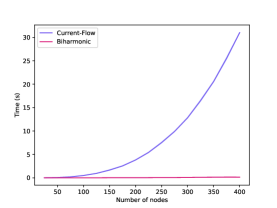
Figure 6: Time needed to compute biharmonic distance or current-flow centrality for all edges vs. number of vertices in the graph.

We compare the time needed to compute the biharmonic distance for all edges in a graph to the time needed to compute the current-flow centrality for all edges. We compare our implementation of the algorithm to compute biharmonic distance against the edge_current_flow_betweenness_centrality method from the NetworkX package (Hagberg et al., 2008). We use the naive $O(n^{3})$ time algorithm for biharmonic distance; see Section 4.1. We tested our method on Erdos-Renyi graphs with $n=25,50,...,400$ vertices and edge probability $p=0.5$. Results are averaged over 5 trials. Experiments were run on a 2018 MacBook Pro with a 2.3 GHz Quad-Core Intel Core i5 processor.

We found that our implementation was significantly faster than the NetworkX algorithm for current-flow centrality. While the difference in running times could be attributed to one of many differences in the implementation of the two algorithms, we feel reasonably confident this is a fair comparison as our implementation is a naive implementation with no significant optimizations.

Appendix I Figures

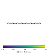
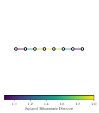
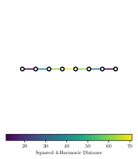
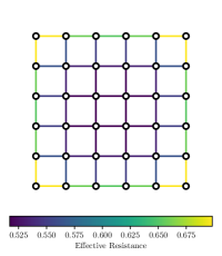
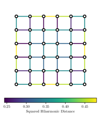
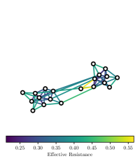
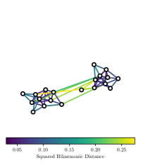
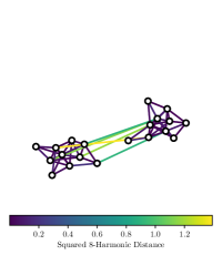
Figure 7: Examples of the squared $k$-harmonic distance for different graphs.

Appendix J Results from Centrality Experiments

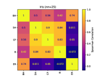
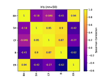
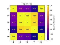
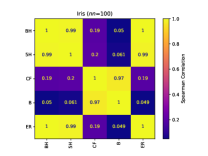
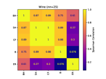
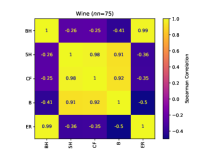
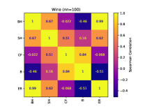
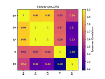
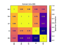
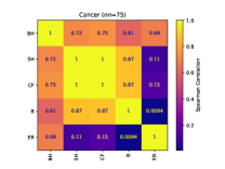
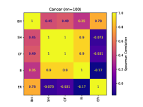
Figure 8: The Spearman Rank Correlation Coefficient between different centrality measures on the nearest neighbor graphs of various datasets. Here BH is biharmonic distance, CF is current-flow centrality, B is betweenness centrality, ER is effective resistance, and 5H is 5-harmonic distance.

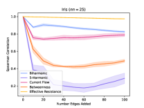
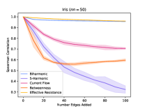
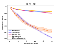
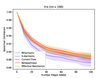
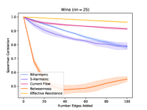
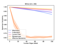
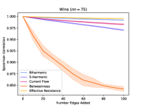
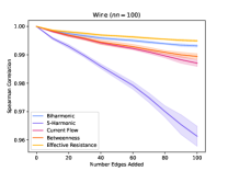
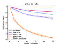
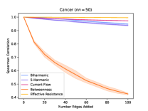
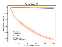
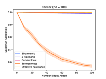
Figure 9: The Spearman Rank Correlation Correlation between an edge centrality measure and the same edge centrality measure after a number of random edges were added. Experiments were repeated 5 times for each centrality measure.

Appendix K Results from Clustering Experiments

Vertex Classification: Purity $(\uparrow)$
	Iris (nn=25)	Iris (nn=50)	Iris (nn=75)	Iris (nn=100)
$k$-harmonic Girvan-Newman
$k=0.5$	0.673	0.347	0.347	0.347
$k=1$	0.673	0.673	0.347	0.347
$k=2$	0.673	0.673	0.347	0.347
$k=5$	0.907	0.673	0.347	0.347
$k=10$	0.907	0.907	0.667	0.347
$k=20$	0.907	0.913	0.667	0.347
$k$-harmonic $k$-means
$k=0.5$	0.723 $\pm$ 0.119	0.541 $\pm$ 0.117	0.378 $\pm$ 0.072	0.417 $\pm$ 0.122
$k=1$	0.765 $\pm$ 0.087	0.572 $\pm$ 0.146	0.379 $\pm$ 0.072	0.421 $\pm$ 0.086
$k=2$	0.825 $\pm$ 0.098	0.740 $\pm$ 0.080	0.379 $\pm$ 0.072	0.477 $\pm$ 0.152
$k=5$	0.758 $\pm$ 0.069	0.833 $\pm$ 0.060	0.833 $\pm$ 0.000	0.437 $\pm$ 0.098
$k=10$	0.816 $\pm$ 0.056	0.793 $\pm$ 0.073	0.737 $\pm$ 0.059	0.873 $\pm$ 0.090
$k=20$	0.815 $\pm$ 0.056	0.793 $\pm$ 0.074	0.785 $\pm$ 0.055	0.933 $\pm$ 0.000
Low-Rank $k$-harmonic $k$-means
$k=0.5$	0.831 $\pm$ 0.081	0.884 $\pm$ 0.055	0.713 $\pm$ 0.046	0.700 $\pm$ 0.058
$k=1$	0.791 $\pm$ 0.094	0.845 $\pm$ 0.065	0.715 $\pm$ 0.055	0.722 $\pm$ 0.034
$k=2$	0.838 $\pm$ 0.007	0.813 $\pm$ 0.069	0.785 $\pm$ 0.055	0.876 $\pm$ 0.091
$k=5$	0.820 $\pm$ 0.077	0.813 $\pm$ 0.069	0.769 $\pm$ 0.059	0.906 $\pm$ 0.061
$k=10$	0.806 $\pm$ 0.070	0.793 $\pm$ 0.073	0.753 $\pm$ 0.060	0.933 $\pm$ 0.000
$k=20$	0.859 $\pm$ 0.051	0.812 $\pm$ 0.068	0.721 $\pm$ 0.055	0.933 $\pm$ 0.000
Girvan-Newman
-	0.907	0.873	0.667	0.346
Spectral Clustering
-	0.704 $\pm$ 0.051	0.835 $\pm$ 0.089	0.647 $\pm$ 0.028	0.661 $\pm$ 0.064

Table 2: Results of clustering experiments on nearest neighbor graphs of the Iris dataset (Fisher, 1988), evaluated using cluster purity. Averages were taken over ten trials for all algorithms using k-Means, provided with a 95% confidence interval. The Girvan-Newman algorithm is deterministic, so there is no confidence interval for these results. First, second, and third best results for each graph are colored.

Vertex Classification: Purity $(\uparrow)$
	Cancer (nn=25)	Cancer (nn=50)	Cancer (nn=75)	Cancer (nn=100)
$k$-harmonic Girvan-Newman
$k=0.5$	0.629	0.629	0.627	0.629
$k=1$	0.627	0.629	0.627	0.627
$k=2$	0.822	0.822	0.807	0.627
$k=5$	0.822	0.822	0.801	0.779
$k=10$	0.822	0.822	0.801	0.787
$k=20$	0.822	0.822	0.801	0.787
$k$-harmonic $k$-means
$k=0.5$	0.774 $\pm$ 0.071	0.739 $\pm$ 0.082	0.716 $\pm$ 0.082	0.637 $\pm$ 0.019
$k=1$	0.822 $\pm$ 0.000	0.803 $\pm$ 0.044	0.791 $\pm$ 0.041	0.767 $\pm$ 0.053
$k=2$	0.822 $\pm$ 0.000	0.822 $\pm$ 0.001	0.807 $\pm$ 0.000	0.803 $\pm$ 0.000
$k=5$	0.822 $\pm$ 0.000	0.822 $\pm$ 0.000	0.812 $\pm$ 0.002	0.808 $\pm$ 0.004
$k=10$	0.822 $\pm$ 0.000	0.822 $\pm$ 0.000	0.812 $\pm$ 0.002	0.808 $\pm$ 0.004
$k=20$	0.822 $\pm$ 0.000	0.822 $\pm$ 0.000	0.812 $\pm$ 0.002	0.811 $\pm$ 0.004
Low-Rank $k$-harmonic $k$-means
$k=0.5$	0.822 $\pm$ 0.000	0.821 $\pm$ 0.000	0.805 $\pm$ 0.002	0.809 $\pm$ 0.005
$k=1$	0.822 $\pm$ 0.000	0.821 $\pm$ 0.001	0.807 $\pm$ 0.001	0.810 $\pm$ 0.004
$k=2$	0.822 $\pm$ 0.000	0.822 $\pm$ 0.000	0.811 $\pm$ 0.001	0.810 $\pm$ 0.004
$k=5$	0.822 $\pm$ 0.000	0.822 $\pm$ 0.000	0.812 $\pm$ 0.002	0.809 $\pm$ 0.005
$k=10$	0.822 $\pm$ 0.000	0.822 $\pm$ 0.000	0.813 $\pm$ 0.002	0.809 $\pm$ 0.005
$k=20$	0.822 $\pm$ 0.000	0.822 $\pm$ 0.000	0.812 $\pm$ 0.002	0.808 $\pm$ 0.005
Girvan-Newman
-	0.824	0.886	0.747	0.840
Spectral Clustering
-	0.715 $\pm$ 0.077	0.741 $\pm$ 0.014	0.702 $\pm$ 0.133	0.763 $\pm$ 0.078

Table 3: Results of clustering experiments on nearest neighbor graphs of the Cancer dataset (Zwitter & Soklic, 1988), evaluated using cluster purity. Averages were taken over ten trials for all algorithms using k-Means, provided with a 95% confidence interval. The Girvan-Newman algorithm is deterministic, so there is no confidence interval for these results. First, second, and third best results for each graph are colored.

Vertex Classification: Purity $(\uparrow)$
	Wine (nn=25)	Wine (nn=50)	Wine (nn=75)	Wine (nn=100)
$k$-harmonic Girvan-Newman
$k=0.5$	0.404	0.399	0.404	0.410
$k=1$	0.410	0.399	0.404	0.410
$k=2$	0.708	0.607	0.404	0.410
$k=5$	0.708	0.730	0.680	0.680
$k=10$	0.708	0.730	0.680	0.680
$k=20$	0.708	0.730	0.680	0.680
$k$-harmonic $k$-means
$k=0.5$	0.656 $\pm$ 0.067	0.537 $\pm$ 0.085	0.423 $\pm$ 0.042	0.443 $\pm$ 0.060
$k=1$	0.688 $\pm$ 0.034	0.626 $\pm$ 0.088	0.463 $\pm$ 0.082	0.466 $\pm$ 0.074
$k=2$	0.719 $\pm$ 0.000	0.699 $\pm$ 0.040	0.537 $\pm$ 0.104	0.430 $\pm$ 0.063
$k=5$	0.719 $\pm$ 0.000	0.725 $\pm$ 0.000	0.701 $\pm$ 0.007	0.760 $\pm$ 0.002
$k=10$	0.719 $\pm$ 0.000	0.725 $\pm$ 0.000	0.699 $\pm$ 0.006	0.715 $\pm$ 0.002
$k=20$	0.719 $\pm$ 0.000	0.725 $\pm$ 0.000	0.697 $\pm$ 0.006	0.715 $\pm$ 0.002
Low-Rank $k$-harmonic $k$-means
$k=0.5$	0.719 $\pm$ 0.000	0.724 $\pm$ 0.004	0.696 $\pm$ 0.015	0.670 $\pm$ 0.021
$k=1$	0.719 $\pm$ 0.000	0.733 $\pm$ 0.002	0.699 $\pm$ 0.012	0.694 $\pm$ 0.021
$k=2$	0.719 $\pm$ 0.000	0.725 $\pm$ 0.000	0.698 $\pm$ 0.005	0.715 $\pm$ 0.002
$k=5$	0.719 $\pm$ 0.000	0.725 $\pm$ 0.000	0.703 $\pm$ 0.004	0.716 $\pm$ 0.002
$k=10$	0.719 $\pm$ 0.000	0.725 $\pm$ 0.000	0.701 $\pm$ 0.007	0.715 $\pm$ 0.002
$k=20$	0.719 $\pm$ 0.000	0.725 $\pm$ 0.000	0.697 $\pm$ 0.005	0.715 $\pm$ 0.002
Girvan-Newman
-	0.708	0.719	0.685	0.685
Spectral Clustering
-	0.642 $\pm$ 0.043	0.647 $\pm$ 0.028	0.661 $\pm$ 0.064	0.625 $\pm$ 0.030

Table 4: Results of clustering experiments on nearest neighbor graphs of the Wine dataset (Aeberhard & Forina, 1991), evaluated using cluster purity. Averages were taken over ten trials for all algorithms using k-Means, provided with a 95% confidence interval. The Girvan-Newman algorithm is deterministic, so there is no confidence interval for these results. First, second, and third best results for each graph are colored.

Vertex Classification: Purity $(\uparrow)$
	Synthetic (c=3,p=0.6,q=0.2)	Synthetic (c=5,p=0.7,q=0.15)
Girvan-Newman
-	0.347	0.800
$k$-harmonic Girvan-Newman
$k=0.5$	0.347	0.216
$k=1$	0.347	0.216
$k=2$	0.347	0.216
$k=5$	0.347	0.216
$k=10$	0.347	0.216
$k=20$	0.347	0.216
$k$-harmonic $k$-means
$k=0.5$	0.426 $\pm$ 0.074	0.282 $\pm$ 0.043
$k=1$	0.471 $\pm$ 0.107	0.304 $\pm$ 0.059
$k=2$	0.471 $\pm$ 0.107	0.327 $\pm$ 0.097
$k=5$	0.669 $\pm$ 0.156	0.567 $\pm$ 0.129
$k=10$	0.900 $\pm$ 0.114	0.940 $\pm$ 0.069
$k=20$	0.926 $\pm$ 0.098	0.880 $\pm$ 0.073
Low Rank $k$-harmonic $k$-means
$k=0.5$	0.903 $\pm$ 0.112	0.880 $\pm$ 0.100
$k=1$	0.867 $\pm$ 0.123	0.960 $\pm$ 0.060
$k=2$	0.967 $\pm$ 0.075	0.860 $\pm$ 0.100
$k=5$	0.867 $\pm$ 0.123	0.860 $\pm$ 0.118
$k=10$	0.988 $\pm$ 0.002	0.940 $\pm$ 0.070
$k=20$	0.960 $\pm$ 0.000	0.960 $\pm$ 0.060
Spectral Clustering
-	0.893 $\pm$ 0.109	0.899 $\pm$ 0.102

Table 5: Results of experiments on two synthetically generated stochastic block graphs with 50 vertices per cluster. The 3-cluster graph (left) was generated with edges within clusters occurring with probability $p$=0.6 and between clusters with probability $q$=0.2. The 5-cluster graph (right) is similarly generated, but with $p$=0.7 and $q$=0.15. Results were evaluated with cluster purity, and averages were taken over ten trials for all algorithms using $k$-means, provided with a 95% confidence interval. First, second, and third best results for each graph are colored.

References

- Aeberhard & Forina (1991) Aeberhard, S. and Forina, M. Wine. UCI Machine Learning Repository, 1991. DOI: https://doi.org/10.24432/C5PC7J.
- Alev et al. (2018) Alev, V. L., Anari, N., Lau, L. C., and Oveis Gharan, S. Graph clustering using effective resistance. In 9th Innovations in Theoretical Computer Science Conference (ITCS 2018). Schloss Dagstuhl-Leibniz-Zentrum fuer Informatik, 2018.
- Black et al. (2023) Black, M., Wan, Z., Nayyeri, A., and Wang, Y. Understanding oversquashing in gnns through the lens of effective resistance. In International Conference on Machine Learning, pp. 2528–2547. PMLR, 2023.
- Brandes & Fleischer (2005) Brandes, U. and Fleischer, D. Centrality measures based on current flow. In Annual symposium on theoretical aspects of computer science, pp. 533–544. Springer, 2005.
- Chakrabarti & Faloutsos (2006) Chakrabarti, D. and Faloutsos, C. Graph mining: Laws, generators, and algorithms. ACM Comput. Surv., 38(1):2–es, jun 2006. ISSN 0360-0300.
- Chandra et al. (1996) Chandra, A. K., Raghavan, P., Ruzzo, W. L., Smolensky, R., and Tiwari, P. The electrical resistance of a graph captures its commute and cover times. computational complexity, 6(4):312–340, Dec 1996. ISSN 1420-8954. doi: 10.1007/BF01270385. URL https://doi.org/10.1007/BF01270385.
- Cheeger (1969) Cheeger, J. A lower bound for the smallest eigenvalue of the laplacian. In Proceedings of the Princeton conference in honor of Professor S. Bochner, pp. 195–199, 1969.
- Chung (1997) Chung, F. R. Spectral graph theory, volume 92. American Mathematical Soc., 1997.
- Coifman & Lafon (2006) Coifman, R. R. and Lafon, S. Diffusion maps. Applied and computational harmonic analysis, 21(1):5–30, 2006.
- Ellens et al. (2011) Ellens, W., Spieksma, F. M., Van Mieghem, P., Jamakovic, A., and Kooij, R. E. Effective graph resistance. Linear algebra and its applications, 435(10):2491–2506, 2011.
- Fisher (1988) Fisher, R. A. Iris. UCI Machine Learning Repository, 1988. DOI: https://doi.org/10.24432/C56C76.
- Foster (1949) Foster, R. M. The average impedance of an electrical network. Contributions to Applied Mechanics (Reissner Anniversary Volume), 333, 1949.
- Ghosh et al. (2008) Ghosh, A., Boyd, S. P., and Saberi, A. Minimizing effective resistance of a graph. SIAM Rev., 50(1):37–66, 2008. doi: 10.1137/050645452. URL https://doi.org/10.1137/050645452.
- Girvan & Newman (2002) Girvan, M. and Newman, M. E. Community structure in social and biological networks. Proceedings of the national academy of sciences, 99(12):7821–7826, 2002.
- Hagberg et al. (2008) Hagberg, A. A., Schult, D. A., and Swart, P. J. Exploring network structure, dynamics, and function using networkx. In Varoquaux, G., Vaught, T., and Millman, J. (eds.), Proceedings of the 7th Python in Science Conference, pp. 11 – 15, Pasadena, CA USA, 2008.
- Herbster & Lever (2009) Herbster, M. and Lever, G. Predicting the labelling of a graph via minimum $p$-seminorm interpolation. In Annual Conference Computational Learning Theory, 2009. URL https://api.semanticscholar.org/CorpusID:7413410.
- Horak & Jost (2013) Horak, D. and Jost, J. Spectra of combinatorial laplace operators on simplicial complexes. Advances in Mathematics, 244:303–336, 2013.
- Kannan et al. (2004) Kannan, R., Vempala, S., and Vetta, A. On clusterings: Good, bad and spectral. J. ACM, 51(3):497–515, may 2004. ISSN 0004-5411. doi: 10.1145/990308.990313. URL https://doi.org/10.1145/990308.990313.
- (19) Kelly, M., Longjohn, R., and Nottingham, K. N. The UCI machine learning repository. URL https://archive.ics.uci.edu.
- Khoa & Chawla (2012) Khoa, N. L. D. and Chawla, S. Large scale spectral clustering using resistance distance and spielman-teng solvers. In Discovery Science: 15th International Conference, DS 2012, Lyon, France, October 29-31, 2012. Proceedings 15, pp. 7–21. Springer, 2012.
- Kirchhoff (1847) Kirchhoff, G. Ueber die auflösung der gleichungen, auf welche man bei der untersuchung der linearen vertheilung galvanischer ströme geführt wird. Annalen der Physik, 148:497–508, 1847.
- Klein & Randić (1993) Klein, D. J. and Randić, M. Resistance distance. Journal of Mathematical Chemistry, 12(1):81–95, Dec 1993. ISSN 1572-8897. doi: 10.1007/BF01164627. URL https://doi.org/10.1007/BF01164627.
- Lee et al. (2014) Lee, J. R., Gharan, S. O., and Trevisan, L. Multiway spectral partitioning and higher-order cheeger inequalities. J. ACM, 61(6), dec 2014. ISSN 0004-5411. doi: 10.1145/2665063. URL https://doi.org/10.1145/2665063.
- Li & Zhang (2018) Li, H. and Zhang, Z. Kirchhoff index as a measure of edge centrality in weighted networks: Nearly linear time algorithms. In Proceedings of the Twenty-Ninth Annual ACM-SIAM Symposium on Discrete Algorithms, pp. 2377–2396. SIAM, 2018.
- Lin (2022) Lin, Z. The biharmonic index of connected graphs. AIMS Mathematics, 7(4):6050–6065, 2022. ISSN 2473-6988. doi: 10.3934/math.2022337. URL https://www.aimspress.com/article/doi/10.3934/math.2022337.
- Lipman et al. (2010) Lipman, Y., Rustamov, R. M., and Funkhouser, T. A. Biharmonic distance. ACM Transactions on Graphics (TOG), 29(3):1–11, 2010.
- Louis et al. (2012) Louis, A., Raghavendra, P., Tetali, P., and Vempala, S. Many sparse cuts via higher eigenvalues. In Proceedings of the forty-fourth annual ACM symposium on Theory of computing, pp. 1131–1140, 2012.
- Lü & Zhou (2011) Lü, L. and Zhou, T. Link prediction in complex networks: A survey. Physica A: statistical mechanics and its applications, 390(6):1150–1170, 2011.
- Mavroforakis et al. (2015) Mavroforakis, C., Garcia-Lebron, R., Koutis, I., and Terzi, E. Spanning edge centrality: Large-scale computation and applications. In Proceedings of the 24th international conference on world wide web, pp. 732–742, 2015.
- Newman (2005) Newman, M. E. A measure of betweenness centrality based on random walks. Social networks, 27(1):39–54, 2005.
- Ng et al. (2001) Ng, A., Jordan, M., and Weiss, Y. On spectral clustering: Analysis and an algorithm. Advances in neural information processing systems, 14, 2001.
- Shi & Malik (2000) Shi, J. and Malik, J. Normalized cuts and image segmentation. IEEE Trans. Pattern Anal. Mach. Intell., 22(8):888–905, aug 2000. ISSN 0162-8828. doi: 10.1109/34.868688. URL https://doi.org/10.1109/34.868688.
- Spearman (1904) Spearman, C. The proof and measurement of association between two things. The American Journal of Psychology, 15(1), 1904.
- Spielman (2019) Spielman, D. Spectral and algebraic graph theory. Available at http://cs-www.cs.yale.edu/homes/spielman/sagt/sagt.pdf (2021/12/01), 2019.
- Spielman & Srivastava (2011) Spielman, D. A. and Srivastava, N. Graph sparsification by effective resistances. SIAM Journal on Computing, 40(6):1913–1926, 2011.
- Spielman & Teng (2004) Spielman, D. A. and Teng, S.-H. Nearly-linear time algorithms for graph partitioning, graph sparsification, and solving linear systems. In Proceedings of the thirty-sixth annual ACM symposium on Theory of computing, pp. 81–90, 2004.
- Stephenson & Zelen (1989) Stephenson, K. and Zelen, M. Rethinking centrality: Methods and examples. Social Networks, 11(1):1–37, 1989. ISSN 0378-8733. doi: https://doi.org/10.1016/0378-8733(89)90016-6. URL https://www.sciencedirect.com/science/article/pii/0378873389900166.
- Summers et al. (2015) Summers, T., Shames, I., Lygeros, J., and Dörfler, F. Topology design for optimal network coherence. In 2015 European Control Conference (ECC), pp. 575–580. IEEE, 2015.
- Teixeira et al. (2013) Teixeira, A. S., Monteiro, P. T., Carriço, J. A., Ramirez, M., and Francisco, A. P. Spanning edge betweenness. In Workshop on mining and learning with graphs, volume 24, pp. 27–31. Citeseer, 2013.
- Velingker et al. (2024) Velingker, A., Sinop, A., Ktena, I., Veličković, P., and Gollapudi, S. Affinity-aware graph networks. Advances in Neural Information Processing Systems, 36, 2024.
- Von Luxburg (2007) Von Luxburg, U. A tutorial on spectral clustering. Statistics and computing, 17:395–416, 2007.
- Wei et al. (2021) Wei, Y., Li, R.-h., and Yang, W. Biharmonic distance of graphs. arXiv preprint arXiv:2110.02656, 2021.
- Yen et al. (2005) Yen, L., Vanvyve, D., Wouters, F., Fouss, F., Verleysen, M., Saerens, M., et al. clustering using a random walk based distance measure. In ESANN, pp. 317–324, 2005.
- Yi et al. (2018a) Yi, Y., Shan, L., Li, H., and Zhang, Z. Biharmonic distance related centrality for edges in weighted networks. In IJCAI, pp. 3620–3626, 2018a.
- Yi et al. (2018b) Yi, Y., Yang, B., Zhang, Z., and Patterson, S. Biharmonic distance and performance of second-order consensus networks with stochastic disturbances. In 2018 Annual American Control Conference (ACC), pp. 4943–4950. IEEE, 2018b.
- Yi et al. (2021) Yi, Y., Yang, B., Zhang, Z., Zhang, Z., and Patterson, S. Biharmonic distance-based performance metric for second-order noisy consensus networks. IEEE Transactions on Information Theory, 68(2):1220–1236, 2021.
- Zhang et al. (2023) Zhang, B., Luo, S., Wang, L., and He, D. Rethinking the expressive power of gnns via graph biconnectivity. arXiv preprint arXiv:2301.09505, 2023.
- Zhu et al. (2003) Zhu, X., Ghahramani, Z., and Lafferty, J. Semi-supervised learning using gaussian fields and harmonic functions. In Proceedings of the Twentieth International Conference on International Conference on Machine Learning, ICML’03, pp. 912–919. AAAI Press, 2003. ISBN 1577351894.
- Zwitter & Soklic (1988) Zwitter, M. and Soklic, M. Breast Cancer. UCI Machine Learning Repository, 1988. DOI: https://doi.org/10.24432/C51P4M.