Sequential Monte Carlo for Cut-Bayesian Posterior Computation

Abstract

We propose a sequential Monte Carlo (SMC) method to efficiently and accurately compute cut-Bayesian posterior quantities of interest, variations of standard Bayesian approaches constructed primarily to account for model misspecification. We prove finite sample concentration bounds for estimators derived from the proposed method along with a linear tempering extension and apply these results to a realistic setting where a computer model is misspecified. We then illustrate the SMC method for inference in a modular chemical reactor example that includes submodels for reaction kinetics, turbulence, mass transfer, and diffusion. The samples obtained are commensurate with a direct-sampling approach that consists of running multiple Markov chains, with computational efficiency gains using the SMC method. Overall, the SMC method presented yields a novel, rigorous approach to computing with cut-Bayesian posterior distributions.

1 Introduction

Models of complex physical systems are often constructed via the coupling of multiple submodels where each represents a distinct, salient process. Submodels may entail their own experimental data, physical parameters, and a simulator of the subprocess being represented, all of which can be used for statistical modeling and inference. For example, Figure 1 illustrates the structure of an ethylene-oxide reactor model consisting of coupled submodels where each submodel corresponds to a relevant physical subprocess, such as turbulence, reaction kinetics, mass transfer, and diffusion. Standard Bayesian inference, especially with the aid of hierarchical models, is a powerful way to perform uncertainty quantification within physical systems such as the ethylene-oxide reactor illustrated. Nonetheless, modern Bayesian statistics has seen the development of cut-Bayesian posteriors for modular inference (Bayarri et al.,, 2009; Plummer,, 2015; Jacob et al.,, 2017; Carmona and Nicholls,, 2020; Yu et al.,, 2021; Frazier and Nott,, 2022), variations of standard approaches meant primarily to dampen the pernicious effects of model misspecification. Despite many recent developments in modular inference, computation can be a major impediment for the use of cut-Bayesian posteriors and is an active area of research. Our main objective is to introduce novel sequential Monte Carlo (SMC) methods for efficiently computing with cut-Bayesian posterior distributions along with finite-sample theoretical results that underpin the concentration of resultant estimators.

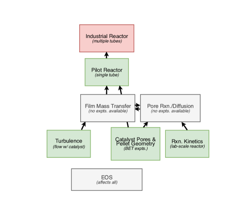
Figure 1: Components of a prototypical ethylene-oxide reactor model intended for demonstrating modular Bayesian inference, including the SMC method for cut-Bayes computation that is the subject of this paper. Green coloring indicates submodels for which experimental data exists, whereas gray corresponds to submodels that lack data. The top red model depicts the integration of multiple reactor tubes into a new design for which pure prediction would be required.

While we will precisely define what is meant by a cut-Bayesian posterior distribution in the following section, the essential idea of this modeling strategy is to fix distributions over some subset of the important parameters, or to only use some subset of the available experimental data and submodels to infer a distribution over said parameters. Subsequently, the associated uncertainty of these fixed distribution parameters is integrated out through a mixture when performing standard Bayesian inference over the remaining parameters of interest. Throughout, we will refer to the parameters with a fixed distribution as cut parameters and their corresponding fixed distribution as the cut distribution.

While our focus is computation, we provide some of the major arguments that have been made in favor of cut-Bayesian posteriors for context. Perhaps the most commonly cited justification is that of model misspecification; some submodels could be poorly specified, and it makes sense to use data only from the well-specified submodels in inferring parameters; this approach has sometimes also been referred to as feedback cutting. Second, it is common practice to use a plug-in point estimate for one or more parameters when there are many parameters to infer, as a way to mitigate complexity of the problem. However, the plug-in method inherently ignores uncertainty of the fixed parameter – instead, fixing a distribution over the parameter via cut Bayes provides a viable alternative to a full Bayesian approach that incorporates uncertainty for all parameters of interest. While fixing a parameter that does not provide much sensitivity could be appropriate, the same does not hold for sensitive parameters. A third, related motivation is computational complexity; for instance, a Markov chain Monte Carlo (MCMC) method may mix substantially better when working with fewer parameters than a full parameter set, for instance by avoiding non-identifiability. These and additional motivations are explicated in the work of Bayarri et al., (2009), Plummer, (2015), and Carmona and Nicholls, (2020), amongst others.

Despite sound justification for the use of cut-Bayes methodology, sampling from or approximating the cut-Bayesian posterior distribution can be an onerous computational difficulty. As outlined in Plummer, (2015), the ideal standard is to run many Markov chains long enough to explore the posterior distribution conditional on draws of the cut parameters, an approach we will refer to as direct sampling. This procedure yields exact samples from a cut-Bayesian posterior distribution in contrast to sampling from cut distributions within an MCMC routine – what Plummer, (2015) refers to as naive cut, which is not guaranteed to converge to the target distribution. However, running many Markov chains could take an unrealistic amount of time to complete, even in a parallel environment, given how many iterations may be needed to mix for even a single chain. As an alternative, Plummer, (2015) puts forth a heuristic approach dubbed tempered cut which takes small steps at each iteration for the cut parameter.

Besides the work of Plummer, (2015), there is some recent literature on computing or approximating cut-Bayesian posterior distributions. One such contribution is the unbiased MCMC method of Jacob et al., (2020), which is parallel and relies on maximal couplings of Markov chain proposals to ensure distinct chains meet. Additionally, Liu and Goudie, (2021) present a method for approximating the cut posterior distribution that improves on the tempered cut method of Plummer, (2015) and relies on stochastic approximation Monte Carlo (Liang et al.,, 2007). Yu et al., (2021) and Carmona and Nicholls, (2022) have developed variational inference for cut-Bayesian posterior computation. Baldé et al., (2023) use Gaussian-process emulation to approximate the posterior distribution conditional on cut parameters along with a linearity assumption for a coupled model. In comparison, to our knowledge, the method presented is the first development of the theory and application of SMC for computing with a cut-Bayesian posterior distribution. Some main features of the SMC method presented are that it:

1. yields estimators that concentrate around the true cut-Bayes posterior quantities with specific finite sample bounds,

2. does not require Gaussian or variational approximations to the posterior distribution conditional on cut parameters, and

3. does not assume linearity of functions, for instance, in the simulator.

The paper is structured as follows. Section 2 provides formal background for cut-Bayesian posterior distributions, SMC in general, and a SMC method with a linear tempering extension presented for computing cut-Bayesian posterior expectations; Theorem 1 and Corollary 1 provide finite-sample concentration results for the associated estimators of these methods. Moreover, Section 3 includes a detailed treatment of a specific instance of cut Bayes that could arise for a misspecified computer model. For this example, the posterior distribution of calibration parameters conditional on the cut parameters is normal with a mean prescribed by a general function of the cut parameters and data; finite sample complexity results are given for this specific case. The application of SMC to a cut-Bayesian posterior in the ethylene-oxide reactor modular example is presented in Section 4 as an illustration on an actual scientific model. We review our main findings and suggest future avenues for work in Section 5 and conclude.

2 Background, SMC Method, and Concentration

We begin by reviewing the definition of cut-Bayesian posteriors and SMC methodology in general. Then we set forth a specific SMC method for computing with cut-Bayesian posteriors and provide concentration results for SMC-based estimators of cut-Bayesian posterior quantities. We then show how a linear tempered variant of the SMC method can be employed that may allow for less computational burden. We follow up in the subsequent section with an example of how the theoretical results can be applied to a setting where there is model misspecification, for instance with computer models in which the conditional posterior takes a Gaussian form.

2.1 Cut-Bayesian Posteriors

Consider the set of parameters $(\nu,\theta)$ where $\nu\in\mathcal{X}^{d_{\nu}}$ and $\theta\in\mathcal{X}^{d}$. Let $\mathbf{y}=(y_{1},\ldots,y_{n})$ and suppose

$$\nu\sim p_{\nu}(\cdot)\quad\quad\mathbf{y}\mid\nu,\theta\sim p_{y}(\cdot\mid\nu,\theta).$$

Throughout, we refer to $\nu$ as the cut parameter(s) and $\theta$ as the calibration parameter(s). Often $p_{\nu}$ is presented as a posterior distribution corresponding to a separate submodel, though $p_{\nu}$ could be provided by domain experts without explicit reference to a posterior distribution or experimental data. We refer to $p_{\nu}$ as the cut distribution. The standard Bayesian posterior is given by:

$$\pi(\nu,\theta\mid\mathbf{y})=\pi(\nu\mid\mathbf{y})\pi(\theta\mid\mathbf{y},\nu)=\frac{p_{y}(\mathbf{y}\mid\nu,\theta)p_{\theta}(\theta\mid\nu)p_{\nu}(\nu)}{m(\mathbf{y})},$$ (1)

where $p_{\theta}$ denotes a prior distribution for $\theta$ and $m(\mathbf{y})$ is the marginal distribution for $\mathbf{y}$. Typically $\theta$ and $\nu$ are assumed independent apriori in which case $p_{\theta}(\theta\mid\nu)=p_{\theta}(\theta)$. When $p_{y}$ is misspecified, updating $\nu$ using $\mathbf{y}$ can lead to poor estimates of $\theta$ (Bayarri et al.,, 2009; Plummer,, 2015). This is a primary reason we may choose to not update $\nu$ using $\mathbf{y}$, leading to the cut-Bayes posterior:

$$\pi^{cut}(\nu,\theta\mid\mathbf{y})=p_{\nu}(\nu)\pi(\theta\mid\mathbf{y},\nu)=\frac{p_{y}(\mathbf{y}\mid\nu,\theta)p_{\theta}(\theta\mid\nu)p_{\nu}(\nu)}{p_{y}(\mathbf{y}\mid\nu)}.$$ (2)

The distributions (1) and (2) differ due to the difference in normalizing constants, with the term $p_{y}(\mathbf{y}\mid\nu)$ depending on $\nu$. The dependence of the normalizing constant on $\nu$ in the cut-Bayesian posterior prohibits sampling from (2) using standard MCMC methods (e.g. Metropolis-Hastings).

The direct-sampling approach from (2) (referred to as multiple imputation in Plummer, (2015)) is accomplished by first sampling $\nu\sim p_{\nu}$ and then sampling from the conditional distribution $\pi(\theta\mid\mathbf{y},\nu)$. If an MCMC method is used to sample from the conditional posterior, obtaining samples from (2) involves running $S$ distinct Markov chains conditional on different $\nu$ values. However, such a sampling strategy can quickly become infeasible if draws from $\pi(\theta\mid\mathbf{y},\nu)$ are expensive, for instance due to a long time for each Markov chain to mix. We propose an SMC method to sample from the cut-Bayesian posterior efficiently.

2.2 SMC

SMC methods (“particle filters”) are a class of algorithms designed to sequentially sample from a sequence of distributions $\mu_{0},\ldots,\mu_{S}$. For example, in filtering problems $\mu_{s}$ may be the posterior distribution of the state of a hidden Markov model conditional on the observation process. In Bayesian inference problems, $\mu_{S}$ may be the posterior distribution of a static parameter and $\mu_{s}\propto\mu^{\beta_{s}}_{S}$ for a sequence of inverse temperatures $\beta_{0}<\beta_{1}<\ldots<\beta_{S}=1$. Asymptotic properties of SMC algorithms have been studied extensively (Chopin,, 2004; Del Moral et al.,, 2012). Finite sample properties of SMC methods were given more recently in Marion et al., (2023). SMC algorithms are appealing in that they provide natural estimates of normalizing constants and can be adapted to parallel computing environments easily (Durham and Geweke,, 2014). In addition, they have been shown to perform well even in the presence of multimodality (Paulin et al.,, 2019; Mathews and Schmidler,, 2024).

An SMC algorithm is initialized by first obtaining samples (called particles) from $\mu_{0}$. Having obtained particles approximately drawn from $\mu_{s-1}$, a combination of resampling and MCMC methods are used to propagate particles forward to obtain samples approximately drawn from $\mu_{s}$. Critical to the success of SMC algorithms is the “closeness” of adjacent distributions $\mu_{s-1}$ and $\mu_{s}$, and defining a sequence of distributions that enables efficient sampling is challenging. Here, $\mu_{s}=\pi(\theta\mid\mathbf{y},\nu_{s})$, where $\nu_{s}$ is a sample from the cut distribution $p_{\nu}$. Consequently, $\mu_{s}$ is itself random and there is no natural ordering of the distributions without further knowledge of the form of $\pi(\theta\mid\mathbf{y},\nu_{s})$. Note that this setup can be viewed as a special case of a hidden Markov model, where $\nu_{s}$ corresponds to the hidden state and $\mu_{s}$ the emission probability distribution; here $\nu_{0:S}$ are independent and we are only interested in a fixed time interval of length $S$. Consequently, known finite sample bound results for SMC methods do not readily apply, and it is not immediately clear how the properties of $p_{\nu}$ change the complexity of the SMC algorithm. Our approach is to leverage concentration properties of $\nu_{0:S}$ so that particles approximately drawn from $\pi(\theta\mid\mathbf{y},\nu_{i})$ provide a close approximation of $\pi(\theta\mid\mathbf{y},\nu_{j})$ for $i\neq j$. In the following section, we give precise conditions under which this SMC algorithm provides an efficient stochastic approximation method for estimating expectations under $\pi^{cut}$.

2.3 Cut-Bayes SMC Method

With an SMC background established, we are now ready to introduce the SMC cut-Bayes method. Assume that we can obtain

$$\nu_{0:S}:=(\nu_{0},\ldots,\nu_{S})\overset{iid}{\sim}p_{\nu}.$$ (3)

We note that in practice (3) may only be “approximately” achieved by running a Markov chain targeting $p_{\nu}$ for a sufficient length of time. In our application (Section 4), $p_{\nu}$ is a known distribution (e.g. uniform) where (3) can be achieved exactly. The goal is to efficiently sample from $\mu_{0},\ldots,\mu_{S}$, where $\mu_{s}(\theta):=\pi(\theta\mid\mathbf{y},\nu_{s})$. Write $\mu_{s}(\theta)=q_{s}(\theta)/Z_{s}$, where $Z_{s}$ denotes the normalizing constant of $\mu_{s}(\theta)$. Denote the importance weights $w_{s}(\theta):=q_{s}(\theta)/q_{s-1}(\theta)$ and define their corresponding empirical average as

$$\bar{w}_{s}(\theta^{1}_{s-1},\ldots,\theta^{N}_{s-1})=\bar{w}_{s}=\frac{1}{N}\sum^{N}_{i=1}w_{s}(\theta^{i}_{s-1}).$$

Conditional on $\nu_{0:S}$, the algorithm we consider is a standard SMC algorithm:

1. Sample $\nu_{0:S}\overset{iid}{\sim}p_{\nu}$

2. Sample $\theta^{1:N}_{0}:=(\theta^{1}_{0},\ldots,\theta_{0}^{N})\overset{iid}{\sim}\mu_{0}$

3. For $s=1,\ldots,S$:

   1. Sample $\tilde{\theta}^{1:N}_{s}:=(\tilde{\theta}^{1}_{s},\ldots,\tilde{\theta}^{N}_{s})$, where

      $$\tilde{\theta}^{i}_{s}=\theta^{j}_{s-1}\text{ with probability }\frac{w_{s}(\theta^{j}_{s-1})}{N\bar{w}_{s}}$$

   2. Sample $\theta^{1:N}_{s}:=(\theta^{1}_{s},\ldots,\theta^{N}_{s})$, where

      $$\theta^{i}_{s}\sim K^{t}_{s}(\tilde{\theta}^{i}_{s},\cdot),$$

where $K_{1},K_{2},\ldots,K_{S}$ are a set of Markov kernels assumed to be ergodic and $K_{s}$ is $\mu_{s}$-invariant. The estimate of $\operatorname{\mathbb{E}}_{\pi^{cut}}[g]$ is given by

$$\hat{g}_{\text{SMC}}:=\frac{1}{S+1}\sum^{S}_{s=0}\left(\frac{1}{N}\sum^{N}_{i=1}g(\nu_{s},\theta^{i}_{s})\right),$$ (4)

for a measurable function $g(\theta,\nu)$. The following theorems give conditions under which $\hat{g}_{\text{SMC}}$ concentrates around $\operatorname{\mathbb{E}}_{\pi^{cut}}[g]$ for $g$ such that $|g|\leq 1$. Before stating these, we first fix some notation. Going forward, we let $\operatorname{\mathbb{P}}$ and $\operatorname{\mathbb{E}}$ generically denote the probability measure with respect to the particle system and $\nu_{0:S}$ (see Appendix A for details). Let $\mathcal{P}_{M}(\mu_{s})$ with $M>0$ be the set of all probability measures over $\mathcal{X}^{d}$ such that

$$\sup_{B\subset\mathcal{X}^{d}}(\eta(B)/\mu_{s}(B))\leq M,\text{ for }\eta\in\mathcal{P}_{M}(\mu_{s}).$$

A distribution $\eta\in\mathcal{P}_{M}(\mu_{s})$ is said to be M-warm with respect to $\mu_{s}$. Define the mixing time

$$\tau_{s}(\epsilon,M):=\min\;\left\{t:\sup_{\eta\in\mathcal{P}_{M}(\mu_{s})}\|\eta K_{s}^{t}-\mu_{s}\|_{\text{TV}}\leq\epsilon\right\},$$

where $\left\lVert\cdot\right\rVert_{\text{TV}}$ denotes the total variation norm. Warm mixing times are commonly studied in the mixing time literature (Vempala,, 2005; Dwivedi et al.,, 2018). Roughly speaking, $\eta\in\mathcal{P}_{M}(\mu_{s})$ implies $\eta$ is “close” to $\mu_{s}$ in that their density functions are within a constant factor of each other. Marion et al., (2023) showed that $\mathcal{L}(\tilde{\theta}^{i}_{s})$ is a $2$-warm start with respect to $\mu_{s}$ for appropriate choices of $N$ and $t$. However, obtaining this warm start requires $N$ to grow linearly in $\max_{s\in\{1,\ldots,S\}}\chi^{2}(\mu_{s}\mid\mid\mu_{s-1})$, where

$$\chi^{2}(\mu_{s}\mid\mid\mu_{s-1}):=\int_{\mathcal{X}}\left(\frac{\mu_{s}(dx)}{\mu_{s-1}(dx)}-1\right)^{2}\mu_{s-1}(dx),$$

denotes the $\chi^{2}$-divergence between $\mu_{s}$ and $\mu_{s-1}$. Here, we have less control on this quantity since the sequence $\mu_{0},\ldots,\mu_{S}$ is indexed by $\nu_{0:S}$ and is therefore defined randomly at the beginning of the algorithm. For this reason, we make the following assumption:

Assumption 1.

There exists $\mathcal{E}_{\alpha}>1$ and $\delta_{\alpha}\in(0,1)$ such that

$$\operatorname{\mathbb{P}}\left(\max_{s\in\{1,\ldots,S\}}\chi^{2}(\mu_{s}\mid\mid\mu_{s-1})\geq\mathcal{E}_{\alpha}-1\right)\leq\delta_{\alpha}.$$

The following theorem states conditions under which $\hat{g}_{SMC}$ approximates expectations under $\pi^{cut}$.

Theorem 1.

Suppose $\nu_{0:S}\overset{iid}{\sim}p_{\nu}(\cdot)$ and $\theta^{1:N}_{0}\overset{iid}{\sim}\pi(\cdot\mid\mathbf{y},\nu_{0})$. Let $\delta\in(0,\frac{1}{4})$, $\epsilon\in(0,1)$, and set

1. $N\geq\log\left(\frac{6(S+1)}{\delta}\right)\max\left\{18\mathcal{E}_{\alpha},\frac{2}{\epsilon^{2}}\right\}$

2. $t\geq\max_{s=1,\ldots,S}\tau_{s}(\frac{\delta}{6N(S+1)},2)$

3. $S\geq\frac{2}{\epsilon^{2}}\log\left(\frac{6}{\delta}\right)$

Then under Assumption 1,

$$\operatorname{\mathbb{P}}\left(\left|\hat{g}_{\text{SMC}}-\operatorname{\mathbb{E}}_{\pi^{\text{cut}}}[g]\right|\leq\epsilon\right)\geq 1-\delta-\delta_{\alpha},\text{ for }|g|\leq 1.$$

The proof of Theorem 1 is given in Appendix A. Our approach is to apply known finite sample results for SMC samplers given in Marion et al., (2023). The results of Marion et al., (2023) apply immediately upon conditioning on $\nu_{0:S}$ since in this case our algorithm is identical to the one considered in their results. The key difference is that here $\mu_{0},\ldots,\mu_{S}$ are randomly generated at the beginning of the algorithm. The resulting cost to ensure (4) concentrates around $\operatorname{\mathbb{E}}_{\pi^{cut}}[g]$ is that we now stipulate $S=\mathcal{O}(\epsilon^{-2})$. This is because the particles at a given step of the algorithm provide an estimate of the conditional expectation $\operatorname{\mathbb{E}}[g(\theta,\nu_{s})\mid\nu_{s}]$ and $S=\mathcal{O}(\epsilon^{-2})$ ensures that these conditional expectations concentrate around their mean $\operatorname{\mathbb{E}}_{\pi^{cut}}[g]$, based on Hoeffding’s inequality.

For the concentration bound of Theorem 1 to be useful, it is important to ensure that $\mathcal{E}_{\alpha}$ is not very large for choice of $\delta_{\alpha}$, since the number of particles, $N$, is linear in $\mathcal{E}_{\alpha}$. Depending on the form of the conditional posterior distribution $\mu_{s}$ and the choice of $S$, it is possible that a small $\mathcal{E}_{\alpha}$ is achievable for a given $\delta_{\alpha}$; i.e., the conditional posteriors tend not to be far apart for the $S+1$ cut parameters sampled. However, a variation of the above, which we call tempered cut-Bayes SMC, can be used to reduce $\mathcal{E}_{\alpha}$ for a given $\delta_{\alpha}$, with essentially the same concentration bounds and slight modification. We next introduce this variant to aid in cases where the $S+1$ conditional posterior distributions tend to be far apart (in the $\chi^{2}$ distance sense).

2.4 Tempered Cut-Bayes SMC Method

The proposed tempered cut-Bayes SMC method is related to linear tempering presented in Section 5 of Plummer, (2015), but the heuristic of Plummer, (2015) differs by using MCMC instead of SMC. Without essential loss of generality, assume that the cut parameters are elements of $\mathbb{R}^{d_{\nu}}$ (see Plummer, (2015) for the case of discrete cut parameters). Consider the same set up as in Section 2.3 except augment the cut parameter sequence by connecting two consecutive and independently drawn cut parameter draws, $\nu_{s}$ and $\nu_{s+1}$, with a straight line and adding $P$ evenly spaced cut parameters in between. Consider performing SMC on this newly constructed sequence of $(P+1)S+1$ conditional posterior distributions, which presumably will tend to be closer together in $\chi^{2}$ distance than the original $S+1$ conditional posteriors, achieving a smaller $\mathcal{E}_{\alpha}$ for a given $\delta_{\alpha}$. If we replace $(P+1)S$ for $S$ in the choice of $N$ and $t$ in Theorem 1, then, by the proof of Theorem 1 in the Appendix, we will have a coupling of particles with high probability for all of the conditional posteriors, and thus high probability of coupling for the conditional posteriors indexed only by the $S+1$ independently drawn cut parameters. Hence, we may compute the estimator as in Equation 4, retaining only the particles at $S+1$ cut parameter draws, and the proof follows as for Theorem 1.

To summarize, without essential of generality assume that cut parameters are elements of $\mathbb{R}^{d_{\nu}}$, and construct a new sequence $\nu^{*}_{0:(P+1)S}$ that augments $\nu_{0:S}$ with $P$ equally spaced points along the line connecting consecutive points $\nu_{s}$ and $\nu_{s+1}$ for $s\in\{0,...,S-1\}$. Index the conditional posteriors corresponding to $\nu^{*}_{0:(P+1)S}$ as $\mu^{*}_{s}(.)$. Then, our main assumption is essentially the same as Theorem 1:

Assumption 2.

There exists $\mathcal{E}^{*}_{\alpha}>1$ and $\delta_{\alpha}\in(0,1)$ such that

$$\operatorname{\mathbb{P}}\left(\max_{s\in\{1,\ldots,S(P+1)\}}\chi^{2}(\mu^{*}_{s}\mid\mid\mu^{*}_{s-1})\geq\mathcal{E}^{*}_{\alpha}-1\right)\leq\delta_{\alpha}.$$

Corollary 1.

Suppose $\nu_{0:S}\overset{iid}{\sim}p_{\nu}(\cdot)$ and $\theta^{1:N}_{0}\overset{iid}{\sim}\pi(\cdot\mid\mathbf{y},\nu_{0})$. Construct a new sequence $\nu^{*}_{0:(P+1)S}$ that augments $\nu_{0:S}$ with $P$ equally spaced points along the line connecting consecutive points $\nu_{s}$ and $\nu_{s+1}$ for $s\in\{0,...,S-1\}$. Let $\delta\in(0,\frac{1}{4})$, $\epsilon\in(0,1)$, and set

1. $N\geq\log\left(\frac{6[(P+1)S+1]}{\delta}\right)\max\left\{18\mathcal{E}^{*}_{\alpha},\frac{2}{\epsilon^{2}}\right\}$

2. $t\geq\max_{s=1,\ldots,S(P+1)}\tau_{s}(\frac{\delta}{6N[(P+1)S+1]},2)$

3. $S\geq\frac{2}{\epsilon^{2}}\log\left(\frac{6}{\delta}\right)$

Then under Assumption 2,

$$\operatorname{\mathbb{P}}\left(\left|\hat{g}_{\text{SMC}}-\operatorname{\mathbb{E}}_{\pi^{\text{cut}}}[g]\right|\leq\epsilon\right)\geq 1-\delta-\delta_{\alpha},\text{ for }|g|\leq 1.$$

Note that $\hat{g}$ is defined the same as in Theorem 1, i.e., it uses only the particles at the $S+1$ independently drawn cut parameters, not including the $P$ points between consecutive draws. The possible advantage in Corollary 1 is that $\mathcal{E}^{*}_{\alpha}$ can be made smaller than $\mathcal{E}_{\alpha}$ for a given $\delta_{\alpha}$, leading to a smaller $N$, with potentially larger $t$; the exact tradeoff will depend on the Markov kernel used, and Section 3 shows an example where the increase in $t$ is not substantial for appropriate choice of Markov kernel. In addition, the computational cost of additional resampling and mutation steps must be weighed against reduction in the number of particles, $N$. We next illustrate the applicability of the cut-Bayes SMC method and its linear tempered variant in the following section, in the context of a realistic computer model scenario where the computer model is misspecified.

3 SMC Cut Bayes for Computer Model Misspecification

A common setting where model misspecification arises is in computer models, for instance in the Bayesian calibration literature (Kennedy and O’Hagan,, 2001; Brynjarsdóttir and O’Hagan,, 2014; Higdon et al.,, 2008). We consider an example where a cut-Bayes approach can be employed. Consider the set of parameters $(\nu,\theta)$ where $\nu\in\mathbb{R}^{d_{\nu}}$ and $\theta\in\mathbb{R}^{d}$. Let $\mathbf{y}\in\mathbb{R}^{d}$. The notation $\mathcal{N}_{d}(\cdot,\cdot)$ indicates a multivariate normal density where the first argument is the mean and second is the covariance matrix. The model is specified as follows:

$$\mathbf{y}|\theta\sim\mathcal{N}_{d}(\theta,\sigma^{2}I),$$

where $\mathbf{y}$ is a single realization, though without essential loss of generality there could be multiple, independent $\mathbf{y}$’s in the sample. A prior for $\theta$ conditional on $\nu$ is given by:

$$\theta|\nu\sim\mathcal{N}_{d}(f(\nu),\sigma_{P}^{2}I),$$

where $f$ is a general function $f:\mathbb{R}^{d_{\nu}}\rightarrow\mathbb{R}^{d}$, which could be thought of as the output of a computer simulator or model. Note that marginally:

$$\mathbf{y}|\nu\sim\mathcal{N}_{d}(f(\nu),(\sigma^{2}+\sigma_{P}^{2})I),$$

which is similar to models often encountered in inverse problems (e.g. see Section 2 of Stuart and Teckentrup, (2018)). A problem with using the full Bayesian treatment for inference of $\theta$ and $\nu$ is that misspecification of $f(\cdot)$ could lead to poor inference of both parameters. With many independent samples of $\mathbf{y}$, it is possible to get more reliable estimates of $\theta$ (i.e., due to posterior asymptotics), but misspecification of $f(.)$ could still lead to biased and overly confident estimates of $\nu$ (Brynjarsdóttir and O’Hagan,, 2014). Hence, to mitigate the effect of misspecification of $f(\cdot)$, one can cut on $\nu$ and fix a cut distribution, $\nu\sim p_{\nu}$, based on auxiliary models and experiments that appropriately characterize the uncertainty for $\nu$. It should also be noted that a model discrepancy term could still be used in combination with a cut distribution for $\nu$, in order to account for computer model misspecification.

Given the specification of the likelihood and prior conditional on $\nu$ above, the conditional posterior is given by

$$\pi(\theta\mid\mathbf{y},\nu_{s})=\mathcal{N}_{d}(\theta;w\mathbf{y}+(1-w)f(\nu_{s}),cI_{d}),$$

where $w=\frac{\sigma^{-2}}{(\sigma^{-2}+\sigma_{P}^{-2})}$ and $c=(\sigma^{-2}+\sigma_{P}^{-2})^{-1}$, by conjugacy. (The $\theta;$ notation is used above to emphasize that the conditional posterior is a distribution over $\theta$, not $\nu$.) We show in the following arguments that the theorem and corollary of the previous section are directly applicable to analyzing a cut Bayes posterior in this model.

We consider the SMC cut-Bayes method when $f(\cdot)$ is a $\Delta$-Lipschitz function with respect to the Euclidean norm, i.e.,

$$\left\lVert f(\nu)-f(\nu^{\prime})\right\rVert_{2}\leq\Delta\left\lVert\nu-\nu^{\prime}\right\rVert_{2}.$$

Note that $\pi(\theta\mid\mathbf{y},\nu_{s})$ is strongly log-concave and log-smooth with condition number $\kappa=1$, which can be checked by choosing $L$ and $m$ to both be $c$ in the definition of log-concave and log-smooth given in Wu et al., (2022). Hence, using the Metropolis-adjusted Langevin algorithm (MALA) for the MCMC kernel yields by Wu et al., (2022)

$$\max_{s=1,\ldots,S}\tau_{s}\left(\frac{\delta}{6N(S+1)},2\right)=\mathcal{O}^{*}(d^{\frac{1}{2}}),$$

where the notation $\mathcal{O}^{*}$ indicates the omission of terms logarithmic in $d$ and $\epsilon$. By Theorem 1, the proposed cut-Bayes SMC algorithm provides a randomized approximation algorithm for estimating $\operatorname{\mathbb{E}}_{\pi^{cut}}[g]$ in time

$$NSt=\mathcal{O}^{*}\left(\frac{d^{\frac{1}{2}}}{\epsilon^{2}}\max\{\mathcal{E}_{\alpha},\frac{1}{\epsilon^{2}}\}\right).$$ (5)

We calculate the $\chi^{2}$-divergence between consecutive conditional posteriors, $\mu_{s-1}$ and $\mu_{s}$, in the following. Note that the $\chi^{2}$-divergence between $\mu_{s-1}$ and $\mu_{s}$ is unchanged by subtracting off the common $w\mathbf{y}$ term in the mean. Further, for convenience, define $u(.):=(1-w)f(.)$. Then the $\chi^{2}$-divergence calculation proceeds as follows.

$$\chi^{2}(\mu_{s}\mid\mid\mu_{s-1})+1 =\frac{1}{c^{d/2}(2\pi)^{d/2}}\int_{\mathbb{R}^{d}}\exp\left\{-\frac{1}{2c}(2\left\lVert\theta-u(\nu_{s})\right\rVert^{2}-\left\lVert\theta-u(\nu_{s-1})\right\rVert^{2})\right\}d\theta$$

$$=\frac{1}{c^{d/2}(2\pi)^{d/2}}\int_{\mathbb{R}^{d}}\exp\left\{-\frac{1}{2c}\left\lVert\theta-(2u(\nu_{s})-u(\nu_{s-1}))\right\rVert^{2}+\frac{1}{c}\left\lVert u(\nu_{s})-u(\nu_{s-1})\right\rVert^{2}\right\}d\theta$$

$$=\exp\left\{c^{-1}\left\lVert u(\nu_{s})-u(\nu_{s-1})\right\rVert^{2}\right\}$$

$$\leq\exp\left\{c^{-1}(1-w)^{2}\Delta^{2}\left\lVert\nu_{s}-\nu_{s-1}\right\rVert^{2}\right\},$$

where line 2 proceeds from line 1 by completing the square, and line 3 proceeds from line 2 by recognizing the integral of a Gaussian density. Now, note that using $P$ evenly spaced points between each pair of cut parameters reduces the distance between consecutive points to $\frac{\left\lVert\nu_{s}-\nu_{s-1}\right\rVert}{P+1}$. Thus, the linear tempering SMC method reduces the term $\mathcal{E}_{\alpha}$ by an exponential factor, even for small $P$, yielding potential savings in $N$. Further, if the MALA algorithm is used, then, up to logarithmic factors, there is no increase in $t$ required based on the result cited previously from Wu et al., (2022).

It is still worthwhile to examine the behavior of the SMC cut-Bayes method without linear tempering. For example, suppose $\nu_{s}$ is sub-Gaussian with parameter $1/\sqrt{\sigma}$, i.e.,

$$\operatorname{\mathbb{E}}[e^{t^{\top}(\nu_{s}-\operatorname{\mathbb{E}}[\nu_{s}])}]\leq e^{\left\lVert t\right\rVert^{2}/2\sigma}.$$

If $p_{\nu}$ is a posterior distribution, for example, then under suitable regularity conditions it will asymptotically resemble a normal and thus sub-Gaussian distribution. Then since $\left\lVert\nu_{s}-\nu_{s-1}\right\rVert\leq\left\lVert\nu_{s}-\operatorname{\mathbb{E}}[\nu_{s}]\right\rVert+\left\lVert\nu_{s-1}-\operatorname{\mathbb{E}}[\nu_{s-1}]\right\rVert$ we have by Hsu et al., (2012):

$$\operatorname{\mathbb{P}}\left(\exp\left\{(1-w)^{2}{\Delta^{2}\left\lVert\nu_{s}-\nu_{s-1}\right\rVert^{2}}\right\}>\exp\left\{\frac{4d(1-w)^{2}\Delta^{2}}{\sigma}\left(1+2\sqrt{\frac{t}{d}}+\frac{2t}{d}\right)\right\}\right)\leq 2e^{-t}.$$ (6)

By choosing $t=d$ and $\mathcal{E}_{\alpha}=e^{20(1-w)^{2}d\Delta^{2}/\sigma}$, we obtain by the union bound that Assumption 1 holds with:

$$\operatorname{\mathbb{P}}(\max_{s\in\{1,\ldots,S\}}\chi^{2}(\mu_{s}\mid\mid\mu_{s-1})\geq\mathcal{E}_{\alpha}-1)\leq 2Se^{-d}=\delta_{\alpha},$$

so that $\delta_{\alpha}$ appearing in Theorem 1 becomes negligible for large $d$. In this case, $\Delta=\mathcal{O}(1)$ and $\mathcal{E}_{\alpha}=\mathcal{O}(1)$ if $\sigma=\mathcal{O}(d)$. Roughly speaking, the second condition holds provided the variance of $\nu_{s}$ decays with $d$.

4 Chemical-Reactor Application

Having established a theoretical basis for SMC in general cut-Bayesian posteriors and for the misspecified computer model setting with a Gaussian conditional posterior distribution, we proceed to demonstrate the SMC method and the linear tempering variant on a real scientific problem using the model of an ethylene-oxide production reactor that was previously introduced (i.e., Figure 1). We use this modular system in conjunction with experimental and simulated high-fidelity data in order to perform cut-Bayesian inference. Our main result is that both the SMC method of Theorem 1 and the linear tempering variant (Corollary 1) produce similar samples of calibration parameters to the “gold standard” (Plummer,, 2015) direct-sampling method, while expending much less computational time.

The reactor model is a multi-physics system, coupling models from physics, chemistry, and engineering, as well as models of varying complexity. Production output is a steady numerical solution over a 1-dimensional spatial domain of single tube of a reactor filled with a fixed bed of catalyst pellets. The reactor concept is illustrated in Figure 2.

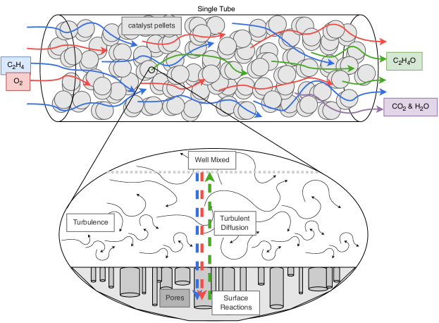
Figure 2: Representation of the catalytic reactor model for ethylene-oxide production. Input gas reactants are passed over a fixed catalytic bed, resulting in production of output products & byproducts, varying in production efficiency. In addition to reaction parameters, the interaction parameters related to catalyst surface and flow turbulence are incorporated.

This model was chosen and constructed to be an extensible problem of a modular system demonstrating properties of complex system models, partitioning the integrated system into various submodels. The reactor is a common industrial process converting feedstocks ethylene and oxygen to ethylene oxide, in a reaction promoted by contact with a solid catalyst packing. The efficiency of the reactor is a function of system controls such as flow rates and temperature and of properties such as reaction rates and catalyst properties.

A brief description of the physical modeling and mathematical solution algorithm for these processes is provided. First, at the largest scale, the complex packing of the pellets into the tube results in an uncertain void fraction, $\varepsilon$. The bulk of the gas flowing through these voids, at a given axial length down the tube, mixes quickly and is then considered to be well approximated by a single chemical composition – this is referred to as the plug-flow approximation. This approach allows a coupled set of steady, one-dimensional differential equations (one equation for each compound) to model the change in chemical composition along the length of the reactor. The coupling among these equations is due to the chemical reaction rate converting the reactant compounds of ethylene and oxygen to either ethylene oxide or carbon dioxide & water vapor. So next at the smallest scales, these reactions occur on the surface of the catalyst and are often limited by the available catalyst area. For this reason, highly porous catalyst pellets are preferred. The diagnostics for the properties of these pores such as the pore diameter, $D$, are trusted but are less than ideal (Osterrieth and et.al.,, 2022). The reaction-rate laws appear mathematically as algebraic expressions that depend on their own parameters, $C_{p1}$ and $K_{e1}$, and present the most probable point of model misspecification (Klugherz and Harriott,, 1971; Pu et al.,, 2019). This submodel for the reaction rate depends on the local chemical composition and is thus calculated separately at each discretized point along the length of the reactor. Finally at the intermediate scales, the amount of reactants at the surface is continually depleted by the reaction which also results in an increased concentration of products at the surface, which must diffuse to the bulk – all resulting in a chemical composition local to the catalyst surface that may differ significantly from the composition in the neighboring bulk. Hence, the intermediate physical processes of pore reaction & diffusion as well as turbulent diffusion in the millimeter-scale layer surrounding the pellet must both be modeled (Koning,, 2002). The additional submodel for the turbulence around the pellet introduces two empirical parameters of $c$ and $n$. Unfortunately, the coupling of these submodels from the bulk to the surface requires an iterative multivariable algebraic solve at each discretized point along the reactor – resulting in a significant increase of computational time. The code for simulating this full model is implemented as a Python package that we utilized for demonstrating cut-Bayesian inference and is available at reference  Smith, (2023).

4.1 Calibration and Cut Parameters

The parameters of the ethylene-oxide production reactor can be grouped by the various submodels included in Figure 1. For the purposes of this example, we first performed a Sobol sensitivity analysis (Sobol,, 2001) in order to select a set of parameters for which ethylene-oxide production is most sensitive. Based on this analysis and the availability of experimental data to calibrate submodels, we chose to focus on the turbulence, reaction rate, and catalyst submodels. The calibration parameters of interest are:

• $c$ and $n$: These parameters describe the relationship between Reynolds number of flow velocity and the turbulent Nusselt number, based on a linear model in a log-log scale.

• $C_{p1}$ and $K_{e1}$: These are reaction rate parameters that determine the rate of ethylene-oxide production, using a rate law provided by Klugherz and Harriott, (1971).

Further, we assume that the cut parameters come from the catalyst submodel, whose distributions are fixed based on domain expertise of catalyst properties:

• $\varepsilon$: Describes the gaps between pellets in the reactor.

• $D$: Diameter of the pores in the reactor.

We used nominal values based on domain expertise for any additional parameter values. Calibration and cut parameters are summarized in the following table. For calibrated parameters, the distribution listed is the prior. For the cut parameters, the distribution is fixed and is not updated.

submodel	parameter	description	distribution
Turbulence	$c$	calibrated	U(.01,3)
	$n$	calibrated	U(-.8,-.05)
Reaction	$C_{p1}$	calibrated	U(0,.1)
	$K_{e1}$	calibrated	U(0,.1)
Catalyst	$D$	cut	U(.019, .021)
	$\varepsilon$	cut	U(.6375, .8625)

Table 1: Parameters used for the reactor model demonstration.

4.2 Model Specification

Experimental data from actual experiments suggested by domain expertise were used for the turbulence and reaction submodels. These data were compiled from many classical experiments that are described and are available in the Python package from Smith, (2023). Let $x_{1},...,x_{M}$ be the univariate turbulence data, $\mathbf{y}_{1},...,\mathbf{y}_{N}$ be the bivariate experimental reaction rate data (one component for ethylene oxide and the second for carbon dioxide), and $z_{1},...,z_{P}$ be the univariate integrated ethylene-oxide production data generated with a high-fidelity model. Placed in a vector, we use the notation $\mathbf{x}$, $\mathbf{y}$, and $\mathbf{z}$. Further, $f_{1}(c,n,i)$ represents the simulator output for the turbulence submodel for the $i$th input setting, $\mathbf{f}_{2}(C_{p1},K_{e1},i)$ represents the simulator output for the reaction rate submodel at the $i$th input setting, and $f_{3}(c,n,C_{p1},K_{e1},\varepsilon,D,i)$ represents the simulator output for the integrated ethylene-oxide production model at the $i$th input setting. Tacitly, the $i$th input setting represents any inputs additional to the parameters that corresponded to the $i$th experimental observation; for instance, Reynolds number for the turbulence model, and temperatures and pressures for the rate kinetics model.

Conditional on the calibration and cut parameter values, we assume that each of the three data sets are independent and observed with independent, 0 mean normal errors with known variances. Estimates of the error variances for each datatype were determined with preliminary simple linear regression fits; we focus in this example solely on the inference of physical parameters. We denote $\sigma^{2}_{1}$ as the variance for the turbulence data, $\Sigma_{2}$ as the 2-by-2 covariance matrix for the reaction rate data, and $\sigma^{2}_{3}$ as the variance for the integrated ethylene-oxide production data.

Thus, we may write the likelihood, conditional on the calibration and cut parameters and simulators, as:

$$p(\mathbf{x},\mathbf{y},\mathbf{z}|c,n,K_{e1},C_{p1},\varepsilon,D)=\\ \prod_{i=1}^{M}\mathcal{N}_{1}(x_{i};f_{1}(c,n,i),\sigma^{2}_{1})\times\prod_{i=1}^{N}\mathcal{N}_{2}(\mathbf{y}_{i};\mathbf{f}_{2}(C_{p1},K_{e1},i),\Sigma_{2})\times\prod_{i=1}^{P}\mathcal{N}_{1}(z_{i};f_{3}(c,n,C_{p1},K_{e1},\varepsilon,D,i),\sigma^{2}_{3}).$$ (7)

The uniform prior distributions for the calibration parameters $c,n,K_{e1}$, and $C_{p1}$ and the uniform cut distributions for $\varepsilon$ and $D$ are specified in Table 1.

4.3 Results

We first implemented an SMC routine based off of Section 2.3 that uses independent draws of the cut parameter. We used 25 particles with 5 slice sampling (Neal,, 2003) mutate steps within the SMC algorithm. We grouped 10 sets of 10 independently drawn cut parameters in a single batch and ran 8 independent batches. To compare the resultant cut-Bayesian posterior samples of $c,n,C_{p1}$, and $K_{e1}$, we generated “gold standard” samples with the direct-sampling method discussed in Section 2. Specifically, conditional on each draw of cut parameters we use the slice-within-Gibbs (Neal,, 2003) algorithm to draw from the conditional posterior of calibration parameters, running for a total of 1000 iterations; 1000 was chosen based on examining traceplots of preliminary runs as well as calculating the Gelman-Rubin convergence diagnostic (Gelman and Rubin,, 1992) using the implementation from the coda package (Plummer et al.,, 2006) for said runs. Pooling all of the calibration samples generated from distinct cut parameter draws results in samples from the cut posterior distribution (Plummer,, 2015). In Figure 3 we see a comparison of cut posterior densities for calibration parameters generated with the SMC method and the direct-sampling method (i.e., using multiple MCMC chains). We see that the densities generally match up, suggesting the SMC method is producing samples of the cut posterior. Appendix B illustrates that pairs plots of samples from the SMC and direct methods show agreement; moreover, the bivariate distributions of pairs indicate curvature that is not characteristic of a bivariate normal distribution. In an effort to further reduce computational runtime, we additionally implemented the linear tempering variant of Section 2.4 with 10 particles and 1 additional point on the line connecting successive cut parameter draws, with 5 independently drawn cut parameters per set. We also reduced the number of mutate steps by 1. The comparison of resultant samples to the the gold standard is given in the density plot of Figure 4, also showing general agreement, and as is next discussed, indicating computational improvement in runtime.

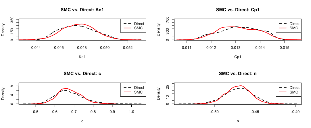
Figure 3: Comparison of SMC cut posterior samples (red density) of calibration parameters to direct-sampling (black density); the densities generally appear to be consistent. Additionally, Appendix B contains a comparison of pairs plots, which show alignment.

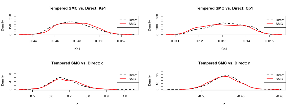
Figure 4: Comparison of tempered SMC cut posterior samples (red density) of calibration parameters to direct-sampling (black density). 10 particles are used for this run in comparison to the 25 used in Figure 3, but with $P=1$, as in Corollary 1. Samples appear to be generally consistent with direct sampling approach but with substantial computational reduction.

Both SMC procedures and the direct-sampling procedure using multiple Markov chains were run on the Los Alamos National Laboratory (LANL) Darwin computing testbed, which is funded by the Computational Systems and Software Environments subprogram of LANL’s Advanced Simulation and Computing program (NNSA/DOE). All methods were batched into 8 jobs where each job was run on its own node on the general partition, but no parallelization was used beyond batching independent runs. Additionally, the BASS R package (Francom and Sansó,, 2020) was used to construct a computationally efficient emulator for the integrated ethylene production model (referred to as $f_{3}$ previously) and the identical emulator was used in the SMC and the direct-sampling procedures. Run time results comparing the SMC method, the linear tempered SMC method, and the direct sampling MCMC method are shown in Table 2, indicating substantial improvement using the SMC methods. The overhead time needed to generate the initial particles required for the SMC methods was 1 hour and 19 minutes.

Method	Min job runtime (minutes)	Max job runtime (minutes)
Direct sampling	645	765
SMC	79	92
Tempered SMC	29	39

Table 2: Comparison of run times in minutes for direct sampling, SMC (Theorem 1), and the linear tempered SMC (Corollary 1).

5 Conclusion and Discussion

Our central contribution is the introduction of SMC methods for computing with cut-Bayesian posteriors. The methods are supported by theoretical results of SMC estimators in fairly general settings as well as finite sample complexity bounds when the conditional posterior is normally distributed, as was motivated by a computer model misspecification problem. Additionally, we have demonstrated the practical utility and accuracy of the methods for cut-Bayes inference with a coupled modular chemical reactor system, and have shown order-of-magnitude computational efficiency gains. To our knowledge, we have presented the first provably correct SMC-based computational method for cut-Bayesian posterior inference. The defining characteristics of our method are that it results in convergent estimators and does not require approximations to conditional distributions. When such approximations are appropriate, alternate methods may be preferred for computational efficiency; however, our SMC method can be used when such approximations cannot be made (see Appendix C for an example in which the conditional posteriors are non-Gaussian). While the unbiased MCMC method of Jacob et al., (2020) could be a viable alternative that does not assume approximations to conditional distributions, care must be taken to ensure that meeting times of coupled Markov chains are not prohibitively expensive, such as when the dimension of the problem increases. The results of Section 3 provide some theoretical guidance for how the complexity of our SMC method scales with dimension for a specific case. A crucial aspect of our theoretical results is that independence is assumed for the cut parameter draws for the application of Hoeffding’s inequality; while concentration results are less prevalent in the case of dependence, future work could explore relaxing the independence assumption in order to derive tighter concentration bounds.

6 Funding Acknowledgment

This work was supported by the U.S. Department of Energy through the Los Alamos National Laboratory. Los Alamos National Laboratory is operated by Triad National Security, LLC, for the National Nuclear Security Administration of U.S. Department of Energy (Contract No. 89233218CNA000001). The authors are grateful for support from the Advanced Simulation and Computing Program’s Verification and Validation subprogram.

Appendix A Proof of Theorem 1

A.1 General Results for SMC Algorithms

We first prove a straightforward extension of the finite sample bounds for SMC algorithms given in Marion et al., (2023). Let $\mu_{0},\ldots,\mu_{S}=\pi$ denote a sequence of distributions defined on a space $\mathcal{X}$ (e.g. $\mathcal{X}=\mathbb{R}^{d}$) with common dominating measure $\rho$. The sequential Monte Carlo algorithm produces a set of particles $\Theta=(\theta^{1:N}_{0},\tilde{\theta}^{1:N}_{1},\theta^{1:N}_{1},\ldots,\tilde{\theta}^{1:N}_{S},\theta_{S}^{1:N})$ jointly defined on $\mathcal{X}^{N(2S+1)}$. The marginal laws of these random variables are implicitly defined by the algorithm given in Section 2.3; we do not state these marginal laws here for brevity but refer the reader to Marion et al., (2023) and Mathews and Schmidler, (2024) for details. In addition, the proof technique of Marion et al., (2023), and the proof technique used here to extend their results, involves constructing a set of random variables denoted $\bar{\theta}^{1:N}_{s}$ via a “maximal” coupling construction at the $s$th step of the algorithm so that $\bar{\theta}^{i}_{s}\sim\mu_{s}$ and $\bar{\theta}^{i}_{s}$ and $\theta^{i}_{s}$ are equal with high probability. The state space we consider throughout is $\mathcal{X}^{N(3S+1)}$ with corresponding product $\sigma$-field $\mathcal{B}^{N(3S+1)}$ corresponding to the particle system $\Theta$ along with the constructed random variables $\bar{\Theta}=(\bar{\theta}^{1:N}_{1},\ldots,\bar{\theta}^{1:N}_{S})$. We let $\operatorname{\mathbb{P}}$ and $\operatorname{\mathbb{E}}$ generically denote the joint probability measure and expectation, respectively, of $\Theta$ and $\bar{\Theta}$ (i.e. the probability space is $(\mathcal{X}^{N(3S+1)},\mathcal{B}^{N(3S+1)},\operatorname{\mathbb{P}})$).

We note that in practice $(\bar{\theta}^{1:N}_{1},\ldots,\bar{\theta}^{1:N}_{S})$ are not constructed during the SMC algorithm; here they are only constructed in theory for the proof technique. We refer the reader to the Appendix of Marion et al., (2023) for details on how the construction of $\bar{\Theta}$ is performed along with some important properties of these random variables. In particular, the authors show that $\bar{\theta}^{i}_{s}\perp\!\!\!\perp\tilde{\theta}^{i}_{s}$ and, consequently, $\bar{\theta}^{1:N}_{s}\overset{iid}{\sim}\mu_{s}$ and

$$\bar{\theta}^{1:N}_{s}\perp\!\!\!\perp(\theta^{1:N}_{0},\theta^{1:N}_{1},\theta^{1:N}_{2},\tilde{\theta}^{1:N}_{2}\bar{\theta}^{1:N}_{2},\ldots,\theta^{1:N}_{s-1},\tilde{\theta}^{1:N}_{s-1}\bar{\theta}^{1:N}_{s-1})$$ (8)

for $s=1,\ldots,S$. We use both of these properties below. As in Marion et al., (2023), let

$$A_{s} =\{\theta^{1:N}_{s}=\bar{\theta}^{1:N}_{s}\}$$

$$B_{s} =\{\bar{w}_{s+1}\geq 2\operatorname{\mathbb{E}}_{\mu_{s}}[w_{s+1}]/3\}$$

$$C_{s} =A_{s}\cap B_{s},$$

where $\bar{\theta}^{1:N}_{0}:=\theta^{1:N}_{0}\overset{iid}{\sim}\mu_{0}$. Marion et al., (2023) show inductively that $\operatorname{\mathbb{P}}(C_{s})$ can be made large for $s=0,\ldots,S$ by choosing $N$ and $t$ sufficiently large. However, here there is no “target” measure and we wish to obtain samples from all distributions $\mu_{0},\ldots,\mu_{S}$. Therefore, we extend this result to show that the joint event $\operatorname{\mathbb{P}}(C_{0}\cap\ldots\cap C_{s})$ holds with high probability. Clearly a bound on $\operatorname{\mathbb{P}}(C_{s})$ implies a bound on this joint probability via the union bound. However, doing so results in a looser bound than what is necessary. Throughout we make the following assumption:

Assumption 3.

There exists $\mathcal{E}>0$ such that

$$\max_{s\in\{1,\ldots,S\}}\chi^{2}(\mu_{s}\mid\mid\mu_{s-1})\leq\mathcal{E}\text{ for }s=1,\ldots,S.$$

We slightly modify the proof given in Marion et al., (2023) to show the following result.

Lemma 1.

Let $\delta\in(0,\frac{1}{4})$ and choose

1. $N\geq 18\log\left(\frac{2(S+1)}{\delta}\right)(\mathcal{E}+1)$

2. $t\geq\max_{s=1,\ldots,S}\tau_{s}(\frac{\delta}{2N(S+1)},2)$

Then for $s\in\{0,\ldots,S\}$:

$$\operatorname{\mathbb{P}}(C_{0},\ldots,C_{s})\geq\left(1-\frac{\delta}{S+1}\right)^{s+1}.$$

The proof of Lemma 1 proceeds by induction and the arguments are near identical to those given in Marion et al., (2023). Consequently, we will often point to results given there. The following lemma establishes the base case.

Lemma 2.

Let $N\geq 18\log\left(\frac{S+1}{\delta}\right)(\mathcal{E}+1)$. Then $\operatorname{\mathbb{P}}(C_{0})\geq 1-\frac{\delta}{S+1}$.

Proof.

Note $\operatorname{\mathbb{P}}(C_{0})=\operatorname{\mathbb{P}}(B_{0})$ since $\bar{\theta}^{1:N}_{0}:=\theta^{1:N}_{0}$. By assumption, $\theta^{1:N}_{0}\overset{iid}{\sim}\mu_{0}$. Hence, by Bernstein’s inequality

$$\operatorname{\mathbb{P}}(B^{c}_{0}) =\operatorname{\mathbb{P}}\left(\frac{1}{N}\sum^{N}_{i=1}w_{1}(\theta^{i}_{0})\leq\frac{2\operatorname{\mathbb{E}}_{\mu_{0}}[w_{1}]}{3}\right)$$

$$\leq\exp\left\{-\frac{N}{18(1+\chi^{2}(\mu_{1}\mid\mid\mu_{0}))}\right\}\leq\frac{\delta}{S+1},$$

where the final inequality follows by our choice of $N$ and Assumption 3. ∎

Proof.

(Lemma 1) The proof proceeds by induction. We use the shorthand notation $\operatorname{\mathbb{P}}(C_{0:s}):=\operatorname{\mathbb{P}}(C_{0},\ldots,C_{s})$ throughout. Lemma 2 establishes the base case by our choice of $N$. Now suppose the claim holds at step $s-1$:

$$\operatorname{\mathbb{P}}(C_{0:s-1})\geq\left(1-\frac{\delta}{S+1}\right)^{s}.$$

Since $\delta\in(0,\frac{1}{4})$, it follows that $\operatorname{\mathbb{P}}(C_{0:s-1})\geq\frac{3}{4}$ by the induction hypothesis. This implies (see Lemma 4.2 of Marion et al., (2023))

$$\operatorname{\mathbb{P}}(\tilde{\theta}^{i}_{s}\in B\mid C_{0:s-1})\leq 2\mu_{s}(B).$$

Consequently, $\mathcal{L}(\tilde{\theta}^{i}_{s}\mid C_{0:s-1})$ is $2$-warm start with respect to $\mu_{s}$, where $\mathcal{L}(\tilde{\theta}^{i}_{s}\mid C_{0:s-1})$ denotes the law of $\tilde{\theta}^{i}_{s}$ conditional on the event $C_{0:s-1}$ occurring. Hence, by a coupling argument (see Lemma 4.1 and the Appendix of Marion et al., (2023)), we can guarantee by our choice of $t$

$$\operatorname{\mathbb{P}}(A_{s}\mid C_{0:s-1})\geq 1-\frac{\delta}{2(S+1)}.$$

Let

$$\bar{B}_{s}=\left\{\frac{1}{N}\sum^{N}_{i=1}w_{s+1}(\bar{\theta}^{i}_{s})\geq 2\operatorname{\mathbb{E}}_{\mu_{s}}[w_{s+1}]/3\right\}.$$

That is, $\bar{B}_{s}$ is the same as $B_{s}$, except we replace the $\theta^{1:N}_{s}$ particles with the constructed “target” random variables $\bar{\theta}^{1:N}_{s}\overset{iid}{\sim}\mu_{s}$. As in the proof of Lemma 2, we have by Bernstein’s inequality and our choice of $N$

$$\operatorname{\mathbb{P}}(\bar{B}^{c}_{s})\leq\frac{\delta}{2(S+1)}.$$

Putting it all together,

$$\operatorname{\mathbb{P}}(C^{c}_{s}\mid C_{0:s-1}) =\operatorname{\mathbb{P}}(B^{c}_{s}\cap A_{s}\mid C_{0:s-1})+\operatorname{\mathbb{P}}(A^{c}_{s}\mid C_{0:s-1})$$

$$\leq\operatorname{\mathbb{P}}(\bar{B}^{c}_{s}\mid C_{0:s-1})+\operatorname{\mathbb{P}}(A^{c}_{s}\mid C_{0:s-1})$$

$$=\operatorname{\mathbb{P}}(\bar{B}^{c}_{s})+\operatorname{\mathbb{P}}(A^{c}_{s}\mid C_{0:s-1})$$

$$\leq\frac{\delta}{S+1}$$

The inequality $\operatorname{\mathbb{P}}(\bar{B}^{c}_{s}\mid C_{1:s-1})=\operatorname{\mathbb{P}}(\bar{B}^{c}_{s})$ follows using (8) (see the Appendix of Marion et al., (2023)). The stated bound follows:

$$\operatorname{\mathbb{P}}(C_{0},\ldots,C_{s})=\operatorname{\mathbb{P}}(C_{s}\mid C_{0},\ldots,C_{s-1})\operatorname{\mathbb{P}}(C_{0},\ldots,C_{s-1})\geq\left(1-\frac{\delta}{S+1}\right)^{s+1}.$$

∎

We now use Lemma 1 to prove Theorem 1. We consider the same probability space as before, except expanded so that $\nu_{0:S}\overset{iid}{\sim}p_{\nu}$ (assumed to also be defined on $\mathcal{X}$) are jointly defined with $\Theta$ and $\bar{\Theta}$; we again let $\operatorname{\mathbb{P}}$ and $\operatorname{\mathbb{E}}$ denote the joint probability measure and expectation, respectively. We appeal to the fact that conditional on $\nu_{0:S}$, the sequence $\mu_{0},\ldots,\mu_{S}$ is fixed and the results above apply.

Proof.

(Theorem 1) We have by our choice of $N$ and $t$ along with Lemma 1 that

$$\operatorname{\mathbb{P}}\left(\theta^{1:N}_{0}=\bar{\theta}^{1:N}_{0},\ldots,\theta^{1:N}_{S}=\bar{\theta}^{1:N}_{S}\mid\max_{s\in\{1,\ldots,S\}}\chi^{2}(\mu_{s}\mid\mid\mu_{s-1})\leq\mathcal{E}_{\alpha}-1\right)\geq 1-\frac{\delta}{3}.$$

By the law of total probability and Assumption 1

$$\operatorname{\mathbb{P}}(\theta^{1:N}_{0}=\bar{\theta}^{1:N}_{0},\ldots,\theta^{1:N}_{S}=\bar{\theta}^{1:N}_{S})\geq 1-\frac{\delta}{3}-\delta_{\alpha}.$$ (9)

Going forward we work with the $(\bar{\theta}^{1:N}_{0},\ldots,\bar{\theta}^{1:N}_{S})$ random variables instead of $(\theta^{1:N}_{0},\ldots,\theta^{1:N}_{S})$ and then appeal to (9) to obtain the stated claim. Let $\mu_{g}(\nu):=\operatorname{\mathbb{E}}_{\pi(\theta\mid\mathbf{y},\nu)}[g(\nu,\theta)]$ denote the mean of $g(\nu,\theta)$ with respect to the distribution $\pi(\theta\mid\mathbf{y},\nu)$ (note $\mu_{g}(\nu)$ is a random variable). Recall that conditional on $\nu_{0},\ldots,\nu_{S}$, the sequence $\mu_{0},\ldots,\mu_{S}$ is fixed and so $\bar{\theta}^{1:N}_{s}\mid\nu_{0:S}\overset{iid}{\sim}\pi(\cdot\mid\mathbf{y},\nu_{s})$ and

$$\operatorname{\mathbb{E}}[g(\nu_{s},\bar{\theta}^{i}_{s})\mid\nu_{0:S}]=\mu_{g}(\nu_{s}),\text{ for }i=1,\ldots,N.$$

By the conditional form of Hoeffding’s inequality (conditional on $\nu_{0:S}$), we have by our choice of $N$ that with probability $1-\frac{\delta}{3}$

$$\left|\frac{1}{N}\sum^{N}_{i=1}g(\nu_{s},\bar{\theta}^{i}_{s})-\mu_{g}(\nu_{s})\right|\leq\frac{\epsilon}{2},\text{ for }s=0,\ldots,S.$$ (10)

Since (10) holds jointly for $s=0,\ldots,S$, this implies that with probability $1-\frac{\delta}{3}$ by the triangle inequality that conditional on $\nu_{0:S},$

$$\left|\frac{1}{S+1}\sum^{S}_{s=0}\left(\frac{1}{N}\sum^{N}_{i=1}g(\nu_{s},\bar{\theta}^{i}_{s})\right)-\frac{1}{S+1}\sum^{S}_{s=0}\mu_{g}(\nu_{s})\right|\leq\frac{\epsilon}{2}.$$ (11)

Recall that $\nu_{0:S}\overset{iid}{\sim}p_{\nu}$ and note that the random variable $|\mu_{g}(\nu_{s})|\leq 1$ since $|g|\leq 1$. Hence, we again have by our choice of $S$ that with probability $1-\frac{\delta}{3}$ (by Hoeffding’s inequality),

$$\left|\frac{1}{S+1}\sum^{S}_{s=0}\mu_{g}(\nu_{s})-\operatorname{\mathbb{E}}_{p_{\nu}}[\mu_{g}(\nu)]\right|\leq\frac{\epsilon}{2}.$$ (12)

By definition, $\operatorname{\mathbb{E}}_{p_{\nu}}[\mu_{g}(\nu)]=\operatorname{\mathbb{E}}_{\pi^{\text{cut}}}[g]$, the expectation under the cut-Bayes posterior. Consequently, (11) and (12) along with the triangle inequality imply that with probability $1-\frac{2\delta}{3}$

$$\left|\frac{1}{S+1}\sum^{S}_{s=0}\left(\frac{1}{N}\sum^{N}_{i=1}g(\nu_{s},\bar{\theta}^{i}_{s})\right)-\operatorname{\mathbb{E}}_{\pi^{\text{cut}}}[g]\right|\leq\epsilon.$$ (13)

Now, (13) holds only for the $(\bar{\theta}^{1:N}_{0},\ldots,\bar{\theta}^{1:N}_{S})$ random variables. However, by appealing to (9) it follows that with probability $1-\frac{\delta}{3}-\delta_{\alpha}$ the same concentration inequalities hold for the $(\theta^{1:N}_{0},\ldots,\theta^{1:N}_{S})$ too. Hence, by (9) and (13) it follows that with probability $1-\delta-\delta_{\alpha}$,

$$\left|\hat{g}-\operatorname{\mathbb{E}}_{\pi^{\text{cut}}}[g]\right|\leq\epsilon.$$

∎

Appendix B Pairs Plots for SMC and Direct Sampling in Reactor Example

Figure 5: SMC cut posterior samples pairs plot versus direct sampling pairs plot for Ke1 pairs.

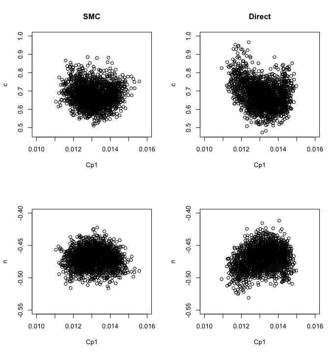
Figure 6: SMC cut posterior samples pairs plot versus direct sampling pairs plot for Cp1 pairs.

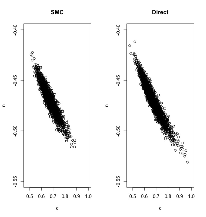
Figure 7: SMC cut posterior samples pairs plot versus direct sampling pairs plot for c,n pair.

Appendix C Non-Gaussian Conditional Posterior

Here we provide a system which illustrates that conditional posteriors in cut Bayesian modeling can be non Gaussian, particularly with nonlinear functions. We consider the calibration parameters $\theta:=(\theta_{1},\theta_{2})\in\mathbb{R}^{2}$ and cut parameter $\nu\in\mathbb{R}^{1}$. The data model $\mathbf{y}|\theta,\nu$ is given by $\mathcal{N}_{2}(f(\theta,\nu),\textrm{diag}(.1,1))$, and uniform, independent priors between $-30$ and $30$ are assumed for the components of $\theta$. Further $f:\mathbb{R}^{3}\rightarrow\mathbb{R}^{2}$ is defined to be:

$$f(\theta_{1},\theta_{2},\nu):=(\sin(\theta_{1})\cos(\theta_{2})\tan(\nu),\theta_{1}^{2}+\theta_{2}^{2}+\nu^{2}).$$

We simulate a single realization of $\mathbf{y}$ according to a true value of $\theta$ equal to (1,2) and $\nu$ equal to 1. The conditional posterior, sampled via slice-within-Gibbs sampling, appears in Figures 8 and 9 below for values of $\nu=1$ and $\nu=.3$ respectively, clearly exhibiting non-Gaussian behavior. This example is meant to illustrate that a normal approximation for the conditional posterior distribution is not always tenable.

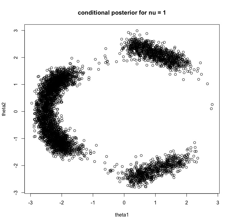
Figure 8: Non-Gaussian conditional posterior for $\nu=1$.

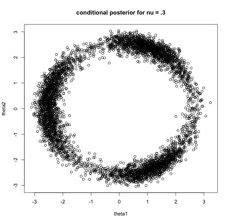
Figure 9: Non-Gaussian conditional posterior for $\nu=.3$.

References

- Baldé et al., (2023) Baldé, O., Damblin, G., Marrel, A., Bouloré, A., and Giraldi, L. (2023). Nonparametric Bayesian approach for quantifying the conditional uncertainty of input parameters in chained numerical models. arXiv preprint arXiv:2307.01111.
- Bayarri et al., (2009) Bayarri, M. J., Berger, J. O., and Liu, F. (2009). Modularization in Bayesian analysis, with emphasis on analysis of computer models. Bayesian Analysis, 4(1):119 – 150.
- Brynjarsdóttir and O’Hagan, (2014) Brynjarsdóttir, J. and O’Hagan, A. (2014). Learning about physical parameters: The importance of model discrepancy. Inverse problems, 30(11):114007.
- Carmona and Nicholls, (2020) Carmona, C. and Nicholls, G. (2020). Semi-modular inference: enhanced learning in multi-modular models by tempering the influence of components. In International Conference on Artificial Intelligence and Statistics, pages 4226–4235. PMLR.
- Carmona and Nicholls, (2022) Carmona, C. U. and Nicholls, G. K. (2022). Scalable semi-modular inference with variational meta-posteriors. arXiv preprint arXiv:2204.00296.
- Chopin, (2004) Chopin, N. (2004). Central limit theorem for sequential Monte Carlo methods and its application to Bayesian inference. Annals of Statistics, 32:2385–2411.
- Del Moral et al., (2012) Del Moral, P., Doucet, A., and Jasra, A. (2012). On adaptive resampling strategies for sequential Monte Carlo methods. Bernoulli, 18(1):252–278.
- Durham and Geweke, (2014) Durham, G. and Geweke, J. (2014). Adaptive sequential posterior simulators for massively parallel computing environments. Bayesian Model Comparison (Advances in Econometrics Vol. 34), pages 1–44.
- Dwivedi et al., (2018) Dwivedi, R., Chen, Y., Wainwright, M., and Yu, B. (2018). Log-concave sampling: Metropolis-Hastings algorithms are fast! Proceedings of the 31st Conference On Learning Theory, 75.
- Francom and Sansó, (2020) Francom, D. and Sansó, B. (2020). BASS: An R Package for Fitting and Performing Sensitivity Analysis of Bayesian Adaptive Spline Surfaces. Journal of Statistical Software, 94(8):1–36.
- Frazier and Nott, (2022) Frazier, D. T. and Nott, D. J. (2022). Cutting feedback and modularized analyses in generalized Bayesian inference. arXiv preprint arXiv:2202.09968.
- Gelman and Rubin, (1992) Gelman, A. and Rubin, D. B. (1992). Inference from iterative simulation using multiple sequences. Statistical Science, 7(4):457–472.
- Higdon et al., (2008) Higdon, D., Gattiker, J., Williams, B., and Rightley, M. (2008). Computer model calibration using high-dimensional output. Journal of the American Statistical Association, 103(482):570–583.
- Hsu et al., (2012) Hsu, D., Kakade, S., and Zhang, T. (2012). A tail inequality for quadratic forms of subGaussian random vectors. Electronic Communications in Probabability.
- Jacob et al., (2017) Jacob, P. E., Murray, L. M., Holmes, C. C., and Robert, C. P. (2017). Better together? Statistical learning in models made of modules. arXiv preprint arXiv:1708.08719.
- Jacob et al., (2020) Jacob, P. E., O’Leary, J., and Atchadé, Y. F. (2020). Unbiased Markov Chain Monte Carlo Methods with Couplings. Journal of the Royal Statistical Society Series B: Statistical Methodology, 82(3):543–600.
- Kennedy and O’Hagan, (2001) Kennedy, M. C. and O’Hagan, A. (2001). Bayesian calibration of computer models. Journal of the Royal Statistical Society: Series B (Statistical Methodology), 63(3):425–464.
- Klugherz and Harriott, (1971) Klugherz, P. D. and Harriott, P. (1971). Kinetics of ethylene oxidation on a supported silver catalyst. AICHE Journal, 17:856–866.
- Koning, (2002) Koning, B. (2002). Heat and Mass Transport in Tubular Packed Bed Reactors at Reacting and Non-Reacting Conditions. PhD thesis, University of Twente.
- Liang et al., (2007) Liang, F., Liu, C., and Carroll, R. J. (2007). Stochastic Approximation in Monte Carlo Computation. Journal of the American Statistical Association, 102(477):305–320.
- Liu and Goudie, (2021) Liu, Y. and Goudie, R. J. B. (2021). Stochastic approximation cut algorithm for inference in modularized Bayesian models. Statistics and Computing, 32(1):7.
- Marion et al., (2023) Marion, J., Mathews, J., and Schmidler, S. C. (2023). Finite-sample complexity of sequential Monte Carlo estimators. The Annals of Statistics, 51(3):1357–1375.
- Mathews and Schmidler, (2024) Mathews, J. and Schmidler, S. C. (2024). Finite sample complexity of sequential Monte Carlo estimators on multimodal target distributions. The Annals of Applied Probability, 34(1B):1199 – 1223.
- Neal, (2003) Neal, R. M. (2003). Slice sampling. The Annals of Statistics, 31(3):705 – 767.
- Osterrieth and et.al., (2022) Osterrieth, J. W. M. and et.al. (2022). How reproducible are surface areas calculated from the bet equation? Advanced Materials, 34(27):2201502.
- Paulin et al., (2019) Paulin, D., Jasra, A., and Thiery, A. (2019). Error bounds for sequential Monte Carlo samplers for multimodal distributions. Bernoulli, 25(1):310–340.
- Plummer, (2015) Plummer, M. (2015). Cuts in Bayesian graphical models. Statistics and Computing, 25:37–43.
- Plummer et al., (2006) Plummer, M., Best, N., Cowles, K., Vines, K., et al. (2006). CODA: convergence diagnosis and output analysis for MCMC. R news, 6(1):7–11.
- Pu et al., (2019) Pu, T., Tian, H., Ford, M. E., Rangarajan, S., and Wachs, I. E. (2019). Overview of selective oxidation of ethylene to ethylene oxide by ag catalysts. ACS Catalysis, 9(12):10727–10750.
- Smith, (2023) Smith, S. T. (2023). https://github.com/smith-lanl/toyproblem-ethyleneox.
- Sobol, (2001) Sobol, I. M. (2001). Global sensitivity indices for nonlinear mathematical models and their monte carlo estimates. Mathematics and computers in simulation, 55(1-3):271–280.
- Stuart and Teckentrup, (2018) Stuart, A. M. and Teckentrup, A. L. (2018). Posterior consistency for Gaussian process approximations of Bayesian posterior distributions. Mathematics of Computation, 87(310):721–753.
- Vempala, (2005) Vempala, S. (2005). Geometric random walks: A survey. Combinatorial and Computational Geometry.
- Wu et al., (2022) Wu, K., Schmidler, S., and Chen, Y. (2022). Minimax mixing time of the Metropolis-adjusted Langevin algorithm for log-concave sampling. Journal of Machine Learning Research, 23:1–63.
- Yu et al., (2021) Yu, X., Nott, D. J., and Smith, M. S. (2021). Variational inference for cutting feedback in misspecified models. arXiv preprint arXiv:2108.11066.