Exploring non-radial oscillation modes in dark matter admixed neutron stars

Abstract

Because of their extreme densities and consequently, gravitational potential, compact objects such as neutron stars can prove to be excellent captors of dark matter particles. Considering purely gravitational interactions between dark and hadronic matter, we construct dark matter admixed stars composed of two-fluid matter subject to current astrophysical constraints of maximum mass and tidal deformability. We choose a wide range of parameters to construct the dark matter equation of state, and the DDME2 parameterization for the hadronic equation of state. We then examine the effect of dark matter on the stellar structure, tidal deformability and non-radial modes considering the relativistic Cowling approximation. We find the effect on $p$-modes is substantial, with frequencies decreasing up to the typical $f-$mode frequency range for most stars with a dark matter halo. The effects on the $f-$mode frequency are less extreme. Finally, we find the most probable and $1\sigma$ values of the dark matter parameters used in this study.

1 Introduction

There are indirect evidences from cosmological and astrophysical observations such as rotation curves of individual galaxies, observed galaxy clusters, and anisotropic microwave background that the dominant contribution to the matter in the Universe is in the form of “dark matter” (DM) which interacts very weakly with ordinary matter [1]. The search for direct detection of DM particles is also ongoing in several experiments [2, 3, 4]. One of the most studied models for DM is the weakly interacting massive particles (WIMP) with masses in ranging from the GeV to the TeV scale. The upper bound of WIMPs scattering off the nuclei is estimated to be $\sim 10^{-44}$ cm² from underground direct search experiments such as CDMS [5] and Xenon10 [6]. Despite the tiny value of the scattering cross-section of DM with ordinary matter, the gravitational influence of DM is very significant. However, nearly all properties of DM remain largely unknown. If DM exists, understanding its nature would provide significant advancements in our understanding of beyond standard model physics.

Many cosmological observations such as the core vs cusp problem, the “satellite problem”, and the “too big to fail problem” favor the self-interacting DM model [7, 8]. Self-interacting DM model may be self-annihilating or non-self-annihilating. If they are self-annihilating, after their capture by compact objects, they will annihilate producing heating inside the compact objects [9, 10, 11, 12]. On the other hand if they do not annihilate, they will be accumulated inside the compact objects. Moreover, the most studied model for DM is the WIMP with a mass above $10$ MeV. Hence, the compact star with large number of accreted DM in the core will easily exceed the Schwarzschild limit and consequently collapse. The asymmetric DM is an interesting alternative of the annihilating WIMP paradigm [13, 14, 15, 16, 17, 18, 19, 20, 21, 22, 23, 24, 25, 26, 27, 28, 29, 30, 31].

Because of the gravitational influence of DM, its properties can be constrained from its effect on the formation and evolution of stars [32, 33]. Compact objects, in this sense, are potential candidates to study DM; not only because of immense gravity which increases the possibility of the capture of particulate DM, but also for their high baryonic density, which increases the probability of DM-nucleon scattering [34, 9, 35, 36, 37, 38, 39]. DM admixed compact stars have been explored in several previous works, considering a variety of DM and compact star models [40, 41, 42, 43, 44, 45, 46, 47, 48, 49, 50, 51, 52, 53, 54, 55].

The recently found lower bound in maximum attainable mass of compact stars [56] indicates the appearance of heavier strange and non-strange baryons in the inner core of the baryonic stars. However, the appearance of these degrees of freedom softens the matter at high density regimes which lowers the maximum attainable mass. If by altering the theoretical proposed model for this kind of matter- for example by taking density-dependent interactions among baryons [57, 58, 59], the matter becomes stiff, the maximum limit of tidal deformability can not be fulfilled [60]. However, as will be shown, the presence of DM can significantly alter the stellar structure, and both the lower limit of maximum attainable mass and the upper limit of tidal deformability can be achieved simultaneously. Consequently, the study of DM admixed compact star property which is very important from particle physics as well as from astrophysical aspects.

We have constructed the DM admixed compact star considering only the gravitational interaction of self-interacting but non-self-annihilating DM with ordinary matter as in refs. [61, 62]. Interested readers may refer to [63, 42, 51]. Due to the lack of evidence and proper knowledge of DM interaction with ordinary matter, we avoid such beyond-standard model interactions in the present work. For a compact star, we consider a neutron star (NS) entirely composed of nucleonic matter. We study the effect on the NS properties connected to the recent and upcoming stellar observations considering the scenario in DM admixed NS. Further, in this context, we will discuss the properties of non-radial oscillations for such stars.

There are several quasi-normal modes like the fundamental ($f$)-mode, pressure ($p$)-modes, gravity ($g$)-modes, spacetime ($w$)-mode, etc [64, 65, 66], each classified based on the restoring forces which work bring the star to equilibrium. For example, the $f-$ and $p_{1}-$ (with on 1 node) modes, which are acoustic waves in the star, are restored by fluid pressure while $g-$modes which arise due to density discontinuities or temperature and composition variations are restored by gravity (buoyancy). Several of these modes can be excited during supernovae explosions or in an isolated perturbed compact star as in the post-merger phase of binary compact stars [67, 68, 69]. Even during the inspiral phase of compact stars, the $f-$mode may be excited [70]. Quadrupolar oscillations ($l=2$) of all modes couple to gravitational waves. With the advent of enhanced next-generation telescopes like the Cosmic Explorer and the Einstein telescope which carry about 10 times the sensitivity of Advanced LIGO, the possibility of detection of these modes increase [67].

2 Hadronic matter model

The model for hadronic matter we discussed here, we assume that normal matter is purely nucleonic and composed of protons, neutrons, and electrons. We consider the relativistic mean field model for ordinary hadronic matter (HM) where the interaction between these nucleons is carried by isoscalar-scalar $\sigma$, isoscalar-vector $\omega$, and isovector-vector $\rho$ mesons along with density-dependent interaction. The Lagrangian density for HM is given as [71]

$$\mathcal{L}_{HM} =\sum_{N}\bar{\psi}_{N}(i\gamma_{\mu}D^{\mu}-m^{*}_{N})\psi_{N}+\frac{1}{2}(\partial_{\mu}\sigma\partial^{\mu}\sigma-m_{\sigma}^{2}\sigma^{2})-\frac{1}{4}\omega_{\mu\nu}\omega^{\mu\nu}+\frac{1}{2}m_{\omega}^{2}\omega_{\mu}\omega^{\mu}-\frac{1}{4}\bm{\rho}_{\mu\nu}\cdot\bm{\rho}^{\mu\nu}$$ (1)

$$+\frac{1}{2}{m_{\rho}^{2}}\bm{{\rho}_{\mu}}\cdot\bm{{\rho}^{\mu}}.$$

Here $N$ denotes nucleons and covariant derivative $D_{\mu}=\partial_{\mu}+ig_{\omega N}\omega_{\mu}+ig_{\rho N}\bm{\tau}_{N3}\cdot\bm{\rho}_{\mu}$. $\psi$ is the nucleonic wavefunction, $\sigma$ the $\sigma$-meson, $\omega_{\mu}$ the $\omega$-meson and $\rho_{\mu}$ the $\rho$-meson fields. The effective nucleon mass is ${{m_{N}}^{*}}={m_{N}}-g_{\sigma{N}}\sigma$. The antisymmetric field terms due to vector meson fields are given by $\omega_{\mu\nu}=\partial_{\mu}\omega_{\nu}-\partial_{\nu}\omega_{\mu}$ and $\bm{\rho}_{\mu\nu}=\partial_{\mu}\bm{\rho}_{\nu}-\partial_{\nu}\bm{\rho}_{\mu}$. The isoscalar meson-nucleon couplings vary with density as

$$g_{iN}(n)=g_{iN}(n_{0})f_{i}(x)\quad\quad\text{for }i=\sigma,\omega$$ (2)

where the function is given by

$$f_{i}(x)=a_{i}\frac{1+b_{i}(x+d_{i})^{2}}{1+c_{i}(x+d_{i})^{2}}$$ (3)

with $x=n/n_{0}$ and $a_{i}$, $b_{i}$, $c_{i}$, $d_{i}$ the parameters which describe the density-dependent nature of the coupling parameters. The isovector-vector $\rho$-meson coupling with nucleons is given by $g_{\rho N}(n)=g_{\rho N}(n_{0})e^{-a_{\rho}(x-1)}$.

With this model the energy density $\varepsilon$ and pressure $p$ of hadronic matter are given by

$$\begin{aligned} \varepsilon_{HM}&=\frac{1}{2}m_{\sigma}^{2}\sigma^{2}+\frac{1}{2}m_{\omega}^{2}\omega_{0}^{2}+\frac{1}{2}m_{\rho}^{2}\rho_{03}^{2}+\sum_{N}\frac{1}{\pi^{2}}\left[p_{{F}_{N}}E^{3}_{F_{N}}-\frac{m_{N}^{*2}}{8}\left(p_{{F}_{N}}E_{F_{N}}+m_{N}^{*2}\ln\left(\frac{p_{{F}_{N}}+E_{F_{N}}}{m_{N}^{*}}\right)\right)\right]\\ &+\frac{1}{\pi^{2}}\sum_{l}\left[p_{{F}_{l}}E^{3}_{F_{l}}-\frac{m_{l}^{2}}{8}\left(p_{{F}_{l}}E_{F_{l}}+m_{l}^{2}\ln\left(\frac{p_{{F}_{l}}+E_{F_{l}}}{m_{l}}\right)\right)\right]\end{aligned}$$ (4)

and,

$$\begin{aligned} p_{HM}&=-\frac{1}{2}m_{\sigma}^{2}\sigma^{2}+\frac{1}{2}m_{\omega}^{2}\omega_{0}^{2}+\frac{1}{2}m_{\rho}^{2}\rho_{03}^{2}+\sum_{N}\frac{1}{12\pi^{2}}\left[p_{{F}_{N}}E^{3}_{F_{N}}-\frac{m_{N}^{*2}}{2}\left(5p_{{F}_{N}}E_{F_{N}}-3m_{N}^{*2}\ln\left(\frac{p_{{F}_{N}}+E_{F_{N}}}{m_{N}^{*}}\right)\right)\right]\\ &+\frac{1}{12\pi^{2}}\sum_{l}\left[p_{{F}_{l}}E^{3}_{F_{l}}-\frac{m_{l}^{2}}{2}\left(5p_{{F}_{l}}E_{F_{l}}-3m_{l}^{2}\ln\left(\frac{p_{{F}_{l}}+E_{F_{l}}}{m_{l}}\right)\right)\right]+n\Sigma^{r}\end{aligned}$$ (5)

respectively with $p_{F_{j}}$, $E_{F_{j}}$ denoting the Fermi momentum and Fermi energy of the $j-$th fermion in the system. Here the rearrangement term $\Sigma^{r}$ arises due to the density dependence of coupling parameters (to maintain thermodynamic consistency) and is given by [72]

$$\Sigma^{r} =\sum_{N}\left[\frac{\partial g_{\omega N}}{\partial n}\omega_{0}n_{N}-\frac{\partial g_{\sigma N}}{\partial n}\sigma n_{N}^{s}+\frac{\partial g_{\rho N}}{\partial n}\rho_{03}\bm{\tau}_{N3}n_{N}\right].$$ (6)

3 Dark matter model

Because of the unclear picture of the DM mass and interactions, theoretically many models of the DM are there that can be incorporated into viable beyond standard model theories. This matter can be fermionic or bosonic, self-interacting via attractive or repulsive potential or even non-interacting [7]. Following previous works [62, 54], we construct the DM model in the relativistic mean-field approach, considering ‘dark’ hadrons that self-interact via ‘dark scalar’ and ‘dark vector’ bosons. We consider fermionic DM with cases of no self-interactions, either scalar or vector self-interactions, or both. DM is assumed to interact with HM only gravitationally. The Lagrangian of DM is given by [62]:

$$\mathcal{L}_{DM}= \bar{\psi_{D}}\quantity[\gamma_{\mu}\quantity(i\partial^{\mu}-g_{vd}V^{\mu})-\quantity(m_{D}-g_{sd}\phi_{D})]\psi_{D}+\frac{1}{2}\quantity(\partial_{\mu}\phi_{D}\partial^{\mu}\phi_{D}-m_{sd}^{2}\phi_{D}^{2})$$

$$-\frac{1}{4}V_{\mu\nu,D}V^{\mu\nu}_{D}+\frac{1}{2}m_{vd}^{2}V_{\mu,D}V^{\mu}_{D}$$ (7)

Here $\psi_{D}$, $\phi_{D}$, and $V^{\mu}_{D}$ represent the fermionic DM, ‘dark scalar meson’, and ‘dark vector meson’ respectively. $m_{D}$ is the bare mass of the fermionic DM. $m_{sd}$ and $m_{vd}$ are the corresponding masses of the scalar and vector ‘dark mesons’ respectively. $g_{sd}$ and $g_{vd}$ are the corresponding coupling strengths. From this Lagrangian, the pressure, energy density, and number density of DM can be given as [62, 52, 54, 51, 73]

$$\varepsilon_{DM}=\frac{1}{\pi^{2}}\left[k_{{F}_{D}}E^{3}_{F_{D}}-\frac{m_{D}^{*2}}{8}\left\{k_{{F}_{D}}E_{F_{D}}+m_{D}^{*2}\ln\left(\frac{k_{{F}_{D}}+E_{F_{D}}}{m_{D}^{*}}\right)\right\}\right]+\frac{n_{DM}^{2}c_{v}^{2}}{2}+\frac{m_{sd}^{2}\phi_{D_{0}}^{2}}{2},$$ (8)

$$p_{DM} =\frac{1}{12\pi^{2}}\left[k_{{F}_{D}}E^{3}_{F_{D}}-\frac{m_{D}^{*2}}{2}\left\{5k_{{F}_{D}}E_{F_{D}}-3m_{D}^{*2}\ln\left(\frac{k_{{F}_{D}}+E_{F_{D}}}{m_{D}^{*}}\right)\right\}\right]+\frac{n_{DM}^{2}c_{v}^{2}}{2}-\frac{m_{sd}^{2}\phi_{D_{0}}^{2}}{2},$$ (9)

$$n_{DM}=\frac{k_{F_{D}}^{3}}{3\pi^{2}}$$ (10)

where $k_{F_{D}}$ is Fermi momentum of DM particle and $E_{F_{D}}=\sqrt{k_{F_{D}}^{2}+m_{D}^{*2}}$ its Fermi energy. $m_{D}^{*}$ is the effective DM fermion mass, given by

$$m_{D}^{*}=m_{D}-g_{sd}\phi_{D_{0}}$$ (11)

and $\phi_{D_{0}}$ is [73]

$$\phi_{D_{0}}=\frac{g_{sd}}{m_{sd}^{2}}\langle\bar{\psi}_{D}\psi_{D}\rangle=\frac{c_{s}^{2}}{g_{sd}}\times\frac{{m_{D}^{*}}}{2\pi^{2}}\quantity[k_{F_{D}}E_{F_{D}}-{m^{*2}_{D}}\ln\left(\frac{k_{{F}_{D}}+E_{F_{D}}}{m_{D}^{*}}\right)]$$ (12)

where $c_{v}=g_{vd}/m_{vd}$ and $c_{s}=g_{sd}/m_{sd}$ are the scalar and vector free parameters.

3.1 DM parameters

In this work, we construct DM EOSs by varying several free parameters- the free DM particle mass, $m_{D}$, the scalar and vector free parameters, $c_{s}$, and $c_{v}$. Since these parameters can take on arbitrary values, we limit them as follows:

• $m_{D}$ is taken in the range of $0.2-2.0$ GeV in intervals of $0.1$ GeV. This range of DM particle masses is arbitrary, but gives pure DM stars with mass in the order of solar mass [53, 74].

• Ranges of $c_{s}$ and $c_{v}$ are arbitrary. Although [62] explores $c_{s}$ and $c_{v}$ in the ranges of $1-7$ $\mathrm{GeV}^{-1}$ and $10-14$ $\mathrm{GeV}^{-1}$ respectively, we vary both of them from $0-50$ $\mathrm{GeV}^{-1}$ in steps of $2$ $\mathrm{GeV}^{-1}$.

• Not all combinations of $c_{s}$, $c_{v}$ and $m_{D}$ give valid EOSs. We discard EOSs where the ${\mathrm{d}p}/{\mathrm{d}\varepsilon}$ becomes negative, or where pressure itself becomes negative.

• As will be explained in section 4.3, to get a stellar model for a DM EOS, we need to fix another parameter- the total DM mass fraction, $M_{f}$. This is the ratio of the mass of DM in a star to the total mass of the star. We vary this parameter from $1\%-20\%$ in steps of $1\%$

4 Stellar Structure and Tidal Deformability

4.1 TOV equations

In our model, DM interacts with HM of the star only via gravitational interaction. Hence, the stellar structure of DM admixed NSs will be governed by the two-fluid stellar structure equations. The two fluids in our case are the HM and the DM. The equilibrium configurations of non-rotating relativistic stars are obtained by solving the Tolmann-Oppenheimer-Volkoff (TOV) equations with the spherically symmetric line element

$$ds^{2}=-\mathrm{e}^{2\Phi}\ dt^{2}+\mathrm{e}^{2\Lambda}\ dr^{2}+r^{2}\ d\theta^{2}+r^{2}\sin^{2}\theta\ d\phi^{2}$$ (13)

The single fluid TOV equations are

$$\frac{\differential m}{\differential r} =4\pi r^{2}\varepsilon$$ (14)

$$\frac{\differential\Phi}{\differential r} =\frac{m+4\pi r^{3}p}{r(r-2m)}$$

$$\frac{\differential p}{\differential r} =-(p+\varepsilon)\frac{\differential\Phi}{\differential r}$$

$$\Lambda(r) =-\frac{1}{2}\ln\quantity(1-\frac{2m}{r})$$

where $m$ is the mass enclosed by the radius $r$, $\Phi$ and $\Lambda$ are the metric functions, $p$ and $\varepsilon$ are the pressure and energy density respectively.

In the two-fluid model the TOV equations become [62]

$$\frac{\differential m_{1}}{\differential r} =4\pi r^{2}\varepsilon_{1}$$ (15)

$$\frac{\differential m_{2}}{\differential r} =4\pi r^{2}\varepsilon_{2}$$

$$\frac{\differential\Phi}{\differential r} =\frac{(m_{1}+m_{2})+4\pi r^{3}(p_{1}+p_{2})}{r(r-2(m_{1}+m_{2}))}$$

$$\frac{\differential p_{1}}{\differential r} =-(p_{1}+\varepsilon_{1})\frac{\differential\Phi}{\differential r}$$

$$\frac{\differential p_{2}}{\differential r} =-(p_{2}+\varepsilon_{2})\frac{\differential\Phi}{\differential r}$$

$$\Lambda(r) =-\frac{1}{2}\ln\left\{1-\frac{2(m_{1}+m_{2})}{r}\right\}$$

These are now five coupled differential equations that need to be solved simultaneously, where the subscripts $1,2$ label the two fluids. At some point during the integration of these equations, the pressure of one of the fluids will vanish, marking the radius $R_{i}$ of fluid $i$. The integration is then switched to solve the single fluid-structure equations 14. When the pressure of the remaining fluid vanishes, we get the final stellar structure. We get the total mass of the star as the sum of the masses of the two fluids. When the radius of the DM is less than that of the other fluid, the star has a DM core, while if the radius is greater, the star has a DM halo surrounding it.

4.2 Dimensionless tidal deformability

A compact star in a binary experiences deformation due to the external quadrupolar field of the companion. Tidal deformability parameter is the measure of the response in terms of the deformability of the star to the external quadrupolar field and defined as the ratio of the induced mass quadrupole moment $Q$ to external perturbing tidal field $\cal{E}$ as [75, 53]

$$\lambda=-\frac{Q}{\cal{E}}=\frac{2}{3}k_{2}R^{5}$$ (16)

where

$$k_{2}={} \frac{8}{5}C^{5}(1-2C^{2})\quantity[2-y_{R}+2C(y_{R}-1)]\times\left\{2C(6-3y_{R}+3C(5y_{R}-8))\right.$$

$$+4C^{3}\quantity[13-11y_{R}+C(3y_{R}-2)+2C^{2}(1+yR)]$$

$$\left.+3(1-2C^{2})\quantity[2-y_{R}+2C(y_{R}-1)]\ln(1-2C)\right\}^{-1}.$$ (17)

$C=M/R$ is the compactness parameter with $M$ and $R$ being the mass and radius of the star respectively. Here $y$ is the solution to the differential equation

$$y^{\prime}=-\frac{1}{r}\quantity(y^{2}+ye^{2\Lambda}\quantity(1+4\pi r^{2}(p-\varepsilon))+Qr^{2})$$ (18)

where

$$Q=4\pi e^{2\Lambda}\quantity(5\varepsilon+9p+(p+\varepsilon)\derivative{\varepsilon}{p})-\frac{6e^{2\Lambda}}{r^{2}}-4\Phi^{\prime 2}$$ (19)

and $y_{R}$ is the value of $y$ at the surface of the star. From here, the dimensionless tidal deformability is defined as

$$\Lambda=\frac{\lambda}{M^{5}}=\frac{2}{3}\frac{k_{2}}{C^{5}}$$ (20)

For two-fluid, DM admixed stars, the modifications in these equations are [62]:

$$\varepsilon\to\varepsilon_{1}+\varepsilon_{2}\qquad p\to p_{1}+p_{2}\qquad(p+\varepsilon)\derivative{\varepsilon}{p}\to(p_{1}+\varepsilon_{1})\derivative{\varepsilon_{1}}{p_{1}}+(p_{2}+\varepsilon_{2})\derivative{\varepsilon_{2}}{p_{2}}$$ (21)

4.3 Dependence on DM parameters

With this two-fluid model, to get the mass-radius (M-R) relation of the star first we need to fix the DM fraction present in the star. We fix the DM fraction by mass as

$$M_{f}=\frac{M(DM)}{M(DM)+M(HM)}$$ (22)

Here M(DM) represents the total mass of the DM in the star, and M(HM) means the same for HM. We use DDME2 density-dependent parametrization for HM in this work [76]. The mass fraction of DM in a particular star is determined completely by the central energy densities of the HM and DM. Since this fraction cannot be known until the structure equations are solved, we employ a root-finding algorithm to find the DM’s central energy density, which would give the required mass fraction for a given central energy density of HM. As the two matter components do not interact with each other, two different spheres are formed. Depending on the central density and EOS of DM, the NS can have a DM core surrounded by HM, or have a DM halo surrounding an HM star. In the case of the M-R relations, we take the radius of the star to be the observable radius of the star (radius of HM) because the electromagnetic probes used to find the radius of the star cannot detect the DM halo [77]. However, when calculating the tidal deformability, we take the star’s radius to the maximum radius among the radius of HM and DM. This is because the DM halo would have a gravitational influence affecting the spacetime geometry [78].

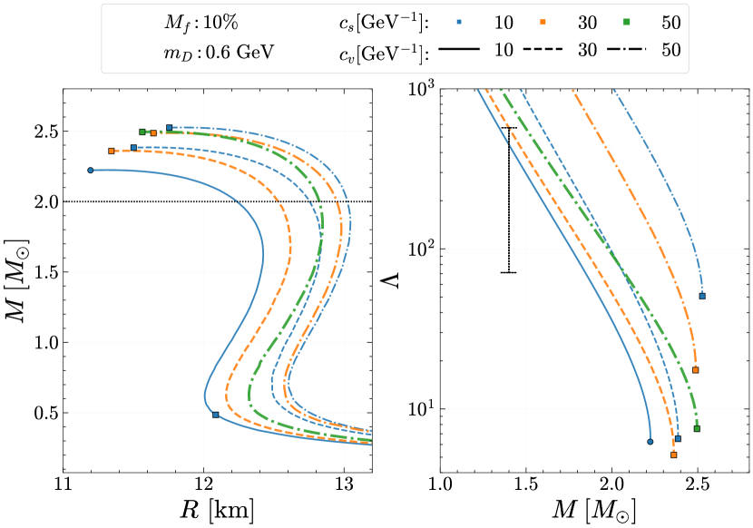
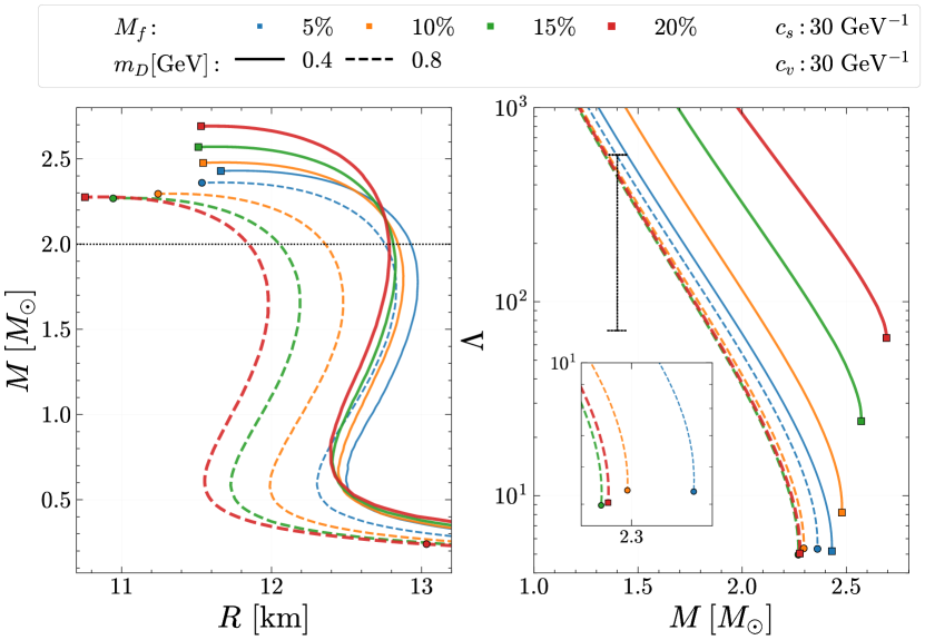
Figure 1: Effects of varying the DM parameters on the $M-R$ (left panel) and $\Lambda-M$ (right panel) relations of DM admixed stars. While decreasing mass, the square marker shows the conversion of DM core to halo and vice versa for the circle marker. The 2$M_{\odot}$ and $\Lambda_{1.4}=190^{+390}_{-120}$ [79] constraints are also shown.

To observe the effects of different parameters on M-R relations and tidal deformability, we choose a few values from the set of parameters as mentioned in section 3.1. For a fixed fraction $M_{f}=10\%$ of DM with particle mass $m_{D}=0.6$ GeV the effect of scalar and vector interactions in the dark sector is shown in the top left panel of figure 1. Here, the square marker shows the transition from DM core to DM halo as mass decreases and vice versa for the transition with the circle marker. For example, for $c_{s}=c_{v}=10\ \mathrm{GeV}^{-1}$, $m_{D}=0.6\ \mathrm{GeV}$ and $M_{f}=10\%$, every star with a mass above the square marker and below the circle marker has a DM core. Keeping the same vector interaction ($c_{v}$), with increasing scalar interaction ($c_{s}$) DM EOS becomes softer. Similarly, keeping $c_{s}$ the same, DM EOS becomes stiffer with an increase of $c_{v}$. Stars having stiffer DM EOS would have DM distributed widely, making them less compact. That is why the DM halo is formed for these stars within the mass range as shown. This less dense DM causes a larger radius of the NS as compared to the NSs having DM cores due to dense DM, this is evident from the left panel of figure 1. In the right panel, we show the variation of $\Lambda$ with mass for different values of $c_{s}$ and $c_{v}$ in the top right panel of figure 1. Again, for stiffer DM EOS the tidal deformability is large as compactness is small. The horizontal dotted line represents the minimum $2~{}M_{\odot}$ maximum mass bound from the M-R relation and the bound on tidal deformability of $1.4~{}M\odot$ star $\Lambda_{1.4}=190^{+390}_{-120}$ [79] is depicted by the vertical dashed line.

For the same scalar and vector interactions, with $c_{s}=c_{v}=30$ GeV^-1 the variation in M-R relation for different $M_{f}$ is shown in the bottom left panel of figure 1 by solid curves for $m_{D}=0.4$ GeV and by dashed curves for $m_{D}=0.8GeV$. Here we observe that for larger $m_{D}$, the DM becomes softer, mostly forming DM cores, and for smaller $m_{D}$ only DM halos are formed for the given combinations. For the softest DM EOS ($c_{s}=c_{v}=30\ \mathrm{GeV}^{-1}$, $m_{D}=0.6\ \mathrm{GeV}$ and $M_{f}=10\%$), we observe the transition from DM core to halo while stellar mass is increasing. In other cases with smaller $M_{f}$ a DM core is formed. In cases of DM halo, to get a larger $M_{f}$, the quantity of DM needs to increase. This increases the maximum mass of the star. In cases of DM core, lesser quantities of HM are needed for greater $M_{f}$. As a result, the maximum mass of the star decreases. This behavior is also evident from the variation of $\Lambda$ which is shown in the bottom right panel of figure 1. We observe that for smaller $m_{D}$ when DM halo is formed, increasing $M_{f}$ decreases the compactness, increasing $\Lambda$; while, for larger $m_{D}$ and cases of DM cores, increasing $M_{f}$ increases compactness, decreasing $\Lambda$. DM halos are more likely to be formed for lower $m_{D}$ and higher $M_{f}$. These conclusions are similar to those obtained by ref. [74].

5 Non Radial Modes

5.1 Equations governing non-radial modes

Due to external or internal perturbations in the star, non-radial oscillations are generated. Here we concentrate on the quadrupolar $l=2$ f- and p1-mode. These modes have pressure as the restoring force and radial node numbers 0 and 1 respectively. We calculate the mode frequencies with the relativistic Cowling approximation. Although the numerical values of frequencies in the Cowling approximation differ from those in the full GR calculations (by up to $30\%$ for $f-$, and $\sim$$15\%$ for $p_{1}-$ [80, 81]), the qualitative results are not affected much.

We follow the formalism given in [82, 83]. Since we’re working within the relativistic Cowling approximation, the metric perturbations are neglected. The fluid perturbations are governed by the fluid Lagrangian displacement vector, which is taken to be

$$\xi^{i}=\quantity(\frac{e^{-\Lambda}}{r^{2}}W(t,r)\ Y_{lm}(\theta,\phi),\ \frac{-V(t,r)}{r^{2}}\ \partial_{\theta}Y_{lm}(\theta,\phi),\ \frac{-V(t,r)}{r^{2}\sin^{2}\theta}\ \partial_{\phi}Y_{lm}(\theta,\phi))$$ (23)

Here $W$ and $V$ are variables of the fluid perturbation. Their relations are obtained by taking a variation of the energy-momentum conservation law $\delta(\nabla_{\nu}T^{\mu\nu})$ which reduces to $\nabla_{\nu}\delta T^{\mu\nu}$ in the Cowling approximation. Here $\delta T^{\mu\nu}$ is given by [83]

$$\delta T^{\mu\nu}=\begin{bmatrix}\ -\delta\varepsilon&\quantity(p+\varepsilon)U^{0}U^{1}&\quantity(p+\varepsilon)U^{0}U^{2}&\quantity(p+\varepsilon)U^{0}U^{3}\ \\[10.0pt] \ \quantity(p+\varepsilon)U^{1}U^{0}&\delta p&0&0\ \\[10.0pt] \ \quantity(p+\varepsilon)U^{2}U^{0}&0&\delta p&0\ \\[10.0pt] \ \quantity(p+\varepsilon)U^{3}U^{0}&0&0&\delta p\ \end{bmatrix}$$ (24)

$U^{\mu}$ is obtained by simply taking a temporal derivative of eq. 23 and noting that the time-like component is the same as that of the unperturbed four velocity for a static perfect fluid in the metric given by eq. 13: ${U}^{0}=e^{-\Phi}$

$$U^{\mu}=\quantity(e^{-\Phi},\ \frac{e^{-\Lambda}}{r^{2}}\partial_{t}W\ Y_{lm},\ \frac{-\partial_{t}V}{r^{2}}\ \partial_{\theta}Y_{lm},\ \frac{-\partial_{t}V}{r^{2}\sin^{2}\theta}\ \partial_{\phi}Y_{lm})$$ (25)

The Eulerian variations of energy density and pressure are given by [83]

$$\delta\varepsilon =\quantity(p+\varepsilon)\frac{\Delta n}{n}-\varepsilon^{\prime}\xi^{r}\qquad\delta p =\gamma p\frac{\Delta n}{n}-p^{\prime}\xi^{r}$$ (26)

where

$$\frac{\Delta n}{n}=-\quantity(e^{-\Lambda}\frac{W^{\prime}}{r^{2}}+\frac{l(l+1)}{r^{2}}V)Y_{lm}$$ (27)

is the lagrangian variation in number density, and

$$\gamma=\partialderivative{\ln p}{\ln n}=\frac{p+\varepsilon}{p}\frac{\partial p}{\partial\varepsilon}$$ (28)

is the adiabatic compressibility index. The dash represents the derivative with respect to $r$.

$W$ and $V$ are assumed to have a harmonic time dependence, i.e., $W(t,r)=W(r)e^{i\omega t}$ and $V(t,r)=V(r)e^{i\omega t}$. We now start framing the perturbation equations following the procedure given in [82]. We substitute the perturbed variables and four-velocity in eq. 24, and take the covariant divergence of the perturbed energy momentum tensor for two free indices $\mu=r,\theta$. Throughout the derivation, we use

$$p^{\prime}=-\Phi^{\prime}(p+\varepsilon)\qquad\text{and}\qquad\frac{p^{\prime}}{p+\varepsilon}=-\Phi^{\prime}$$

both of which are valid in the two-fluid case, with the singular terms replaced by the total ones, since from eqs. 15:

$$p_{1}^{\prime}+p_{2}^{\prime} =-\Phi^{\prime}(p_{1}+\varepsilon_{1}+p_{2}+\varepsilon_{2})=-\Phi^{\prime}(p+\varepsilon)\ \ \text{and,}$$

$$\frac{p_{1}^{\prime}+p_{2}^{\prime}}{p_{1}+\varepsilon_{1}+p_{2}+\varepsilon_{2}} =\frac{-(p_{1}+\varepsilon_{1})\Phi^{\prime}-(p_{2}+\varepsilon_{2})\Phi^{\prime}}{p_{1}+\varepsilon_{1}+p_{2}+\varepsilon_{2}}=-\Phi^{\prime}$$ (29)

To remove the dependence of $\gamma$, we use

$$\frac{p^{\prime}}{\gamma p}=\frac{p^{\prime}}{p+\varepsilon}\ \partialderivative{\varepsilon}{p}\ =-\Phi^{\prime}\ \partialderivative{\varepsilon}{p}$$

which is easily obtained from eq. 28. Making all these substitutions, we finally get:

$$W^{\prime} =\partialderivative{\varepsilon}{p}\quantity[\omega^{2}r^{2}e^{\Lambda-2\Phi}V+\Phi^{\prime}W]-e^{\Lambda}l(l+1)V$$ (30)

$$V^{\prime} =2\Phi^{\prime}V-\frac{e^{\Lambda}}{r^{2}}{W}+\quantity(\derivative{\varepsilon}{p}-\partialderivative{\varepsilon}{p})\quantity[\Phi^{\prime}\ V+\frac{e^{-\Lambda+2\Phi}}{\omega^{2}r^{2}}{\Phi^{\prime 2}}\ W]$$ (31)

These are the oscillation mode equations. As a check of their correctness, note that if we take $\derivative{\varepsilon}{p}=\partialderivative{\varepsilon}{p}$, these equations reduce to those of [82]

$$W^{\prime} =\derivative{\varepsilon}{p}\quantity[\omega^{2}r^{2}e^{\Lambda-2\Phi}V+\Phi^{\prime}W]-e^{\Lambda}l(l+1)V$$ (32)

$$V^{\prime} =2\Phi^{\prime}V-\frac{e^{\Lambda}}{r^{2}}{W}$$

Moreover, for stars with a temperature or composition gradient, these equations are the same as eqs. (25) and (26) of [84] with the transformations $\nu\to 2\Phi$, $\lambda\to 2\Lambda$ for the line element, and

$$\mathbb{W}\to-r^{-(l+1)}W\qquad\text{and}\qquad\mathbb{U}\to r^{-l}e^{-2\Phi}V$$

where $\mathbb{W}$ and $\mathbb{U}$ are the fluid perturbation variables in [84] and $W$ and $V$ are the corresponding variables in this work.

The boundary conditions at the center of the star are $W(r)=Ar^{l+1}$ and $V(r)=-Ar^{l}/l$, where $A$ is an arbitrary constant. The surface boundary condition ($r=R$) is [82] $\Delta p=\gamma p\frac{\Delta n}{n}=0$ which from eq. 27 gives

$$\omega^{2}R^{2}e^{\Lambda(R)-2\Phi(R)}V(R)+\Phi^{\prime}|_{r=R}W(R)=0$$ (33)

In the two-fluid case, the only modification is in the $\derivative{\varepsilon}{p}$ term. Using eq. 29, we get

$$\derivative{\varepsilon}{p} =\derivative{\quantity(\varepsilon_{1}+\varepsilon_{2})}{\quantity(p_{1}+p_{2})}\ =\ \derivative{\varepsilon_{1}}{p_{1}}\frac{p_{1}^{\prime}}{p_{1}^{\prime}+p_{2}^{\prime}}+\derivative{\varepsilon_{2}}{p_{2}}\frac{p_{2}^{\prime}}{p_{1}^{\prime}+p_{2}^{\prime}}$$ (34)

$$\derivative{\varepsilon}{p} =\frac{p_{1}+\varepsilon_{1}}{p_{1}+\varepsilon_{1}+p_{2}+\varepsilon_{2}}\ \derivative{\varepsilon_{1}}{p_{1}}+\frac{p_{2}+\varepsilon_{2}}{p_{1}+\varepsilon_{1}+p_{2}+\varepsilon_{2}}\ \derivative{\varepsilon_{2}}{p_{2}}$$ (35)

Since we don’t consider and temperature or composition gradients, the adiabatic sound speed equal to the equilibrium sound speed. Thus eq. 32, along with the above boundary conditions are the equations used in this work. Once the central energy densities for HM and DM for a particular mass fraction have been identified, we solve the oscillation mode equations to find the frequency $\omega$ subject to boundary conditions. We start with an initial guess for $\omega$ and integrate eq. 32. We then check if that value of $\omega$ satisfies eq. 33. If not, the guess of $\omega$ is improved via the Newton-Raphson algorithm. The lowest root of eq. 32 which satisfies the boundary conditions, $\omega$, is the frequency corresponding to the $f-$mode. The next highest root is the first ($p_{1}-$mode) in a family of pressure modes with ever-increasing frequency and radial node numbers. We check the radial node number to classify the modes by counting the number of times $W$ and $V$ are trivial inside the star.

5.2 Dependence on DM parameters

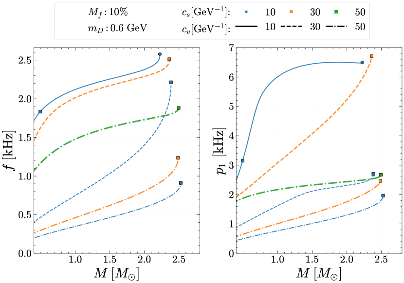
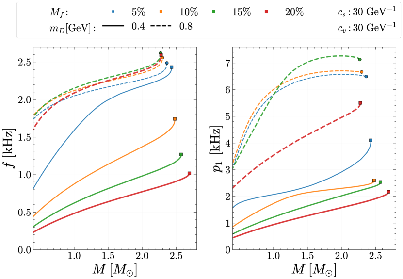
Figure 2: (colors are available in online version) Effects of varying the DM parameters on the $f-M$ (left panel) and $p_{1}-M$ (right panel) relations of DM admixed stars. While decreasing mass, the square marker shows the conversion of DM core to halo and vice versa for the circle marker.

For the same DM parameters as in section 4.3, we see the effects on the non-radial mode frequencies. Figure 2 shows the variation of $f-$ and $p_{1}-$modes frequencies with stellar mass for different parametrizations and $M_{f}$ of DM. As we have seen larger values of $c_{s}$ for a fixed $c_{v}$ make the matter in the star softer, the $f-$ and $p_{1}-$mode frequency increases while larger values of $c_{v}$ for a fixed $c_{s}$ have the opposite effect. This is clear from the top panels of the figure 2. The effect on $p_{1}-$mode frequencies is most notable since the frequencies can decrease a lot, even becoming comparable to the typical ranges of the $f-$mode frequency (1-3 kHz) by suitably varying the DM self-interaction strength.

In the bottom panels of figure 2, we show the variation of non-radial mode frequencies with stellar mass for different $m_{D}$ and $M_{f}$. For both the $f-$ and $p_{1}-$mode cases the variation of frequencies with DM mass fraction is sensitive to whether the star has a DM halo or core. The mode frequencies are less for the DM halo and more for the DM core. When the stars have a DM halo, increasing $M_{f}$ for a fixed $m_{d}$ decreases the mode frequencies as it increases the stiffness, while for stars with DM core, the opposite effect is observed. Again, the effect on the $p_{1}-$mode is much stronger than the effects on the $f-$mode. This is because $p_{1}-$modes, due to the presence of a radial node, are much more sensitive to the distribution of matter in the star [85].

5.3 Correlation studies

We show the mutual dependence of these parameters by the correlations between them in figure 3. Since the effects of DM are heavily dependent on the combinations of the parameters $c_{s}$, $c_{v}$, $m_{D}$, and $M_{f}$, correlations with any one of these parameters is expected to be weak. However as expected, the mode frequencies are strongly correlated with the corresponding compactness. We define compactness as the total mass of the star ($M_{HM}+M_{DM}$) divided by the outermost radius of the star (radius of DM, $R_{DM}$ in case of DM halo, and radius of HM, $R_{HM}$ in case of DM core). The $p_{1}-$modes have a stronger negative correlation with another parameter $\bar{R}=R_{DM}/R_{HM}$ as compared to $f-$modes. This parameter signifies the distribution of DM with respect to HM. This means that the $p_{1}-$mode frequency is more sensitive to the presence of either a DM halo or a DM core than the $f-$mode.

The behavior of the mode frequencies is very similar to that of the tidal deformability as shown in figure 1. When a particular variation of parameters increases the tidal deformability, a decrease in frequency is observed for the same variation. This suggests a negative correlation of the modes with tidal deformability and is indeed what we see in figure 3. Tidal deformability also shows a strong negative correlation with compactness.

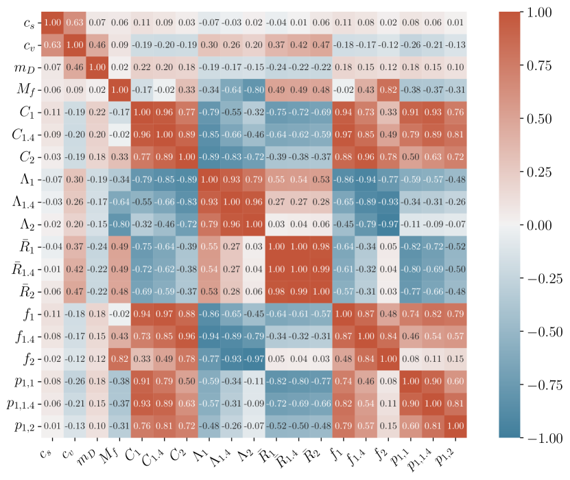
Figure 3: (colors are available in online version) Correlation matrix showing the correlations amongst the DM EOS parameters, stellar structure parameters, and the non-radial modes. Correlations are obtained after applying the minimum 2$M_{\odot}$ maximum mass and $\Lambda_{1.4}=190^{+390}_{-120}$ constraints.

6 DM parameters from astrophysical observations

Next, we constrain the DM parameters for the DM admixed NS from the astrophysical observations of compact objects. We generate M-R relations and tidal deformability with all possible combinations of DM EOS parameters ($c_{s},~{}c_{v},~{}m_{D}$) and $M_{f}$, as mentioned in section 3.1 and then filter our EOSs by making them satisfy the mass constraint of at least 2$M_{\odot}$ maximum mass and the tidal deformability constraint of $\Lambda_{1.4}=190^{+390}_{-120}$. We call DM-admixed stars following these constraints ‘valid’.

Once we have all combinations of parameters that follow these observational constraints, we show a KDE corner plot in figure 5. From the $2,56,880$ total combinations, only $59,030$ combinations give valid DM EOSs with $M-R$ and $\Lambda-M$ curves which follow the observational constraints we impose. We plot probability density plots for the $f-$ and $p_{1}-$modes in figure 4. For this, we first make a $250\times 250$ grid and count the number of lines passing through each grid cell. Upon normalizing, we then have a density map of the $f-M$ and $p_{1}-M$ plane. From this, the $65\%$ (white solid line) and $95\%$ (black dashed line) confidence intervals can be found. We have also shown the $f-$ and $p_{1}-$ modes for DDME2 with no DM as a blue solid line. We find that the $f-$mode frequency for most DM admixed stars takes on a higher value than pure HM. For low mass stars, the $f-$mode frequency decreases a lot, with a minimum of around $1.5\ \mathrm{kHz}$ at $1.4\ M_{\odot}$. However, the change in the $p_{1}-$mode frequency is much more significant. Although the $65\%$ confidence interval encloses the $p_{1}-$mode for pure HM, there is a distinct low-frequency region for the $95\%$ confidence interval. This frequency, between $1-3\ kHz$ is the typical frequency range of $f$-modes. The lowest $p_{1}-$mode frequency at $1.4M_{\odot}$ is around $2.1\ \mathrm{kHz}$. Further, due to the sensitivity of $p_{1}-$modes to the DM distribution, the spread in their frequencies is much larger than that of the $f-$modes. To find the factor responsible for such low frequency $p_{1}-$modes, we utilize a corner plot, in figure 5.

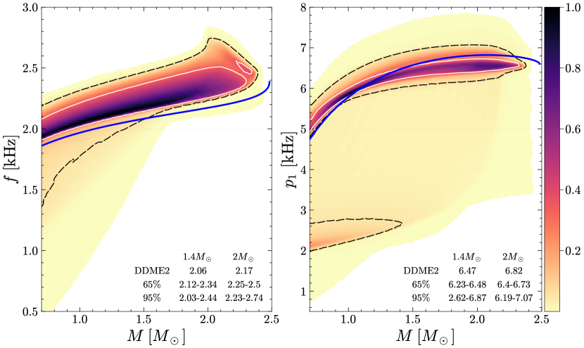
Figure 4: (colors are available in online version) PDFs for $f-M$ (left panel) and $p_{1}-M$ relations for valid stars. The white solid and the black dashed lines represent the $65\%$ and $95\%$ regions respectively. The $f-M$ and $p_{1}-M$ relations for pure HM (DDME2) are shown with a solid blue line. Frequency values given by the confidence intervals at 1.4$M_{\odot}$ and 2$M_{\odot}$ are mentioned along with the frequency values for DDME2 at the same masses.

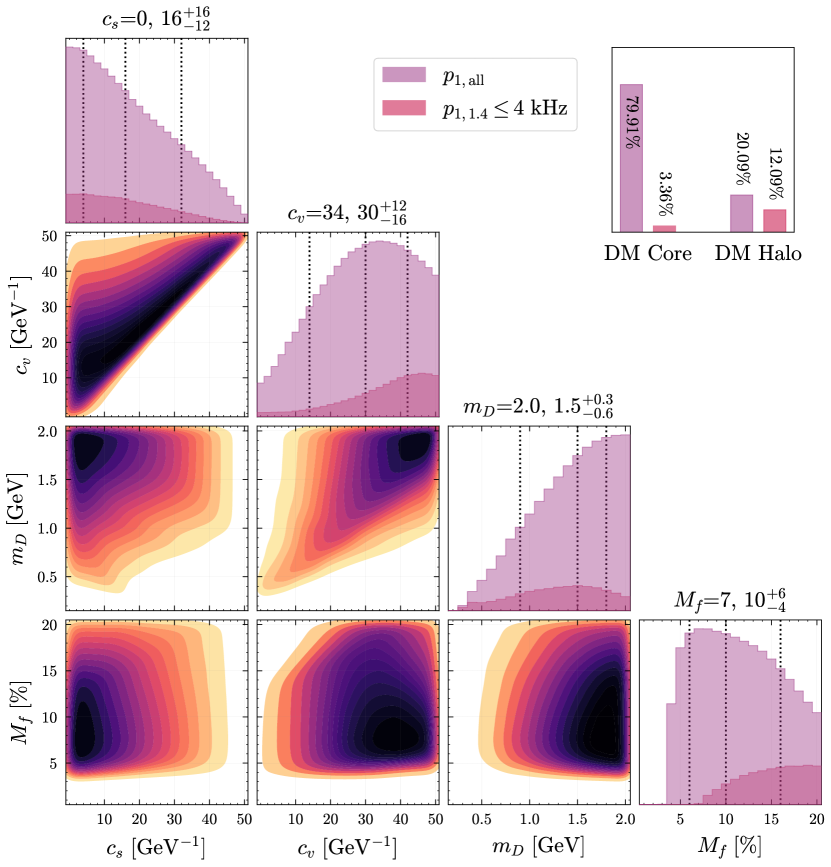
Figure 5: (colors are available in online version) Corner plot with KDEs for the free parameters used in this work. The most probable values of each parameter, along with the median value with $1\sigma$ deviation have been mentioned above the diagonal plots. The bar plot shows the percentage of stars with a DM core or halo. A darker color is used to mark the subset of low-frequency $p_{1}-$modes

We find that the most probable ($1\sigma$) values for or DM parameters are $c_{s}=0\ (4-32)\ \mathrm{GeV}^{-1}$, $c_{v}=34\ (14-42)\ \mathrm{GeV}^{-1}$, $m_{d}=2.0\ (0.9-1.8)\ \mathrm{GeV}$ and $M_{f}=7\ (6-16)\%$. Since increasing $m_{d}$ already reduces the maximum attainable mass and softens the EOS, large $c_{s}$ values are less probable. Large $c_{v}$ values however are more probable since they stiffen the EOS, increasing the maximum mass. Here, it should be noted that the most probable values of the DM parameters depend on the HM EOS chosen. Softer HM EOSs will allow for stiffer DM EOSs, and larger $c_{s}$ values which follow the constraints we imposed. So the range of DM parameters given here is only relevant for DDME2 EOS. Further, since increasing $m_{D}$ softens the DM-admixed star while increasing $c_{v}$ stiffens it, we can get valid DM-admixed stars for very large values of $m_{D}$ and $c_{v}$. As an example, a combination of $c_{s}=0\ \mathrm{GeV}^{-1}$, $c_{v}=50\ \mathrm{GeV}^{-1}$, $m_{D}=50\ \mathrm{GeV}$ and $M_{f}=7\%$ gives a valid star. In this work, we have restricted ourselves to small $m_{D}$ values.

The darker regions in the histogram correspond to the low frequency $p_{1}-$modes. We find that most of our DM-admixed stars have DM cores. However, for stars with DM halo, most of them also have low-frequency $p_{1}-$modes. This means that combinations that are more likely to form a DM halo, i.e. higher $c_{v}$, lower $m_{d}$, and large $M_{f}$ are more likely to give low-frequency $p_{1}-$modes.

7 Summary

We have studied the stellar structure and properties of non-radial oscillation frequencies of DM admixed NSs. We have considered the density-dependent RMF model for the normal HM of the NS and self-interacting but non-annihilating DM which interacts with HM only gravitationally. The DM admixed NS can naturally have a large range of masses and tidal deformabilities since the DM EOS is not constrained. On the other hand, the observed radius of compact objects is related to the extent of HM in the DM admixed NSs. Hence observed M-R relations of the compact objects can be used to constrain the theoretical models of DM admixed NS. Due to their extreme densities, NSs are likely to be excellent captors of particle DM [39]. The properties of DM are not yet established from any theory or experiment. However, if we assume that the astrophysical compact objects contain some fraction of DM, we can estimate some DM properties from astrophysical observations. For example, in our present study, from the observed lower bound of maximum attainable mass of the compact objects and the upper bound of tidal deformability from the binary star merger observations, we predict the maximum probable value of the DM self-interaction parameters and the DM particle mass within a specific model of NS. We also estimate the DM fraction within a DM admixed NS. We find that $7\%$ is the most repeating value of the DM fraction parameter.

The existence of DM admixed NS compels us to study the NS properties which are also important for future GW observations. In light of this, we study the non-radial oscillation frequencies of DM admixed NSs. M-R and tidal deformability constraints help us to filter relevant DM parameters, and we predict the non-radial oscillation frequencies of DM admixed NS with these filtered parameters. We find that the $f-$ and $p_{1}-$mode frequencies are strongly correlated with the compactness and distribution of DM. The $f-$mode frequency increases due to the presence of DM as compared to pure HM stars. But a different trend is observed with the $p_{1}-$mode frequency (typically 4-7 kHz), as the range is more widespread, with frequencies reducing up to the typical range of $f-$mode frequencies (1-3 kHz). A majority of these low frequency $p_{1}-$modes arise in stars with a DM halo, and are more probable in low mass stars. Further, the $p_{1}-$modes for low-mass stars are more sensitive to DM distribution (whether there is a DM core or DM halo) as compared to $f-$modes which is evident from our corner plots and correlation studies. An important conclusion of our paper is thus that the effect of DM capture by compact stars can be seen much more clearly from non-radial modes, especially the $p_{1}-$modes.

Data Availability

The data used in the manuscript can be obtained at reasonable request from the corresponding author.

References

- [1] Gianfranco Bertone, Dan Hooper, and Joseph Silk. Particle dark matter: evidence, candidates and constraints. Phys. Rep., 405(5-6):279–390, January 2005.
- [2] J Aalbers, F Agostini, M Alfonsi, FD Amaro, C Amsler, E Aprile, L Arazi, Francesco Arneodo, P Barrow, L Baudis, et al. Darwin: towards the ultimate dark matter detector. Journal of Cosmology and Astroparticle Physics, 2016(11):017, 2016.
- [3] Rouven Essig, Aaron Manalaysay, Jeremy Mardon, Peter Sorensen, and Tomer Volansky. First direct detection limits on sub-gev dark matter from xenon10. Phys. Rev. Lett., 109:021301, Jul 2012.
- [4] Sergey Alekhin, Wolfgang Altmannshofer, Takehiko Asaka, Brian Batell, Fedor Bezrukov, Kyrylo Bondarenko, Alexey Boyarsky, Ki-Young Choi, Cristóbal Corral, Nathaniel Craig, et al. A facility to search for hidden particles at the cern sps: the ship physics case. Reports on Progress in Physics, 79(12):124201, 2016.
- [5] CDMS II Collaboration, Z. Ahmed, D. S. Akerib, S. Arrenberg, C. N. Bailey, et al. Dark Matter Search Results from the CDMS II Experiment. Science, 327(5973):1619, March 2010.
- [6] J. Angle, E. Aprile, F. Arneodo, L. Baudis, et al. First results from the xenon10 dark matter experiment at the gran sasso national laboratory. Phys. Rev. Lett., 100:021303, Jan 2008.
- [7] Andrea Maselli, Pantelis Pnigouras, Niklas Grønlund Nielsen, Chris Kouvaris, and Kostas D. Kokkotas. Dark stars: Gravitational and electromagnetic observables. Phys. Rev. D, 96(2):023005, July 2017.
- [8] Chris Kouvaris and Niklas Grønlund Nielsen. Asymmetric dark matter stars. Phys. Rev. D, 92(6):063526, September 2015.
- [9] Arnaud de Lavallaz and Malcolm Fairbairn. Neutron stars as dark matter probes. Phys. Rev. D, 81(12):123521, June 2010.
- [10] Nicole F. Bell, Giorgio Busoni, Sandra Robles, and Michael Virgato. Thermalization and annihilation of dark matter in neutron stars. J. Cosmol. Astropart. Phys., 2024(4):006, April 2024.
- [11] Chian-Shu Chen and Yen-Hsun Lin. Reheating neutron stars with the annihilation of self-interacting dark matter. Journal of High Energy Physics, 2018(8):69, August 2018.
- [12] Raghuveer Garani, Aritra Gupta, and Nirmal Raj. Observing the thermalization of dark matter in neutron stars. Phys. Rev. D, 103(4):043019, February 2021.
- [13] S Nussinov. Technocosmology—could a technibaryon excess provide a “natural” missing mass candidate? Physics Letters B, 165(1-3):55–58, 1985.
- [14] S.M. Barr, R. Sekhar Chivukula, and Edward Farhi. Electroweak fermion number violation and the production of stable particles in the early universe. Physics Letters B, 241(3):387–391, 1990.
- [15] Sven Bjarke Gudnason, Chris Kouvaris, and Francesco Sannino. Dark matter from new technicolor theories. Phys. Rev. D, 74(9):095008, November 2006.
- [16] Roshan Foadi, Mads T. Frandsen, and Francesco Sannino. Technicolor dark matter. Phys. Rev. D, 80(3):037702, August 2009.
- [17] Thomas A. Ryttov and Francesco Sannino. Conformal windows of SU(N) gauge theories, higher dimensional representations, and the size of the unparticle world. Phys. Rev. D, 76(10):105004, November 2007.
- [18] Francesco Sannino. Conformal Dynamics for TeV Physics and Cosmology. arXiv e-prints, page arXiv:0911.0931, November 2009.
- [19] Thomas A. Ryttov and Francesco Sannino. Ultraminimal technicolor and its dark matter technicolor interacting massive particles. Phys. Rev. D, 78:115010, Dec 2008.
- [20] Francesco Sannino and Roman Zwicky. Unparticle and higgs boson as composites. Phys. Rev. D, 79:015016, Jan 2009.
- [21] Mads T. Frandsen and Francesco Sannino. Isotriplet technicolor interacting massive particle as dark matter. Phys. Rev. D, 81:097704, May 2010.
- [22] John March-Russell and Matthew McCullough. Asymmetric dark matter via spontaneous co-genesis. J. Cosmol. Astropart. Phys., 2012(3):019, March 2012.
- [23] Mads T. Frandsen, Felix Kahlhoefer, Subir Sarkar, and Kai Schmidt-Hoberg. Direct detection of dark matter in models with a light Z’. Journal of High Energy Physics, 2011:128, September 2011.
- [24] Xin Gao, Zhaofeng Kang, and Tianjun Li. Origins of the isospin violation of dark matter interactions. J. Cosmol. Astropart. Phys., 2013(1):021, January 2013.
- [25] Chiara Arina and Narendra Sahu. Asymmetric inelastic inert doublet dark matter from triplet scalar leptogenesis. Nuclear Physics B, 854(3):666–699, January 2012.
- [26] Matthew R. Buckley and Stefano Profumo. Regenerating a symmetry in asymmetric dark matter. Phys. Rev. Lett., 108:011301, Jan 2012.
- [27] Randy Lewis, Claudio Pica, and Francesco Sannino. Light asymmetric dark matter on the lattice: Su(2) technicolor with two fundamental flavors. Phys. Rev. D, 85:014504, Jan 2012.
- [28] Hooman Davoudiasl, David E. Morrissey, Kris Sigurdson, and Sean Tulin. Baryon destruction by asymmetric dark matter. Phys. Rev. D, 84:096008, Nov 2011.
- [29] Michael L. Graesser, Ian M. Shoemaker, and Luca Vecchi. Asymmetric WIMP dark matter. Journal of High Energy Physics, 2011:110, October 2011.
- [30] Nicole F. Bell, Kalliopi Petraki, Ian M. Shoemaker, and Raymond R. Volkas. Dark and visible matter in a baryon-symmetric universe via the affleck-dine mechanism. Phys. Rev. D, 84:123505, Dec 2011.
- [31] Clifford Cheung and Kathryn M. Zurek. Affleck-dine cogenesis. Phys. Rev. D, 84:035007, Aug 2011.
- [32] Jordi Casanellas and IlíDio Lopes. The Formation and Evolution of Young Low-mass Stars within Halos with High Concentration of Dark Matter Particles. Astro. Phys. J. , 705(1):135–143, November 2009.
- [33] Pat Scott, Malcolm Fairbairn, and Joakim Edsjö. Dark stars at the Galactic Centre - the main sequence. Mon. Not. Roy. Astron. Soc., 394(1):82–104, March 2009.
- [34] Chris Kouvaris. WIMP annihilation and cooling of neutron stars. Phys. Rev. D, 77(2):023006, January 2008.
- [35] Matthew McCullough and Malcolm Fairbairn. Capture of inelastic dark matter in white dwarves. Phys. Rev. D, 81(8):083520, April 2010.
- [36] Chris Kouvaris and Peter Tinyakov. Can neutron stars constrain dark matter? Phys. Rev. D, 82(6):063531, September 2010.
- [37] Richard Brito, Vitor Cardoso, and Hirotada Okawa. Accretion of Dark Matter by Stars. Phys. Rev. Lett., 115(11):111301, September 2015.
- [38] Tolga Güver, Arif Emre Erkoca, Mary Hall Reno, and Ina Sarcevic. On the capture of dark matter by neutron stars. J. Cosmol. Astropart. Phys., 2014(5):013, May 2014.
- [39] Joseph Bramante and Nirmal Raj. Dark matter in compact stars, July 2023.
- [40] Ho-Sang Chan, Ming-chung Chu, Shing-Chi Leung, and Lap-Ming Lin. Delayed Detonation Thermonuclear Supernovae with an Extended Dark Matter Component. Astro. Phys. J. , 914(2):138, June 2021.
- [41] S. C. Leung, M. C. Chu, and L. M. Lin. Dark Matter Admixed Type Ia Supernovae. Astro. Phys. J. , 812(2):110, October 2015.
- [42] Paolo Ciarcelluti and Fredrik Sandin. Have neutron stars a dark matter core? Physics Letters B, 695(1-4):19–21, January 2011.
- [43] S.-C. Leung, M.-C. Chu, and L.-M. Lin. Dark-matter admixed neutron stars. Phys. Rev. D, 84:107301, Nov 2011.
- [44] Z. Rezaei. Study of Dark-matter Admixed Neutron Stars Using the Equation of State from the Rotational Curves of Galaxies. Astro. Phys. J. , 835(1):33, January 2017.
- [45] John Ellis, Gert Hütsi, Kristjan Kannike, Luca Marzola, Martti Raidal, and Ville Vaskonen. Dark matter effects on neutron star properties. Phys. Rev. D, 97:123007, Jun 2018.
- [46] Moira I. Gresham and Kathryn M. Zurek. Asymmetric dark stars and neutron star stability. Phys. Rev. D, 99:083008, Apr 2019.
- [47] Maksym Deliyergiyev, Antonino Del Popolo, Laura Tolos, Morgan Le Delliou, Xiguo Lee, and Fiorella Burgio. Dark compact objects: An extensive overview. Phys. Rev. D, 99:063015, Mar 2019.
- [48] Ann E. Nelson, Sanjay Reddy, and Dake Zhou. Dark halos around neutron stars and gravitational waves. Journal of Cosmology and Astroparticle Physics, 2019(07):012, jul 2019.
- [49] H C Das, Ankit Kumar, Bharat Kumar, S K Biswal, Takashi Nakatsukasa, Ang Li, and S K Patra. Effects of dark matter on the nuclear and neutron star matter. Monthly Notices of the Royal Astronomical Society, 495(4):4893–4903, 05 2020.
- [50] Kilar Zhang, Guo-Zhang Huang, Jie-Shiun Tsao, and Feng-Li Lin. GW170817 and GW190425 as hybrid stars of dark and nuclear matter. European Physical Journal C, 82(4):366, April 2022.
- [51] Ben Kain. Dark matter admixed neutron stars. Phys. Rev. D, 103(4):043009, February 2021.
- [52] Payel Mukhopadhyay and Jürgen Schaffner-Bielich. Quark stars admixed with dark matter. Physical Review D, 93(8):083009, April 2016.
- [53] Kwing-Lam Leung, Ming-chung Chu, and Lap-Ming Lin. Tidal deformability of dark matter admixed neutron stars. Physical Review D, 105(12):123010, June 2022.
- [54] Swarnim Shirke, Suprovo Ghosh, Debarati Chatterjee, Laura Sagunski, and Jürgen Schaffner-Bielich. R-modes as a New Probe of Dark Matter in Neutron Stars, May 2023.
- [55] Swarnim Shirke, Bikram Keshari Pradhan, Debarati Chatterjee, Laura Sagunski, and Jürgen Schaffner-Bielich. Effects of Dark Matter on -mode oscillations of Neutron Stars. arXiv e-prints, page arXiv:2403.18740, March 2024.
- [56] Roger W. Romani, D. Kandel, Alexei V. Filippenko, Thomas G. Brink, and WeiKang Zheng. PSR J0952-0607: The Fastest and Heaviest Known Galactic Neutron Star. Astro. Phys. J. Lett., 934(2):L17, August 2022.
- [57] S. Typel, G. Röpke, T. Klähn, D. Blaschke, and H. H. Wolter. Composition and thermodynamics of nuclear matter with light clusters. Phys. Rev. C, 81(1):015803, January 2010.
- [58] X. Roca-Maza, X. Viñas, M. Centelles, P. Ring, and P. Schuck. Relativistic mean-field interaction with density-dependent meson-nucleon vertices based on microscopical calculations. Phys. Rev. C, 84(5):054309, November 2011.
- [59] A. Taninah, S. E. Agbemava, A. V. Afanasjev, and P. Ring. Parametric correlations in energy density functionals. Physics Letters B, 800:135065, January 2020.
- [60] Vivek Baruah Thapa, Anil Kumar, and Monika Sinha. Baryonic dense matter in view of gravitational-wave observations. Mon. Not. Roy. Astron. Soc., 507(2):2991–3004, October 2021.
- [61] Qian-Fei Xiang, Wei-Zhou Jiang, Dong-Rui Zhang, and Rong-Yao Yang. Effects of fermionic dark matter on properties of neutron stars. Phys. Rev. C, 89(2):025803, February 2014.
- [62] Arpan Das, Tuhin Malik, and Alekha C. Nayak. Dark matter admixed neutron star properties in light of gravitational wave observations: A two fluid approach. Phys. Rev. D, 105:123034, Jun 2022.
- [63] Fredrik Sandin and Paolo Ciarcelluti. Effects of mirror dark matter on neutron stars. Astroparticle Physics, 32(5):278–284, December 2009.
- [64] Kostas D. Kokkotas and Bernd G. Schmidt. Quasi-Normal Modes of Stars and Black Holes. Living Reviews in Relativity, 2(1):2, September 1999.
- [65] Lee Lindblom and Steven L Detweiler. The quadrupole oscillations of neutron stars. Astrophysical Journal Supplement Series (ISSN 0067-0049), vol. 53, Sept. 1983, p. 73-92., 53:73–92, 1983.
- [66] Steven Detweiler and Lee Lindblom. On the nonradial pulsations of general relativistic stellar models. The Astrophysical Journal, 292:12–15, 1985.
- [67] K. D. Kokkotas, T. A. Apostolatos, and N. Andersson. The inverse problem for pulsating neutron stars: a ‘fingerprint analysis’ for the supranuclear equation of state. Mon. Not. Roy. Astron. Soc., 320(3):307–315, January 2001.
- [68] Nikolaos Stergioulas, Andreas Bauswein, Kimon Zagkouris, and Hans-Thomas Janka. Gravitational waves and non-axisymmetric oscillation modes in mergers of compact object binaries. Mon. Not. Roy. Astron. Soc., 418(1):427–436, November 2011.
- [69] Stamatis Vretinaris, Nikolaos Stergioulas, and Andreas Bauswein. Empirical relations for gravitational-wave asteroseismology of binary neutron star mergers. Phys. Rev. D, 101(8):084039, April 2020.
- [70] Cecilia Chirenti, Roman Gold, and M. Coleman Miller. Gravitational Waves from F-modes Excited by the Inspiral of Highly Eccentric Neutron Star Binaries. Astro. Phys. J. , 837(1):67, March 2017.
- [71] Norman K. Glendenning. Compact Stars. 1996.
- [72] Frank Hofmann, C. M. Keil, and H. Lenske. Application of the density dependent hadron field theory to neutron star matter. Phys. Rev. C, 64(2):025804, August 2001.
- [73] Grigoris Panotopoulos and Ilidio Lopes. The dark matter effect on realistic equation of state in neutron stars. Physical Review D, 96(8):083004, October 2017.
- [74] Hong-Ming Liu, Jin-Biao Wei, Zeng-Hua Li, G. F. Burgio, H. C. Das, and H. J. Schulze. Dark matter effects on the properties of neutron stars: compactness and tidal deformability. arXiv e-prints, page arXiv:2403.17024, March 2024.
- [75] Tanja Hinderer. Tidal love numbers of neutron stars. The Astrophysical Journal, 677(2):1216, apr 2008.
- [76] G. A. Lalazissis, T. Nikšić, D. Vretenar, and P. Ring. New relativistic mean-field interaction with density-dependent meson-nucleon couplings. Phys. Rev. C, 71(2):024312, February 2005.
- [77] Davood Rafiei Karkevandi, Soroush Shakeri, Violetta Sagun, and Oleksii Ivanytskyi. Tidal Deformability as a Probe of Dark Matter in Neutron Stars. arXiv e-prints, page arXiv:2112.14231, December 2021.
- [78] D. Rafiei Karkevandi, S. Shakeri, V. Sagun, and O. Ivanytskyi. Tidal deformability as a probe of dark matter in neutron stars. In Remo Ruffino and Gregory Vereshchagin, editors, The Sixteenth Marcel Grossmann Meeting. On Recent Developments in Theoretical and Experimental General Relativity, Astrophysics, and Relativistic Field Theories, pages 3713–3731, July 2023.
- [79] The LIGO Scientific Collaboration and the Virgo Collaboration. Gw170817: Measurements of neutron star radii and equation of state. Phys. Rev. Lett., 121:161101, Oct 2018.
- [80] Athul Kunjipurayil, Tianqi Zhao, Bharat Kumar, Bijay K. Agrawal, and Madappa Prakash. Impact of the equation of state on - and - mode oscillations of neutron stars. Phys. Rev. D, 106:063005, Sep 2022.
- [81] Tianqi Zhao and James M. Lattimer. Universal relations for neutron star -mode and -mode oscillations. Phys. Rev. D, 106:123002, Dec 2022.
- [82] Hajime Sotani, Nobutoshi Yasutake, Toshiki Maruyama, and Toshitaka Tatsumi. Signatures of hadron-quark mixed phase in gravitational waves. Phys. Rev. D, 83:024014, Jan 2011.
- [83] Kip S. Thorne and Alfonso Campolattaro. Non-Radial Pulsation of General-Relativistic Stellar Models. I. Analytic Analysis for L 2. Astrophysical Journal, vol. 149, p.591, September 1967.
- [84] Tianqi Zhao, Constantinos Constantinou, Prashanth Jaikumar, and Madappa Prakash. Quasinormal modes of neutron stars with quarks. Phys. Rev. D, 105:103025, May 2022.
- [85] N. Andersson and K. D. Kokkotas. Towards gravitational wave asteroseismology. Monthly Notices of the Royal Astronomical Society, 299(4):1059–1068, October 1998.