Estimating the Hallucination Rate of Generative AI

Abstract

This work is about estimating the hallucination rate for in-context learning (ICL) with Generative AI. In ICL, a conditional generative model (CGM) is prompted with a dataset and asked to make a prediction based on that dataset. The Bayesian interpretation of ICL assumes that the CGM is calculating a posterior predictive distribution over an unknown Bayesian model of a latent parameter and data. With this perspective, we define a hallucination as a generated prediction that has low-probability under the true latent parameter. We develop a new method that takes an ICL problem—that is, a CGM, a dataset, and a prediction question—and estimates the probability that a CGM will generate a hallucination. Our method only requires generating queries and responses from the model and evaluating its response log probability. We empirically evaluate our method on synthetic regression and natural language ICL tasks using large language models.

1 Introduction

This work is about estimating the hallucination rate for in-context learning (ICL). In ICL, we feed a dataset to a conditional generative model (CGM) and ask it to make a prediction based on that dataset [1, 2]. This practice is useful because it allows us to use pre-trained models to solve problems that they may not have been explicitly optimized for. For example, ICL can improve the prediction accuracy of large language models (LLMs) for benchmark tasks in math, translation, and time series prediction [3, 4]. However, it is difficult to understand the errors a particular ICL application might make—in the terminology of Generative AI, such errors are poetically called hallucinations [5].

We develop a new method that takes an ICL problem—that is, a CGM, a dataset, and a prediction question—and estimates the probability that it will generate a hallucination as a solution. Figure 1(a) shows an ICL problem with news snippets classified as World, Sports, Business, or Science [6], where the last snippet’s correct answer is Sports. Figure 1(b) displays responses generated by Llama-2-7B, with 25% incorrect.

The main idea is to take a Bayesian perspective of ICL, whereby we assume that the CGM is sampling from a posterior predictive distribution over an (unknown) Bayesian model of a latent parameter and data [7, 8]. We can then define the posterior hallucination rate (PHR) under this model, which conditions on the observed data (here, the "context"). Finally, we show how to estimate the posterior hallucination rate using the predictive distribution of a CGM.

Related work. Hallucination prediction and mitigation is an active area of research [9, 10, 11, 12, 13, 14, 15, 16, 17, 18, 19, 20, 21, 22, 23, 24, 25, 26, 27, 28, 29, 30]. This work is most closely related to a subset of methods based on uncertainty quantification [31, 32, 33, 34, 35, 36, 37, 38]. Particularly those methods that aim to predict hallucinations based on uncertainty about the meaning of generated responses [33, 34, 36]. Unlike the latter methods, the PHR does not require external information from auxiliary classifiers and is applicable beyond language tasks. Our approach is enabled by sampling ICL dataset completions from the predictive distribution, which was first explored in the context of sequential models by Fong et al. [39]. Extensions to various CGMs are an active area of research [40, 41]. Notably, Falck et al. [41] studies the hypothesis that ICL performs Bayesian inference. It proposes a method, which is similar to ours, to test that hypothesis, and it presents several ICL problems where the hypothesis does not hold.

Contributions. In Section 2, we introduce the posterior hallucination rate for Bayesian CGMs, prove that the it can be computed by sampling from the predictive distribution, and provide a finite-sample estimator for CGMs that only further requires evaluating the log probabilities of responses. In Section 3, we empirically evaluate our methods. We study the PHR estimator with synthetic data to demonstrate that it can accurately predict the true hallucination rate. We then study our methods on natural language ICL problems with pre-trained CGMs from the Llama-2 family [42] and demonstrate that the PHR estimator can be used to give accurate estimates of the empirical error rate.

Input: This week’s schedule TODAY’S GAMES Division 1 GREATER BOSTON --Arlington at Malden 6:30... Label: Sports Input: Putting Nature on the Pill Wildlife managers are looking to contraception as a way to control... Label: Science Input: Error of Judgment The FBI alleges that a veteran U.S. diplomat met with agents from Taiwan... Label: World Input: Sears and Kmart to Merge After much speculation, two discount giants move to create third... Label: Business Input: Defeat for GB canoeists British canoeists Nick Smith and Stuart Bowman are out of the men’s C2... Label:

(a) An in-context learning dataset.

Sports, Olympics, Other, Sports, Sports, Sports, Sports, Sports, Sports, Sports, Sports, Olympics, Sports, Athletics, Sports, Entertainment, Sports, Sports, Sports, Sports, Olympics, Sports, Sports, Sports

(b) Generated responses

Figure 1: An example of an in-context dataset and generated response examples for the last label. The correct response, "Sports", is given in green and wrong answers are given in purple.

2 The posterior hallucination rate and how to estimate it

In this section, we review the basics of conditional generative models (CGMs). We define in-context learning (ICL) and discuss the Bayesian perspective. We define hallucinations and hallucination rates. Finally, we show how to estimate the hallucination rate given an ICL problem and a CGM.

Conditional generative models and in-context learning.

A conditional generative model (CGM) is a sequential model of the form $p_{\bm{\theta}}(\mathrm{t}\mid(\mathrm{t}_{i})_{1}^{n})$ where $\bm{\theta}$ represents the parameters of the model and $\mathrm{t}_{i}$ are the elements over which the distribution is defined. If the support of each conditional distribution is over linguistic units and the size of $\bm{\theta}$ is large, these models are known as large language models (LLMs). We focus on LLMs, but our methods are applicable to many conditional generative models.

Conditional generative models over sequences are most commonly implemented through sequential neural network architectures called Transformers [43]. The parameters $\bm{\theta}$ are set by performing stochastic maximization of the model likelihood over a training dataset $\mathcal{D}=\{(\mathrm{t}_{i}^{j})_{1}^{n}\}_{j=1}^{m}$, where $i$ is the index over elements of a sequence and $j$ is the index over sequences. The resulting generative model approximates the distribution of sequences of data in the training dataset $\mathcal{D}$.

An in-context learning (ICL) problem is a tuple $(p_{\bm{\theta}},\mathcal{D}_{n},\mathrm{x})$ containing a model $p_{\bm{\theta}}$, a dataset $\mathcal{D}_{n}$, and a query $\mathrm{x}$. The dataset, or "context", is a sequence of ${n}$ examples, $\mathcal{D}_{n}=(\mathrm{x}_{i},\mathrm{y}_{i})_{1}^{n}=((\mathrm{x}_{1},\mathrm{y}_{1}),\dots,(\mathrm{x}_{n},\mathrm{y}_{n}))$. For a new query, $\mathrm{x}$, the model is prompted with the query $\mathrm{x}$ and context $(\mathrm{x}_{i},\mathrm{y}_{i})_{1}^{n}$ to generate a response according to $p_{\bm{\theta}}(\mathrm{y}\mid(\mathrm{x}_{i},\mathrm{y}_{i})_{1}^{n},\mathrm{x})$.

ICL and Bayesian inference. One perspective on ICL connects it to Bayesian statistics [7, 8]. This perspective assumes that there is a joint distribution $p_{\text{ICL}}$ over all sequences of query and response pairs $\mathcal{D}_{n}$. The key idea is that this distribution can be represented as

$$p_{\text{ICL}}(\mathcal{D}_{n})=\int\prod_{i=1}^{n}p_{\text{ICL}}((\mathrm{x}_{i},\mathrm{y}_{i})\mid\mathrm{f})d\mathrm{P}_{\text{ICL}}(\mathrm{f}),$$ (1)

where $\mathrm{f}$ is a latent mechanism that determines which task is being performed. Further, we assume that the pre-trained language model $p_{\bm{\theta}}$ approximates the posterior predictive distribution under $p_{\text{ICL}}$,

$$p_{\bm{\theta}}(\mathrm{y}_{n+1}\mid\mathrm{x}_{n+1},\mathcal{D}_{n}) \approx p_{\text{ICL}}(\mathrm{y}_{n+1}\mid\mathrm{x}_{n+1},\mathcal{D}_{n})$$ (2)

$$=\int p_{\text{ICL}}(\mathrm{y}_{n+1}\mid\mathrm{x}_{n+1},\mathrm{f})d\mathrm{P}_{\text{ICL}}(\mathrm{f}\mid\mathcal{D}_{n}).$$ (3)

Under this assumption, ICL with an LLM is a form of implicit Bayesian inference [8]. Equation 1 is usually justified by de Finetti-style arguments based on exchangeability [44], while Equation 2 must be assumed. We discuss this further in Section B.1.

We now show how adopting this approach will allow us to construct and estimate a posterior hallucination rate: the probability that a generated response $\mathrm{y}$ from $p_{\bm{\theta}}$ to a query $\mathrm{x}$ will be in an unlikely region according to the “true” latent mechanism $\mathrm{f}$.

Before we continue, we establish our notation and terminology thus far. We use the term mechanism to denote a generating process $\mathrm{f}$ belonging to a set $\mathcal{F}$, and let $\mathcal{X}\times\mathcal{Y}$ be a set of query-response pairs $(\mathrm{x},\mathrm{y})$. We use $\mathrm{F},\mathrm{X},\mathrm{Y}$ to denote random variables where appropriate and $\mathrm{f},\mathrm{x},\mathrm{y}$ to denote particular instantiations of these random variables. We assume a distribution $p(\mathrm{f})$ over $\mathcal{F}$ and that $\mathrm{f}$ indexes a set of distributions over query-response pairs, $p(\mathrm{x},\mathrm{y}\mid\mathrm{f})$. These elements allow us to define the joint distribution $p(\mathrm{f},(\mathrm{x}_{i},\mathrm{y}_{i})_{1}^{n})$ and posterior distributions $p(\mathrm{f}\mid(\mathrm{x}_{i},\mathrm{y}_{i})_{1}^{n})$. Moreover, they afford definition of posterior predictive distributions over responses $p(\mathrm{y}\mid(\mathrm{x}_{i},\mathrm{y}_{i})_{1}^{n},\mathrm{x})$, examples $p(\mathrm{x},\mathrm{y}\mid(\mathrm{x}_{i},\mathrm{y}_{i})_{1}^{n})$, and sequences of examples $p(\mathrm{x}_{n+1},\mathrm{y}_{n+1},\dots,\mathrm{x}_{n+k},\mathrm{y}_{n+k}\mid(\mathrm{x}_{i},\mathrm{y}_{i})_{1}^{n})$. We use $\mathcal{D}_{n}$ to denote the dataset of examples $(\mathrm{x}_{i},\mathrm{y}_{i})_{1}^{n}$. For clarity, we use $p_{\bm{\theta}}$ whenever we refer to the distribution of the CGM and $p$ with no subscript when referring to the probability of the “true” generating process. This can be $p_{\text{ICL}}$ or any other probability distribution that follows Equation 1.

2.1 Hallucinations and the posterior hallucination rate

Using the ideas of CGMs and ICL, we now define hallucinations and the hallucination rate.

First, imagine a setting where we observe a true mechanism $\mathrm{f}^{\star}$. For a query $\mathrm{x}$, what values of $\mathrm{y}$ would we consider hallucinations? A simple idea is to call hallucinations those values of $\mathrm{y}$ that are unlikely to be generated from $p(\mathrm{y}\mid\mathrm{x},\mathrm{f}^{\star})$. This motivates the following two definitions.

Definition 1.

We define a (1-${\epsilon}$)–likely set of $\mathbf{\mathrm{f}}$ and $\mathbf{\mathrm{x}}$ as any set $A$ such that $\mathrm{P}(\mathrm{Y}\in A\mid\mathrm{f},\mathrm{x})\geq 1-\epsilon$.

Definition 2.

For fixed (1-$\epsilon$)–likely sets $A(\mathrm{f},\mathrm{x})$, we call a value $\mathrm{y}$ a hallucination with respect to $\mathrm{x}$ and $\mathrm{f}$, if $\mathrm{y}\notin A(\mathrm{x},\mathrm{f})$.

As a simple intuitive example, assume that the true generative model of $(\mathrm{x}_{i},\mathrm{y}_{i})_{1}^{n}$ is a Bayesian linear model with a known standard deviation $\sigma$. Specifically, $\mathrm{F}\sim p(\mathrm{f})$, $\mathrm{X}_{i}\sim\mathcal{N}(0,I_{n})$, and $\mathrm{Y}_{i}\sim\mathcal{N}(\mathrm{F}^{\top}\mathrm{X}_{i},\sigma^{2})$, where $\mathrm{F},\mathrm{X}_{i}\in\mathbb{R}^{d}$ and $\mathrm{Y}_{i}\in\mathbb{R}$. If $\epsilon=0.05$, we could choose the interval between the $2.5$ and $97.5$ percentiles of the distribution $\mathcal{N}(\mathrm{f}^{\star\top}\mathrm{x},\sigma^{2})$ as our (1-$\epsilon$)–likely set and call everything outside of this interval a hallucination.

In practice, we do not observe $\mathrm{f}^{\star}$. Rather, we make predictions with $p(\mathrm{y}\mid\mathrm{x},\mathcal{D}_{n})$. We ask: At what rate are we hallucinating when we make predictions? The answer is the true hallucination rate.

Definition 3.

We define the true hallucination rate (THR), or the probability of sampling a hallucination given true mechanism $\mathrm{f}^{\star}$ and query $\mathrm{x}$ by,

$$h_{\epsilon}^{\star}(\mathrm{f}^{\star},\mathrm{x})\coloneqq\int\mathbbm{1}{\left\{\mathrm{y}\notin A(\mathrm{f}^{\star},\mathrm{x})\right\}}\,d\mathrm{P}(\mathrm{y}\mid\mathcal{D}_{n},\mathrm{x}).$$ (4)

This value is higher when the posterior predictive $p(\mathrm{y}\mid\mathcal{D}_{n},\mathrm{x})$ places high probability in regions unlikely under $p(\mathrm{y}\mid\mathrm{f}^{\star},\mathrm{x})$, or very low if the posterior predictive puts a lot of mass on areas likely under $p(\mathrm{y}\mid\mathrm{f}^{\star},\mathrm{x})$. We expect the value to be higher when we don’t have enough examples and lower as the dataset size increases.

Of course, we do not observe the true mechanism $\mathrm{f}^{\star}$. But the dataset ("context") $\mathcal{D}_{n}$ provides evidence for it, as summarized in the posterior $p(\mathrm{f}\mid\mathcal{D}_{n})$. With this distribution we define the posterior hallucination rate, which is the centerpiece of this work.

Definition 4.

We define the posterior hallucination rate (PHR) as

$$h_{\epsilon}(\mathrm{x})\coloneqq\mathbb{E}\left[h_{\epsilon}^{\star}(\mathrm{F},\mathrm{x})\mid\mathcal{D}_{n}\right]=\iint\mathbbm{1}{\left\{\mathrm{y}\notin A(\mathrm{f},\mathrm{x})\right\}}\,d\mathrm{P}(\mathrm{y}\mid\mathcal{D}_{n},\mathrm{x})\,d\mathrm{P}(\mathrm{f}\mid\mathcal{D}_{n}).$$ (5)

In linear regression, the PHR is the probability that $\mathrm{y}$ will land outside of the high probability interval of $\mathrm{f}$ and $\mathrm{x}$ when sampling $\mathrm{F}\sim p(\mathrm{f}\mid\mathcal{D}_{n})$ and $\mathrm{Y}\sim p(\mathrm{y}\mid\mathcal{D}_{n},\mathrm{x})$.

Here we remind the reader that we still cannot calculate $p(\mathrm{f}\mid\mathcal{D}_{n})$ from the CGM. But we will address this problem in the next section. Before then, as a final detail, we discuss how to construct (1-$\epsilon$)–likely sets. Ideally, we would like these sets to be constructed so that we can check if $\mathrm{y}\in A(\mathrm{f},\mathrm{x})$ easily. Otherwise, it would be hard to know if a response $\mathrm{y}$ is a hallucination.

We define a statistic $S$ that maps each value in $\mathcal{Y}$ to a value in $\mathbb{R}$. We then define $Q_{\epsilon}(\mathrm{f},\mathrm{x})$ as the $\epsilon$ quantile of this statistic under $p(\mathrm{y}\mid\mathrm{f},\mathrm{x})$. Because it is a quantile,

$$\mathrm{P}\left(\mathrm{Y}\in\{\mathrm{y}\mid S(\mathrm{y})\geq Q_{\epsilon}(\mathrm{f},\mathrm{x})\}\mid\mathrm{f},\mathrm{x}\right)\geq 1-\epsilon.$$

Thus, $A(\mathrm{f},\mathrm{x})=\{\mathrm{y}\mid S(\mathrm{y})\geq Q_{\epsilon}(\mathrm{f},\mathrm{x})\}$ is an (1-$\epsilon$)–likely set.

One choice of $S$ that works is $\log p(\mathrm{y}\mid\mathrm{x},\mathrm{f})$. Thus, moving forward, we let

$$A(\mathrm{f},\mathrm{x})=\{y:\log p(\mathrm{y}\mid\mathrm{x},\mathrm{f})\geq Q_{\epsilon}(\mathrm{f},\mathrm{x})\}$$ (6)

and we replace all statements $\mathbbm{1}{\left\{\mathrm{y}\notin A(\mathrm{f},\mathrm{x})\right\}}$ with $\mathbbm{1}{\left\{\log p(\mathrm{y}\mid\mathrm{f},\mathrm{x})<Q_{\epsilon}(\mathrm{f},\mathrm{x})\right\}}$ in the definitions of a hallucination, the true hallucination rate, and the posterior hallucination rate.

2.2 Calculating the posterior hallucination rate from predictive distributions

Our goal is to calculate the posterior hallucination rate from Definition 4. However, some conditional generative models like LLMs only provide an approximation to the predictive distribution $p(\mathrm{x},\mathrm{y}\mid\mathcal{D}_{n})$ rather than the posterior over mechanisms $p(\mathrm{f}\mid\mathcal{D}_{n})$ or the response likelihood, $p(\mathrm{y}\mid\mathrm{x},\mathrm{f})$. Here we show how to calculate the posterior hallucination rate under this constraint.

Our method rests on Doob’s theorem [45]: Given a function $h:\mathcal{F}\mapsto\mathbb{R}$, suppose we draw a value $\mathrm{F}$ from $p(\mathrm{f})$ and compute $h(\mathrm{F})$. As $n\to\infty$, this is equivalent to first drawing $(\mathrm{X}_{i},\mathrm{Y}_{i})_{1}^{n}$ and then computing $\operatorname*{\mathbb{E}}[h(\mathrm{F})\mid(\mathrm{X}_{i},\mathrm{Y}_{i})_{1}^{n}]$. We state this result below.

Theorem 1 (Doob’s Informal).

For $\mathrm{F}\in\mathcal{F}$, $(\mathrm{X}_{i},\mathrm{Y}_{i})\in\mathcal{X}\times\mathcal{Y}$, if $(\mathrm{F},(\mathrm{X}_{i},\mathrm{Y}_{i})_{1}^{\infty})$ is distributed such that $\mathrm{F}\sim p(\mathrm{F})$ and $\mathrm{X}_{i},\mathrm{Y}_{i}\sim p(\mathrm{x},\mathrm{y}\mid\mathrm{f})$ then, under general conditions, the posterior mean of $h(\mathrm{F})$ given $(\mathrm{X}_{i},\mathrm{Y}_{i})_{1}^{\infty}$ is almost surely equal to $h(\mathrm{F})$, as the number of samples goes to infinity. That is,

$$\lim_{n\to\infty}\operatorname*{\mathbb{E}}[h(F)\mid(\mathrm{X}_{i},\mathrm{Y}_{i})_{1}^{n}]=h(\mathrm{F})\leavevmode\nobreak\ \leavevmode\nobreak\ a.s.$$

This theorem helps us transform statements about $h(\mathrm{F})$ to statements about $\operatorname*{\mathbb{E}}[h(\mathrm{F})\mid(\mathrm{x}_{i},\mathrm{y}_{i})_{1}^{n}]$, which only depends on $(\mathrm{x}_{i},\mathrm{y}_{i})_{1}^{n}$. Thus, we can proceed without direct access to $p(\mathrm{f}\mid\mathcal{D}_{n})$.

The theorem below uses Theorem 1 and shows how to compute the posterior hallucination rate without $p(\mathrm{f}\mid\mathcal{D}_{n})$. The proof is in Appendix C.

Theorem 2 (PHR via Posterior Predictive).

Assume that the conditions of Theorem 1 hold for $\mathrm{F}$ and $\mathrm{X},\mathrm{Y}$, then,

$$h_{\epsilon}(\mathrm{x}) =\iint\mathbbm{1}\left\{\log p(\mathrm{y}\mid\mathrm{x},\mathrm{f})<Q_{\epsilon}(\mathrm{f},\mathrm{x})\right\}d\mathrm{P}(\mathrm{y}\mid\mathcal{D}_{n},\mathrm{x})d\mathrm{P}(\mathrm{f}\mid\mathcal{D}_{n})\qquad$$

$${\scriptstyle=}\iint\mathbbm{1}\left\{\lim_{N\to\infty}\!\log p(\mathrm{y}\mid(\mathrm{x}_{i},\mathrm{y}_{i})_{1}^{N},\mathrm{x})<Q_{\epsilon}((\mathrm{x}_{i},\mathrm{y}_{i})_{1}^{\infty},\mathrm{x})\right\}\!d\mathrm{P}(\mathrm{y}\mid\mathcal{D}_{n},\mathrm{x})d\mathrm{P}((\mathrm{x},y)_{{n+1}}^{\infty}\mid\mathcal{D}_{n}),$$

where $Q_{\epsilon}((\mathrm{x}_{i},\mathrm{y}_{i})_{1}^{\infty},\mathrm{x})$ is the $\epsilon$-quantile of $\lim_{N\to\infty}\log p(\mathrm{Y}\mid\mathrm{x},(\mathrm{x}_{i},\mathrm{y}_{i})_{1}^{N})$ under $\lim_{N\to\infty}p(\mathrm{Y}\mid\mathrm{x},(\mathrm{x}_{i},\mathrm{y}_{i})_{1}^{N})$.

Theorem 2 suggests a natural finite approximation to the PHR where we clip all limits in the expression to a sufficiently large $N$. Using this approximation, the finite version of the true hallucination rate is

$$h_{\epsilon,N}^{\star}((\mathrm{x}_{i},\mathrm{y}_{i})_{1}^{N},x)\coloneqq\int\mathbbm{1}\left\{\log p(\mathrm{y}\mid(\mathrm{x}_{i},\mathrm{y}_{i})_{1}^{N},\mathrm{x})<Q_{\epsilon}((\mathrm{x}_{i},\mathrm{y}_{i})_{1}^{N},\mathrm{x})\right\}\!d\mathrm{P}(\mathrm{y}\mid\mathcal{D}_{n},\mathrm{x})$$ (7)

where $Q_{\epsilon}((\mathrm{x}_{i},\mathrm{y}_{i})_{1}^{N},\mathrm{x})$ is defined analogously to its infinite counterpart, and the finite version of the posterior hallucination rate is

$$h_{\epsilon,N}(\mathrm{x})\coloneqq\int h_{\epsilon,N}^{\star}((\mathrm{x}_{i},\mathrm{y}_{i})_{1}^{N},\mathrm{x})\leavevmode\nobreak\ d\mathrm{P}((\mathrm{x}_{i},\mathrm{y}_{i})_{1}^{N}\mid\mathcal{D}_{n}).$$ (8)

With $h_{\epsilon,N}(\mathrm{x})$ and $h_{\epsilon,N}^{\star}((\mathrm{x}_{i},\mathrm{y}_{i})_{1}^{N},\mathrm{x})$ we achieve two goals: first, we avoid using any distribution on $\mathrm{f}$, and second, we express all probabilities in terms of finite sequences.

Algorithm 1 $\mathrm{PHR}(\mathrm{x},\mathcal{D}_{n},p_{\bm{\theta}},M,N)$

1:Query $\mathrm{x}$, context $\mathcal{D}_{n}=(\mathrm{x}_{i},\mathrm{y}_{i})_{1}^{n}$, CGM $p_{\bm{\theta}}$, Number of MC samples $M$, Max context length $N$.

2:for $i\leftarrow 1\text{ to }\mathrm{M}$ do

3:     // Sample imagined context

4:     $\mathcal{D}\leftarrow\mathcal{D}_{n}$

5:     for $j\leftarrow{n}+1\text{ to }{N}$ do

6:         $(\mathrm{x}_{j},\mathrm{y}_{j})\sim p_{\bm{\theta}}(\mathrm{x},\mathrm{y}\mid\mathcal{D})$

7:         $\mathcal{D}\leftarrow\mathcal{D}\cup(\mathrm{x}_{j},\mathrm{y}_{j})$      

8:     // True hallucination rate

9:     $\textsl{h}^{\star}_{\epsilon,N,i}\leftarrow\text{THR}(\mathrm{x},\mathcal{D}_{n},\mathcal{D},p_{\bm{\theta}},M,N)$

10:return $\frac{1}{M}\sum_{i=1}^{M}\textsl{h}^{\star}_{\epsilon,N,i}$

Algorithm 2 $\mathrm{THR}(\mathrm{x},\mathcal{D}_{n},\mathcal{D},p_{\bm{\theta}},K,N)$

1:Query $\mathrm{x}$, extended context $\mathcal{D}$, original context $\mathcal{D}_{n}$, CGM $p_{\bm{\theta}}$ , Num MC samples $K$.

2://Estimate quantiles

3:$S\leftarrow\{\}$

4:for $i\leftarrow 1\text{ to }\mathrm{K}$ do

5:     $\mathrm{y}_{i}\sim p_{\bm{\theta}}(\mathrm{y}\mid\mathrm{x},\mathcal{D})$

6:     $S\leftarrow S\cup\{\log p_{\bm{\theta}}(\mathrm{y}_{i}\mid\mathrm{x},\mathcal{D})\}$

7:$\widehat{Q}\leftarrow\text{$\epsilon$ quantile of $S$}$

8:// Percentage of hallucinations

9:for $i\leftarrow 1\text{ to }\mathrm{K}$ do

10:     $\mathrm{y}_{i}\sim p_{\bm{\theta}}(\mathrm{y}\mid\mathrm{x},\mathcal{D}_{n})$

11:     $\textsl{h}_{\epsilon,i}\leftarrow\mathbbm{1}{\left\{\log p_{\bm{\theta}}(\mathrm{y}_{i}\mid\mathcal{D},\mathrm{x})<\widehat{Q}\right\}}$

12:return $\frac{1}{K}\sum_{i=1}^{K}\textsl{h}_{\epsilon,i}$

2.3 Estimators for the posterior hallucination rate with CGMs

Finally, we derive an estimator for Equation 8. Our estimator replaces $p_{\bm{\theta}}$ by $p$ where possible and uses Monte Carlo estimates to approximate integrals and quantiles. Algorithm 1 estimates the outer integral in Equation 8; its subroutine, in Algorithm 2, estimates Equation 7.

In the context of an CGM, Algorithm 3 can be understood intuitively and without appealing to Bayesian statistics. First, we sample $N-n$ new query response pairs according to the predictive $p_{\bm{\theta}}(\mathrm{x}_{N},\mathrm{y}_{N},\cdots,\mathrm{x}_{n+1},\mathrm{y}_{n+1}\mid\mathcal{D}_{n})$ (Alg.3, lines 3-7). This can be thought of as asking the model to imagine future pairs that it will receive.

We then sample a new answer $\mathrm{y}_{new}$ from $p(\mathrm{y}|\mathrm{x},\mathcal{D}_{n})$ (Alg.2, line 10) and ask: Is this likely response for $\mathrm{x}$ under the task implied by $\mathcal{D}=(\mathrm{x}_{1},\mathrm{y}_{1},\dots,\mathrm{x}_{N},\mathrm{y}_{N})$ (Alg.3, line 11)? If the model is sure about the task it is performing, then the pair $(\mathrm{x},\mathrm{y}_{new})$ will be coherent with $(\mathrm{x},\mathrm{y})_{n+1}^{N}$. If the model is unsure, then $\mathrm{y}_{new}$ will not be coherent with $(\mathrm{x},\mathrm{y})_{n+1}^{N}$. In practice, the length of the response $\mathrm{y}$ can vary, in which case we average the log-likelihood calculations in 6 and 11 of Algorithm 2 over the length of the response.

For further discussion, Section B.1 presents the formal assumptions needed for the theoretical justification of the method.

3 Empirical Evaluation

We empirically evaluate the accuracy and applicability of the Posterior Hallucination Rate (PHR) estimator. We first examine whether the PHR estimator accurately predicts the True Hallucination Rate (THR). We design a synthetic regression experiment for which we can calculate the THR. For in-distribution ICL regression tasks, we find the PHR is a reliable predictor of the THR and demonstrate its robustness to the choice of $\epsilon$ parameter value. Moreover, we observe that the accuracy of the PHR estimator is higher for smaller ICL dataset sizes ${n}$.

We then evaluate the PHR estimator on natural language ICL, using pre-trained large language models (LLMs). Calculating the THR is not feasible, so we investigate two alternative questions: (1) does the PHR estimator accurately predict the model hallucination rate (defined below in Section 3.2), and (2) can the PHR accurately predict the empirical error rate? We find that the PHR estimator reliably predicts the model hallucination rate, regardless of model performance on a given ICL task. Moreover, the estimator remains robust to different ICL dataset sizes and settings of the $\epsilon$ parameter. Additionally, the PHR estimator accurately predicts the empirical error rate of generated responses when $\epsilon$ is set to values greater than 0.5. Specifically, its accuracy is influenced by the LLM’s performance on the in-context learning task as the number of in-context examples increases. It achieves higher accuracy when the LLM performs better than a random classifier and lower accuracy when it performs roughly equal to random.

3.1 Synthetic regression tasks

We evaluate the PHR in a setting where we know the true mechanism $\mathrm{f}^{*}$ so that we can compare directly it against the true hallucination rate (THR). We implement a CGM trained on sequences of synthetic regression problems and compare the PHR estimates against the THR on new regression tasks.

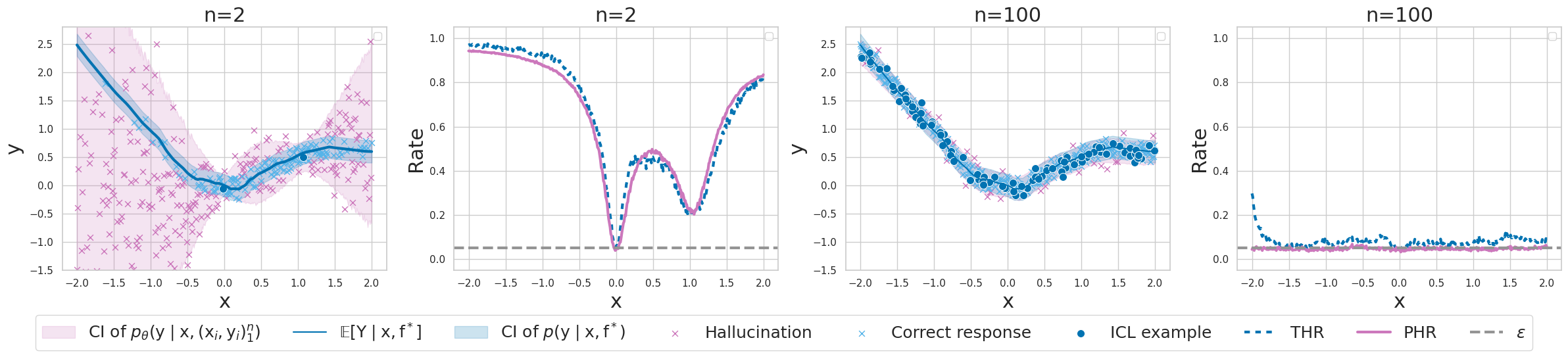
Figure 2: In the first and third panes, we see the neural process’s generated outcomes for $n=2$ and $n=100$. The blue region is the true (1-$\epsilon$)–likely set, while the purple is the likely set when conditioned on the blue data points. The second and fourth panes are the corresponding measures of the PHR and THR across the domain.

Setup. We implement a model with a setup similar to a conditional neural process [46] by modifying the Llama 2 architecture [42] to model sequences of continuous variables. We sample a large set of query-response pairs ($\mathrm{x}$, $\mathrm{y}$) per random re-initialization of the neural network. We define the (1-$\epsilon$)–likely set with $\epsilon=0.05$ such that a response $\mathrm{y}$ is a hallucination if it falls outside of the $95\%$ confidence interval of a given sampled distribution conditioned on $\mathrm{x}$. Training and test data are generated over non-overlapping sets of generated sequences. Example training datasets are shown in Figure 11(a). Example datasets generated by the fit model when initialized with a single random query $\mathrm{x}$ are shown in Figure 11(b). Full model and dataset details are given in Sections E.1 and F.1, respectively.

(a) PHR and THR vs. ${n}$

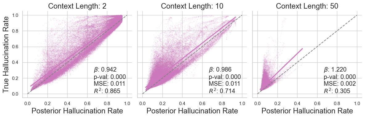
(b) Calibration: THR vs. PHR against different numbers of context examples

Figure 3: Synthetic data: (a) The THR and PHR reduce significantly as the number of contextual examples ${n}$ increases. (b) Calibration evaluation of the posterior hallucination rate against the true probability of hallucination given $\epsilon=0.05$.

Results. The first and third panes of Figure 2 show the model’s generated outcomes for $n=2$ and $n=100$. The blue region represents the true (1-$\epsilon$)–likely set for the response distribution of a specific random ReLU neural network. The purple region represents the model’s (1-$\epsilon$)–likely set when conditioned on the blue data points and a query value $\mathrm{x}$ in the domain [-2, 2]. As more context examples are provided, confidence intervals shrink, and responses $y$ are more likely to fall within the blue region.

The second and fourth panes of Figure 2 show the true probability of hallucination and PHR for $\mathrm{x}$ in the domain [-2, 2] for two settings of $n$. We set $N-n$ to 100 and M to 40. On the left, dips in PHR and hallucination probability at $\mathrm{x}=0$ and $\mathrm{x}=1$ correspond with the ground truth in-context examples. On the right, with larger $n$, both PHR and hallucination probability are low across all $\mathrm{x}$ values. Notably, PHR and hallucination probability align closely throughout the domain. In Section G.1, we show that these findings hold across various settings of the $\epsilon$ parameter value.

In Figure 3(a), we plot the PHR and true probability of hallucination against increasing context lengths, averaged over 200 random test functions. Although PHR aligns well with THR, it underestimates THR, particularly as the number of examples increases. To understand this better, we examine calibration plots between PHR and THR for different numbers of contextual examples in Figure 3(b). For small numbers of contextual examples, PHR closely matches THR, which is encouraging since it is crucial to capture the true probability of hallucination when few examples are present and errors are more likely. These results also support our assumptions about recovering the target estimand through Doob’s Theorem.

To understand the source of the underestimation in the PHR estimator, we consider four potential sources of approximation error. First, the distribution of in-context examples may not be exchangeable due to positional embeddings from the Llama-2 architecture, but this is likely mitigated by training on randomly permuted subsets. Second, Monte-Carlo estimator errors could contribute, but underestimation persists even with increased sample sizes ($M$ or $K$). Third, the finite number of generated examples $(N-n)$ could cause error, but increasing this number beyond 100 shows little bias reduction. Finally, discrepancies between the learned CGM distribution $p_{\bm{\theta}}(\mathrm{y}\mid\mathcal{D}_{n},\mathrm{x})$ and the true distribution $p(\mathrm{y}\mid\mathcal{D}_{n},\mathrm{x})$ can lead to underestimation, as evidenced by differences in confidence intervals around $\mathrm{x}$ values of -2 and 1.5 in Figure 2. This discrepancy likely grows with ${n}$ because accurately modeling $p(\mathrm{y}\mid\mathrm{f}^{\star},\mathrm{x})$ reaches the current limits of in-context learning. Figure 3(a) shows this discrepancy stabilizes with 200 examples, and Figure 3(b) shows PHR becomes a less accurate predictor of the true hallucination rate as the number of examples grows. Improving LLM architecture or training procedures could enhance predictive distribution fidelity and PHR estimates as contextual examples increase.

3.2 Natural language tasks

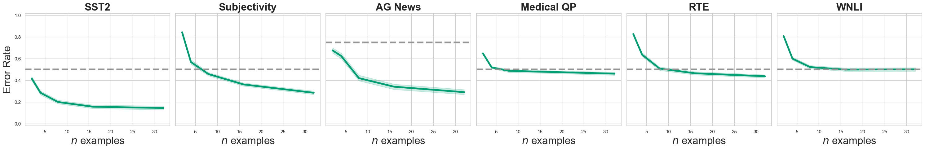
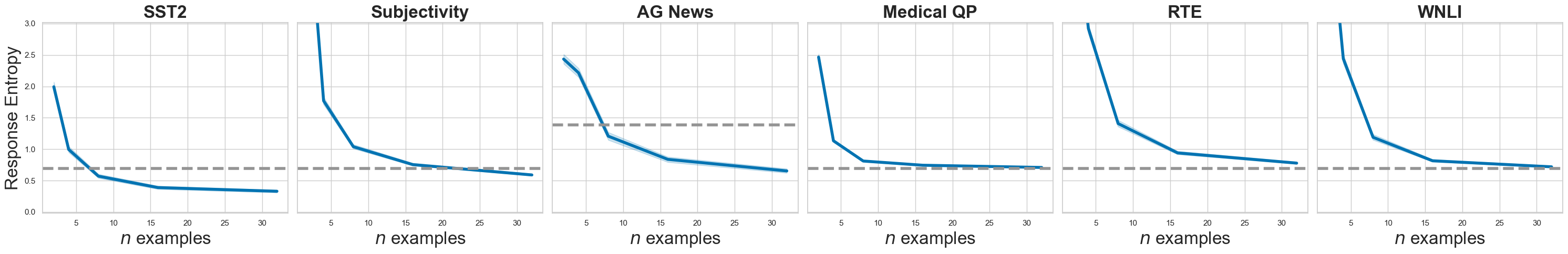
Figure 4: Llama-2-7b: Error Rate (Top green curves) and Response Entropy (Bottom blue curves) on LLM in-context learning tasks. Grey dashed lines represent the error rate and entropy of a random classifier over the set of valid responses.

Here we evaluate the posterior hallucination rate estimator on common natural language in-context learning tasks using the Llama-2 family of LLMs [42]. As we no longer have access to the true $\mathrm{f}^{\star}$ in this setting, we propose a new metric defined below termed Model Hallucination Probability (MPH) that we evaluate the PHR against. We also evaluate against the empirical error rate given ground truth responses.

Setup. We consider tasks defined by six datasets: Stanford Sentiment Treebank (SST2) [47], Subjectivity [48], AG News [6], Medical QP [49], RTE [50], and WNLI [51]. We filter out any queries of length longer than 116 tokens. Full descriptions of these datasets and pre-processing are given in Section F.2.

To implement ICL for a given dataset, we sample a response balanced training set of query/response pairs $\mathcal{D}_{\mathrm{train}}=(\mathrm{x}_{i},\mathrm{y}_{i})_{1}^{n}$. We generate a response $\mathrm{y}$ from the predictive distribution given by a Llama-2 model $p_{\bm{\theta}}(\mathrm{y}\mid\mathcal{D}_{\mathrm{train}},\mathrm{x}_{\mathrm{test}})$. We structure the prompt by adding strings to distinguish between inputs and labels. An example prompt from the Subjectivity dataset is shown in Section E.2.

Figure 4 shows the error rate (top) and response entropy (bottom) of Llama-2-7b. Both metrics decrease and saturate with longer context lengths. For SST2, Subjective, and AG News, the model performs better than random, indicating it can generalize to these tasks ("in-capability"). For Medical QP, RTE, and WNLI, error rates are close to random, indicating poor generalization ("out-of-capability"). The posterior hallucination rate estimator is designed for in-capability tasks and is ill-defined for out-of-capability tasks.

Evaluation metrics. It is a challenge to assess the accuracy of the the posterior hallucination rate on LLM tasks. Although we have a ground truth labeled response for each query, we do not know the ground truth $\mathrm{f}^{\star}$, and therefore we also don’t have access to the $\epsilon$-likely set.

Further, for every query example from the dataset $\mathrm{x}_{\mathrm{test}}$, we only have access to one response $\mathrm{y}$. Because of this, any ambiguity in the true answer for a given query results in the empirical error rate

$$\widehat{E}(\mathrm{x}_{\mathrm{test}},\mathrm{y}_{\mathrm{test}};\bm{\theta})\coloneqq\frac{1}{K}\sum_{i=1}^{K}\mathbbm{1}\{\mathrm{y}_{i}\neq\mathrm{y}_{\mathrm{test}}\},\quad\mathrm{y}_{i}\sim p_{\bm{\theta}}(\mathrm{y}\mid\mathrm{x}_{\mathrm{test}},\mathcal{D}_{\mathrm{train}}),$$ (9)

being a flawed metric for evaluating whether posterior hallucination rate operates as intended. Moreover, even if a dataset contained no ambiguous queries, the posterior hallucination rate will still be vulnerable to estimation error that stems from a discrepancy between the predictive distribution of the LLM and the predictive distribution implied by the task. Therefore, we propose the model hallucination rate (MHR) as a complementary metric

$$\mathrm{MHR}(\mathrm{x}_{\mathrm{test}},\mathcal{D}_{\mathrm{eval}};\bm{\theta})\coloneqq\frac{1}{K}\sum_{i=1}^{K}\mathbbm{1}\Big{\{}\log p_{\bm{\theta}}\big{(}\mathrm{y}_{i}\mid\mathrm{x}_{\mathrm{test}},\mathcal{D}_{\mathrm{train}}\cup\mathcal{D}_{\mathrm{eval}}\big{)}<\widehat{Q}_{\epsilon}^{\mathrm{eval}}\Big{\}},$$

where $\mathrm{y}_{i}\sim p_{\bm{\theta}}(\mathrm{y}\mid\mathrm{x}_{\mathrm{test}},\mathcal{D}_{\mathrm{train}})$, $K$ is the number of response samples and

$$\widehat{Q}_{\epsilon}^{\mathrm{eval}}\coloneqq Q_{\epsilon}\bigg{(}\Big{\{}\log p_{\bm{\theta}}\big{(}\mathrm{y}_{j}\mid\mathrm{x}_{\mathrm{test}},\mathcal{D}_{\mathrm{train}}\cup\mathcal{D}_{\mathrm{eval}}\big{)}\Big{\}}_{j=1}^{K}\bigg{)},\quad\mathrm{y}_{j}\sim p_{\bm{\theta}}(\mathrm{y}\mid\mathrm{x}_{\mathrm{test}},\mathcal{D}_{\mathrm{train}}\cup\mathcal{D}_{\mathrm{eval}}).$$

The MHR assumes that the model posterior $p_{\bm{\theta}}$ is true, and estimates the probability of hallucination when we append the training examples $\mathcal{D}_{\mathrm{train}}$ with ${N}-{n}$ additional ground truth examples $\mathcal{D}_{\mathrm{eval}}$. The posterior hallucination rate marginalizes an equivalent metric over $M$ samples of ${N}-{n}$ generated examples. If the estimator is operating as expected, then it should predict the MHR well. For each task and context length ${n}\in[2,4,8,16,32]$ we sample 50 random training datasets $\mathcal{D}_{\mathrm{train}}$, 50 random evaluation datasets $\mathcal{D}_{\mathrm{eval}}$, and 10 random test samples. We report the mean squared error (MSE), regression coefficient $\beta$, p-value, and coefficient of determination ($R^{2}$) of the posterior hallucination rate as a linear predictor against both the error rate and MHR over all 50x10 test samples at each context length.

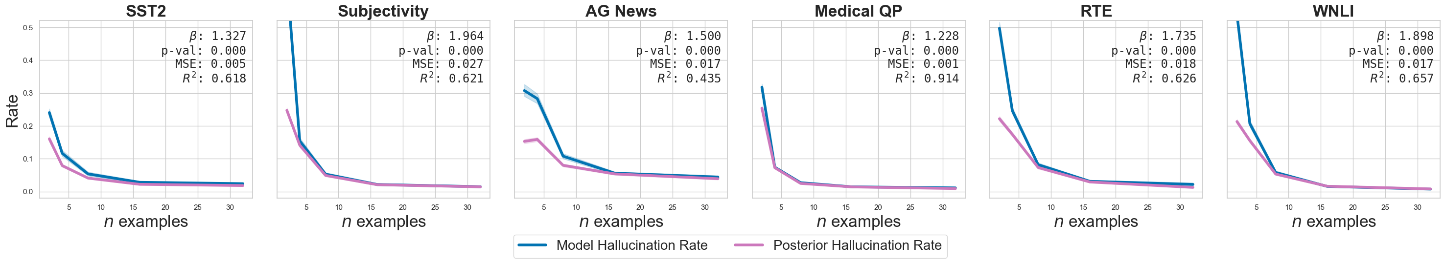
Figure 5: MHR and PHR against number of in-context examples for Llama-2-7b. We set $\epsilon=0.05$, and the Posterior Hallucination Rate accurately tracks the Model Hallucination Probability for all tasks (SST2, Subjective, AG News, Medical QP, RTE, and WNLI). This observation holds across different settings of $\epsilon$, as we show in Figure 17.

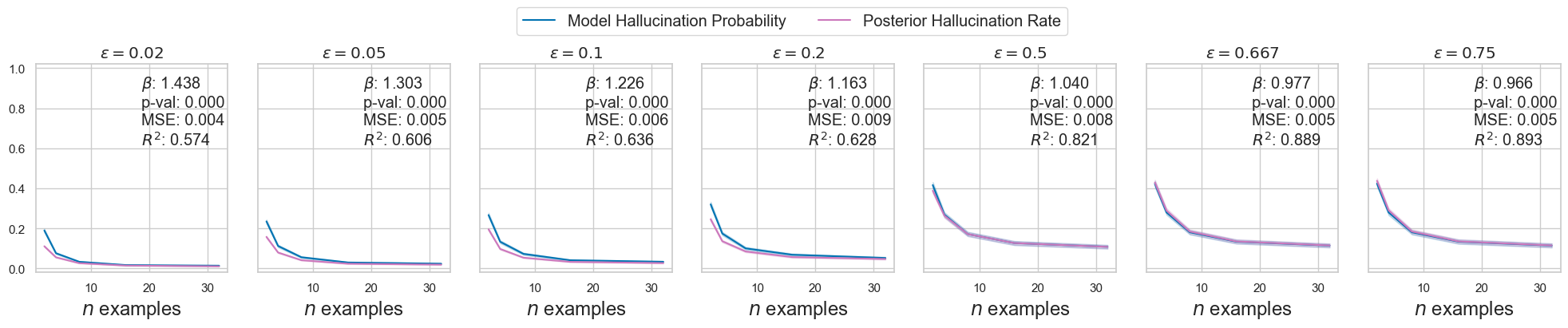
(a) SST2

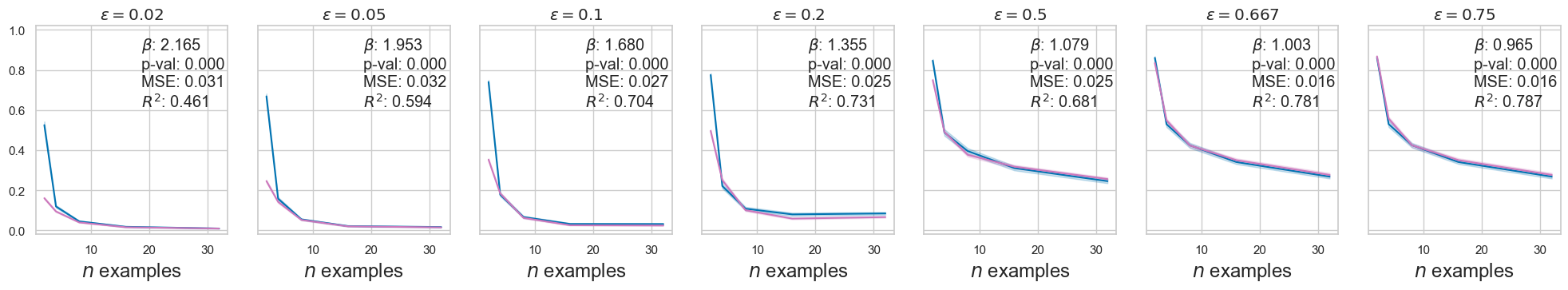
(b) Subjectivity

(c) AG News

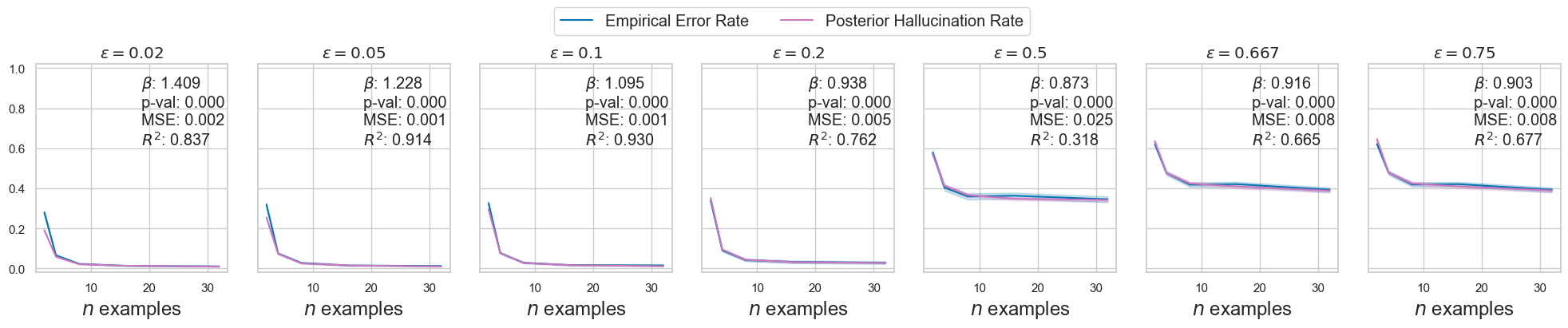
(d) Medical QP

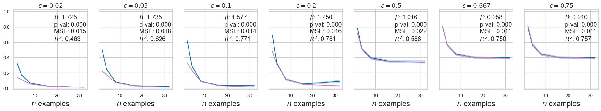
(e) RTE

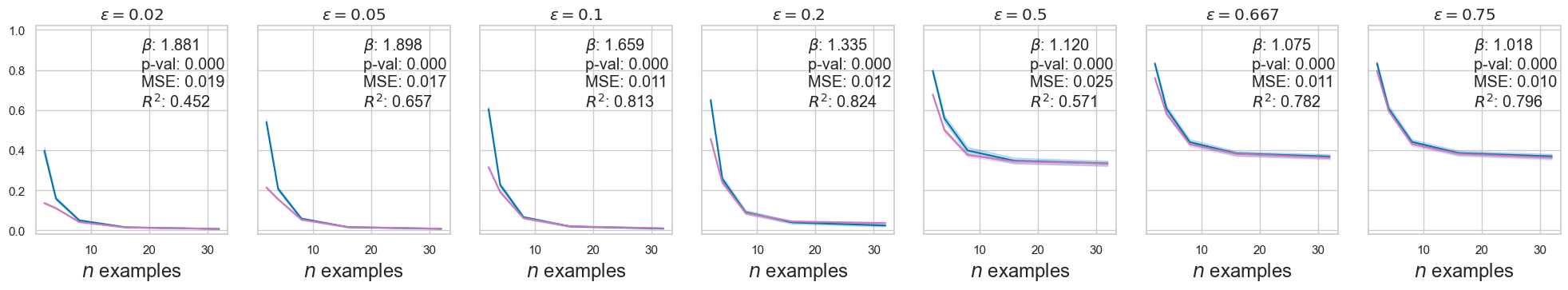
(f) WNLI

Figure 17: Ablating $\epsilon$ for the posterior hallucination rate estimator against the model probability of hallucination for Llama-2-7B.

Results. We report results for Llama-2-7b. We set ${N}-{n}=5$, $M=10$, and $K=50$. Figure 5 plots the MHR and estimated posterior hallucination rate against the number of in-context examples with $\epsilon=0.05$. It shows that the posterior hallucination rate is a good estimator of the MHR. We show that this trend holds for alternative settings of $\epsilon$ in Figure 17 of Appendix G.

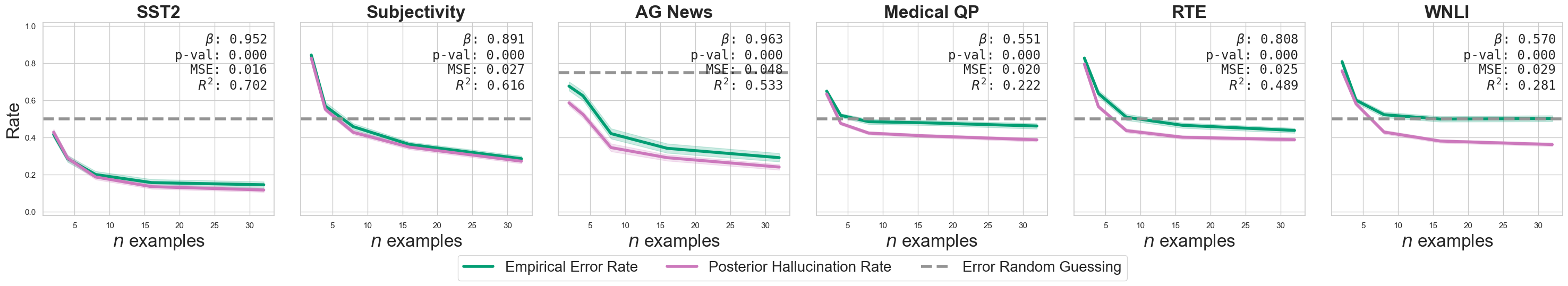
Figure 6: Error rate and PHR against number of in-context examples for Llama-2-7b. When we set $\epsilon$ high (e.g., >0.5), we see that the PHR accurately tracks the Empirical Error Rate for the SST2, Subjective, and AG News datasets. However, for Medical QP the entailment tasks, (RTE and WNLI), the Posterior Hallucination Rate is a considerably worse estimator as these tasks are out-of-capability for Llama-2-7b.

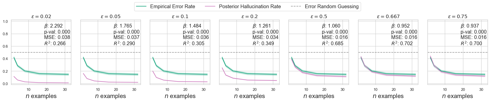
(a) SST2

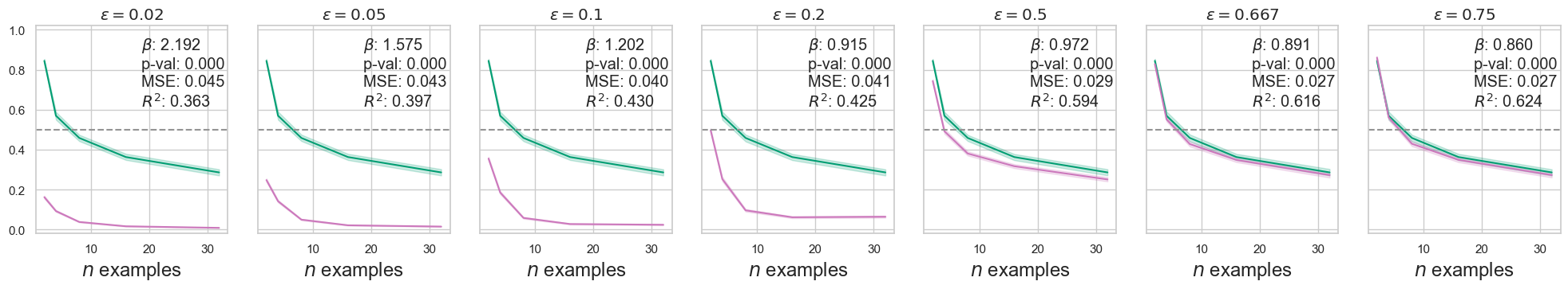
(b) Subjectivity

(c) AG News

(d) Medical QP

(e) RTE

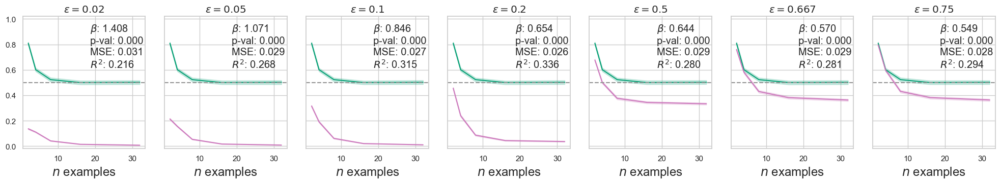
(f) WNLI

Figure 18: Ablating $\epsilon$ for the posterior hallucination rate estimator against the empirical error rate for Llama-2-7B.

Figure 6 plots the empirical error rate and estimated posterior hallucination rate against the number of in-context examples with $\epsilon=0.75$. For the in-capability tasks (SST2, Subjective, and AG News), it shows that the posterior hallucination rate accurately tracks the error rate when $\epsilon$ is set to a high value. For the out-of-capability tasks (Medical QP, RTE, and WNLI), we observe that this is not the case as expected. We ablate the $\epsilon$ parameter and report results in Figure 18 of Appendix G.

4 Discussion

In this work, we have presented a new method for predicting the hallucination rate of in-context learning with conditional generative models. We provide a theoretical justification for our method. In synthetic experiments, we demonstrate that the PHR estimator yields accurate estimates of the true probability of hallucination. With pre-trained LLMs, we demonstrate that it is valuable for predicting the error rate of “in-capability” natural language ICL tasks.

High-fidelity estimation of the PHR relies on two strong assumptions. The first is that the in-context learning problem data admits a de Finetti representation; the second is that the CGM $p_{\bm{\theta}}$ is a faithful estimate of the true distribution $p_{\text{ICL}}$. While our results offer support for the adoption of these assumptions, we also demonstrate that even minor divergences between $p_{\bm{\theta}}$ and $p_{\text{ICL}}$ can result in underestimation. Falck et al. [41] also report instances where properties of the predictive distribution of a pre-trained LLM significantly diverge from those of the true Bayesian posterior predictive distribution for synthetic ICL tasks. These findings highlight a challenge in using PHR as a decision support tool and point to future work on improving the robustness of the PHR estimator or the optimization of conditional generative models for in-context learning.

5 Acknowledgements

The authors would like to thank Amir Feder, Alessandro Grande, Achille Nazaret, Yookoon Park, Kathy Perez, Sebastian Salazar, Claudia Shi, Brian Trippe, Al Tucker, and Luhuan Wu for their reviews, feedback, and support.

Appendix A Related Works

Mechanisms and Capabilities of ICL. Several papers argue that ICL can theoretically and in synthetic scenarios implement learning principles like Bayesian inference or gradient descent [8, 52, 53, 54, 55, 56, 57]. Evidence in actual pre-trained LLMs shows that ICL can be approximated as a kernel regression [58], and parametric approximations to ICL can be derived from the hidden state of the last input demonstration [59, 60]. Practical shortcomings of ICL include dependence on example order [61, 62, 63, 64] and the impact of prediction preferences acquired during pre-training [65, 64, 66, 63, 67]. While future models might improve ICL performance [68], current limitations are clear and are thoroughly investigated in recent work by Falck et al. [41]. These results imply that ICL in real LLMs does not implement perfect Bayesian inference but suggest that LLM predictive uncertainty includes both epistemic and aleatoric components, and LLMs can update uncertainties with new observations.

Uncertainties in LLMs. Our results are supported by evidence that predictive uncertainties of large language models are well-calibrated, even in scenarios requiring epistemic uncertainty [32, 69]. Relatedly, LLM uncertainties have been used to detect hallucinations in free-form generation settings such as question-answering [33, 37, 34, 32, 70, 38, 35, 36, 28, 29, 30]. Although not all these papers explicitly focus on LLM uncertainties, they rely on it implicitly by sampling multiple model completions for a query and quantifying the differences in meaning. Specifically, Kuhn et al. [33] highlight the challenge of isolating uncertainty over semantic meaning from uncertainty over syntax or lexis in free-form generation tasks. While these approaches do not disambiguate aleatoric and epistemic uncertainty, Ahdritz et al. [71], Johnson et al. [72] recently proposed methods to do so in CGMs. However, Ahdritz et al. [71] require access to two LLMs of different parameter counts, and Johnson et al. [72] do not apply their method to LLMs. Additionally, Hu et al. [73] show that Bayesian experimental design can turn LLMs into strategic question askers, and Jeon et al. [74] present a theoretic study on sources of errors in ICL.

Hallucinations in LLMs. In addition to approaches based on uncertainty, a variety of other strategies have been explored to detect or mitigate hallucinations in LLMs: retrieval-augmented generation [9, 10, 11, 12, 13, 14, 15, 16], custom token sampling procedures [17, 18, 19], model fine-tuning to improve uncertainties [20, 21, 22] or reduce hallucinations outright [75], as well as learning to extract or steer truthfulness from hidden states [23, 24, 25, 26, 27].

Neural processes. Neural processes (NPs) [76, 46, 77, 78] are neural network-based non-parametric models trained over a collection of datasets. Similar to ICL, NPs take a collection of datapoints as input and amortize task learning in a single forward pass through the model. For instance, when datasets are drawn from a Gaussian process prior, NPs’ predictive distributions closely approximate the true Bayesian posterior predictive for a given input dataset [7]. NPs have been used successfully for tasks requiring reliable uncertainty estimation, such as Bayesian optimization [76, 78, 40] or active feature acquisition [46]. Recently, Lee et al. [40] applied Doob’s theorem to quantify uncertainties in neural processes.

Martingale Posterior The work closest in spirit to ours is [39] which proposes Martingale Posterior distributions. The idea of that paper is to use the posterior predictive, and not the posterior as the main object for expressing uncertainty. As in this paper, samples from the posterior predictive are used to estimate quantities of interest. Then, by repeated resampling and estimation of the predictive, one obtains a "posterior" over the estimate. Section B.1 contains more details on this work and its relationship to ours. Falck et al. [41] work to formalize this methodology for LLMs. They propose a set of statistical tests to estimate whether an LLM satisfies the “Martingale property.” These tests depend on being able to sample from the true Bayesian model that defines the posterior predictive distribution estimated by the LLM predictive distribution. In their evaluations using synthetic data and pre-trained LLMs, they find that violations of the Martingale property can occur. Moreover, they find that the fidelity of the LLM predictive distribution to the true Bayesian posterior predictive decreases as the length of dataset completions ($N-{n}$) increases. They also derive an epistemic uncertainty estimator based on the posterior covariance over mechanisms, which has connections to the posterior hallucination rate and the mutual information estimand we propose in Appendix D.

Appendix B Further Discussion

B.1 Assumptions

Our proposed algorithm described in Section 2 relies on the existence of an implicit function $\mathrm{F}$ residing in a sufficiently rich space for Doob’s theorem to hold. While this assumption is reasonable for many conditional generative models (CGMs), it may not always be the case. Despite this, we believe our algorithm remains useful and meaningful even in those instances.

An alternative to standard Bayesian methods, as proposed by Fong et al. [39], defines a "posterior" via a constructed sequence of distributions $p(\mathrm{y}_{n}\mid\mathrm{y}_{n-1},\ldots,\mathrm{y}_{1})$. These distributions need not be posterior predictives but simply conditionals that take a sequence of random variables and output a distribution for the next element in the sequence. Their approach involves conditioning on observed data $\mathcal{D}_{n}$ and sampling from the sequence of distributions: $\mathrm{Y}_{n+1}\sim p(\mathrm{y}_{n+1}\mid\mathcal{D}_{n})$, $\mathrm{Y}_{n+2}\sim p(\mathrm{y}_{n+2}\mid\mathrm{Y}_{n+1},\mathcal{D}_{n})$, and so on. These samples are then used to compute a quantity of interest, and by repeating this process multiple times, one obtains a distribution over that quantity. This is precisely the approach we have followed.

The intuitive idea behind this approach is that if each conditional $p(\mathrm{y}_{n+1}\mid\mathrm{y}_{n},\ldots,\mathrm{y}_{0})$ reasonably expresses the uncertainty of a new element in the sequence given the previous $n$ elements, and if any quantity of interest about the distribution could be computed with infinite data, then the method described provides a way to propagate the uncertainty implied by the conditionals to the unobserved data $\mathrm{y}_{n+1},\ldots$, and subsequently to the quantity of interest.

Fong et al. [39] argue that for this approach to be mathematically coherent, a martingale and a convergence condition on the sequence of distributions are necessary. While CGMs may not strictly satisfy these properties, we believe the empirical success of large language models (LLMs) for in-context learning tasks and our empirical results support adopting this methodology due to the usefulness of the conditionals they provide. Therefore, using the posterior predictive as a primary object for defining uncertainty is beneficial, even in cases where no implicit $\mathrm{f}$ exists. Falck et al. [41] summarize such assumptions as the martingale property, and provide an interesting analysis on whether pre-trained LLMs satisfy this property on synthetic ICL tasks.

B.2 Broader Social Impact

Positive social impact. Our work allows for greater intepretability into the responses produced by LLMs and hallucination rate prediction. Being able to discern when a Large Language Model (LLM) is likely to hallucinate is crucial for several reasons, particularly concerning its social impact. In terms of misinformation, if users cannot distinguish between accurate information and hallucinations, they may spread misinformation unknowingly. This can damage the credibility of the platforms using LLMs and the trust users place in AI systems. Further, as LLMs become more commonplace in high-risk sectors like medicine or finance, hallucinated medical advice can be dangerous, leading to harmful health practices or delayed treatment, while erroneous financial information can lead to poor investments or financial loss. Ethically, hallucinations can reinforce or propagate biases and stereotypes if the generated content reflects societal prejudices. This can perpetuate discrimination and inequality. Understanding when hallucinations are likely to occur is vital for holding developers and companies accountable for the content their models produce. Finally, many researchers use LLMs and other CGMs to generate or label data. Hallucinations in this setting can lead to false discoveries and wasted resources.

Being able to accurately predict hallucination rates for given tasks is essential for ensuring that AI systems contribute positively to society. It allows for maintaining trust, safety, ethical standards, and the overall integrity of information dissemination.

Negative social impact. When our model is being used as intended but gives incorrect results (i.e. produces a low estimate of probability of hallucination when the true probability is high), it could inadvertently be reinforcing biases present in hallucinations while increasing user trust in the outputs.

B.3 What kind of uncertainty does the posterior hallucination rate quantify?

Building trustworthy and effective ICL solutions requires understanding why and when incorrect or unexpected responses are generated by a CGM. The ICL literature provides two findings that suggest distinct sources of hallucination.

Figure 7: Llama-2-7b: Error Rate (Top green curves) and Response Entropy (Bottom blue curves) on LLM in-context learning tasks. Grey dashed lines represent the error rate and entropy of a random classifier over the set of valid responses.

The first finding is that error rate and prediction entropy decreases and saturates with an increasing number of examples [64]. This trend is illustrated in Figure 7 using the Llama-2-7b model [42] on a set of natural language ICL tasks. This finding indicates that one source of hallucination is an insufficient number of relevant in-context examples.

The second finding from the literature is that there are still many tasks for which ICL performs poorly. For example, the response accuracy of Gemini Pro 1.5 given several in-context examples from the American Mathematics Competition is only 37.2%, implying that the model would hallucinate an incorrect response at a rate of 62.8% [3]. We hypothesize that regardless of the number of relevant in-context examples, the model may lack the capacity to answer a specific user query from a complex or new domain accurately. This hypothesis is illustrated using Llama-2-7B by comparing the graphs of the first three tasks (SST2 [47], Subjective [48], and AG News [6]) to the graph of the WNLI task [51]) in Figure 4. While the error rate and response entropy for each of the first three tasks improves significantly over random guessing with more examples, both measures appear to saturate near the random baseline for the WNLI task. The second source of hallucinations is then associated with whether a model has the capacity to factually answer queries for an ICL task.

This work focuses on the first source of hallucinations. That is, the posterior hallucination rate is concerned with estimating the rate of hallucinations that stem from a lack of relevant context, and not those that stem from a lack of model capacity. The predictive distribution encodes response variety coming from several sources, and this variety is closely tied to the ways in which a model can generate a hallucination. We discuss these sources of response variety—or uncertainty—below and their relation to hallucinations and the posterior hallucination rate.

Aleatoric Uncertainty. The $(1-\epsilon)$–likely set defined by a given mechanism $\mathrm{f}^{*}$ reflects an irreducible component of response uncertainty. To illustrate the concept of irreducible (sometimes called “aleatoric”) response uncertainty, imagine an LLM fit to vast corpora containing many calculus examples such that it has the capacity for integration. Consider,

Prompt 1:

    fill in the blanks: the integral of x^2 with respect to x on     the interval [-3, 3] is ␣.

If an LLM effectively models the mechanism associated with integration datasets, then response variety will be determined by all the different ways the model can generate the correct response: e.g., 18, eighteen, $\frac{3^{3}}{3}-\frac{\text{-}3^{3}}{3}$, $9+9$, $2*9$, XVIII, etc. Uncertainty reflecting the plurality of ways to communicate the same meaning is commonly referred to as syntactic uncertainty [33], which is considered irreducible in this particular example. However, in language tasks, irreducible uncertainty need not be syntactic by necessity.

To enrich this concept, consider the same LLM and

Prompt 2:

    fill in the blanks: the integral of ␣, with respect to x on     the interval [-3, 3] is ␣.

In addition to the syntactically different ways to specify a particular function ($x^{2}$, $x$ squared, $xx$, …) and the corresponding result (18, eighteen, XVIII, …), response variety also depends on the semantically different integrands that could fill the first blank ($x^{3}$, $\cos{(x)}$, $\exp{(x)}$, $2xy$, $\dots$) and the semantically different possible results. This additional variety is emblematic of semantic uncertainty [33]. However, while high semantic uncertainty can be indicative of hallucinations, it is not a problem in this example because the imputation of any sensible function and answer could still be valid under the mechanism associated with integration datasets. That is, given Prompt 2, uncertainty over semantically different functions is expected and even desirable.

This pair of examples illustrate an important insight; irreducible uncertainty is mechanism relative. If, for example, we are in a simple question answering setting and the mechanism defines a $(1-\epsilon)$–likely set over correct responses, then, equivocating irreducible and syntactic uncertainty may be appropriate. However, in the second example we show that this decomposition is not necessarily appropriate.

Type I epistemic uncertainty. We return to Prompt 1 and give two examples that illustrate an uncertainty about mechanisms $\mathrm{f}$ that is reducible. First, consider a setting where the user desires the response in terms of a reduced fraction. There are two obvious ways that the user could augment Prompt 1 to reduce the uncertainty over mechanisms yielding integer, word, fraction, etc. responses. (1) the user could simply replace “fill in the blanks” with “fill in the blank with a reduced fraction.” (2) the user could take an ICL approach and augment the prompt with a number of examples:

Prompt 3:

    Input: the integral of x^3 with respect to x on the interval [-1, 6]     Label: $\frac{1295}{4}$     Input: the integral of x^6 with respect to x on the interval [-2, 2]     Label: 0 / 7.     Input: the integral of x^2 with respect to x on the interval [-3, 3]     Label:

The first choice may result in reducing all uncertainty about which mechanism to sample responses from. For the second choice, we can imagine a progressive reduction in uncertainty about the appropriate mechanism as more examples are added in-context. For example, if we were to see the two provided examples, we may still be uncertain about whether to respond with a number or a fraction, or whether to respond with any correct fraction or the reduced fraction. For example, given the context, a response of $\frac{54}{3}$ would be as plausible as the desired $\frac{18}{1}$. It may not be until the prompt included an example like, “the integral of $x^{3}$ with respect to $x$ on the interval $[2,4]$ is $60/1$,” until all uncertainty about the mechanism is resolved. We propose that this explains why we see a reduction in the error rate and response entropy in a task like WNLI that is “out-of-capacity” for Llama-2-7B. That is, as we provide more in-context examples, the predictive distribution can be more aligned with the set of acceptable responses, even though those responses may still be incorrect.

The preceding example illustrated a hallucination as a misaligned response, now let’s turn to an example of a non-factual response. Returning to Prompt 1, imagine now that the model generates the response 42. Why did it do this? A plausible answer could be that the model cannot do integration. We will touch on this possibility next, but first let’s consider an equally interesting case. We know from the few-shot and chain-of-thought prompting literature [79, 14, 30], that augmenting the context can have significant effects on ICL accuracy. For example, consider the hypothetical setting where the LLM has “grokked” algebra, but only has the superficial capacity to output a number when completing definite integrals. Or maybe the model has capacity to do integration, but the format of the examples and query is not common in the training corpora. The LLM then may actually have the capacity to answer the question given some clever prompting. For example,

Prompt 4:

    Input: the integral of x^3 with respect to x on the interval [-1, 6]     Label: 6^4 / 4  - -1^4 / 4 = 1295 / 4     Input: the integral of x^3 with respect to x on the interval [2, 4]     Label: 4^4 / 4 - 2^4 / 4 = 60 / 1.

    ...     Input: the integral of x^6 with respect to x on the interval [-2, 2]     Label: 2^7 / 7 - -2^7 / 7 = 0 / 7     Input: the integral of x^2 with respect to x on the interval [-3, 3]     Label:

Again, as the prompt contains more examples that translate the form of the query into a suitable format, we can expect that the uncertainty about the answer will reduce. For conditional models in general, we will call this Type I epistemic uncertainty, which could also be understood as in-context epistemic uncertainty. Both of these examples illustrate hallucinations that are due to insufficient context.

Type II epistemic uncertainty. Let’s return to Prompt 1, but this time imagine an LLM fit to a corpus not containing any examples from calculus or related mathematical fields. Or perhaps we could imagine an LLM with finite capacity that for whatever reason does not have the capacity to answer integrals. What do we do when the model generates “Dua Lipa?” What do we do when the model outputs members of the set $\{17,137,\text{Dua Lipa},\text{Wednesday},\dots\}$? We say that the response should have high Type II epistemic uncertainty because the LLM has not acquired the capacity to model the mechanism class, $\mathrm{F}$, corresponding to integrals. This could also be understood as in-weights $\bm{\theta}$ epistemic uncertainty. In the example of Prompt 4, imagine if there were no number of exemplars that could induce a correct response.

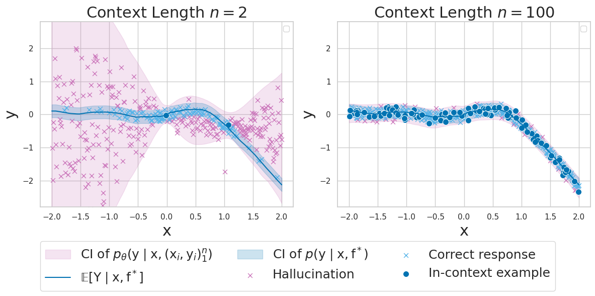
(a) Type I

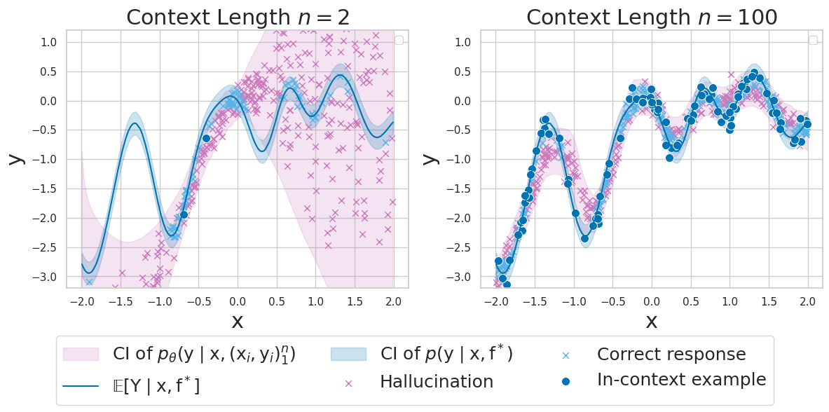
(b) Type II

Figure 8: Comparing different sources of hallucination for regression models. Figure 8(a) illustrates hallucinations due to Type I epistemic uncertainty. As the context length increases, the predictive distribution concentrates around the true distribution and the model hallucinates less. Figure 8(b) illustrates hallucinations due to Type II epistemic uncertainty. Given data from an out-of-distribution function, the predictive distribution may not cover the true distribution. Moreover, the model still hallucinates significantly even when Type I epistemic uncertainty is minimized as the number of in-context examples is large.

When a condition generative model $p_{\bm{\theta}}$ is a good estimator of the true distribution $p$, the posterior hallucination rate—and mutual information quantity we propose in Appendix D—are designed to estimate Type I epistemic uncertainty. We leave the important work of estimating the posterior hallucination rate when the CGM is not a good estimator (under Type II epistemic uncertainty) to future work.

Appendix C Proof of Theorems in Main Text

We begin by stating a lemma that will be useful throughout.

Lemma C.1.

Assume that the conditions of Theorem 1 hold for $\mathrm{F}$ and $(\mathrm{X},\mathrm{Y})$, then for a fixed dataset and query $\mathcal{D}_{n},\mathrm{x}$ and under a probability model where $\mathrm{F}\sim p(\mathrm{f}\mid\mathcal{D}_{n})$ and $(\mathrm{X}_{i},\mathrm{Y}_{i})\sim p(\mathrm{x},\mathrm{y}\mid\mathrm{F})$, then

$$\log p(\mathrm{Y}\mid\mathrm{x},\mathrm{F})=\lim_{n\to\infty}\log p\left(\mathrm{Y}\mid\mathrm{x},(\mathrm{X},\mathrm{Y})_{1}^{n}\right)$$

almost surely.

Proof.

For a fixed $\mathrm{y},\mathrm{x}$, let $g(\mathrm{f})=p(\mathrm{y}\mid\mathrm{x},\mathrm{F})$ and then apply Doob’s theorem on the probability model. Then it is the case that

$$g(\mathrm{F}) =\lim_{n\to\infty}\operatorname*{\mathbb{E}}_{\mathrm{F}\sim p(\mathrm{f}\mid\mathcal{D}_{n})}[p(\mathrm{y}\mid\mathrm{F},\mathrm{x})\mid(\mathrm{X}_{i},\mathrm{Y}_{i})^{n}]$$ (10)

$$=\lim_{n\to\infty}\int p(\mathrm{y}\mid\mathrm{F},\mathrm{x})d\mathrm{P}(\mathrm{F}\mid(\mathrm{X}_{i},\mathrm{Y}_{i})^{n})$$ (11)

$$=\lim_{n\to\infty}\int p(\mathrm{y}\mid\mathrm{F},\mathrm{x})d\mathrm{P}(\mathrm{F}\mid(\mathrm{X}_{i},\mathrm{Y}_{i})^{n},\mathrm{x})$$ (12)

$$=\lim_{n\to\infty}p(\mathrm{y}\mid\mathrm{x},(\mathrm{X}_{i},\mathrm{Y}_{i})^{n})$$ (13)

where Equation 12 holds because $\mathrm{x}$ is independent of $\mathrm{F}$. Taking logs at both sides and using the continuity of the logarithm, we obtain

$$\log g(\mathrm{F})=\lim_{n\to\infty}\log p(\mathrm{y}|\mathrm{x},(\mathrm{X}_{i},\mathrm{Y}_{i})_{1}^{n})$$

and because this holds for all $\mathrm{y}$, it must hold for the random variable $\mathrm{Y}$. ∎

Now we restate the main theorem with proof:
See 2

Proof.

Define an alternative probability model such that $\mathrm{F}\sim p(\mathrm{f}\mid\mathcal{D}_{n})$ and $(\mathrm{X}_{i},\mathrm{Y}_{i})\sim p(\mathrm{x},\mathrm{y}\mid\mathrm{F})$. Let $p_{a}$, $\operatorname*{\mathbb{E}}_{a}$, $Q_{a,\epsilon}$ and $\mathrm{P}_{a}$ denote the relevant quantities computed with respect to this alternative probability model.

First, note that by expanding the definition of $Q_{a,\epsilon}(\mathrm{f},\mathrm{x})$ under this new probability model

$$Q_{a,\epsilon}(\mathrm{F},\mathrm{x}) =\inf\left\{q\in\mathbb{R}:\epsilon\leq\mathrm{P}_{a}(\log p_{a}(\mathrm{Y}\mid\mathrm{x},\mathrm{F})\leq q\mid\mathrm{F},\mathrm{x})\right\}$$ (14)

$$Q_{a,\epsilon}(\mathrm{F},\mathrm{x}) =\inf\left\{q\in\mathbb{R}:\epsilon\leq\mathrm{P}_{a}(\log p_{a}(\mathrm{Y}\mid\mathrm{x},\mathrm{F})\leq q\mid\mathrm{F},\mathrm{x},(\mathrm{X},\mathrm{Y})_{1}^{\infty})\right\}$$ (15)

$$=\inf\left\{q\in\mathbb{R}:\epsilon\leq\mathrm{P}_{a}\left(\lim_{N\to\infty}\log p_{a}(\mathrm{Y}\mid\mathrm{x},(\mathrm{X}_{i},\mathrm{Y}_{i})_{1}^{N})\leq q\mid\mathrm{F},\mathrm{x},(\mathrm{X},\mathrm{Y})_{1}^{\infty}\right)\right\}$$ (16)

where we used the fact that $\mathrm{Y}\perp(\mathrm{X},\mathrm{Y})_{1}^{\infty}\mid\mathrm{F},\mathrm{x}$ in Equation 15. For simplicity, we will use $p(\cdot|(\mathrm{X}_{i},\mathrm{Y}_{i})_{1}^{\infty})$ to denote $\lim_{N\to\infty}p(\cdot\mid\left(\mathrm{X}_{i},\mathrm{Y}_{i})_{1}^{N}\right)$ with similar conventions from other quantities. Now, applying Doob’s to $g(\mathrm{f})=\mathrm{P}_{a}(\log p_{a}(\mathrm{Y}\mid\mathrm{x},(\mathrm{X}_{i},\mathrm{Y}_{i})_{1}^{\infty})\leq q\mid\mathrm{f},\mathrm{x},(\mathrm{X}_{i},\mathrm{Y}_{i})_{1}^{\infty})$ we get that almost surely

$$\mathrm{P}_{a}( \log p_{a}(\mathrm{Y}\mid\mathrm{x},(\mathrm{X}_{i},\mathrm{Y}_{i})_{1}^{\infty})\leq q\mid\mathrm{F},\mathrm{x},(\mathrm{X}_{i},\mathrm{Y}_{i})_{1}^{\infty})$$ (17)

$$=\lim_{N\to\infty}\operatorname*{\mathbb{E}}_{\mathrm{F}\sim p(\mathrm{f}\mid\mathcal{D}_{n})}\left[\mathrm{P}_{a}(\log p_{a}(\mathrm{Y}\mid\mathrm{x},(\mathrm{X}_{i},\mathrm{Y}_{i})_{1}^{\infty})\leq q\mid\mathrm{F},\mathrm{x},(\mathrm{X}_{i},\mathrm{Y}_{i})_{1}^{\infty})\mid(\mathrm{X}_{i},\mathrm{Y}_{i})_{1}^{N}\right]$$ (18)

$$=\lim_{N\to\infty}\mathrm{P}_{a}(\log p_{a}(\mathrm{Y}\mid\mathrm{x},(\mathrm{X}_{i},\mathrm{Y}_{i})_{1}^{\infty})\leq q\mid(\mathrm{X}_{i},\mathrm{Y}_{i})_{1}^{N})$$ (19)

$$=\mathrm{P}_{a}(\log p_{a}(\mathrm{Y}|\mathrm{x},(\mathrm{X}_{i},\mathrm{Y}_{i})_{1}^{\infty})\leq q\mid(\mathrm{X}_{i},\mathrm{Y}_{i})_{1}^{\infty})$$ (20)

where we used Doob’s on Equation 18 and the tower property in Equation 19. Plugging this back in Equation 16 we obtain

$$Q_{a,\epsilon}(\mathrm{F},\mathrm{x}) =\inf\left\{q\in\mathbb{R}:\epsilon\leq\mathrm{P}_{a}(\log p_{a}(\mathrm{Y}\mid\mathrm{x},(\mathrm{X}_{i},\mathrm{Y}_{i})_{1}^{\infty})\leq q\mid(\mathrm{X}_{i},\mathrm{Y}_{i})_{1}^{\infty})\right\}$$ (21)

$$=Q_{a,\epsilon}((\mathrm{X}_{i},\mathrm{Y}_{i})_{1}^{\infty},\mathrm{x})$$ (22)

To complete the proof, note that

$$\iint\mathbbm{1}\big{\{}\log p(\mathrm{y}\mid\mathrm{x},\mathrm{f})<Q_{\epsilon}(\mathrm{f},\mathrm{x})\big{\}}d\mathrm{P}(\mathrm{f}\mid\mathcal{D}_{n})d\mathrm{P}(y\mid\mathrm{x},\mathcal{D}_{n})$$ (23)

$$=\iint\mathbbm{1}\big{\{}\log p_{a}(\mathrm{y}\mid\mathrm{x},\mathrm{f})<Q_{a,\epsilon}(\mathrm{f},\mathrm{x})\big{\}}d\mathrm{P}_{a}(\mathrm{f})d\mathrm{P}(y\mid\mathrm{x},\mathcal{D}_{n})$$ (24)

where we changed the probability spaces from $p$ to $p_{a}$. This is justified because $p_{a}(\mathrm{y}\mid\mathrm{x},\mathrm{f})=p(\mathrm{y}\mid\mathrm{x},\mathrm{f},\mathcal{D}_{n})=p(\mathrm{y}\mid\mathrm{x},\mathrm{f})$ where we used the independence of $\mathrm{Y}$ on $\mathcal{D}_{n}$ once $\mathrm{f}$ is known, the fact that $p_{a}(\mathrm{f})=p(\mathrm{f}\mid\mathcal{D}_{n})$ by definition, and the fact that for the quantile function $Q_{a,\epsilon}(\mathrm{f},\mathrm{x})=Q_{\epsilon}(\mathrm{f},\mathrm{x})$ because

$$\mathrm{P}_{a}\left(\log p_{a}(\mathrm{Y}\mid\mathrm{x},\mathrm{F})\leq q\mid\mathrm{F},\mathrm{x}\right)=\mathrm{P}\left(\log p(\mathrm{Y}\mid\mathrm{x},\mathrm{F})\leq q\mid\mathrm{F},\mathrm{x}\right)$$ (25)

due again to the independence of $\mathrm{Y}$ on the dataset $\mathcal{D}_{n}$ once $\mathrm{f}$ is known. Finally we have (abusing notation using $(\mathrm{x},\mathrm{y})_{n+1}^{\infty}$ to refer to $(\mathrm{x},\mathrm{y})_{n+1}^{\infty}$ in the original probability space but also $(\mathrm{x}_{i},\mathrm{y}_{i})_{1}^{\infty}$ in the alternative probability space as they have the same distribution):

$$h_{\epsilon}(\mathrm{x})= \iint\mathbbm{1}\big{\{}\log p_{a}(\mathrm{y}\mid\mathrm{x},\mathrm{f})<Q_{a,\epsilon}(\mathrm{f},\mathrm{x})\big{\}}d\mathrm{P}_{a}(\mathrm{f})d\mathrm{P}(\mathrm{y}\mid\mathrm{x},\mathcal{D}_{n})$$ (26)

$$= \iint\mathbbm{1}\big{\{}\log p_{a}(\mathrm{y}\mid\mathrm{x},\mathrm{f})<Q_{a,\epsilon}(\mathrm{f},\mathrm{x})\big{\}}d\mathrm{P}_{a}(\mathrm{f},(\mathrm{x},\mathrm{y})_{n+1}^{\infty})d\mathrm{P}(\mathrm{y}\mid\mathrm{x},\mathcal{D}_{n})$$ (27)

$$= \iint\mathbbm{1}\big{\{}\log p_{a}(\mathrm{y}\mid\mathrm{x},(\mathrm{x},\mathrm{y})_{n+1}^{\infty})<Q_{a,\epsilon}((\mathrm{x},\mathrm{y})_{n+1}^{\infty},\mathrm{x})\big{\}}d\mathrm{P}_{a}(\mathrm{y}\mid\mathrm{x})d\mathrm{P}_{a}(\mathrm{f},(\mathrm{x},\mathrm{y})_{n+1}^{\infty})$$ (28)

$$= \iint\mathbbm{1}\big{\{}\log p_{a}(\mathrm{y}\mid\mathrm{x},(\mathrm{x},\mathrm{y})_{n+1}^{\infty})<Q_{a,\epsilon}((\mathrm{x},\mathrm{y})_{n+1}^{\infty},\mathrm{x})\big{\}}d\mathrm{P}(\mathrm{y}\mid\mathcal{D}_{n},\mathrm{x})d\mathrm{P}(\mathrm{f},(\mathrm{x},\mathrm{y})_{n+1}^{\infty}\mid\mathcal{D}_{n})$$ (29)

$$= \iint\mathbbm{1}\big{\{}\log p_{a}(\mathrm{y}\mid\mathrm{x},(\mathrm{x},\mathrm{y})_{n+1}^{\infty})<Q_{a,\epsilon}((\mathrm{x},\mathrm{y})_{n+1}^{\infty},\mathrm{x})\big{\}}d\mathrm{P}(\mathrm{y}\mid\mathcal{D}_{n},\mathrm{x})d\mathrm{P}((\mathrm{x},\mathrm{y})_{n+1}^{\infty}\mid\mathcal{D}_{n})$$ (30)

Where Equation 27 is justified by because $(\mathrm{x},\mathrm{y})_{n+1}^{\infty}$ doesn’t appear in the term inside, Equation 28 is justified by the arguments above and Lemma C.1, and Equation 30 is a result of marginalizing $\mathrm{f}$ out. The last thing to point out is that $p_{a}(\mathrm{y}\mid\mathrm{x},(\mathrm{x},\mathrm{y})_{n+1}^{\infty})=p(\mathrm{y}\mid\mathrm{x},(\mathrm{x}_{i},\mathrm{y}_{i})_{1}^{\infty})$ and $Q_{a,\epsilon}((\mathrm{x},\mathrm{y})_{n+1}^{\infty},\mathrm{x})=Q_{\epsilon}((\mathrm{x}_{i},\mathrm{y}_{i})_{1}^{\infty},\mathrm{x})$ because

$$\mathrm{P}_{a} \left(\log p_{a}(\mathrm{Y}\mid\mathrm{x},(\mathrm{x},\mathrm{y})_{n+1}^{\infty})\leq q\mid\mathrm{x},(\mathrm{x},y)_{n+1}^{\infty}\right)$$

$$=\mathrm{P}\left(\log p(\mathrm{Y}\mid\mathrm{x},(\mathrm{x}_{i},\mathrm{y}_{i})_{1}^{\infty})\leq q\mid\mathrm{x},(\mathrm{x}_{i},\mathrm{y}_{i})_{1}^{\infty}\right)$$

Using this fact in Equation 30 yields the theorem.

∎

Appendix D Mutual Information

In the main paper we focus on developing the posterior hallucination rate; however, there are other quantities that can also be used to predict model performance. A common quantity used for this purpose in Bayesian machine learning is the posterior mutual information between $\mathrm{F}$ and $\mathrm{Y}$, ${\color[rgb]{0.06640625,0.46484375,0.19921875}\mathrm{I}(\mathrm{Y};\mathrm{F}\mid\mathrm{x},\mathcal{D}_{n})}$, sometimes referred to as the epistemic uncertainty. The reason for this name is that when we define the total predictive uncertainty to be ${\color[rgb]{0.53515625,0.1328125,0.33203125}\mathrm{H}(\mathrm{Y}\mid\mathrm{x},\mathcal{D}_{n})}$ and the aleatoric uncertainty—the component of the uncertainty that can’t be reduced—as ${\color[rgb]{0.19921875,0.1328125,0.53515625}\operatorname*{\mathbb{E}}_{p(\mathrm{f}\mid\mathrm{x},\mathcal{D}_{n})}[\mathrm{H}(\mathrm{Y}\mid\mathrm{f},\mathrm{x})]}$, then the difference is the reducible component, and by the definition of mutual information

$${\color[rgb]{0.06640625,0.46484375,0.19921875}\underbrace{{\color[rgb]{0.06640625,0.46484375,0.19921875}\mathrm{I}(\mathrm{Y};\mathrm{F}\mid\mathrm{x},\mathcal{D}_{n})}}_{\text{Epistemic uncertainty}}}={\color[rgb]{0.53515625,0.1328125,0.33203125}\underbrace{{\color[rgb]{0.53515625,0.1328125,0.33203125}\mathrm{H}(\mathrm{Y}\mid\mathrm{x},\mathcal{D}_{n})}}_{\text{Predictive uncertainty}}}-{\color[rgb]{0.19921875,0.1328125,0.53515625}\underbrace{{\color[rgb]{0.19921875,0.1328125,0.53515625}\operatorname*{\mathbb{E}}_{p(\mathrm{f}\mid\mathrm{x},\mathcal{D}_{n})}[\mathrm{H}(\mathrm{Y}\mid\mathrm{f},\mathrm{x})]}}_{\text{Aleatoric uncertainty}}}$$

D.1 Estimators

Inspired by the methodology in the paper, we follow a similar process for obtaining approximate estimates of the aleatoric uncertainty and epistemic uncertainties.

In particular we let,

$${\color[rgb]{0.19921875,0.1328125,0.53515625}\mathrm{H}_{\bm{\theta}}(\mathrm{Y}\mid\mathrm{F},(\mathrm{x}_{i},\mathrm{y}_{i})_{1}^{n},\mathrm{x})}\coloneqq{\color[rgb]{0.19921875,0.1328125,0.53515625}-\int g^{\mathrm{H}}_{\bm{\theta}}((\mathrm{x}_{i},\mathrm{y}_{i})_{1}^{N},\mathrm{x})d\mathrm{P}_{\bm{\theta}}(\mathrm{x}^{{n}+1:{N}}\mid(\mathrm{x}_{i},\mathrm{y}_{i})_{1}^{n})},$$

where

$${\color[rgb]{0.19921875,0.1328125,0.53515625}g^{\mathrm{H}}_{\bm{\theta}}((\mathrm{x}_{i},\mathrm{y}_{i})_{1}^{N},\mathrm{x})}\coloneqq{\color[rgb]{0.19921875,0.1328125,0.53515625}\int\log p_{\bm{\theta}}(\mathrm{y}\mid(\mathrm{x}_{i},\mathrm{y}_{i})_{1}^{N},\mathrm{x}))d\mathrm{P}_{\bm{\theta}}(\mathrm{y}\mid(\mathrm{x}_{i},\mathrm{y}_{i})_{1}^{N},\mathrm{x})},$$ (31)

and ${N}-{n}$ is a practical number of generated examples. This model approximation for the aleatoric entropy allows us to define a model approximation for the mutual information.

$${\color[rgb]{0.06640625,0.46484375,0.19921875}\mathrm{I}_{\bm{\theta}}(\mathrm{Y};\mathrm{F}\mid(\mathrm{x}_{i},\mathrm{y}_{i})_{1}^{n},\mathrm{x})}\coloneqq{\color[rgb]{0.53515625,0.1328125,0.33203125}\mathrm{H}_{\bm{\theta}}(\mathrm{Y}\mid(\mathrm{x}_{i},\mathrm{y}_{i})_{1}^{n},\mathrm{x})}-{\color[rgb]{0.19921875,0.1328125,0.53515625}\mathrm{H}_{\bm{\theta}}(\mathrm{Y}\mid\mathrm{F},(\mathrm{x}_{i},\mathrm{y}_{i})_{1}^{n},\mathrm{x})}.$$ (32)

In turn, we can construct practical Monte-Carlo estimators for $\color[rgb]{0.53515625,0.1328125,0.33203125}{\mathrm{H}_{\bm{\theta}}(\mathrm{Y}\mid(\mathrm{x}_{i},\mathrm{y}_{i})_{1}^{n},\mathrm{x})}$, $\color[rgb]{0.19921875,0.1328125,0.53515625}{g^{\mathrm{H}}_{\bm{\theta}}((\mathrm{x}_{i},\mathrm{y}_{i})_{1}^{N},\mathrm{x})}$, and $\color[rgb]{0.19921875,0.1328125,0.53515625}{\mathrm{H}_{\bm{\theta}}(\mathrm{Y}\mid\mathrm{F},(\mathrm{x}_{i},\mathrm{y}_{i})_{1}^{n},\mathrm{x})}$ using predictive resampling [39]. These estimators are described below and the predictive resampling algorithm is described in Algorithm 3.

Predictive entropy.

$$\widehat{H}_{\bm{\theta}}(\mathrm{Y}\mid(\mathrm{x}_{i},\mathrm{y}_{i})_{1}^{n},\mathrm{x})\coloneqq-\frac{1}{\mathrm{M}}\sum_{i=1}^{\mathrm{M}}\log p_{\bm{\theta}}(\mathrm{y}_{i}\mid(\mathrm{x}_{i},\mathrm{y}_{i})_{1}^{n},\mathrm{x}),\quad\mathrm{y}_{i}\sim p_{\bm{\theta}}(\mathrm{y}\mid(\mathrm{x}_{i},\mathrm{y}_{i})_{1}^{n},\mathrm{x})$$ (33)

Aleatoric entropy.

$$\widehat{g}^{\mathrm{H}}_{\bm{\theta}}((\mathrm{x}_{i},\mathrm{y}_{i})_{1}^{N},\mathrm{x})\coloneqq-\frac{1}{\mathrm{M}}\sum_{i=1}^{\mathrm{M}}\log p_{\bm{\theta}}(\mathrm{y}_{i}\mid(\mathrm{x}_{i},\mathrm{y}_{i})_{1}^{N},\mathrm{x}),\quad\mathrm{y}_{i}\sim p_{\bm{\theta}}(\mathrm{y}\mid(\mathrm{x}_{i},\mathrm{y}_{i})_{1}^{N},\mathrm{x})$$ (34)

$$\widehat{H}_{\bm{\theta}}(\mathrm{Y}\mid\mathrm{F},(\mathrm{x}_{i},\mathrm{y}_{i})_{1}^{n},\mathrm{x})\coloneqq\mathrm{PredictiveResampling}\big{(}\mathrm{x},(\mathrm{x}_{i},\mathrm{y}_{i})_{1}^{n},\widehat{g}^{\mathrm{H}}_{\bm{\theta}}((\mathrm{x}_{i},\mathrm{y}_{i})_{1}^{N},\mathrm{x})\big{)}$$ (35)

Mutual information

$$\widehat{\mathrm{I}}_{\bm{\theta}}(\mathrm{Y};\mathrm{F}\mid(\mathrm{x}_{i},\mathrm{y}_{i})_{1}^{n},\mathrm{x})\coloneqq\widehat{\mathrm{H}}_{\bm{\theta}}(\mathrm{Y}\mid(\mathrm{x}_{i},\mathrm{y}_{i})_{1}^{n},\mathrm{x})-\widehat{\mathrm{H}}_{\bm{\theta}}(\mathrm{Y}\mid\mathrm{F},(\mathrm{x}_{i},\mathrm{y}_{i})_{1}^{n},\mathrm{x})$$ (36)

Algorithm 3 $\mathrm{PredictiveResampling}\Big{(}\mathrm{x},(\mathrm{x}_{i},\mathrm{y}_{i})_{1}^{n},\widehat{g}_{\bm{\theta}}\big{(}(\mathrm{x}_{i},\mathrm{y}_{i})_{1}^{N},\mathrm{x}\big{)}\Big{)}$

1:query $\mathrm{x}$, context $(\mathrm{x}_{i},\mathrm{y}_{i})_{1}^{n}$, functional $\widehat{g}_{\bm{\theta}}((\mathrm{x}_{i},\mathrm{y}_{i})_{1}^{N},\mathrm{x})$, # MC samples $\mathrm{M}$, max context length ${N}$.

2:for $i\leftarrow 1\text{ to }\mathrm{M}$ do

3:     $(\mathrm{x}_{i},\mathrm{y}_{i})_{1}^{N}\leftarrow(\mathrm{x}_{i},\mathrm{y}_{i})_{1}^{n}$ $\triangleright$ initialize context

4:     for $j\leftarrow{n}+1\text{ to }{N}$ do

5:         $(\mathrm{x}_{j},\mathrm{y}_{j})\sim p_{\bm{\theta}}(\mathrm{x},\mathrm{y}|(\mathrm{x}_{i},\mathrm{y}_{i})_{1}^{N})$ $\triangleright$ sample example from model

6:         $(\mathrm{x}_{i},\mathrm{y}_{i})_{1}^{N}\leftarrow((\mathrm{x}_{i},\mathrm{y}_{i})_{1}^{N},\mathrm{x}_{j},\mathrm{y}_{j}$) $\triangleright$ update context      

7:     $\textsl{g}_{i,{N}}\leftarrow\widehat{g}_{\bm{\theta}}((\mathrm{x}_{i},\mathrm{y}_{i})_{1}^{N},\mathrm{x})$ $\triangleright$ evaluate functional

8:return $\frac{1}{M}\sum_{i=1}^{M}\textsl{g}_{i,{N}}$ $\triangleright$ estimate expectation

Appendix E Evaluation Details

E.1 Synthetic

We implement our neural process by modifying the Llama 2 architecture [42] to model sequences of continuous variables. We replace the tokenizer by a linear layer and the output categorical distribution by a Riemann distribution [7]. We train the model from random initialization on sequences of $(\mathrm{x},\mathrm{y})$ pairs using a standard next token prediction objective and use the AdamW optimizer [80] with $\texttt{learning\_rate}=0.0001$, $\beta_{1}=0.9$, $\beta_{2}=0.999$, $\epsilon=1\mathrm{e}{-8}$, and $\texttt{weight\_decay}=1\mathrm{e}{-6}$. We use a cosine learning rate schedule, with warmup of 2000 steps, and decay final learning rate down to 10% of the peak learning rate.

We define the (1-$\epsilon$)–likely set with $\epsilon=0.05$ such that a response $\mathrm{y}$ is a hallucination if it falls outside of the $95\%$ confidence interval of a given sampled distribution conditioned on $\mathrm{x}$. The data generating process is described in Section F.1.

E.2 Language

We consider tasks defined by six datasets: Stanford Sentiment Treebank (SST2) [47]: predict sentiment positive or negative; Subjectivity [48]: predict review subjective or objective; AG News [6]: predict article World, Sports, Business or Sci/Tech; Medical QP [49]: predict medical question pairs as similar or dissimilar; RTE [50]: predict two sentences as entailment or not entailment; and WNLI [51]: predict sentence with pronoun replaced as entailment or not entailment. We replace the label Sci/Tech with Science for AG News and not entailment by not for RTE and WNLI. We filter out any queries of length longer than 116 tokens. Full descriptions of these datasets are given in Section F.2.

To implement ICL for a given dataset, we sample a response balanced training set of query/response pairs $\mathcal{D}_{\mathrm{train}}=(\mathrm{x}_{i},\mathrm{y}_{i})_{1}^{n}$. Each query in $\mathcal{D}_{\mathrm{train}}$ is prepended with the string Input: and appended with a new line . Each response is prepended with the Label: and appended with \n\n. A test query $\mathrm{x}_{\mathrm{test}}$ is prepended with the Input: and appended with \nLabel: . These strings are concatenated together to form a prompt and we generate a response $\mathrm{y}$ from the predictive distribution given by a Llama-2 model $p_{\bm{\theta}}(\mathrm{y}\mid\mathcal{D}_{\mathrm{train}},\mathrm{x}_{\mathrm{test}})$. An example prompt from the Subjectivity dataset is shown in Section E.2.

For our experiments in 3.2, we employ LLaMA-2 [42], a family of open source LLMs based on an auto-regressive transformer, pretrained on 2 trillion tokens with a context window of 4,096 tokens. We run LLaMA-2-7B as an unquantized model (16-bit).

To estimate the predictive distribution over responses, we sample $n$ input/label pairs based on the given context length, create a prompt based on the context, and generate a number of $y$ samples. An example of a prompt from the Subj dataset is set forth in Figure 9.

    Input: the assasins force walter to drive their escape car .
    Label: objective

    Input: vega and ulloa give strong performances as the leading lovers and
           there are some strong supporting turns , particularly from najwa
           nimri .
    Label: subjective

    Input: they decide that the path to true love is to purposely set each
           other up on ‘‘ extreme dates ‘‘ with the objects of their
           affections .
    Label: objective

    Input: ‘‘ maid in manhattan ‘‘ is a charmer , a pc ‘‘ pretty woman ‘‘
           that ditches the odious prostitution theme for class commentary
    Label: subjective

    Input: each weekend they come back with nothing but a hangover .
    Label: objective

    Input: piccoli ’s performance is amazing , yes , but the symbols of
           loss and denial and life-at-arm’s-length in the film seem
           irritatingly transparent .
    Label:

Figure 9: Example prompt for language model

The $y$ samples are generated as single tokens, since all labels for our datasets can be identified based on their first token. We set the temperature and top_p parameters to 1 to provide the greatest possible diversity and randomness to the label output.

For predictive sampling, we initialize the context by sampling $n$ input/label pairs, generate $N-n$ new context examples by producing prompts that include the updated context, and produce a number of $y$ samples from the cumulative context. For the generated context examples, we set $\texttt{max\_new\_tokens}=200$, $\texttt{temperature}=1$ and $\texttt{top\_p}=0.9$ to provide a high level diversity and randomness to the generated output. Examples of generated context pairs are set forth in Figure 10.

    Input: pick any word , even the tiniest , and you will find writers
           arguing over its relative importance , its ’ correct ’ usage and
           how you pronounce it .
    Label: objective
    Input: janus’ entry does a number of things the novel fails at : it
           tells the story of the novel and , better yet , it ’s funny .
    Label: subjective
    Input: this is the kind of show that ’s got the warm n’ fuzzies all over
           , especially if you have a sick sense of humor .
    Label: subjective
    Input: even if you are an apple and orange man or woman who would be
           more comfortable at a state fair rodeo than in a silk dress ,
           this should be on your list .
    Label: objective
    Input: nearly every adjective one could use to describe a movie theater
           , except expensive and first-run , can be used to describe this
           place .
    Label: subjective

Figure 10: Example of generated context pairs

Using the transition scores from the model outputs, we compute the log likelihood needed for the posterior hallucination rate.

Appendix F Dataset Details

F.1 Synthetic

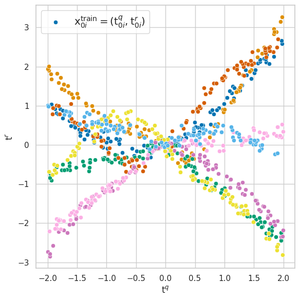
(a) Training Datasets

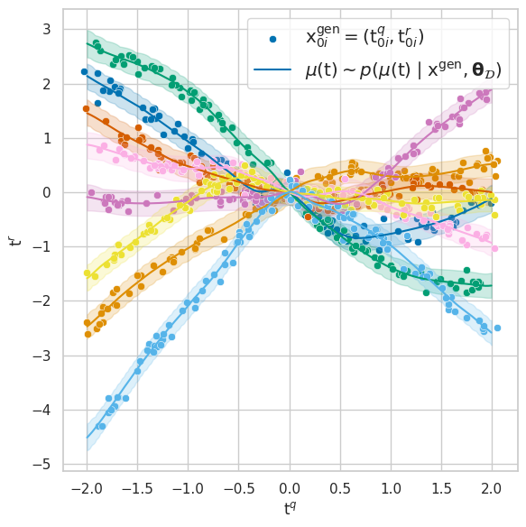
(b) Generated Datasets

Figure 11: Training and generated datasets for the synthetic regression task.

Queries $\mathrm{x}$ are sampled from a uniform distribution on [-2, 2]. Responses $\mathrm{y}$ are sampled from a normal distribution with mean $\mu(\mathrm{x})$ parameterized by a random ReLU neural network conditioned on $\mathrm{x}$ and constant standard deviation $\sigma=0.1$. We generate a set of 8000 sequences, each corresponding to a distinct random re-initialization of the neural network, with 2000 ($\mathrm{x}$, $\mathrm{y}$) examples each. Training and test data are generated over non-overlapping sets of generated sequences. Example training datasets are plotted as different colors in Figure 11.

F.2 Language

For our experiments in 3.2, we randomly sample context examples and test input/label pairs from the following datasets:

Stanford Sentiment Treebank (SST2)

SST2 [47] is a corpus with fully labeled parse trees that allows for a complete analysis of the compositional effects of sentiment in language. The corpus consists of 11,855 single sentences extracted from movie reviews. It was parsed with the Stanford parser and includes a total of 215,154 unique phrases from those parse trees, each annotated by 3 human judges. Sentiments are classified as binary labels "positive" or "negative".

Subjectivity (Subj)

The subjectivity dataset [48] contains 5,000 movie review snippets from www.rottentomatoes.com labeled "subjective", and 5,000 sentences from plot summaries available from www.imdb.com labeled "objective". Selected sentences or snippets are at least ten words long and are drawn from movies released post-2001.

Financial Phrasebank

The Financial Phrasebank dataset [81] consists of 4840 sentences from English language financial news categorized by one of 3 sentiment labels – "positive", "neutral" or "negative". The dataset is divided by agreement rate of 5-8 annotators who have been screened for sufficient business knowledge and educational background.

Hate Speech

The Hate Speech dataset [82] contains 10,568 sentences that have been extracted from Stormfront, a white supremacist forum, and are labeled as "Hate" for sentences that contain hate speech, "NoHate" for sentences that do not convey hate speech, "Relation" for consecutive sentences that collectively convey hate speech, or "Skip" for sentences not written in English or do not contain enough information to be classified as hate speech or not.

AG News

The AG News dataset [6] contains 496,835 categorized news articles from more than 2,000 news sources. The 4 largest classes (World, Sports, Business, Sci/Tech) were chosen from this corpus to construct our dataset, including only the title and description fields.

Medical Questions Pairs (MQP)

The MQP dataset [49] consists of 3,048 similar and dissimilar medical question pairs hand-generated and labeled by doctors based on patient-asked questions randomly sampled from HealthTap. Each question results in one positive question pair ("similar") that looks very different by superficial metrics, and a negative question pair ("different") that conversely look very similar, so as to ensure that the task is not trivial.

Microsoft Research Paraphrase Corpus (MRPC)

MRPC [83] consists of 5,801 pairs of sentences, each accompanied by a binary judgment indicating whether human raters considered the pair of sentences to be similar enough in meaning to be considered close paraphrases.

Recognizing Textual Entailment (RTE)

The RTE dataset [50] comes from a series of annual textual entailment challenges. Examples are constructed based on news and Wikipedia text, and labeled as binary classifications based on whether or not there is entailment.

Winograd Schema Challenge (WNLI)

The WNLI dataset [51] consists of 1,100 sentence pairs with ambiguous pronouns with different possible referents. The task is to predict if the sentence with the pronoun substituted is entailed by the original sentence.

Appendix G Additional Results

G.1 Synthetic

Figure 12 displays scatter plots of the true hallucination rate against the posterior hallucination rate over various context lengths (number of in-context examples) and values of the $\epsilon$ parameter. We can see that the trends reported Section 3.1 hold across different values for $\epsilon$.

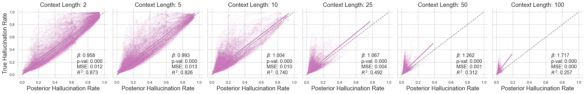
(a) $\epsilon=0.02$

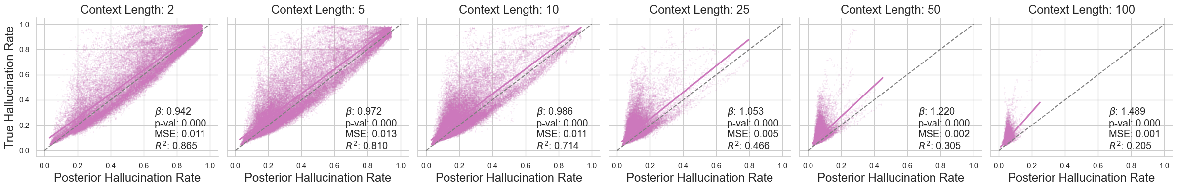
(b) $\epsilon=0.05$

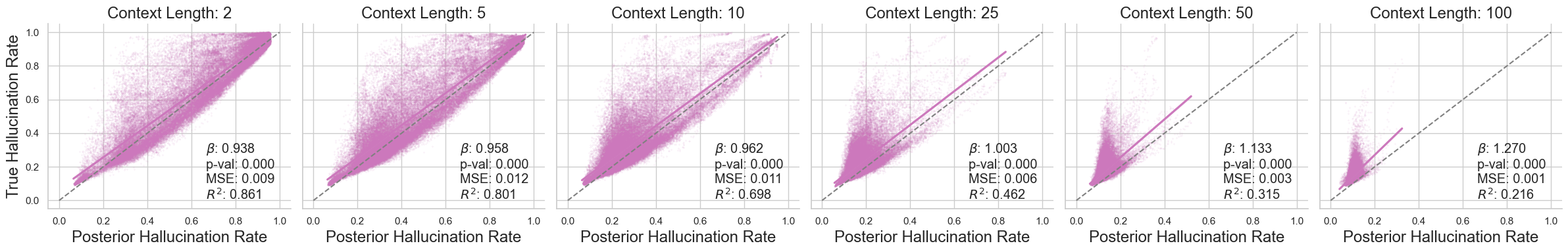
(c) $\epsilon=0.1$

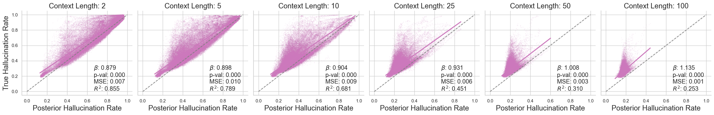
(d) $\epsilon=0.2$

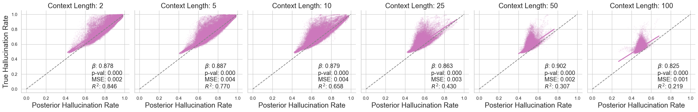
(e) $\epsilon=0.5$

Figure 12: Synthetic regression data ablation of the $\epsilon$ parameter. Scatter plots of the true hallucination rate against the posterior hallucination rate. We observe that the posterior hallucination rate is an accurate predictor of the true hallucination rate under various settings of the $\epsilon$ parameter value.

Figure 13 adds additional evidence for our reported findings and demonstrates performance over different $\epsilon$ settings.

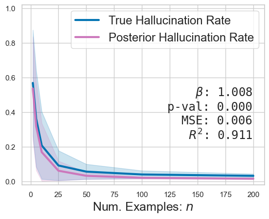
(a) $\epsilon=0.02$

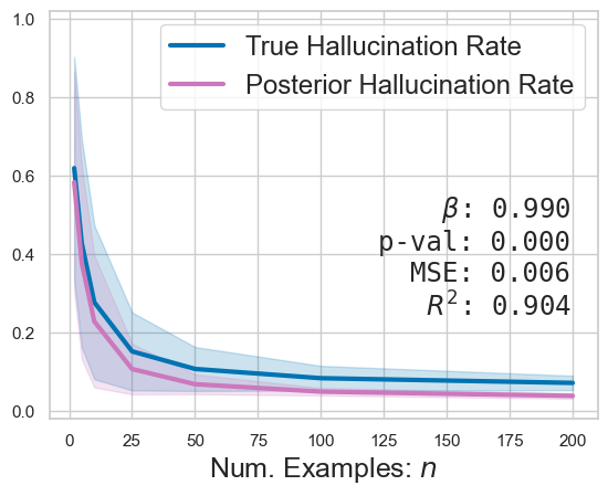
(b) $\epsilon=0.05$

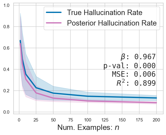
(c) $\epsilon=0.1$

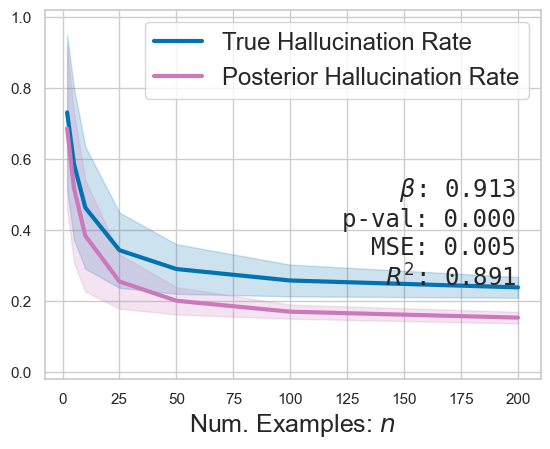
(d) $\epsilon=0.2$

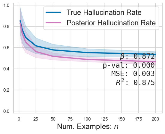
(e) $\epsilon=0.5$

Figure 13: Synthetic regression data ablation of the $\epsilon$ parameter. Plotting the true and posterior hallucination rates (THR and PHR) against the number of in-context examples ${n}$. We observe that the PHR is a good predictor of the THR across different settings of $\epsilon$. Further, we observe that the PHR is a more accurate estimator for small $\epsilon$ values than for large $\epsilon$ values.

Figure 14 shows scatter plots of the true probability of hallucination vs. the PHR under misspecified $\epsilon$ values. The THR is calculated under $\epsilon=0.05$. From top to bottom we show charts for different epsilon values, denoted as $\tilde{\epsilon}$, used to calculate the PHR. Notably, when we compare $\tilde{\epsilon}=0.1$ to $\tilde{\epsilon}=0.05$, we see that for the PHR is a more accurate predictor of the THR when the PHR is calculated with a higher $\epsilon$ value. This reflects our observation that the PHR underestimates the THR, particularly for longer context lengths (more in-context examples ${n}$).

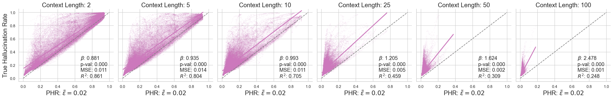
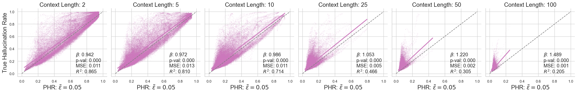
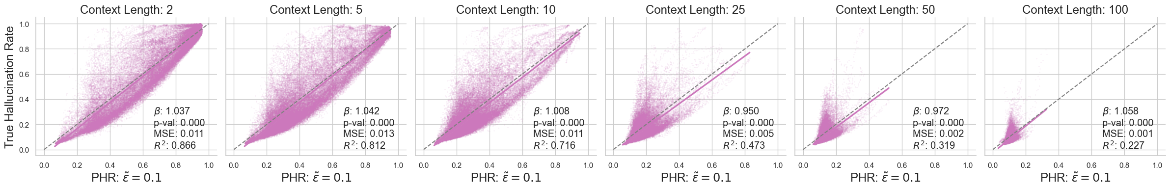
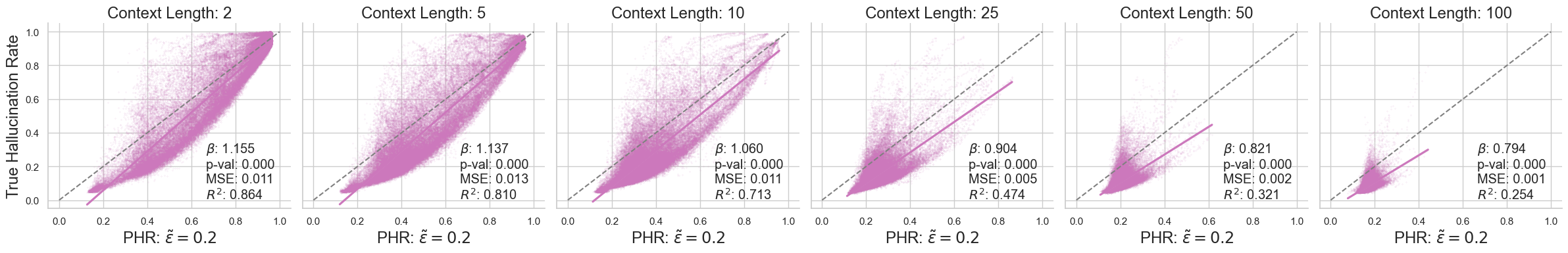
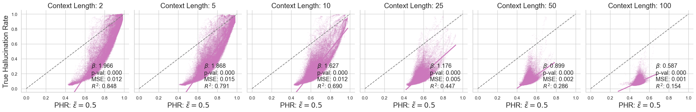
Figure 14: Synthetic data: Effect of misspecified $\epsilon$. The true value is $\epsilon=0.05$ and is used to calculate the THR. We vary the value used in calculating the posterior hallucination rate, which we denote as $\tilde{\epsilon}$ here.

Mutual information. We also evaluate the mutual information (MI) estimator ( Equation 36) as a predictor or the true hallucination rate (THR). Figure 15 shows that the MI estimates are significantly correlated with the THR, which indicates that the MI can also be an effective predictor of hallucinations. Figure 16 allows us to look deeper into the relationships between the THR, PHR, and MI. In comparing Figures 16(a) and 16(b), we see that the PHR has a more linear relationship to the THR than the MI, which has a more sigmoidal relationship to the THR. This sigmoidal relationship is amplified when plotting the PHR against the MI in Figure 16(c). This provides evidence that the PHR and MI encode the same type of information, and that the PHR is a measure of epistemic uncertainty.

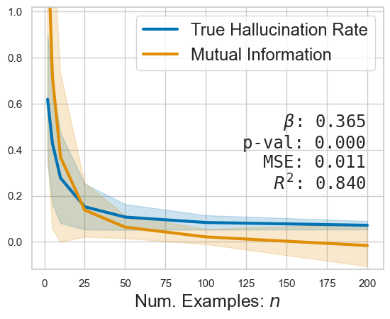
(a) MI and THR vs. ${n}$

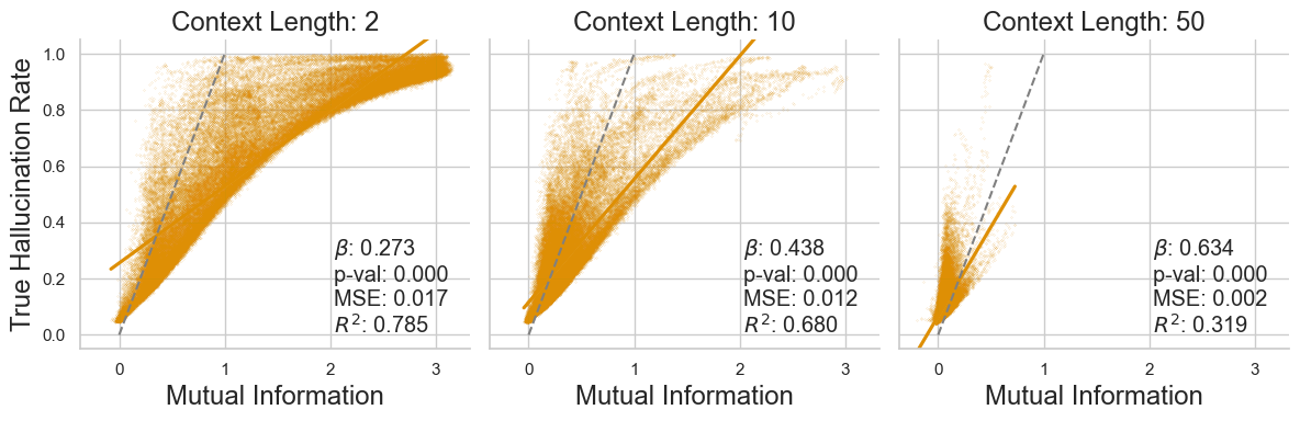
(b) Calibration: THR vs. MI against different numbers of context examples

Figure 15: Synthetic data: (a) The THR and Mutual Information reduce significantly as the number of contextual examples ${n}$ increases. (b) Calibration evaluation of the mutual information against the true probability of hallucination given $\epsilon=0.05$.

(a) THR vs. PHR

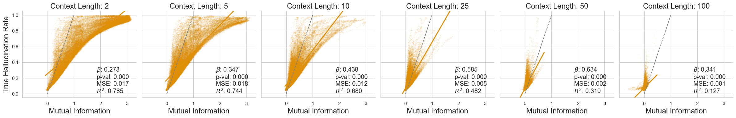
(b) THR vs. mutual information

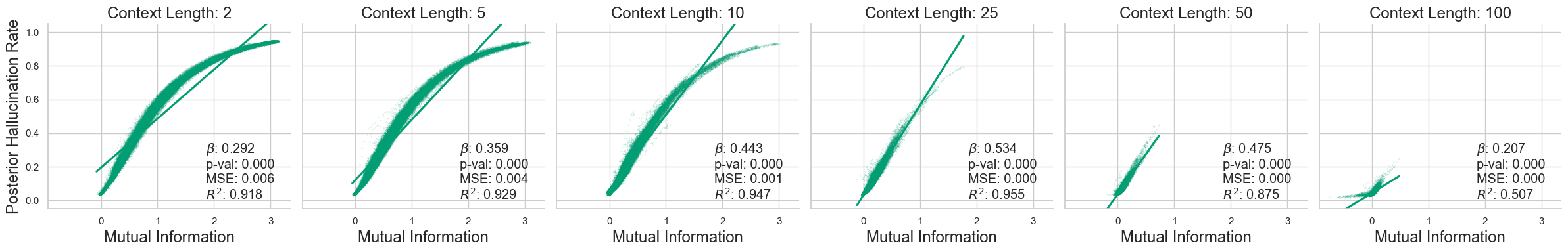
(c) PHR vs. mutual information

Figure 16: Synthetic data: visualizing and quantifying the relationship between the posterior hallucination rate and mutual information.

G.2 Language

Table 1 reports the results of an ablation study on SST2 that varies the number of generated examples, MC samples, $\mathrm{y}$ samples, and model parameters. We see that increasing the number of MC samples and number of y samples shows improvement in the $R^{2}$ scores for both MHR and the empirical error rate. Whereas increasing the number of generated samples or model size alone shows a decrease in performance on this task.

Table 1: SST2, Llama-2 ablation of hyper parameters for the posterior hallucination rate estimator

MHR		Error Rate		# Generated	# MC Samples	# $\mathrm{y}$ samples
MAE	$R^{2}$	MAE	$R^{2}$	$N-n$	$M$	$K$	# Params
0.039	0.618	0.041	0.702	5	10	50	7B
0.045	0.611	0.045	0.705	10	10	50	7B
0.039	0.618	0.041	0.702	5	10	50	7B
0.038	0.653	0.041	0.711	5	20	50	7B
0.039	0.618	0.041	0.702	5	10	50	7B
0.032	0.681	0.042	0.710	5	10	100	7B
0.039	0.618	0.041	0.702	5	10	50	7B
0.040	0.652	0.042	0.764	5	20	100	7B
0.037	0.689	0.044	0.719	10	20	100	7B
0.039	0.618	0.041	0.702	5	10	50	7B
0.033	0.607	0.041	0.669	5	10	50	13B
0.035	0.669	0.042	0.729	5	20	100	13B

Mutual Information. In Figure 19 we compare the mutual information (MI) estimator to the the error rate, model hallucination rate, and posterior hallucination rate. Figure 19(a) shows that the MI is significantly correlated with the error rate across tasks. Figure 19(b) shows that the MI is also significantly correlated with the model hallucination rate across tasks. Finally, Figure 19(c) shows the relationship between the mutual information and posterior hallucination rate across tasks and context lengths. The high $R^{2}$ value is further evidence that both estimators measure the same kind of information.

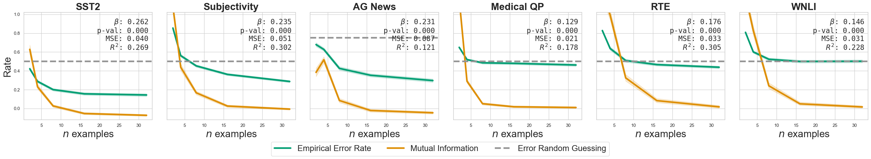
(a) Mutual information and error rate vs. $n$ examples.

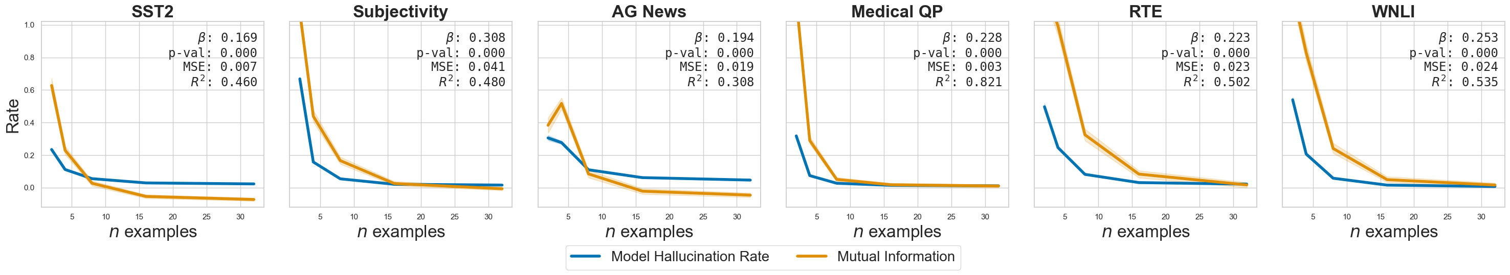
(b) Mutual information and MHR vs. $n$ examples.

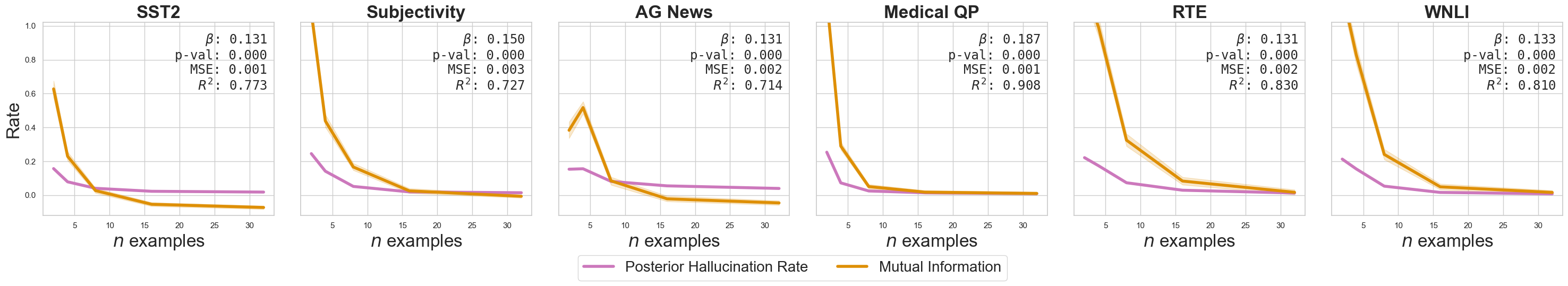
(c) Mutual information and PHR vs. $n$ examples.

Figure 19: Comparing the mutual information estimator to (a) the error rate, (b) the model hallucination rate, and (c) the posterior hallucination rate using Llama-2-7B. We see that there are significant correlations to either metric across tasks. The high $R^{2}$ between the mutual information and posterior hallucination rate is evidence that they quantify similar information.

Appendix H Computational Requirements

For our experiments, we used an internal cluster made up of A100s and RTX 8000s, which contained between 40 to 48 GBs of GPU memory. Training the models used for the synthetic experiments took about a day on one machine. For the main paper natural language results, we ran 50 seeds per dataset, where a single experiment seed took anywhere between 20 minutes and 4 hrs. We also ablated over different values of M and N (as shown in Appendix G). We ran additional experiments and developed models which required additional compute that were not included in the paper.

References

- Brown et al. [2020] Tom Brown, Benjamin Mann, Nick Ryder, Melanie Subbiah, Jared D Kaplan, Prafulla Dhariwal, Arvind Neelakantan, Pranav Shyam, Girish Sastry, Amanda Askell, et al. Language models are few-shot learners. Advances in neural information processing systems, 33:1877–1901, 2020.
- Dong et al. [2022] Qingxiu Dong, Lei Li, Damai Dai, Ce Zheng, Zhiyong Wu, Baobao Chang, Xu Sun, Jingjing Xu, and Zhifang Sui. A survey on in-context learning. arXiv preprint arXiv:2301.00234, 2022.
- Reid et al. [2024] Machel Reid, Nikolay Savinov, Denis Teplyashin, Dmitry Lepikhin, Timothy Lillicrap, Jean-baptiste Alayrac, Radu Soricut, Angeliki Lazaridou, Orhan Firat, Julian Schrittwieser, et al. Gemini 1.5: Unlocking multimodal understanding across millions of tokens of context. arXiv preprint arXiv:2403.05530, 2024.
- Ansari et al. [2024] Abdul Fatir Ansari, Lorenzo Stella, Caner Turkmen, Xiyuan Zhang, Pedro Mercado, Huibin Shen, Oleksandr Shchur, Syama Sundar Rangapuram, Sebastian Pineda Arango, Shubham Kapoor, et al. Chronos: Learning the language of time series. arXiv preprint arXiv:2403.07815, 2024.
- Maynez et al. [2020] Joshua Maynez, Shashi Narayan, Bernd Bohnet, and Ryan McDonald. On faithfulness and factuality in abstractive summarization. In Proceedings of the 58th Annual Meeting of the Association for Computational Linguistics, pages 1906–1919, Online, July 2020. Association for Computational Linguistics.
- Zhang et al. [2016] Xiang Zhang, Junbo Zhao, and Yann LeCun. Character-level convolutional networks for text classification, 2016.
- Müller et al. [2021] Samuel Müller, Noah Hollmann, Sebastian Pineda Arango, Josif Grabocka, and Frank Hutter. Transformers can do bayesian inference. In International Conference on Learning Representations, 2021.
- Xie et al. [2021] Sang Michael Xie, Aditi Raghunathan, Percy Liang, and Tengyu Ma. An explanation of in-context learning as implicit bayesian inference. In International Conference on Learning Representations, 2021.
- Feldman et al. [2023] Philip Feldman, James R Foulds, and Shimei Pan. Trapping llm hallucinations using tagged context prompts. arXiv preprint arXiv:2306.06085, 2023.
- Zhang et al. [2023a] Shuo Zhang, Liangming Pan, Junzhou Zhao, and William Yang Wang. Mitigating language model hallucination with interactive question-knowledge alignment. arXiv preprint arXiv:2305.13669, 2023a.
- Peng et al. [2023] Baolin Peng, Michel Galley, Pengcheng He, Hao Cheng, Yujia Xie, Yu Hu, Qiuyuan Huang, Lars Liden, Zhou Yu, Weizhu Chen, et al. Check your facts and try again: Improving large language models with external knowledge and automated feedback. arXiv preprint arXiv:2302.12813, 2023.
- Dziri et al. [2021] Nouha Dziri, Andrea Madotto, Osmar Zaïane, and Avishek Joey Bose. Neural path hunter: Reducing hallucination in dialogue systems via path grounding. arXiv preprint arXiv:2104.08455, 2021.
- Gao et al. [2022] Luyu Gao, Zhuyun Dai, Panupong Pasupat, Anthony Chen, Arun Tejasvi Chaganty, Yicheng Fan, Vincent Y Zhao, Ni Lao, Hongrae Lee, Da-Cheng Juan, et al. Rarr: Researching and revising what language models say, using language models. arXiv preprint arXiv:2210.08726, 2022.
- Li et al. [2023] Xingxuan Li, Ruochen Zhao, Yew Ken Chia, Bosheng Ding, Shafiq Joty, Soujanya Poria, and Lidong Bing. Chain-of-knowledge: Grounding large language models via dynamic knowledge adapting over heterogeneous sources. In The Twelfth International Conference on Learning Representations, 2023.
- Varshney et al. [2023] Neeraj Varshney, Wenlin Yao, Hongming Zhang, Jianshu Chen, and Dong Yu. A stitch in time saves nine: Detecting and mitigating hallucinations of llms by validating low-confidence generation. arXiv preprint arXiv:2307.03987, 2023.
- Su et al. [2022] Dan Su, Xiaoguang Li, Jindi Zhang, Lifeng Shang, Xin Jiang, Qun Liu, and Pascale Fung. Read before generate! faithful long form question answering with machine reading. arXiv preprint arXiv:2203.00343, 2022.
- Chuang et al. [2023] Yung-Sung Chuang, Yujia Xie, Hongyin Luo, Yoon Kim, James Glass, and Pengcheng He. Dola: Decoding by contrasting layers improves factuality in large language models. arXiv preprint arXiv:2309.03883, 2023.
- Lee et al. [2022] Nayeon Lee, Wei Ping, Peng Xu, Mostofa Patwary, Pascale N Fung, Mohammad Shoeybi, and Bryan Catanzaro. Factuality enhanced language models for open-ended text generation. Advances in Neural Information Processing Systems, 35:34586–34599, 2022.
- Shi et al. [2023] Weijia Shi, Xiaochuang Han, Mike Lewis, Yulia Tsvetkov, Luke Zettlemoyer, and Scott Wen-tau Yih. Trusting your evidence: Hallucinate less with context-aware decoding. arXiv preprint arXiv:2305.14739, 2023.
- Mielke et al. [2022] Sabrina J Mielke, Arthur Szlam, Emily Dinan, and Y-Lan Boureau. Reducing conversational agents’ overconfidence through linguistic calibration. Transactions of the Association for Computational Linguistics, 10:857–872, 2022.
- Lin et al. [2023a] Stephanie Lin, Jacob Hilton, and Owain Evans. Teaching models to express their uncertainty in words. TMLR, 2023a. URL https://arxiv.org/abs/2205.14334.
- Band et al. [2024] Neil Band, Xuechen Li, Tengyu Ma, and Tatsunori Hashimoto. Linguistic calibration of language models. arXiv preprint arXiv:2404.00474, 2024.
- Marks and Tegmark [2023] Samuel Marks and Max Tegmark. The Geometry of Truth: Emergent Linear Structure in Large Language Model Representations of True/False Datasets, 2023.
- Azaria and Mitchell [2023] Amos Azaria and Tom Mitchell. The internal state of an llm knows when it’s lying, 2023.
- Burns et al. [2022] Collin Burns, Haotian Ye, Dan Klein, and Jacob Steinhardt. Discovering latent knowledge in language models without supervision, 2022.
- Li et al. [2024] Kenneth Li, Oam Patel, Fernanda Viégas, Hanspeter Pfister, and Martin Wattenberg. Inference-time intervention: Eliciting truthful answers from a language model. Advances in Neural Information Processing Systems, 36, 2024.
- Rimsky et al. [2023] Nina Rimsky, Nick Gabrieli, Julian Schulz, Meg Tong, Evan Hubinger, and Alexander Matt Turner. Steering llama 2 via contrastive activation addition. arXiv preprint arXiv:2312.06681, 2023.
- Luo et al. [2023] Junyu Luo, Cao Xiao, and Fenglong Ma. Zero-resource hallucination prevention for large language models. arXiv preprint arXiv:2309.02654, 2023.
- Mündler et al. [2023] Niels Mündler, Jingxuan He, Slobodan Jenko, and Martin Vechev. Self-contradictory hallucinations of large language models: Evaluation, detection and mitigation. arXiv preprint arXiv:2305.15852, 2023.
- Dhuliawala et al. [2023] Shehzaad Dhuliawala, Mojtaba Komeili, Jing Xu, Roberta Raileanu, Xian Li, Asli Celikyilmaz, and Jason Weston. Chain-of-verification reduces hallucination in large language models. arXiv preprint arXiv:2309.11495, 2023.
- Zhang et al. [2019] Tianyi Zhang, Varsha Kishore, Felix Wu, Kilian Q Weinberger, and Yoav Artzi. Bertscore: Evaluating text generation with bert. In International Conference on Learning Representations, 2019.
- Kadavath et al. [2022] Saurav Kadavath, Tom Conerly, Amanda Askell, Tom Henighan, Dawn Drain, Ethan Perez, Nicholas Schiefer, Zac Hatfield Dodds, Nova DasSarma, Eli Tran-Johnson, et al. Language models (mostly) know what they know. arXiv:2207.05221, 2022. URL https://arxiv.org/abs/2207.05221.
- Kuhn et al. [2023] Lorenz Kuhn, Yarin Gal, and Sebastian Farquhar. Semantic uncertainty: Linguistic invariances for uncertainty estimation in natural language generation. arXiv preprint arXiv:2302.09664, 2023.
- Lin et al. [2023b] Zhen Lin, Shubhendu Trivedi, and Jimeng Sun. Generating with confidence: Uncertainty quantification for black-box large language models. arXiv:2305.19187, 2023b.
- Chen and Mueller [2023] Jiuhai Chen and Jonas Mueller. Quantifying uncertainty in answers from any language model and enhancing their trustworthiness. Open Review, 2023.
- Elaraby et al. [2023] Mohamed Elaraby, Mengyin Lu, Jacob Dunn, Xueying Zhang, Yu Wang, and Shizhu Liu. Halo: Estimation and reduction of hallucinations in open-source weak large language models. arXiv preprint arXiv:2308.11764, 2023.
- Manakul et al. [2023] Potsawee Manakul, Adian Liusie, and Mark JF Gales. Selfcheckgpt: Zero-resource black-box hallucination detection for generative large language models. In Conference on Empirical Methods in Natural Language Processing, 2023.
- Cole et al. [2023] Jeremy R Cole, Michael JQ Zhang, Daniel Gillick, Julian Martin Eisenschlos, Bhuwan Dhingra, and Jacob Eisenstein. Selectively answering ambiguous questions. Conference on Empirical Methods in Natural Language Processing, 2023.
- Fong et al. [2023] Edwin Fong, Chris Holmes, and Stephen G Walker. Martingale posterior distributions. Journal of the Royal Statistical Society Series B: Statistical Methodology, 85(5):1357–1391, 2023.
- Lee et al. [2023] Hyungi Lee, Eunggu Yun, Giung Nam, E Fong, and Juho Lee. Martingale posterior neural processes. In The Eleventh International Conference on Learning Representations. International Conference on Learning Representations, 2023.
- Falck et al. [2024] Fabian Falck, Ziyu Wang, and Chris Holmes. Is in-context learning in large language models bayesian? a martingale perspective. arXiv preprint arXiv:2406.00793, 2024.
- Touvron et al. [2023] Hugo Touvron, Louis Martin, Kevin Stone, Peter Albert, Amjad Almahairi, Yasmine Babaei, Nikolay Bashlykov, Soumya Batra, Prajjwal Bhargava, Shruti Bhosale, et al. Llama 2: Open foundation and fine-tuned chat models. arXiv preprint arXiv:2307.09288, 2023.
- Vaswani et al. [2017] Ashish Vaswani, Noam Shazeer, Niki Parmar, Jakob Uszkoreit, Llion Jones, Aidan N Gomez, Łukasz Kaiser, and Illia Polosukhin. Attention is all you need. Advances in neural information processing systems, 30, 2017.
- Hewitt and Savage [1955] Edwin Shields Hewitt and Leonard J. Savage. Symmetric measures on cartesian products. Transactions of the American Mathematical Society, 80:470–501, 1955. URL https://api.semanticscholar.org/CorpusID:53585081.
- Doob [1949] Joseph L Doob. Application of the theory of martingales. Le calcul des probabilites et ses applications, pages 23–27, 1949.
- Garnelo et al. [2018a] Marta Garnelo, Dan Rosenbaum, Christopher Maddison, Tiago Ramalho, David Saxton, Murray Shanahan, Yee Whye Teh, Danilo Rezende, and SM Ali Eslami. Conditional neural processes. In International conference on machine learning, pages 1704–1713. PMLR, 2018a.
- Socher et al. [2013] Richard Socher, Alex Perelygin, Jean Wu, Jason Chuang, Christopher D. Manning, Andrew Ng, and Christopher Potts. Recursive deep models for semantic compositionality over a sentiment treebank. In David Yarowsky, Timothy Baldwin, Anna Korhonen, Karen Livescu, and Steven Bethard, editors, Proceedings of the 2013 Conference on Empirical Methods in Natural Language Processing, pages 1631–1642, Seattle, Washington, USA, October 2013. Association for Computational Linguistics. URL https://aclanthology.org/D13-1170.
- Wang and Manning [2012] Sida Wang and Christopher D. Manning. Baselines and bigrams: simple, good sentiment and topic classification. In Proceedings of the 50th Annual Meeting of the Association for Computational Linguistics: Short Papers - Volume 2, ACL ’12, page 90–94, USA, 2012. Association for Computational Linguistics.
- McCreery et al. [2020] Clara H. McCreery, Namit Katariya, Anitha Kannan, Manish Chablani, and Xavier Amatriain. Effective transfer learning for identifying similar questions: Matching user questions to covid-19 faqs, 2020.
- Dagan et al. [2006] Ido Dagan, Oren Glickman, and Bernardo Magnini. The pascal recognising textual entailment challenge. In Joaquin Quiñonero-Candela, Ido Dagan, Bernardo Magnini, and Florence d’Alché Buc, editors, Machine Learning Challenges. Evaluating Predictive Uncertainty, Visual Object Classification, and Recognising Tectual Entailment, pages 177–190, Berlin, Heidelberg, 2006. Springer Berlin Heidelberg. ISBN 978-3-540-33428-6.
- Levesque et al. [2012] Hector J. Levesque, Ernest Davis, and Leora Morgenstern. The winograd schema challenge. In Gerhard Brewka, Thomas Eiter, and Sheila A. McIlraith, editors, KR. AAAI Press, 2012. ISBN 978-1-57735-560-1. URL http://dblp.uni-trier.de/db/conf/kr/kr2012.html#LevesqueDM12.
- Huszár [2023] Ferenc Huszár. Implicit bayesian inference in large language models, 2023. URL https://www.inference.vc/implicit-bayesian-inference-in-sequence-models/. [Online; accessed 10-July-2023].
- Hahn and Goyal [2023] Michael Hahn and Navin Goyal. A theory of emergent in-context learning as implicit structure induction. arXiv:2303.07971, 2023. URL https://arxiv.org/abs/2303.07971.
- Jiang [2023] Hui Jiang. A latent space theory for emergent abilities in large language models. arXiv:2304.09960, 2023. URL https://arxiv.org/abs/2304.09960.
- Zhang et al. [2023b] Yufeng Zhang, Fengzhuo Zhang, Zhuoran Yang, and Zhaoran Wang. What and how does in-context learning learn? bayesian model averaging, parameterization, and generalization. arXiv:2305.19420, 2023b. URL https://arxiv.org/abs/2305.19420.
- Von Oswald et al. [2023] Johannes Von Oswald, Eyvind Niklasson, Ettore Randazzo, João Sacramento, Alexander Mordvintsev, Andrey Zhmoginov, and Max Vladymyrov. Transformers learn in-context by gradient descent. In International Conference on Machine Learning, 2023. URL https://arxiv.org/abs/2212.07677.
- Akyürek et al. [2023] Ekin Akyürek, Dale Schuurmans, Jacob Andreas, Tengyu Ma, and Denny Zhou. What learning algorithm is in-context learning? investigations with linear models. In International Conference on Learning Representations, 2023. URL https://arxiv.org/abs/2211.15661.
- Han et al. [2023] Chi Han, Ziqi Wang, Han Zhao, and Heng Ji. In-context learning of large language models explained as kernel regression. arXiv:2305.12766, 2023. URL https://arxiv.org/abs/2305.12766.
- Hendel et al. [2023] Roee Hendel, Mor Geva, and Amir Globerson. In-context learning creates task vectors. In Findings of the Association for Computational Linguistics: EMNLP, 2023.
- Todd et al. [2024] Eric Todd, Millicent L Li, Arnab Sen Sharma, Aaron Mueller, Byron C Wallace, and David Bau. Function vectors in large language models. In International Conference on Learning Representations, 2024.
- Liu et al. [2022] Jiachang Liu, Dinghan Shen, Yizhe Zhang, Bill Dolan, Lawrence Carin, and Weizhu Chen. What makes good in-context examples for gpt-? In Proceedings of Deep Learning Inside Out (DeeLIO 2022): The 3rd Workshop on Knowledge Extraction and Integration for Deep Learning Architectures, 2022. URL https://arxiv.org/abs/2101.06804.
- Lu et al. [2022] Yao Lu, Max Bartolo, Alastair Moore, Sebastian Riedel, and Pontus Stenetorp. Fantastically ordered prompts and where to find them: Overcoming few-shot prompt order sensitivity. In ACL, 2022. URL https://arxiv.org/abs/2104.08786.
- Zhao et al. [2021] Zihao Zhao, Eric Wallace, Shi Feng, Dan Klein, and Sameer Singh. Calibrate before use: Improving few-shot performance of language models. In ICML, 2021. URL https://arxiv.org/abs/2102.09690.
- Kossen et al. [2024] Jannik Kossen, Yarin Gal, and Tom Rainforth. In-context learning learns label relationships but is not conventional learning. In The Twelfth International Conference on Learning Representations, 2024.
- Wei et al. [2023] Jerry Wei, Jason Wei, Yi Tay, Dustin Tran, Albert Webson, Yifeng Lu, Xinyun Chen, Hanxiao Liu, Da Huang, Denny Zhou, et al. Larger language models do in-context learning differently. arXiv:2303.03846, 2023. URL https://arxiv.org/abs/2303.03846.
- Razeghi et al. [2022] Yasaman Razeghi, Robert L Logan IV, Matt Gardner, and Sameer Singh. Impact of pretraining term frequencies on few-shot reasoning. In EMNLP, 2022. URL https://arxiv.org/abs/2202.07206.
- Pan et al. [2023] Jane Pan, Tianyu Gao, Howard Chen, and Danqi Chen. What in-context learning "learns" in-context: Disentangling task recognition and task learning. In ACL, 2023. URL https://arxiv.org/abs/2305.09731.
- Agarwal et al. [2024] Rishabh Agarwal, Avi Singh, Lei M Zhang, Bernd Bohnet, Stephanie Chan, Ankesh Anand, Zaheer Abbas, Azade Nova, John D Co-Reyes, Eric Chu, et al. Many-shot in-context learning. arXiv:2404.11018, 2024.
- OpenAI [2023] OpenAI. Gpt-4 technical report. 2023.
- Duan et al. [2023] Jinhao Duan, Hao Cheng, Shiqi Wang, Chenan Wang, Alex Zavalny, Renjing Xu, Bhavya Kailkhura, and Kaidi Xu. Shifting attention to relevance: Towards the uncertainty estimation of large language models. arXiv preprint arXiv:2307.01379, 2023.
- Ahdritz et al. [2024] Gustaf Ahdritz, Tian Qin, Nikhil Vyas, Boaz Barak, and Benjamin L Edelman. Distinguishing the knowable from the unknowable with language models. arXiv:2402.03563, 2024.
- Johnson et al. [2024] Daniel D Johnson, Daniel Tarlow, David Duvenaud, and Chris J Maddison. Experts don’t cheat: Learning what you don’t know by predicting pairs. arXiv:2402.08733, 2024.
- Hu et al. [2024] Zhiyuan Hu, Chumin Liu, Xidong Feng, Yilun Zhao, See-Kiong Ng, Anh Tuan Luu, Junxian He, Pang Wei Koh, and Bryan Hooi. Uncertainty of thoughts: Uncertainty-aware planning enhances information seeking in large language models. arXiv:2402.03271, 2024.
- Jeon et al. [2024] Hong Jun Jeon, Jason D Lee, Qi Lei, and Benjamin Van Roy. An information-theoretic analysis of in-context learning. arXiv:2401.15530, 2024.
- Tian et al. [2023] Katherine Tian, Eric Mitchell, Huaxiu Yao, Christopher D. Manning, and Chelsea Finn. Fine-tuning language models for factuality. arXiv, 2023.
- Garnelo et al. [2018b] Marta Garnelo, Jonathan Schwarz, Dan Rosenbaum, Fabio Viola, Danilo J Rezende, SM Eslami, and Yee Whye Teh. Neural processes. arXiv preprint arXiv:1807.01622, 2018b.
- Kim et al. [2019] Hyunjik Kim, Andriy Mnih, Jonathan Schwarz, Marta Garnelo, Ali Eslami, Dan Rosenbaum, Oriol Vinyals, and Yee Whye Teh. Attentive neural processes. In International Conference on Learning Representations, 2019.
- Nguyen and Grover [2022] Tung Nguyen and Aditya Grover. Transformer neural processes: Uncertainty-aware meta learning via sequence modeling. In International Conference on Machine Learning, 2022.
- Wei et al. [2022] Jason Wei, Xuezhi Wang, Dale Schuurmans, Maarten Bosma, Fei Xia, Ed Chi, Quoc V Le, Denny Zhou, et al. Chain-of-thought prompting elicits reasoning in large language models. Advances in neural information processing systems, 35:24824–24837, 2022.
- Loshchilov and Hutter [2019] Ilya Loshchilov and Frank Hutter. Decoupled weight decay regularization, 2019.
- Malo et al. [2013] Pekka Malo, Ankur Sinha, Pyry Takala, Pekka Korhonen, and Jyrki Wallenius. Good debt or bad debt: Detecting semantic orientations in economic texts, 2013.
- de Gibert et al. [2018] Ona de Gibert, Naiara Perez, Aitor García-Pablos, and Montse Cuadros. Hate speech dataset from a white supremacy forum. In Darja Fišer, Ruihong Huang, Vinodkumar Prabhakaran, Rob Voigt, Zeerak Waseem, and Jacqueline Wernimont, editors, Proceedings of the 2nd Workshop on Abusive Language Online (ALW2), pages 11–20, Brussels, Belgium, October 2018. Association for Computational Linguistics. doi: 10.18653/v1/W18-5102. URL https://aclanthology.org/W18-5102.
- Dolan and Brockett [2005] William B. Dolan and Chris Brockett. Automatically constructing a corpus of sentential paraphrases. In Proceedings of the Third International Workshop on Paraphrasing (IWP2005), 2005. URL https://aclanthology.org/I05-5002.