Reserve Provision from Electric Vehicles: Aggregate Boundaries and Stochastic Model Predictive Control

Abstract

Controlled charging of electric vehicles, EVs, is a major potential source of flexibility to facilitate the integration of variable renewable energy and reduce the need for stationary energy storage. To offer system services from EVs, fleet aggregators must address the uncertainty of individual driving and charging behaviour. This paper introduces a means of forecasting the service volume available from EVs by considering several EV batteries as one conceptual battery with aggregate power and energy boundaries. This avoids the impossible task of predicting individual driving behaviour by taking advantage of the law of large numbers. The forecastability of the boundaries is demonstrated in a multiple linear regression model which achieves an R² of 0.7 for a fleet of 1,000 EVs. A two-stage stochastic model predictive control algorithm is used to schedule reserve services on a day-ahead basis addressing risk trade-offs by including Conditional Value-at-Risk in the objective function. A case study with 1.2 million domestic EV charge records from Great Britain shows that increasing fleet size improves prediction accuracy, thereby increasing reserve revenues and decreasing effective charging costs. For fleet sizes of 400 or above, charging cost reductions plateau at 60%, with an average of 1.8kW of reserve provided per vehicle.

Nomenclature

Abbreviations

V2G

Vehicle-to-grid

G2V

Grid-to-vehicle

V2V

Vehicle-to-vehicle

SOC

State of Charge

MLR

Multiple Linear Regression

CVaR

Conditional Value-at-Risk

VaR

Value-at-Risk

SMPC

Stochastic Model Predictive Control

MILP

Mixed-Integer Linear Programming

Indices/Sets

$i$/$I$

Index/Set of EVs in an EV fleet

$t$/$T$

Index/Set of settlements in a planning window

$s$/$S$

Index/Set of scenarios

$j$/$J$

Index/Set of charging events at a single charger

Parameters and Variables

$\Delta t$

Settlement period duration

$\Delta t_{r}$

Maximum duration of reserve activation

$\eta$

Charging efficiency

$p^{max}$

Rated charging power in $kW$

$e^{a}$

Energy level in EV battery on arrival in $kWh$

$e^{max}$

Maximum energy capacity of EV battery in $kWh$

$e^{d}$

Expected energy in EV battery upon departure in $kWh$

$e^{min}$

Minimum allowed energy level in EV battery in $kWh$

$t_{i}^{a}$/$t_{i}^{d}$

Plug-in/plug-out time of EV $i$

$E^{u}_{t}$/$E^{l}_{t}$

Upper/lower aggregate energy boundary in $kWh$

$P^{b}_{t}$

Aggregate Power Boundary in $kW$

$E^{d}_{t}$

Difference between energy boundaries in $kWh$

$E^{EV}_{t}$

Aggregate charging trajectory in $kWh$

$P^{NR,g}_{t}$

Negative reserve power on grid side in $kW$

$P^{PR,g}_{t}$

Positive reserve power on grid side in $kW$

$P^{NR,v}_{t}$

Negative reserve power on vehicle side in $kW$

$P^{PR,v}_{t}$

Positive reserve power on vehicle side in $kW$

$P^{V2G,g}_{t}$

Vehicle-to-grid power in $kW$

$P^{G2V,g}_{t}$

Grid-to-vehicle power in $kW$

$\Delta P^{pen}$

Non-delivered power in $kW$

$C^{cha}_{s}$

Charging costs in scenario $s$ in $\pounds$

$C^{pen}_{s}$

Penalty payment in scenario $s$ in $\pounds$

$R^{res}$

Revenue from reserve provision in $\pounds$

$c^{PR}_{t}$/$c^{NR}_{t}$

Reward for providing positive/negative reserve in $\pounds/kW$

$c^{E}_{t}$

Cost of charging in $\pounds/kWh$

$z$

Number of settlements considered in baselining

$b^{PR}_{t}/b^{NR}_{t}$

Binary reserve commitment variable

$M_{1},M_{2}$

Large constants to ensure constraints are non-limiting

$p_{s}$

Probability of scenario $s$

$\Omega$

Risk aversion factor

$\alpha$

CVaR probability threshold

$w_{s}$

Auxiliary variable to derive CVaR from VaR

$\beta_{m,t}$

Regression coefficients

$H_{t}$

Temperature at time $t$ in $\degree C$

$W_{t}$

Precipitation at time $t$ in $mm$

$B_{t}$

Binary variable for bank holidays

$D_{t}$

Categorical variable for the day of the week

$\varepsilon_{t}$

Random regression error

I Introduction

Electric vehicles (EVs) are set to play a key role in the energy transition. Not only are they potentially a zero-carbon option for individual transport, but their batteries also offer the possibility of providing flexibility services to a decarbonised grid. It is predicted that by 2030, the battery capacity installed in EVs will be more than eight times the global capacity of stationary battery storage [1]. With the rise of variable renewable energy (VRE) leading to large investments in energy storage, the use of EV battery capacity for grid services could reduce system costs and provide revenue to consumers. The benefits of so-called demand response (DR) from consumer-owned equipment have been laid out clearly [2] but the uptake of DR, so far, has disappointed previous predictions [3]. The global rise of EVs now presents new possibilities for DR because these are large loads and can be manipulated with little or no interference with consumers’ lives. Further, the possibility of feeding power back from vehicle-to-grid (V2G) yields a larger volume of DR.

Consumer behaviour, however, remains inherently uncertain, and this complicates the introduction of grid services, such as frequency regulation or reserve, from EV charging. Undisrupted consumer behaviour is nearly impossible to predict at an individual level [4], but aggregate consumer behaviour, on the other hand, can be predicted with some level of certainty, even when there is little knowledge about individual behaviour [5]. This leads to considering aggregate measures of the available flexibility of an EV fleet which would facilitate both service scheduling and optimised charging so that consumers earn revenue for the former and reduce costs through the latter. It remains important to provide grid services while causing the least possible disruption to the consumer’s everyday life [6].

A number of deterministic models have been proposed to create aggregate measures of flexible charging characteristics [7, 8, 9, 10] with the stated objective of computational efficiency. [11] compares how well these models can be integrated into wider energy system models where computational efficiency is at a premium. However, none of the compared studies investigates how their aggregate models can be used to create accurate stochastic predictions for EV scheduling. Instead, a separate body of literature considers stochastic scheduling algorithms for individual EVs to deal with uncertain driving and charging behaviour [12]. [13] proposed an algorithm based on downside risk constraints (DRC) and [14] used a hybrid approach between stochastic programming and information gap decision theory (IGDT). [15] and [16] proposed stochastic optimisation approaches with the first considering V2G charging whereas the latter only studied uni-directional flexible charging. [17] and [18] considered uncertain future energy and service prices stochastically but did not treat driving behaviour as uncertain. Stochastic programming has also been used to schedule electric bus charging [19] and to schedule EV charging in the context of a virtual power plant with a range of distributed energy resources [20]. All of the listed stochastic approaches considered charging uncertainty on an individual EV level, though, and none of them took advantage of the law of large numbers to inform their scenario predictions. Aggregating the charging behaviour can reduce uncertainty and thereby increase revenue from ancillary service provision.

[21] is the only paper found that has added stochasticity to an aggregate model ([8]), and there are, to the best of the authors’ knowledge, no studies that attempt to forecast the charging characteristics from any of the aggregation models [8, 9, 10]. This paper addresses that gap by combining aggregate models and stochastic scheduling and builds a prediction model for the boundaries from [8]. The resulting scenarios are then used in stochastic model predictive control (SMPC). It is expected that aggregation of many EVs makes their charging characteristics predictable and SMPC will facilitate realisable offers of grid services. The model from [8] was chosen over other aggregation models because its aggregate boundary approach remarkably allows all of the charging characteristics of an EV fleet to be summarised into only three variables. These result from the authors considering the batteries within an EV fleet to behave like one aggregate battery. Charging and discharging this virtual battery is constrained by a power boundary, while the battery capacity is constrained by an upper and a lower energy boundary. This reduction means that the model allows for NP-hard scheduling algorithms to be deployed regardless of EV fleet size. Furthermore, their proposed aggregate energy and power boundaries are well-suited to create aggregate predictions because they allow the law of large numbers to be applied to flexible charging. The formulation of the aggregate boundaries from [8] is revisited in this paper with important extensions introduced to reflect the effect of battery cell voltage on available charging power.

This paper goes beyond the contribution of [21] by considering ancillary service provision alongside wholesale trading. Additionally, this paper investigates the predictability of the aggregate boundaries, rather than using assumed distributions, giving a realistic image of the algorithm’s performance and offering valuable insights into the effect of fleet size. The detailed contributions of this paper are:

1. The aggregation procedure from [8] is extended to explain the need for flexible V2V charging and account is taken of charge power variation with SOC.

2. The proposed aggregate energy and power boundaries are tested for their forecastability with the introduction of a multiple linear regression (MLR) model.

3. Scenarios from the MLR model are combined with a two-stage stochastic optimisation to form a stochastic model predictive control (SMPC) approach which combines ancillary service scheduling and real-time charge allocation. Conditional Value-at-Risk (CVaR) is included in the objective function as a risk measure to trade-off between additional service revenue and non-delivery penalties.

4. The predictive and financial performance of the proposed algorithm is assessed in a case study on providing reserve services in the GB electricity grid, yielding an estimation of the EV fleet size required for the realistic provision of services.

The remainder of the paper is structured as follows: Section II reintroduces the aggregate boundaries, and section III introduces the SMPC model including the MLR prediction method. Section IV demonstrates the new model in a case study on reserve services for the GB electricity system, the results of which are presented in section V.

II Energy and Power Boundaries of Aggregate Energy Storage

II-A Aggregation Procedure

The proposed aggregation treats the fleet of charging EVs as one large virtual battery but with the characteristics of that battery expressed in stochastic terms to reflect the uncertainty of the arrival and departure times of vehicles at charging points. As shown by [8], the charging behaviour of an aggregate battery can be expressed through upper and lower energy boundaries and a power boundary. The maximal charge that can be added to the aggregate battery at a point in time is limited by the upper energy boundary which is set by the amount of energy that the connected EVs can accept. The minimal amount of energy that has to be present in the aggregate battery is the lower energy boundary which is set by the required pre-departure energy of the vehicles and the energy present in newly arriving EVs. The power boundary is the sum of the rated power of all the chargers with an EV currently connected.

Figure 1 shows the boundaries applied to a single EV. The power boundary has a negative side if the charger can return power to the grid for V2G purposes and, in this figure, the positive and negative power boundaries have the same magnitude.

()/2   ()/2.2

Figure 1: Power and Energy Boundaries for an Individual EV

For an EV battery, all boundaries depend on the plug-in, or arrival ($t^{a}$) and plug-out, or departure, ($t^{d}$) times of the EV. The energy boundaries are also affected by the available power because changes in energy cannot be achieved instantaneously. The existence of the energy boundary does not render the power boundaries superfluous because they still constrain the charging trajectory within the energy boundaries. Charging can be constrained solely by the shown boundaries, so any charging trajectory that stays between the two energy boundaries and respects the power boundary should be physically possible and would ensure that departing EVs leave with the requested amount of energy ($e^{d}$). To create aggregate boundaries for multiple EVs with different charging schedules and parameters, the individual boundaries are simply stacked on top of each other. Arrival and departure times for an exemplary EV fleet are shown in Figure 2 with the corresponding boundaries displayed in Figure 3.

As with the individual boundaries, the aggregate boundaries ensure that any compliant charging trajectory honours the physical limitations of each battery and charger while ensuring each battery is fully charged upon departure (note that for simplification it is assumed throughout the rest of this paper that drivers expect their battery to be charged fully upon departure: $e^{d}=e^{max}$). The aggregation procedure can therefore summarise the driving and charging characteristics of any number of EVs into three constraining variables.

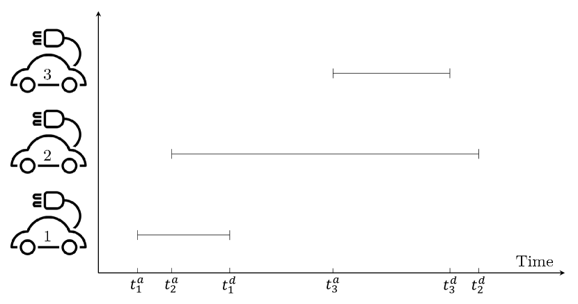
Figure 2: Arrival and Departure Times for an Example EV Fleet of 3 Vehicles

()/2   ()/2

Figure 3: Power and Energy Boundaries for Example EV Fleet from Figure 2, Including a Possible Charging Trajectory (Black Dashed Line)

II-B V2V Requirement

While any charging trajectory within the boundaries is possible, this only applies under one important assumption: the plugged-in cars are able to transfer electrical energy from vehicle to vehicle (V2V). The reason is that the energy boundaries only ensure that, before the departure of a vehicle, enough energy is present in the virtual battery to charge the departing vehicle. They do not dictate when this energy is charged to the virtual battery. It may be that the virtual battery is charged ahead of a vehicle arriving and the charge is transferred to that vehicle from another vehicle after its arrival. This is demonstrated by the example charging trajectory in Figure 3 which shows no power is delivered to the virtual battery between the arrival and departure of vehicle 3. To fulfil the charging requested by vehicle 3, vehicle 2 has previously acquired that energy and later transferred it to vehicle 3 via a V2V exchange.

V2V is a realistic possibility, even for distributed fleets, as long as chargers are physically capable of bidirectional charging but several issues need consideration such as power flow limitations, the required communications, the revenue transactions, and safety [22]. It is important to note that an aggregate battery that exploits V2V to obtain greater flexibility, as advocated by [8], incurs some power losses and perhaps use-of-system charges for the grid. Note that allowing the use of V2V averts the need for the additional constraints noted by [11] that reintroduce consideration of individual EVs into the aggregate model and thereby annul its simplification.

II-C SOC-related Power Fluctuations

The power with which an EV can be charged is often reduced as the battery approaches full charge and its cell’s voltages beging to rise [23]. This is illustrated in figure 4 which also shows how these fluctuations in charging power capability can be approximated by simply dividing the charging process into two steps.

()/5*3   ()/5*2

Figure 4: Approximation of charging power variation with SOC

For the last 20% of SOC, the approximation is that the battery can charge with only half of the average charging power. It would not make sense to use these final 20% portions for flexible charging as it would take much longer to charge them than to discharge them. Simultaneously, long-lasting high SOCs are found to be harmful to battery health [24, 25, 26] and it therefore makes sense to leave the slower-charging last 20% until the end of the charging process anyway. As such, the approximation of available power from Figure 4 can be accommodated in the aggregate boundary model by simply finishing the flexible charging window earlier and assuming direct charging for the final 20%. The resulting individual boundaries for this are shown in Figure 5. Note, that the direct charging interval, which is denoted by the two boundaries taking the same value, is not included in the aggregation procedure. Naturally, the direct charging intervals cannot be used for flexible charging.

()/2   ()/2

Figure 5: Individual EV Power and Energy Boundaries with Direct Charging at the End

III Stochastic Model Predictive Control

The aggregate boundaries permit the assessment of the potential for flexible charging from an EV fleet but in the resesarch reported in the literature they have been deterministic, meaning they do not account for uncertainty in driving behaviour. When scheduling flexible charging for future ancillary service commitments, the availability and SOC of each vehicle will be unknown. Since the proposed boundaries are an aggregate measure and thereby converge to average behaviour, their historic evolution can be used to make predictions about their future. To account for imprecise predictions of the aggregate charging behaviour, prediction errors observed in the past are used to create a range of scenarios rather than a single prediction. Each scenario represents a possible path for the boundaries to take based on aggregate charging. The scenarios form the basis for the stochastic optimisation.

III-A Predictive Model and Scenario Generation

A multiple linear regression (MLR) model is proposed to forecast each boundary. Time-of-day was identified as the most influential predictor so a separate regression was carried out for each settlement period in the day.

$$E^{u}_{t}=\beta_{0,t}+\beta_{1,t}E^{d}_{t=0}+\beta_{2,t}H_{t}+\beta_{3,t}W_{t}+\beta_{4,t}B_{t}+\beta_{5,t}D_{t}+\varepsilon_{t}$$ (1)

Equation 1 shows the regression equation for the upper energy boundary and the same equation was applied to predict the power boundary. If the lower energy boundary had been forecast independently in the same way, there would likely be scenarios in which the lower boundary would have been predicted to be higher than the upper boundary. This would have led to an impossible optimisation task in that scenario because the charging trajectory always needs to stay below the upper boundary and above the lower boundary. To prevent an infeasible optimisation problem, the difference between the lower and upper energy boundary was predicted, instead of predicting the lower boundary directly. Since there should be no historical data of the difference between the upper and lower boundary being negative, all scenarios for the boundary difference ($E^{d}_{t}$) can be assumed positive, meaning that estimating the lower boundary through Equation 2 should ensure that the lower boundary is never forecast to be higher than the upper boundary.

$$E^{l}_{t}=E^{u}_{t}-E^{d}_{t}$$ (2)

Scenarios are generated by fitting a normal distribution to the residuals between predictions and training data. The resulting distribution is then split into sections with different probabilities ($p_{s}$), i.e. $p_{s}$ is the frequency with which the prediction model over- or underestimates by the amount that corresponds to that scenario. Figures 6 and 7 show some exemplary scenario predictions where each of the opaque lines represents a scenario into which the actual future boundary may fall with probability $p_{s}$.

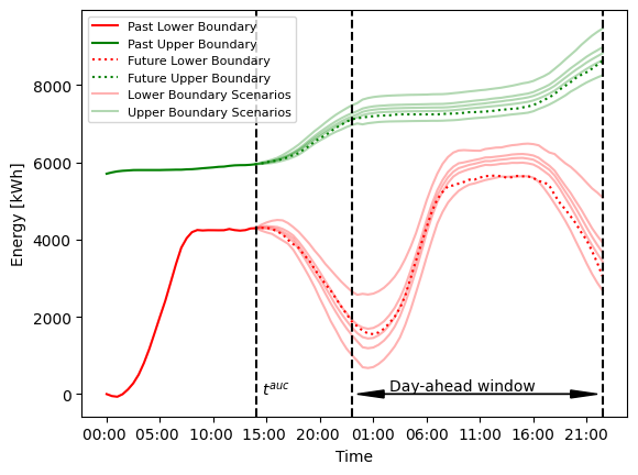
Figure 6: Predicted Scenarios for Energy Boundaries

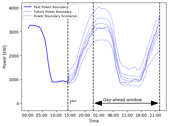
Figure 7: Predicted Scenarios for Power Boundaries

III-B Stochastic Optimisation

Model predictive control (MPC) is a control algorithm that, at each time step, optimises a process over a finite time horizon, given the future parameters by some dynamic model [27, 28]. It then implements the first time slot of the solution, repeating this process for each subsequent time interval [29]. Stochastic MPC (SMPC) adds robustness to this approach by ensuring the optimisation probabilistically considers a range of potential scenarios [30]. The procurement and execution of ancillary services (such as power reserve) in most power systems happen on two different timescales, so a two-stage SMPC is proposed here. The first stage considers the time interval in which the reserve service is procured and the second stage considers the intervals in which service commitments have been given but the charging decisions remain to be made. Procuring the reserve services carries an element of risk evaluation in that if the EV aggregator overcommits to providing a service it may incur a large penalty from the system operator for failure to deliver. A risk measure in the form of Conditional Value-at-Risk (CVaR) is introduced to control the risk aversion of the algorithm.

III-B1 Reserve bidding (First-Stage)

To effectively contract the right amount of reserve service, the algorithm has to consider the entire time window over which the services will be delivered ($t^{auc}-t^{e}$). For this time window, the proposed algorithm weighs up the revenue from reserve services ($R_{res}$) against the risk of incurring a penalty for non-delivery ($C_{pen}$). In addition, the algorithm considers the optimal charging trajectory and the resulting cost of charging ($C_{cha}$). These considerations can be formulated as a stochastic mixed-integer linear programming (MILP) optimisation:

$$\operatorname*{minimize}_{P^{PR}_{t},P^{NR}_{t},P^{G2V}_{s,t},P^{V2G}_{s,t},\Delta P^{pen}_{s,t}}\quad\sum_{s\epsilon S}p_{s}(C^{cha}_{s}+C^{pen}_{s}-A_{s})-R^{res}$$ (3)

where

$$C^{cha}_{s}=\sum^{T}_{t=0}c^{E}_{t}\left(P^{G2V,g}_{s,t}-P^{V2G,g}_{s,t}\right)\Delta t$$ (4)

$$R^{res}=\sum^{T}_{t=0}(c_{t}^{PR}P^{PR,g}_{t}+c_{t}^{NR}P^{NR,g}_{t})$$ (5)

$$C^{pen}_{s}=\sum^{T}_{t=0}c^{pen}\Delta P_{s,t}^{pen}$$ (6)

$$A_{s}=\left(\sum^{T}_{t=0}\left(P^{G2V}_{s,t}\eta-\frac{P^{V2G}_{s,t}}{\eta}\right)-E^{l}_{s,T}\right)\bar{c}^{E}$$ (7)

subject to:

$$E^{EV}_{s,t_{x}}=\sum_{t^{auc}}^{t_{x}-1}\left(P^{G2V,g}_{s,t}\eta-\frac{P^{V2G,g}_{s,t}}{\eta}\right)\Delta t+E_{t^{auc}-1}^{EV}$$ (8)

$$E^{u}_{s,t}\geq E^{EV}_{s,t}\geq E^{l}_{s,t}$$ (9)

$$\frac{P^{V2G,g}_{s,t}}{\eta}+P^{G2V,g}_{s,t}\leq P^{b}_{s,t}$$ (10)

$$P^{PR,v}_{s,t}=\frac{P^{PR,g}_{t}-\frac{1}{z}\sum^{t-1}_{t-z}(P^{G2V,g}_{s,t}-P^{V2G,g}_{s,t})}{\eta}$$ (11)

$$P^{NR,v}_{s,t}=\left(P^{NR,g}_{t}+\frac{1}{z}\sum^{t-1}_{t-z}\left(P^{G2V,g}_{s,t}-P^{V2G,g}_{s,t}\right)\right)\eta$$ (12)

$$b^{PR}_{t}\times M_{1}\geq P^{PR}_{g}$$ (13)

$$b^{NR}_{t}\times M_{1}\geq P^{NR}_{g}$$ (14)

$$E^{EV}_{s,t}-\left(P^{PR,v}_{s,t}+\frac{\Delta P_{s,t}^{pen}}{\eta}\right)\Delta t_{r}\geq E^{l}_{s,t}-(1-b^{PR}_{t})M_{2}$$ (15)

$$E^{EV}_{s,t}+(P^{NR,v}_{s,t}\eta-\Delta P_{s,t}^{pen}\eta)\Delta t_{r}\leq E^{u}_{s,t}+(1-b^{NR}_{t})M_{2}$$ (16)

$$P^{PR,v}_{s,t}-\frac{\Delta P_{s,t}^{pen}}{\eta}\leq P^{b}_{s,t}+\left(1-b^{PR}_{t}\right)M_{2}$$ (17)

$$\frac{P^{NR,v}_{s,t}}{\eta}-\Delta P_{s,t}^{pen}\leq P^{b}_{s,t}+\left(1-b^{PR}_{t}\right)M_{2}$$ (18)

Reserve revenue, charging costs and penalty payments are defined in equations (4) - (6) and equation (7) defines an ”end-of-plan credit” term ($A_{s}$) that compensates the algorithm for any energy that is left in the vehicles’ batteries at the end of the planning window. This term alleviates the need for complex cross-window relaxations as introduced by the authors of [21]. Equation (8) defines the aggregate charging trajectory as a function of power charged to and from the grid while Equations (9) - (10) ensure that this charging trajectory always stays within the energy and power boundaries. Equations (11) and (12) express the reserve power that has to be provided by the EV fleet as a function of the contracted reserve power and the baseline demand/generation from the previous $z$ time intervals. Without further adjustment, this would mean that, in the case of no reserve commitments ($P$), the fleet would be constrained to provide reserve power based on its baseline demand ($P$). Naturally, there should be no reserve constraints, if the aggregator has not committed to providing any reserve power so that a binary variable $b_{t}$ is introduced by Equations (13) and (14). $b_{t}$ that can only take the value zero if no reserve has been scheduled for that particular time interval $t$. Equations (15) and (16) ensure that a penalty is applied if the reserve commitments violate the energy boundaries and Equations (17) and (18) ensure the same for the power boundary. In the case of no reserve commitments ($b_{t}=0$), the term $(1-b_{t})M_{2}$ adds a sufficiently large number to the respective boundary to make sure it is not limiting.

III-B2 Charge Scheduling (Second-Stage)

With the reserve provision for a future time window already procured, for each time interval within that window, the algorithm simply needs to weigh up the charging costs ($C_{cha}$) and the expected cost of incurring a penalty ($C_{pen}$).

$$\operatorname*{minimize}_{P^{G2V}_{s,t},P^{V2G}_{s,t},\Delta P^{pen}_{s,t}}\quad\sum_{s\epsilon S}p_{s}(C^{cha}_{s}+C^{pen}_{s}-A_{s})\\$$ (19)

subject to: (8) - (18)

With no reserve service decisions to be made, the charge scheduling step only considers scenarios to find the optimal charging trajectory in all situations. Since the decisions in which risk aversion plays a role were already made in the first stage, the second-stage optimisation can simply have the expected value as its objective. This means that the risk measure CVaR is only applied to the first-stage optimisation.

III-B3 Conditional Value-at-Risk

The first-stage optimisation involves the commitment to provide a future service with only limited certainty that the resources to provide the service will actually be available. With the possibility of incurring prohibitively large penalties for non-delivery, this requires weighing up the risk of incurring a penalty against higher expected returns. Conventional stochastic programming optimises the expected value and thus fails to distinguish risk preferences. Conditional Value-at-Risk is a common risk measure that expresses the expected value in the $\alpha\%$ worst-case outcomes, i.e. $CVaR(\alpha=0.1)$ expresses the expected value for the worst 10% of possible outcomes. [31] introduced a methodology for including the risk measure CVaR in the objective of a stochastic programming problem while keeping the problem convex. This allows a stochastic algorithm to fine-tune its risk aversion. For our case, this is formulated following previous implementations of CVaR in a stochastic programming objective function [32, 33]:

$$\min\quad(1-\Omega)\times(C^{cha}_{s}+C^{pen}_{s}-R^{res})+\Omega\times\operatorname{CVaR}$$ (20)

subject to:

$$\operatorname{CVaR}\geq\operatorname{VaR}+\frac{1}{1+\alpha}\sum_{s\epsilon S}p_{s}w_{s}$$ (21)

$$w_{s}\geq(C^{cha}_{s}+C^{pen}_{s})-R^{res}-\operatorname{VaR}$$ (22)

and (8) - (18)

Equation (18) is the updated objective function that considers both the expected outcome and the risk measure CVaR. $\Omega$ decides the risk-aversion of the algorithm with a higher $\Omega$ increasing the weighting of $\operatorname{CVaR}$. Equations (19) - (20) constrain the $\operatorname{CVaR}$ following [31]. Additionally, the operational constraints from Equations (8) - (16) still apply. Three risk-aversion factors ($\Omega$) are considered: a risk-neutral approach ($\Omega=0$), a risk-averse approach ($\Omega=0.5$), and a least-regrets approach ($\Omega=1$) that solely focuses on the outcome in the worst case.

IV Case Study

The proposed charging algorithm was trialled in a case study on the ”Quick Reserve” product by the British system operator National Grid Electricity System Operator (NG ESO). Data and code files for the case study have been made available , and a Gurobi solver [34] was used via its Python API to solve the MILP optimisation.

IV-A NG ESO Quick Reserve Product

Quick Reserve is an ancillary service product that NG ESO planned to introduce in October 2023 although its implementation has been delayed [35]. Quick reserve will require activation periods of below 1 minute which makes it a good fit for V2G-capable EVs. The activation periods will be no longer than 15 minutes and units will be allowed a recovery period of up to 3 minutes after being activated before the units must be available again. The maximum time for which Quick Reserve could be active ($\Delta t_{r}$) in any half-an-hour settlement period is therefore 27 minutes (two activations separated by 3 minutes). The baseline against which the delivered reserve will be measured will be taken from the hour (two settlement periods) prior to activation. Reserve capacities will be auctioned every day at 2 pm for the following day, divided into 2h service windows (SW) from 11 pm until 11 pm [35]. Reserve commitments will have to be equal across four adjacent settlement periods. Quick reserve comprises both positive quick reserve ($P^{PR}$) providing power to the grid and negative quick reserve ($P^{NR}$) which is additional load to balance sudden load rejection elsewhere.

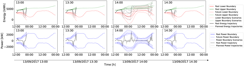
Figure 8: Illustration of SMPC Algorithm for Aggregate Energy and Power Boundaries of 720 EVs. Plans are for settlements starting 13:00 till 14:30 with day-ahead auction at 14:00

IV-B Data

IV-B1 EV charging

The UK Department for Transport [36] provides a large EV charging dataset comprising 25,000 chargers and 3.2 million charging events. For each charging event, the data includes the charger ID, plug-in time, plug-out time, and the amount of energy that was charged. The dataset does not contain information about the EV that was charging but, because only domestic chargers are included, it is assumed here that each charger serves only one vehicle and thus information from that vehicle can be inferred from the charger data. The rated power of each charger was assumed to be the maximum power that is seen to be drawn by that charger across the data set

$$p^{max}_{i}=\max\left(\frac{\Delta e_{j}}{\Delta t_{j}}|j\epsilon J\right),$$ (23)

where $J$ is the set of charging events that are completed at charger $i$. Similarly, the maximum battery capacity of each vehicle is taken as the maximum energy that is delivered to it in any charging event

$$e^{max}_{i}=\max\left(\Delta e_{j}|j\epsilon J\right).$$ (24)

Because some chargers may not have charged at their rated power, or vehicles may never have fully charged their battery in a single charge across the dataset minimum values of 7 kW and 16 kWh were set. It was also assumed that all chargers are bidirectional, which is unlikely to be the case in the actual data but was important for exploring the V2G concept. Cleansing of the raw data included the exclusion of any two overlapping charging events for the same charger ID and the exclusion of charging events that lasted for more than a week.

IV-B2 Wholesale electricity and reserve service prices

Price data for the British wholesale day-ahead market is no longer published, so the system price in the Balancing Mechanism Reporting System (BMRS) was taken as a substitute [37]. Since the Quick Reserve product has not been launched yet, price data for reserve services was adapted from the old ”Fast Reserve” product [38]. This derived Quick Reserve price data was compared with auction data from the Synchronous Reserve product in the Pennsylvania-New Jersey-Maryland (PJM) Interconnection [39] for validation. The results were a nighttime (23:00 - 07:00) reserve reward of £0.31/MW per settlement and a daytime (07:00 - 23:00) reward of £1.41/MW per settlement.

National Grid ESO states that non-delivery of ancillary services can be penalised by up to 30% of the monthly revenue [40]. Using an iterative estimation, this was found to be about £52/MW for the case study at hand.

IV-B3 Regressors in the predictive model

Two predictive variables required additional data, precipitation ($W_{t}$) and temperature ($H_{t}$), which was sourced from the respective Hadley centre datasets [41, 42]. Note that precipitation data is for England and Wales while temperature data is for central England.

V Results

V-A Illustration of Algorithm Performance

Figure 8 illustrates how the SMPC algorithm predicts scenarios and solves the resulting stochastic optimisation for every settlement period. At 13:00 and 13:30, the algorithm considers the next 9 hours (until 22:00 and 22:30 respectively) to optimise charging for that period. The algorithm considers a much longer time window at 14:00 than at other times because at this point the algorithm has to choose reserve commitments for a 24-hour period beginning at 23:00 and thus has to consider scenarios for the 33 hours ahead. With the reserve commitments for the next day decided the algorithm can then return to a 9-hour time window in the subsequent settlement (14:30).

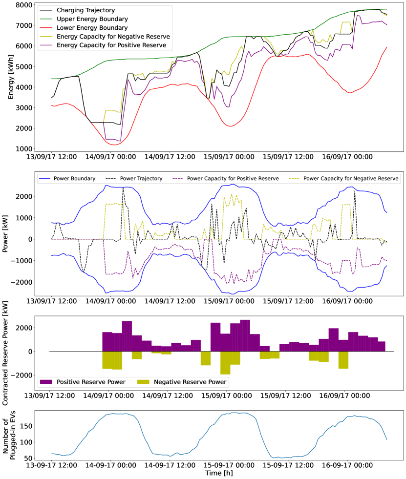
Figure 9: Illustration of Charging Trajectory and Reserve Commitments With Energy and Power Boundaries for risk-averse aggregator ($\Omega=0.5$) of a 720 EV fleet

Figure 9 shows the resulting trajectories that the process shown in Figure 8 produces. In yellow and purple, the capacity that has to be kept to service negative and positive reserve has been added to the power and energy trajectories. While these depend on the contracted reserve, shown in the third part of Figure 9, they do not simply equate because delivered reserve ($P^{PR,v}$) depends both on contracted reserve ($P^{PR,g}$) and the previous baseline as stated in Equations (11) - (12). For a given settlement, the delivered reserve is the difference between the contracted reserve and the power delivered in the two previous settlements, i.e. the baseline. Positive reserve services denote the feeding of power into the grid, reducing the energy levels in the aggregate battery. The energy capacity for positive reserve therefore falls below the charging trajectory because the aggregator has to keep sufficient energy levels to discharge positive reserve energy without reaching the lower energy boundary. Similarly, negative reserve means absorbing power from the grid, for which the aggregator has to ensure that there is sufficient ”empty” battery capacity. At times, when the aggregator schedules no reserve despite sufficient capacity, this is usually because the algorithm expects greater earnings from energy arbitrage than from reserve service provision. Also note, how the risk-averse nature of the algorithm makes it systematically schedule reserve services well below the power boundaries to ensure that the likelihood of not having enough power available stays sufficiently small.

Figure 9 also shows that the energy boundaries rarely constrain the reserve services and it is usually the power boundaries that dictate how much reserve power the algorithm can schedule. This observation is consistent throughout all results and indicates that the limiting factor for a vehicle to deliver reserve services is the charger power rather than the battery capacity. Charger infrastructure could therefore be seen as more important than battery energy management for the delivery of ancillary services via V2G.

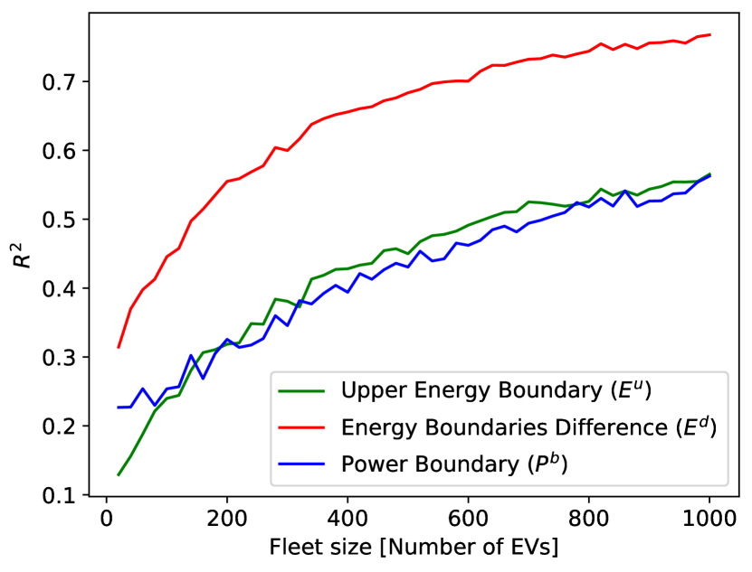
Figure 10: Coefficient of Determination ($R^{2}$) against Different Fleet Sizes

V-B Comparison of SMPC against Benchmarks

Figure 10 plots the coefficient of determination ($R^{2}$), which is the fraction of variation in a variable that is predicted by a model. It can be seen that the predictions improve with fleet size, allowing the SMPC algorithm to make more use of reserve as the number of EVs in the fleet increases. Figure 11 plots the average reserve that can be scheduled per vehicle against fleet size for 5 algorithms. Two benchmark algorithms are shown: one that, unrealistically, has perfect future knowledge ($BM_{2}$) but serves as a limit case and the other ($BM_{1}$) is a deterministic version of our model that makes a single prediction but does not account for uncertainty and makes naive predictions of reserve that risk non-delivery penalties. Three cases for the proposed SMPC algorithm are shown for different risk preferences and all three scheduled less reserve than the benchmarks because they cannot match perfect foresight and are not naive about penalties. The risk-neutral algorithm ($\Omega=0$) optimistically schedules more reserve because it is more prone to ignore the worst scenarios. With improving prediction accuracy, as shown in Figure 10, more reserve can be scheduled per vehicle but at fleet sizes beyond 250 EVs, the reserve commitment levels off which is likely because the predictions improve at a slower rate beyond that. Once a certain prediction quality has been achieved, further small prediction improvements are likely to have little impact on the algorithm’s reserve commitments as they present only small changes to the predicted scenarios.

The total cost of charging is made up of the wholesale electricity costs minus the revenues earned from reserve contracts plus any penalty for non-delivery of that service. Figure 12 plots the total cost for the risk-neutral algorithm and the two benchmarks. The perfect foresight case earns a high revenue from reserve and suffers no penalties so achieves the lowest cost. The risk-neutral SMPC case has somewhat higher costs (lower reserve revenue and some penalties) but approaches the perfect foresight case. The simple deterministic method has the highest cost because of large penalties arising from over-commitment of reserve. The costs of three different risk versions for SMPC are compared in Figure 13 and are seen to have only small differences between them. All charge at lower costs, though, than the simple case of charge-on-arrival with no services ($\sim 6p/kWh$) and all approach the perfect foresight case ($\sim 1.7p/kWh$). SMPC performance continues improving for larger fleets until a fleet size of roughly 400 is reached where the effective cost plateaus at around 2.5p/kWh, some 60% below charge-on-arrival. The reason the plateau is at 400 EVs not the 250 EVs at which per-EV reserve commitments level off, is that the incurred penalties reduce between 250 and 400 EVs due to more accurate predictions. For the stochastic algorithms, a 25% reduction in effective charging costs can be attributed to energy arbitrage with the remaining 15 - 35 percentage points being reserve service revenue. Price reductions are based on current reserve price estimations (2.09 £/MW/h) which may change due to VRE penetration [43], storage expansion [44], or market power of a single aggregator[45].

The risk-neutral algorithm has somewhat higher costs than the other two SMPC cases which is due to higher penalty payments and somewhat unexpected because the risk-neutral algorithm focuses on the expected value. One possible explanation is that the in-sample scenario generation is being used for out-of-sample predictions. This may result in the scenarios overestimating the accuracy of the predictions and thereby leading to more ”worst scenarios” materialising, disadvantaging the risk-neutral algorithm.

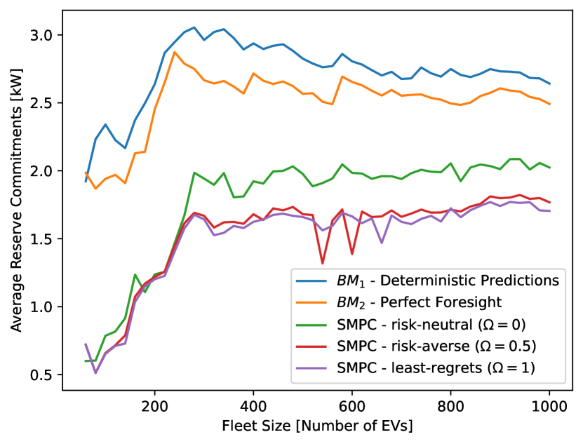
Figure 11: Average Contracted Reserve per Vehicle for Different Fleet Sizes

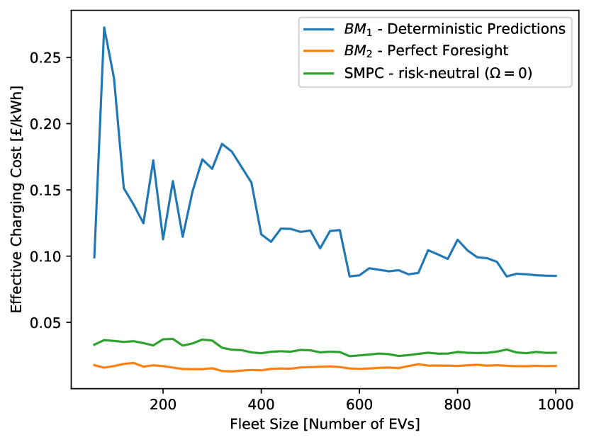
Figure 12: Effective Charging Costs ($C^{cha}+C^{pen}-R^{res}$) over Fleet Size

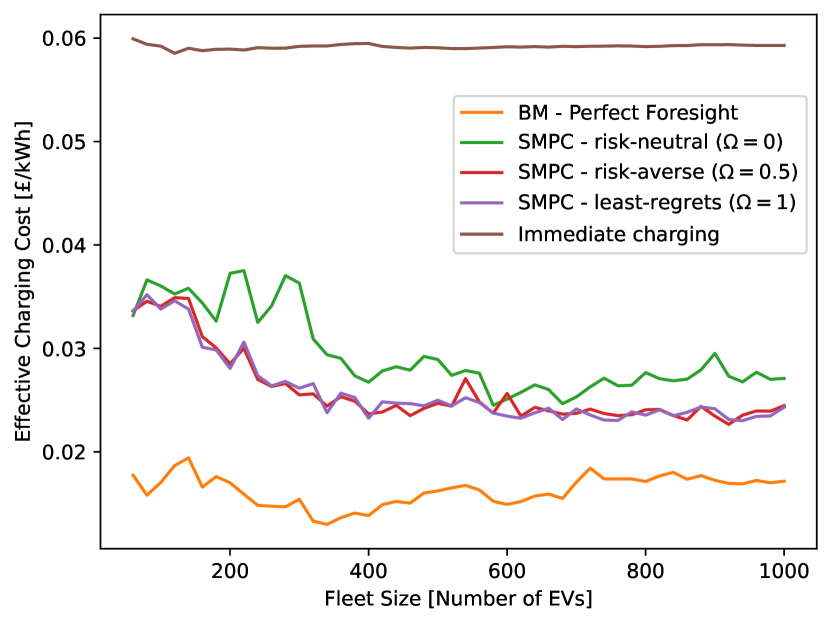
Figure 13: Effective Charging Costs For Different Risk Aversion Factors

VI Conclusion

A stochastic aggregate model for scheduling ancillary services from V2G-capable EV fleets while considering uncertain driver behaviour has been introduced. Aggregate boundaries for energy and power are used to summarise the potential flexibility of a fleet of EVs. Multiple linear regression is used to forecast the aggregate boundaries, and scenarios are generated based on historic distributions to account for prediction errors. A stochastic model predictive control algorithm is proposed that uses the scenario forecasts for day-ahead scheduling of ancillary services and includes a Conditional Value-at-Risk to ensure the algorithm does not make overly optimistic decisions that incur penalties.
A case study is carried out for reserve service provision in the GB electricity grid. Using a large dataset of domestic EV chargers, an MLR model can predict the boundaries with increasing accuracy, reaching an $R^{2}$ of 0.7, for a fleet of 1,000, meaning the uncertainty has been reduced by 70% compared to an algorithm without aggregate predictions. The revenue per EV is observed to increase as the number of EVs in the fleet increases because aggregate driving behaviour becomes more predictable. After reaching a fleet size of around 400 EVs, the increase in revenue per EV levels off. For fleet sizes above 400 EVs an average 1.8kW of reserve power is scheduled, reducing the charging costs by 60%.
The simulation results show that the proposed algorithm allows the grid operator to plan without compromising on consumer needs. So long as consumers are willing to indicate their planned departure, their vehicle battery can reliably provide grid services without any impact on their planned driving.

References

- [1] I. Staffell, “Grid security and energy storage,” 2023, 18th IAEE European conference, Milan. [Online]. Available: https://www.aiee.it/iaee_2023/wp-content/uploads/2023/08/Staffell_ppt_Milan2023plenary.pdf
- [2] G. Strbac, “Demand side management: Benefits and challenges,” Energy policy, vol. 36, no. 12, pp. 4419–4426, 2008.
- [3] M. H. J. Weck, J. van Hooff, and W. G. J. H. M. van Sark, “Review of barriers to the introduction of residential demand response: a case study in the netherlands,” International Journal of Energy Research, vol. 41, no. 6, pp. 790–816, 2017.
- [4] V. Dyo, “Behavior-neutral smart charging of plugin electric vehicles: Reinforcement learning approach,” IEEE Access, vol. 10, pp. 64 095–64 104, 2022.
- [5] B. Travacca, S. Bae, J. Wu, and S. Moura, “Stochastic day ahead load scheduling for aggregated distributed energy resources,” in 2017 IEEE Conference on Control Technology and Applications (CCTA). IEEE, 2017, pp. 2172–2179.
- [6] E. Crisostomi, R. Shorten, S. Stüdli, and F. Wirth, Electric and plug-in hybrid vehicle networks: optimization and control. CRC Press, 2017.
- [7] C. Le Floch, F. Belletti, and S. Moura, “Optimal charging of electric vehicles for load shaping: A dual-splitting framework with explicit convergence bounds,” IEEE Transactions on Transportation Electrification, vol. 2, no. 2, pp. 190–199, 2016.
- [8] H. Zhang, Z. Hu, Z. Xu, and Y. Song, “Evaluation of achievable vehicle-to-grid capacity using aggregate pev model,” IEEE Transactions on Power Systems, vol. 32, no. 1, pp. 784–794, 2017.
- [9] L. Xu, H. Ü. Yilmaz, Z. Wang, W.-R. Poganietz, and P. Jochem, “Greenhouse gas emissions of electric vehicles in europe considering different charging strategies,” Transportation Research Part D: Transport and Environment, vol. 87, p. 102534, 2020.
- [10] R. Yu, W. Zhong, S. Xie, C. Yuen, S. Gjessing, and Y. Zhang, “Balancing power demand through ev mobility in vehicle-to-grid mobile energy networks,” IEEE Transactions on Industrial Informatics, vol. 12, no. 1, pp. 79–90, 2015.
- [11] Z. Wang, P. Jochem, H. Ü. Yilmaz, and L. Xu, “Integrating vehicle-to-grid technology into energy system models: Novel methods and their impact on greenhouse gas emissions,” Journal of Industrial Ecology, vol. 26, no. 2, pp. 392–405, 2022.
- [12] N. I. Nimalsiri, C. P. Mediwaththe, E. L. Ratnam, M. Shaw, D. B. Smith, and S. K. Halgamuge, “A survey of algorithms for distributed charging control of electric vehicles in smart grid,” IEEE Transactions on Intelligent Transportation Systems, vol. 21, no. 11, pp. 4497–4515, 2019.
- [13] M.-W. Tian, S.-R. Yan, X.-X. Tian, M. Kazemi, S. Nojavan, and K. Jermsittiparsert, “Risk-involved stochastic scheduling of plug-in electric vehicles aggregator in day-ahead and reserve markets using downside risk constraints method,” Sustainable Cities and Society, vol. 55, p. 102051, 2020.
- [14] P. Aliasghari, B. Mohammadi-Ivatloo, and M. Abapour, “Risk-based scheduling strategy for electric vehicle aggregator using hybrid stochastic/igdt approach,” Journal of Cleaner Production, vol. 248, p. 119270, 2020.
- [15] Z. Wang, P. Jochem, and W. Fichtner, “A scenario-based stochastic optimization model for charging scheduling of electric vehicles under uncertainties of vehicle availability and charging demand,” Journal of Cleaner Production, vol. 254, p. 119886, 2020.
- [16] L. Gong, Y. Guo, H. Sun, and W. Deng, “Model predictive control-based real-time optimal charging of electric vehicle aggregators,” in 2022 IEEE Power & Energy Society General Meeting (PESGM). IEEE, 2022, pp. 1–5.
- [17] B. Han, S. Lu, F. Xue, and L. Jiang, “Day-ahead electric vehicle aggregator bidding strategy using stochastic programming in an uncertain reserve market,” IET Generation, Transmission & Distribution, vol. 13, no. 12, pp. 2517–2525, 2019.
- [18] S. Bae, H. Zhang, D. Wang, C. Sheppard, and S. Saxena, “Optimal bidding strategy for v2g regulation services under uncertainty,” in 2017 IEEE Power & Energy Society General Meeting, 2017, pp. 1–5.
- [19] X. Duan, Z. Hu, Y. Song, Y. Cui, and Y. Wen, “Bidding and charging scheduling optimization for the urban electric bus operator,” IEEE Transactions on Smart Grid, vol. 14, no. 1, pp. 489–501, 2023.
- [20] Z. Wang, J. Gao, R. Zhao, J. Wang, and G. Li, “Optimal bidding strategy for virtual power plants considering the feasible region of vehicle-to-grid,” Energy Conversion and Economics, vol. 1, no. 3, pp. 238–250, 2020.
- [21] Z. Bao, Z. Hu, and A. Mujeeb, “A novel electric vehicle aggregator bidding method in electricity markets considering the coupling of cross-day charging flexibility,” IEEE Transactions on Transportation Electrification, pp. 1–1, 2024.
- [22] A. Shafiqurrahman, V. Khadkikar, and A. K. Rathore, “Vehicle-to-vehicle (v2v) power transfer: Electrical and communication developments,” IEEE Transactions on Transportation Electrification, 2023.
- [23] C. McLaughlin, “Visualizing electric vehicle (ev) charging curves,” https://conormclaughlin.net/2023/02/visualizing-electric-vehicle-ev-charging-curves/, 2023, accessed: 2024-01-11.
- [24] J. Schmalstieg, S. Käbitz, M. Ecker, and D. U. Sauer, “A holistic aging model for li (nimnco) o2 based 18650 lithium-ion batteries,” Journal of Power Sources, vol. 257, pp. 325–334, 2014.
- [25] N. Collath, B. Tepe, S. Englberger, A. Jossen, and H. Hesse, “Aging aware operation of lithium-ion battery energy storage systems: A review,” Journal of Energy Storage, vol. 55, p. 105634, 2022.
- [26] J. S. Edge, S. O’Kane, R. Prosser, N. D. Kirkaldy, A. N. Patel, A. Hales, A. Ghosh, W. Ai, J. Chen, J. Yang et al., “Lithium ion battery degradation: what you need to know,” Physical Chemistry Chemical Physics, vol. 23, no. 14, pp. 8200–8221, 2021.
- [27] M. Arnold and G. Andersson, “Model predictive control of energy storage including uncertain forecasts,” in Power systems computation conference (PSCC), Stockholm, Sweden, vol. 23, 2011, pp. 24–29.
- [28] J. B. Rawlings, D. Q. Mayne, M. Diehl et al., Model predictive control: theory, computation, and design. Nob Hill Publishing Madison, WI, 2017, vol. 2.
- [29] A. Mesbah, “Stochastic model predictive control: An overview and perspectives for future research,” IEEE Control Systems Magazine, vol. 36, no. 6, pp. 30–44, 2016.
- [30] A. J. King and S. W. Wallace, Modeling with stochastic programming. Springer, 2012.
- [31] R. T. Rockafellar, S. Uryasev et al., “Optimization of conditional value-at-risk,” Journal of risk, vol. 2, pp. 21–42, 2000.
- [32] E. Dimanchev, S. A. Gabriel, L. Reichenberg, and M. Korps, “Consequences of the missing risk market problem for power system emissions,” 2023.
- [33] F. D. Munoz, A. H. van der Weijde, B. F. Hobbs, and J.-P. Watson, “Does risk aversion affect transmission and generation planning? a western north america case study,” Energy Economics, vol. 64, pp. 213–225, 2017.
- [34] Gurobi Optimization, LLC, “Gurobi Optimizer Reference Manual,” 2023. [Online]. Available: https://www.gurobi.com
- [35] National Grid ESO. Eso reserve reform: Quick reserve & slow reserve. National Grid ESO. [Online]. Available: https://www.nationalgrideso.com/document/277551/download
- [36] Department for Transport, “Electric chargepoint analysis 2017: Domestics,” https://www.data.gov.uk/dataset/5438d88d-695b-4381-a5f2-6ea03bf3dcf0/electric-chargepoint-analysis-2017-domestics, 2018, accessed: 2023-09-15.
- [37] Elexon, “Balancing mechanism reporting service (bmrs): Market index data,” https://www.bmreports.com/bmrs/?q=balancing/marketindex/historic, 2023, accessed: 2023-09-15.
- [38] National Grid ESO. Firm fast reserve post assessment tender report - november 2017. National Grid ESO. [Online]. Available: https://www.nationalgrideso.com/document/160386/download
- [39] PJM. Day-ahead ancillary service market results. PJM. [Online]. Available: https://dataminer2.pjm.com/feed/da_reserve_market_results
- [40] National Grid ESO. Performance monitoring of balancing services. National Grid ESO. [Online]. Available: https://www.nationalgrideso.com/document/178996/download
- [41] L. V. Alexander and P. D. Jones, “Updated precipitation series for the uk and discussion of recent extremes,” Atmospheric science letters, vol. 1, no. 2, pp. 142–150, 2000.
- [42] D. E. Parker, T. P. Legg, and C. K. Folland, “A new daily central england temperature series, 1772–1991,” International journal of climatology, vol. 12, no. 4, pp. 317–342, 1992.
- [43] L. Hirth and I. Ziegenhagen, “Balancing power and variable renewables: Three links,” Renewable and Sustainable Energy Reviews, vol. 50, pp. 1035–1051, 2015.
- [44] O. Schmidt and I. Staffell, Monetizing energy storage: A toolkit to assess future cost and value. Oxford University Press, 2023.
- [45] R. E. Schuler, “Electricity and ancillary services markets in new york state: market power in theory and practice,” in Proceedings of the 34th Annual Hawaii International Conference on System Sciences. IEEE, 2001, pp. 10–pp.