An Optimism-based Approach to Online Evaluation of Generative Models
Abstract
Existing frameworks for evaluating and comparing generative models typically target an offline setting, where the evaluator has access to full batches of data produced by the models. However, in many practical scenarios, the goal is to identify the best model using the fewest generated samples to minimize the costs of querying data from the models. Such an online comparison is challenging with current offline assessment methods. In this work, we propose an online evaluation framework to find the generative model that maximizes a standard assessment score among a group of available models. Our method uses an optimism-based multi-armed bandit framework to identify the model producing data with the highest evaluation score, quantifying the quality and diversity of generated data. Specifically, we study the online assessment of generative models based on the Fréchet Inception Distance (FID) and Inception Score (IS) metrics and propose the FID-UCB and IS-UCB algorithms leveraging the upper confidence bound approach in online learning. We prove sub-linear regret bounds for these algorithms and present numerical results on standard image datasets, demonstrating their effectiveness in identifying the score-maximizing generative model.
1 Introduction
Deep generative models have achieved astonishing results across a wide array of machine learning datasets. Quantitative comparisons between generative models, trained using different methods and architectures, are commonly performed by evaluating assessment metrics such as Fréchet Inception Distance (FID) [17] and Inception Score (IS) [37]. Due to the growing applications of generative models to various learning tasks, the machine learning community has continuously adapted evaluation methodologies to better suit the characteristics of the newly introduced applications.
A common characteristic of standard evaluation frameworks for deep generative models is their offline assessment process, which requires a full batch of generated data for assigning scores to the models. While this offline evaluation does not incur significant costs for moderate-sized generative models, producing large batches of samples from large-scale models can be costly. In particular, generating a large batch of high-resolution image or video data could be expensive and hinder the application of existing evaluation scores for ranking generative models.
In this work, we focus on the online evaluation of generative modeling schemes, where we consider a group of generative models and attempt to identify the model with the best score by assessing the fewest number of produced data. By limiting the number of generated samples in the assessment process, online evaluation can save on the costs associated with producing large batches of samples. Additionally, online evaluation can significantly reduce the time and computational expenses required to identify a well-performing model in assessing a large group of generative models.
To measure the performance of an online evaluation algorithm, we use the regret notion widely-used in the online learning literature. In the online learning task, the evaluation algorithm selects a generative model and observes a mini-batch of samples generated by that model in each round. Our goal is to minimize the algorithm’s regret, defined as the cumulative difference between the scores of the selected models and the best possible score from the model set. Therefore, the learner’s regret quantifies the cost of generating samples from sub-optimal models. Our goal is to develop online learning algorithms that result in lower regret values in the assessment of generated data.
To address the described online evaluation of generative models, we utilize the multi-armed bandit framework. In a standard multi-armed bandit problem, the online learner seeks to identify the arm with the highest expected value of a random score. While this formulation has been widely considered in many learning settings, it cannot solve the online evaluation of generative models, as standard IS and FID metrics do not simplify to the expectation of a random variable and represent a non-linear function of the data distribution.
By deriving concentration bounds for the FID and IS scores, we propose the optimism-based FID-UCB and IS-UCB algorithms to address the online assessment of generative models. These algorithms apply the upper confidence bound (UCB) approach using data-dependent bounds that we establish for the FID and IS scores. Furthermore, we analytically bound the regret of the IS-UCB and FID-UCB methods, demonstrating their sub-linear regret growth assuming a full-rank covariance matrix of the embedded real data.
We discuss the results of several numerical applications of FID-UCB and IS-UCB to standard image datasets and generative modeling frameworks. We compare the performance of these algorithms with the greedy algorithm, which selects the model with the highest estimated score, and a naive-UCB baseline that applies the UCB algorithm with a data-independent upper confidence bound. Our numerical results show a significant improvement in our proposed algorithms compared to the greedy and naive-UCB baselines. Additionally, we analyze the performance of FID-UCB with different image data embeddings, including InceptionNet.V3 [40], CLIP [7], and DINOv2 [33]. Our empirical results indicate satisfactory performance under these standard embeddings. The following summarizes the main contributions of this work:
-
•
Proposing an online evaluation framework for generative models that aims to minimize the regret of misidentifying the score-maximizing model from online generated data.
-
•
Developing the FID-UCB and IS-UCB algorithms by applying the upper-confidence-bound framework to our data-dependent estimation of the scores.
-
•
Proving sub-linear regret bounds for the proposed FID-UCB and IS-UCB algorithms.
-
•
Demonstrating satisfactory empirical performance of FID-UCB and IS-UCB in comparison to the greedy and naive-UCB baseline algorithms.
2 Related Work
Assessment of deep generative models. The evaluation of generative models has been extensively studied in the literature. Several evaluation metrics are proposed, including distance-based metrics such as Wasserstein critic [3], Fréchet Inception Distance (FID) [17] and Kernel Inception Distance (KID) [5], and diversity/quality-based metrics such as Precision/Recall [36, 27], density and coverage [32], VENDI [13], and RKE [20]. In addition, the related works develop metrics quantifying the generalizability of the generative models, including the authenticity score [2], the FLD score [21], the Rarity score [16], and the KEN score [45] measuring the novelty of the generated samples. In this paper, we primarily focus on FID and Inception score, which have been frequently used for evaluating generative models.
Role of embeddings in the quantitative evaluation results. Due to the high-dimensionality of images, evaluation of the generated images mostly relies on the embeddings extracted by pretrained networks on the ImageNet dataset, e.g., InceptionNet.V3 [40]. However, [32] shows that such pretrained-embeddings could exhibit unexpected behaviors. Recently, several large pretrained models have been proposed, including DINOv2 [33] and CLIP [7]. [39] shows that DINOv2-ViT-L/14 enables more interpretable evaluation of generative models. In addition, [28] demonstrates that FID scores computed based on the embedding extracted by CLIP agree more with human-based assessments. In this paper, we provide the numerical results for the mentioned embeddings extracted by different pretrained models.
Online Learning using diversity-related evaluation metrics. Online learning is a sequential decision-making framework where an agent aims to minimize a cumulative loss function revealed to her sequentially. One popular setting is the multi-armed bandit (MAB), whose study dates back to the work of [29, 41]. At each step, the agent chooses among several arms, each associated with a reward distribution, and aims to maximize a pre-specified performance metric. The primary concern of this body of literature considers maximizing the expected return [1, 4, 6]. Recent works study performance metrics related to the variance or entropy of the reward distribution, including the mean-variance criterion [38, 47] in risk-sensitive MAB, and informational MAB (IMAB) where the agent maximizes the entropy rewards [44]. However, to the best of our knowledge, the evaluation of generative models has not been exclusively studied in an online learning context.
Online training of generative models. Several related works focus on training generative adversarial networks (GANs) [14] using online learning frameworks. [15] proposes to train semi-shallow GANs using the Follow-the-Regularized-Leader (FTRL) approach. [10] shows that optimistic mirror decent (OMD) can be applied to address the limit cycling problem in training Wasserstein GANs (WGANs). Also, the recent paper [34] studies the no-regret behaviors of large language model (LLM) agents. This reference proposes an unsupervised training loss, whose minimization could automatically result in known no-regret learning algorithms. On the other hand, our focus is on the evaluation of generative models which does not concern the models’ training.
3 Preliminaries
3.1 Inception Score
Inception score (IS) is a standard metric for evaluating generative models, defined as
| (1) |
where is a generated image, is the conditional class distribution assigned by the InceptionNet.V3 pretrained on ImageNet [40], and is the marginal class distribution. Further, we have that , where is the mutual information, and is the Shannon entropy. A higher IS implies that the images generated by the model have higher diversity, since would be more uniformly distributed to increase , and possess higher fidelity, because is closer to a one-hot vector to enforce a smaller .
3.2 Fréchet Inception Distance
Fréchet Inception Distance (FID) is another standard metric for evaluating generative models. Let denote the -dimensional feature of an image , which is extracted by the InceptionNet.V3 embedding. FID is the Fréchet distance [12] between the feature distributions of the generated images and the real images , defined as
| (2) |
assuming that and are Gaussian distributions.
4 Online Evaluation of Generative Models
In this section, we introduce the framework of online evaluation of generative models, which is given in Protocol 1. We denote by the set of generative models. For each generator , we denote by its generative distribution over the space , which can be texts or images. Given an evaluation metric, e.g., FID or IS, the corresponding score of the generator is denoted by . The evaluation proceeds in steps. At each step , the evaluating algorithm picks a generator and collects a batch of generated samples , where is the (fixed) batch size. The evaluator aims to minimize the regret
| (3) |
where (if the higher the score the better).
Regarding the challenges of online evaluation of generative models, note that the empirical estimation of the score could be biased and generator-dependent. In addition, the generative distribution typically lies in a high-dimensional space, which makes it difficult to estimate the score from limited data. Moreover, the evaluation metrics often incorporate higher-order information of the generative distribution (e.g., computing FID requires the covariance matrix). Hence, analyzing the concentration properties of the score estimation would be challenging.
5 Online Evaluation based on Fréchet Inception Distance
In this section, we consider the online evaluation of generative models by Fréchet Inception Distance (FID). Given generated images queried from model , the empirical FID is computed by
| (4) |
where
| (5) |
are the empirical covariance matrix and the mean vector, respectively, and is the feature of the -th generated image which is extracted by, e.g., the InceptionNet.V3. It has been shown that the empirical FID (4) is biased differently depending on the generator, which makes it difficult to compare different generators for a fixed sample size [9]. Hence, the FID-based evaluation is typically performed for a large batch of generated samples (e.g., k) to reduce the effect of the bias, which can be sample-inefficient and costly for a large number of generators.
To enable sample-efficient online evaluation of generative models, we adapt the optimism-based online learning framework to the FID score. To this end, we first derive an optimistic FID score in the following theorem. We defer the theorem’s proof to Appendix A.1.
Theorem 5.1 (Generator-dependent optimistic FID score).
Assume the covariance matrix is positive definite. Then, with probability at least , we have
| (6) |
Here, the bonus is given by
| (7) | ||||
where , , and .
We remark that the bonus term (7) is: 1) generator-dependent through parameters including , , , and , 2) dimension-free in the sense that the dimension only appears in the logarithmic term, which facilitates a sample-efficient evaluation. In practice, these parameters can be estimated from the queried data.
Based on Theorem 5.1, we propose FID-UCB in Algorithm 1 as an FID-based online evaluation algorithm. At the beginning, the estimated FID scores are initialized to be negative infinity (line 1), and hence each generator is explored for at least one time. The evaluation proceeds iterative, where at each iteration , the evaluator picks model with the lowest estimated FID and queries a batch of images from the model (lines ). Then, the estimated FID of generator is updated (lines ). Next, we show that FID-UCB attains sub-linear regret bound. We defer the theorem’s proof to Appendix A.2.
Theorem 5.2 (Regret of FID-UCB).
Under the same conditions in Theorem A.1, with probability at least , the regret of the UCB-FID algorithm after steps is bounded by
| (8) |
where logarithmic factors are hidden in the notation .
6 Online Evaluation based on Inception Score
In this section, we focus on evaluating generative models by Inception score (IS), which is given by , where is the generated image, and is the class assigned by the InceptionNet.V3. Given generated images queried from a generator , the empirical IS is computed by
| (9) |
where
| (10) |
are the empirical entropy of the marginal -class distribution and the conditional -class distribution ( for InceptionNet.V3).
For any , let denote the sample variance for the probability that the generated sample is assigned to the -th class. To derive an optimistic IS, we first define the optimistic marginal class distribution denoted by
| (11) |
where is a -dimensional vector whose -th element is given by
| (12) |
and is the following element-wise operator
| (13) |
The optimistic marginal class distribution ensures that with high probability (see Lemma B.1 in the Appendix B.3). Next, we derive a generator-dependent optimistic IS in the following theorem. We defer the theorem’s proof to Appendix B.1.
Theorem 6.1 (Generator-dependent Optimistic IS).
Based on Theorem 6.1, we propose IS-UCB in Algorithm 2, an optimism-based online IS evaluation algorithm. In the following theorem, we derive the regret bound of the IS-UCB algorithm, which shows that IS-UCB attains regret. We present the theorem’s proof in Appendix B.2.
Theorem 6.2 (Regret of IS-UCB).
With probability at least , the regret of the IS-UCB algorithm after steps is bounded by
| (15) |
where is the upper bound of , , , and .
7 Experimental Results
Baseline methods. For both FID-based and IS-based evaluation, we compare the performance of our proposed FID-UCB and IS-UCB with the following two baselines, naive-UCB and the greedy algorithm. Naive-UCB is a simplification of FID-UCB and IS-UCB which is based on data-independent dimension-based concentration bounds, which do not exploit the generated data in evaluating the confidence bound. We present the exact estimators in Appendix D. On the other hand, the greedy algorithm always picks the generator with the lowest empirical FID (4) or the highest empirical IS (9). For all these algorithms, we initialize the estimated FID to be and the estimated IS to be , and hence each generator will be explored at least once.
Datasets and generators. We evaluate the above algorithms on standard image datasets, including CIFAR10 [26], ImageNet [11], FFHQ [24], and AFHQ [8]. For the first three datasets, we consider the evaluation of five pretrained generative models/generated image data, i.e., .111Pretrained models are downloaded from the StudioGAN repository [22] (licensed under MIT license (MIT)): https://github.com/POSTECH-CVLab/PyTorch-StudioGAN. Generated image datasets are downloaded from dgm-eval repository [39] (licensed under MIT license (MIT)): https://github.com/layer6ai-labs/dgm-eval. More details can be found in Appendix D. For the FFHQ and AFHQ datasets, we consider the evaluation of the variance-controlled generators. We synthesize generators based on the pretrained StyleGAN2-ADA model [23], which is downloaded from the official repository (licensed under Nvidia Source Code License).222https://github.com/NVlabs/stylegan2-ada-pytorch We apply the standard truncation technique [27] to the random noise, where the truncation parameters vary from 0.01 to 0.1. A small (great) truncation parameter can lead to generated samples with low (high) diversity but high (low) quality.
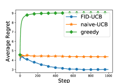
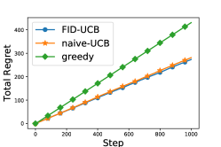
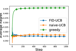
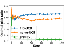
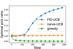
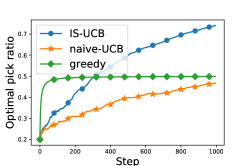
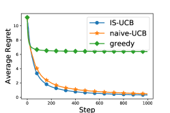
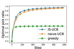
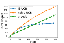
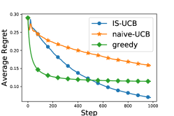
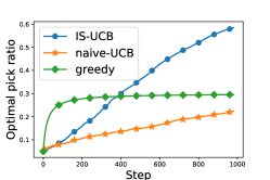
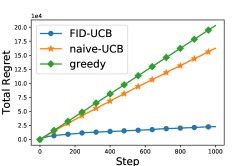
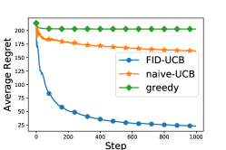
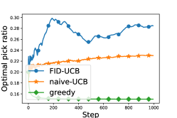
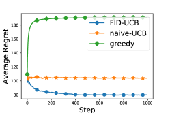
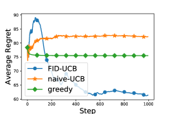
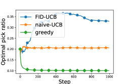
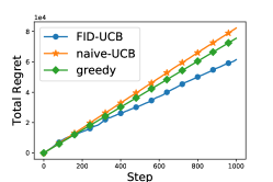
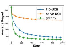
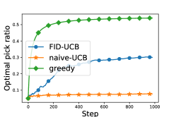
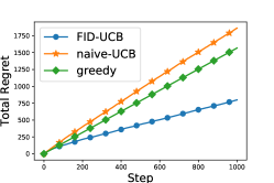
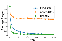
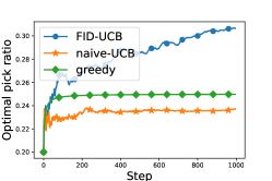
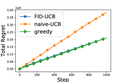
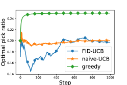
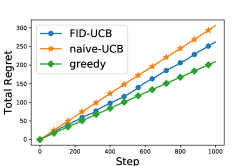
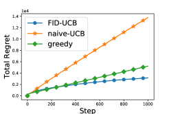
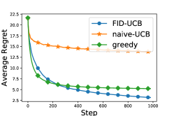
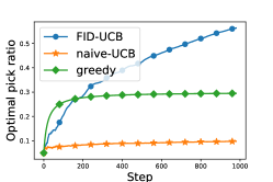
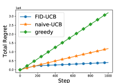
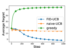
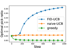
Experimental setup and performance metrics. We report three performance metrics at each step : 1) total regret, i.e., , 2) average regret, i.e., , and 3) optimal pick ratio, i.e., the ratio of picking the optimal model, which has the lowest empirical FID score or the highest empirical IS score for 50k generated images. For all the experiments, we use a batch size of 5, and the total evaluation step is . Hence the total generated samples for each trial is k. Results are averaged over 20 trials. Due to the limited space, we postpone parts of the results to Appendix C.
7.1 Empirical Results of Online FID-based Evaluation
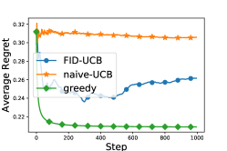
Performance on pretrained generators under different embeddings. The results are summarized in Figure 1, where each row and each column correspond to one dataset and one performance metric, respectively. The results show that FID-UCB (blue) outperforms naive-UCB (orange) and the greedy algorithm (green). We observe that naive-UCB fails to distinguish between different generators and makes uniform selections on the CIFAR10 and the ImageNet datasets, while FID-UCB recognizes the optimal one. This shows that the generator-dependent optimistic FID (6) can better exploit the properties of the generator, which is key to the sample-efficient online evaluation. On the FFHQ dataset, all the generators attain very similar FID scores (the largest gap is less than 0.7), which may explain why FID-UCB has a similar performance to naive-UCB. We reran these experiments using DINOv2-ViT-L/14-based [33] and CLIP-based [7] embeddings. (The results are summarized in Figures 5 and 6 in Appendix C, respective.) The numerical results show that FID-UCB can maintain satisfactory performance over different embeddings.
CIFAR10 (G=5)
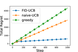
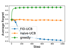
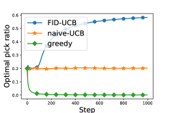

ImageNet (G=5)
FFHQ (G=5) \stackunderTotal regret \stackunderAverage regret \stackunderOptimal pick ratio
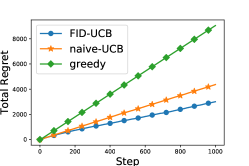
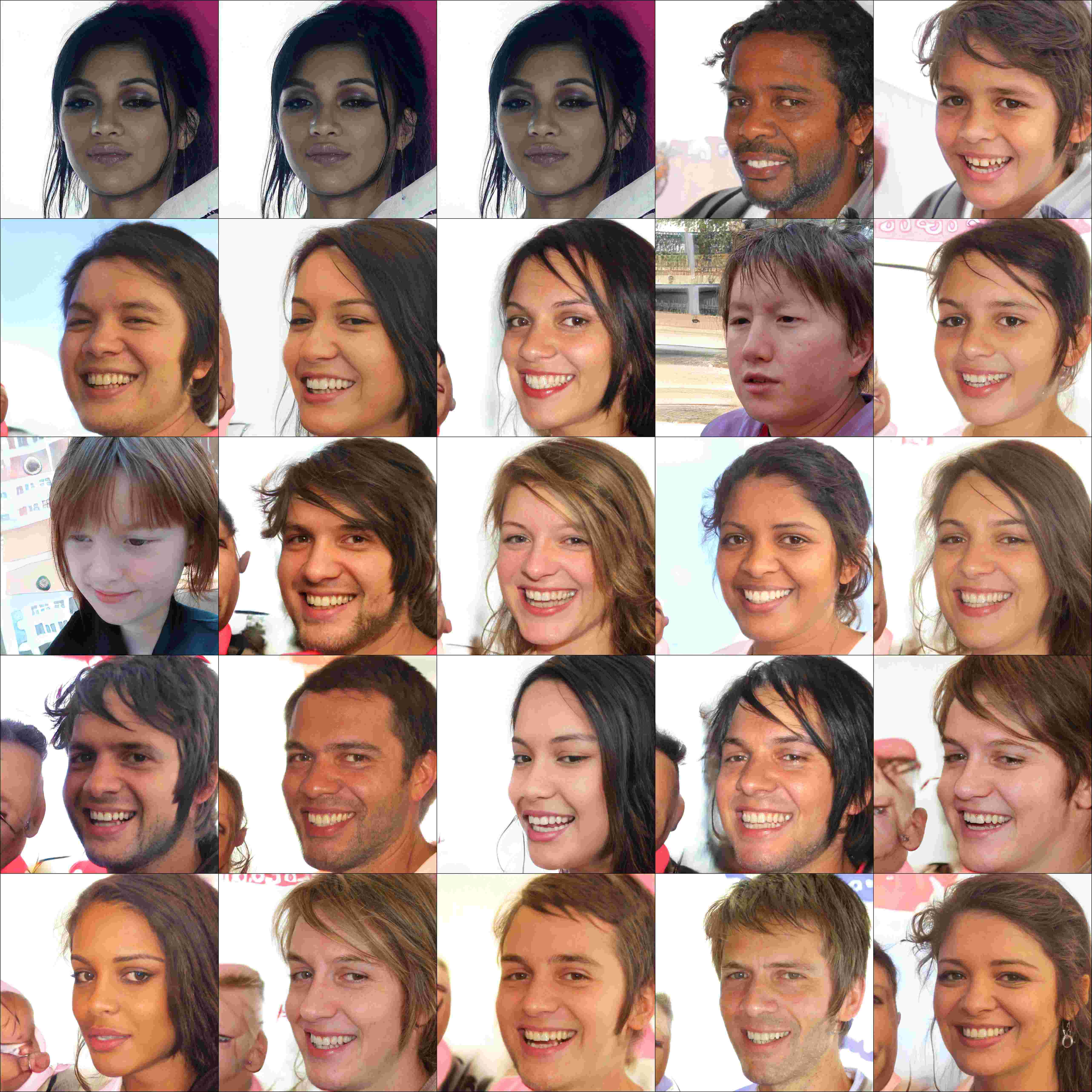
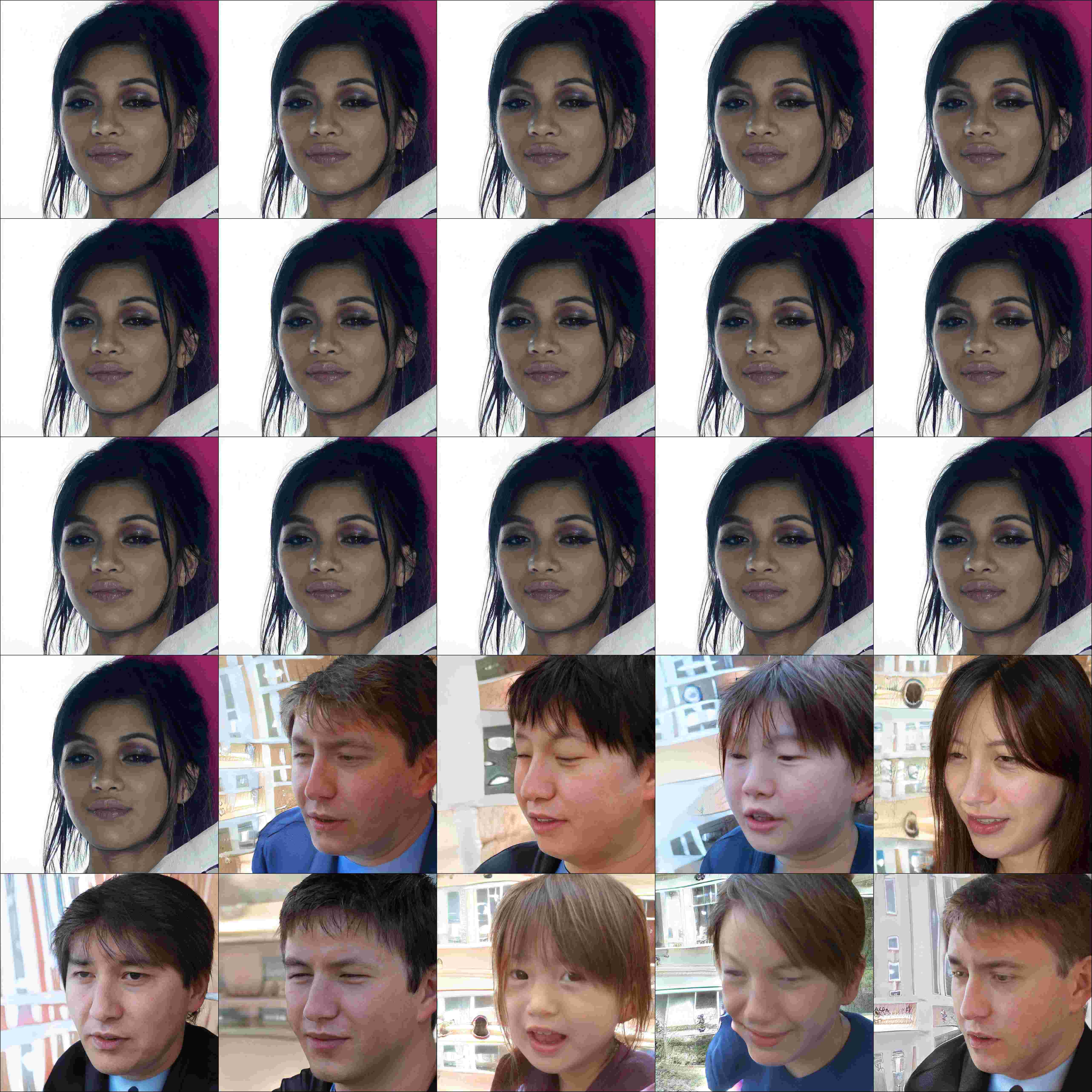
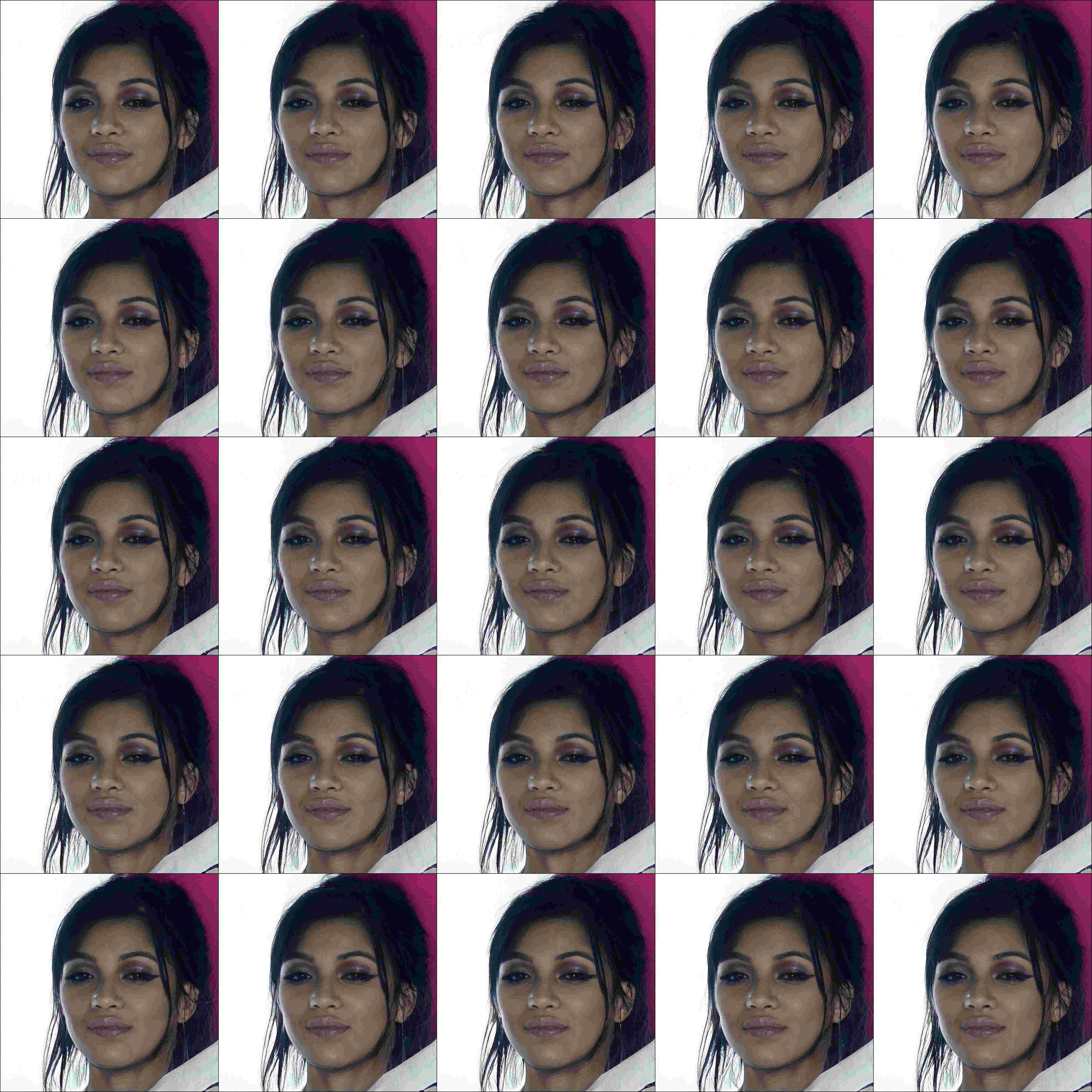
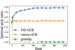
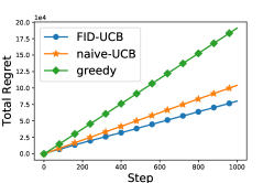
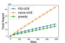
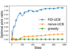
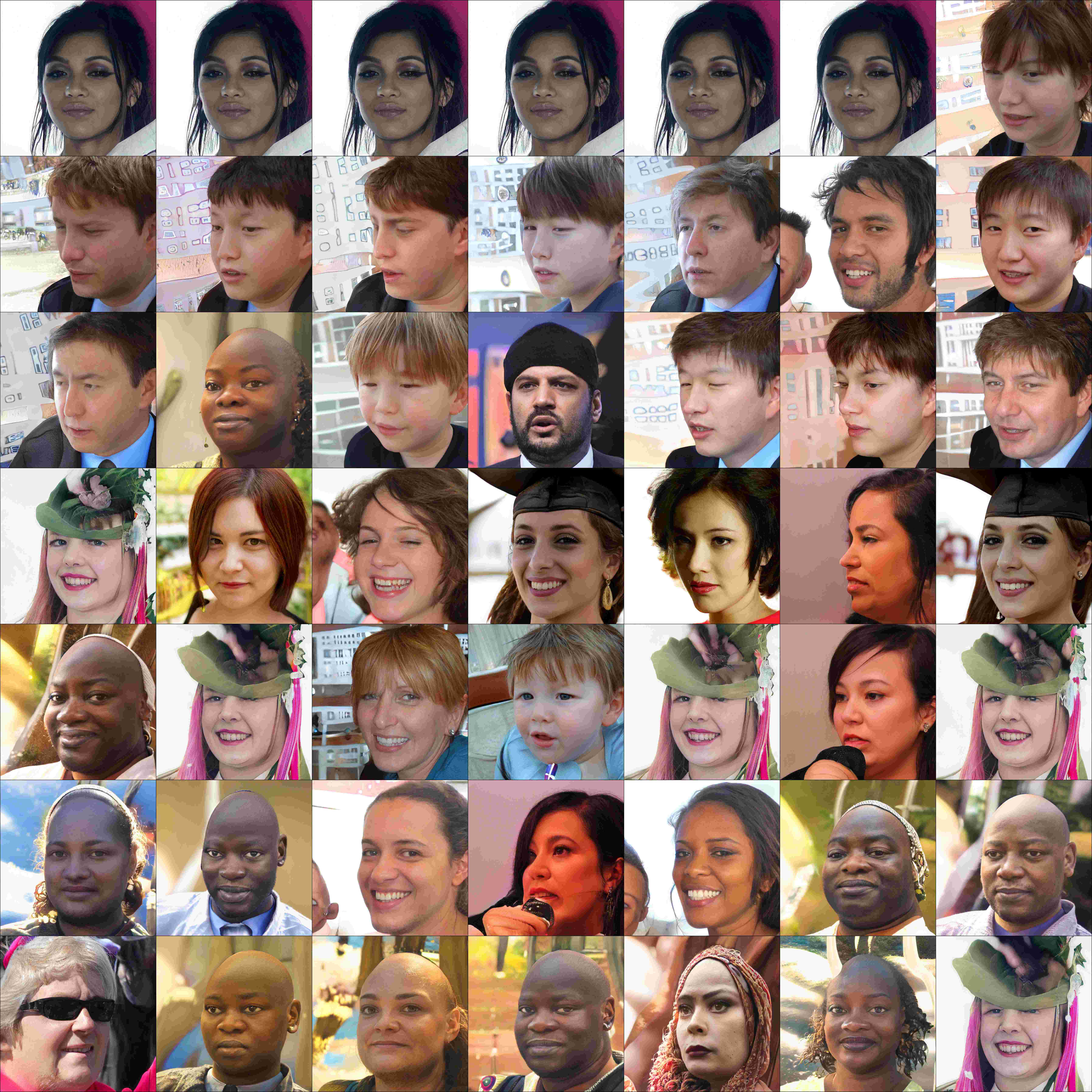
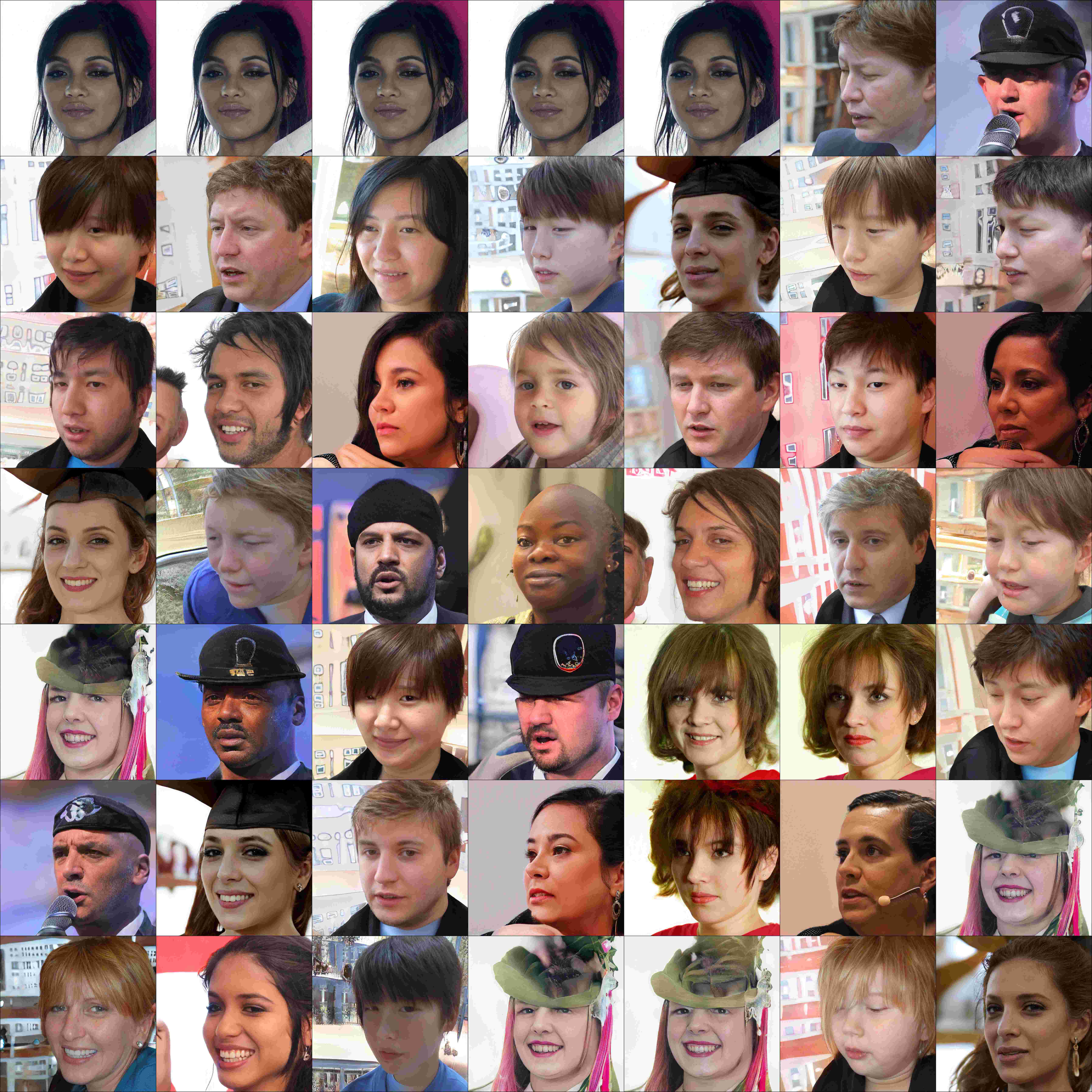
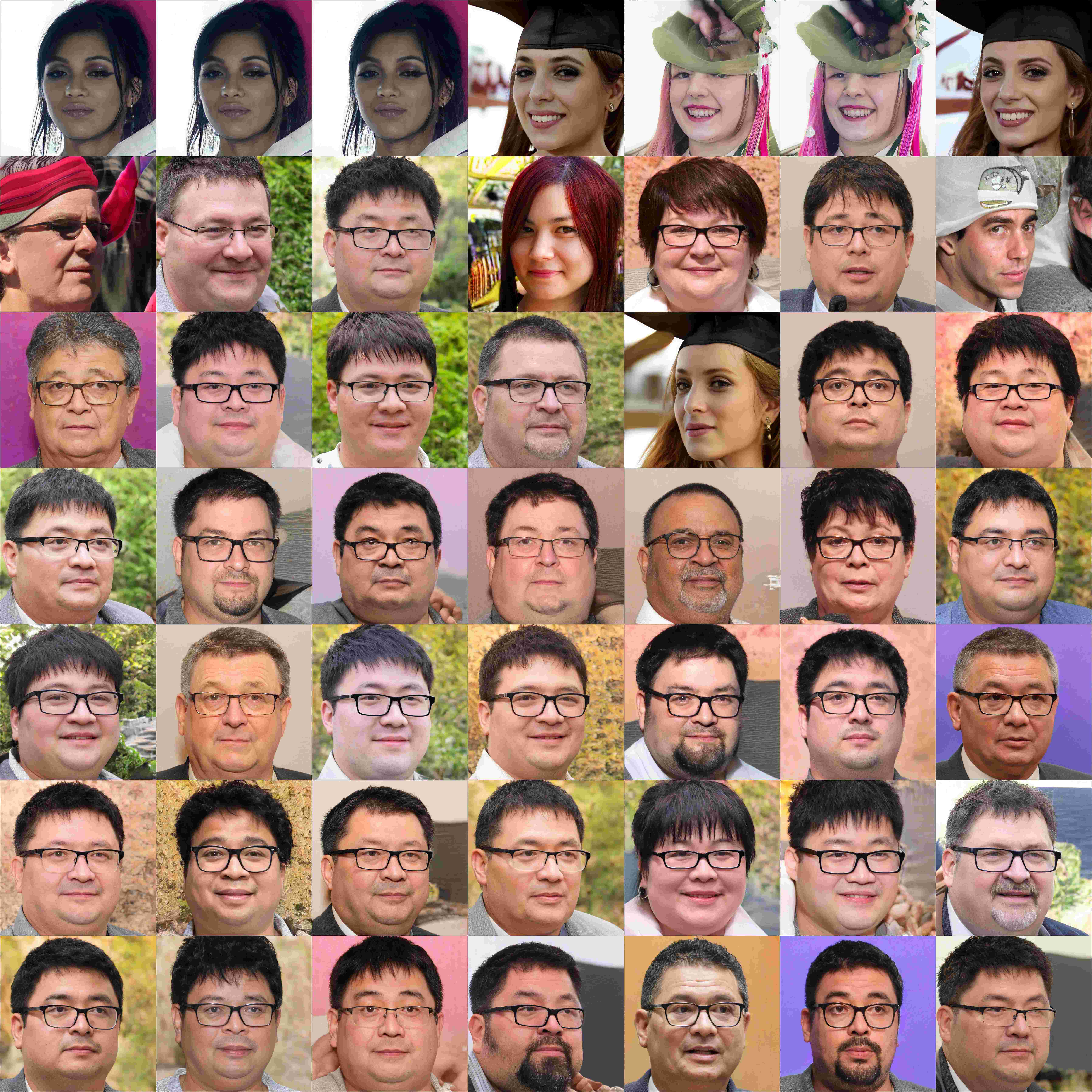
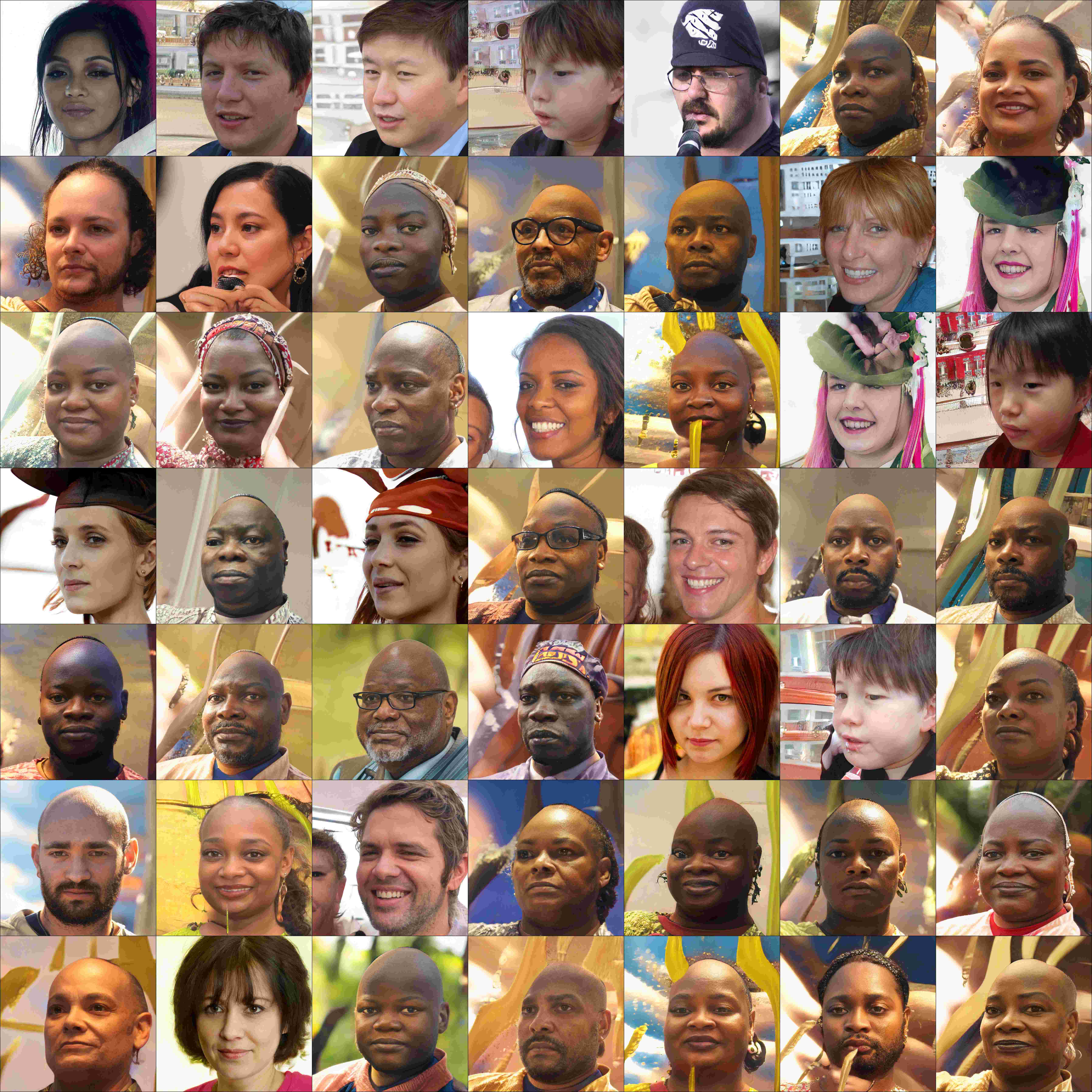
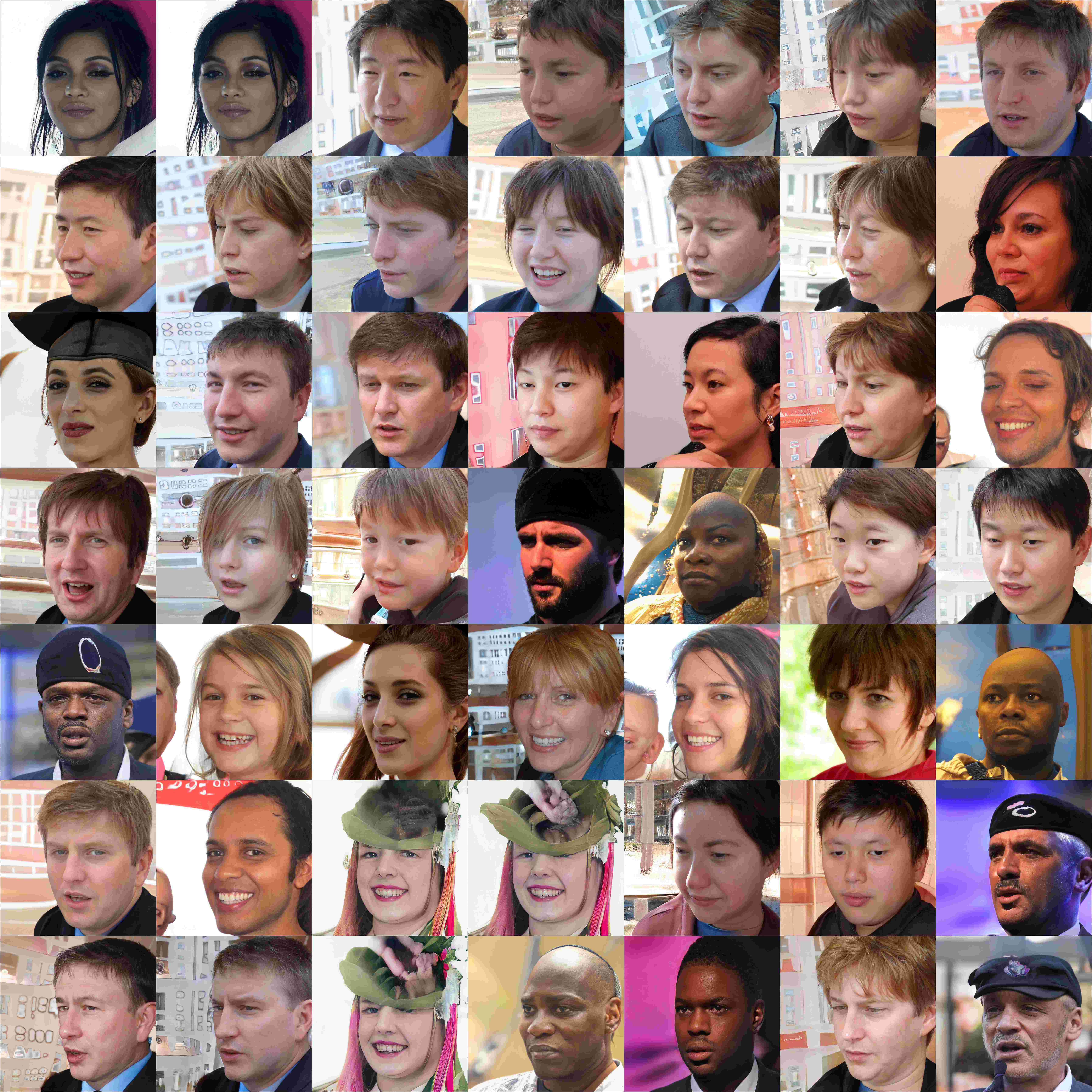
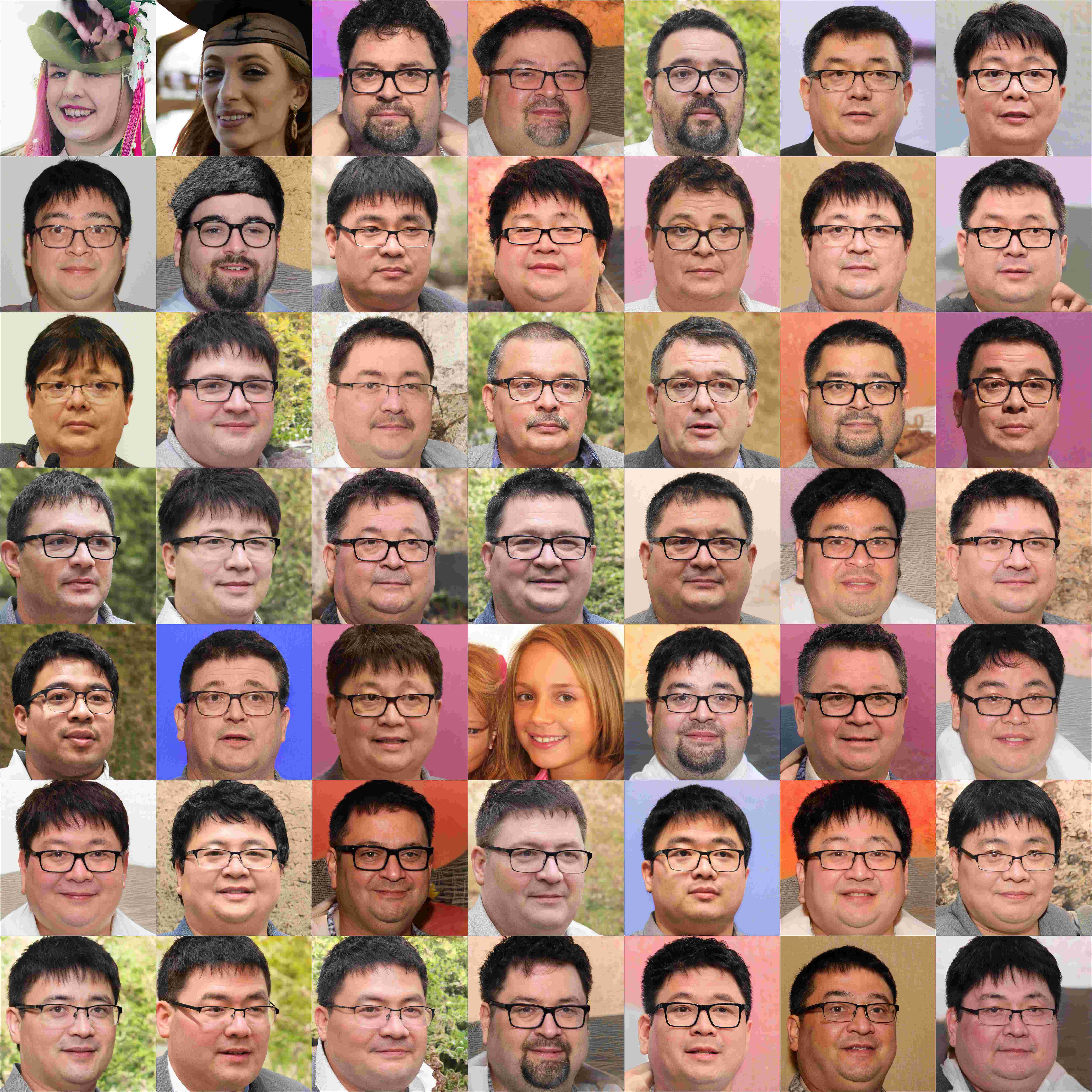
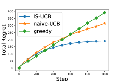
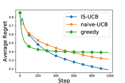
Performance on variance-controlled generators. We summarize the results in Figure 2. FID-UCB (blue) significantly outperforms naive-UCB and the greedy algorithm. The results for DINOv2-based and CLIP-based FID are provided in Figures 5 and 6 in Appendix C. We ran the evaluation on AFHQ Dog dataset, and the results are presented in Figure 7 in the Appendix. Furthermore, we display the generated images to visualize the quality and diversity of the samples queried by different algorithms. The results suggest that FID-UCB consistently queries images that are diverse and of high quality. In contrast, naive-UCB kept querying a proportion of images from the collapsed generator (the one with the smallest truncation parameter), and the greedy algorithm even stuck to it.
FFHQ (G=20)
![[Uncaptioned image]](/html/2406.07451/assets/x10.png)
![[Uncaptioned image]](/html/2406.07451/assets/x11.png)
Step 500
Step 1000 \stackunderFID-UCB \stackunderNaive UCB \stackunderGreedy
![[Uncaptioned image]](/html/2406.07451/assets/results/summary_1000_UCB.jpg)
![[Uncaptioned image]](/html/2406.07451/assets/results/summary_1000_nUCB.jpg)
![[Uncaptioned image]](/html/2406.07451/assets/results/summary_1000_naive.jpg)
7.2 Results of Online IS-Based Evaluation
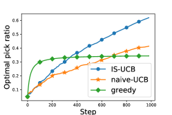
Performance on the pretrained generators. The results are summarized in Figure 3. IS-UCB (blue) attains significantly better performance than naive-UCB (orange) and the greedy algorithm (green) on CIFAR10 and FFHQ datasets.
CIFAR10 (G=5)
![[Uncaptioned image]](/html/2406.07451/assets/x13.png)
![[Uncaptioned image]](/html/2406.07451/assets/x14.png)
ImageNet (G=5)
![[Uncaptioned image]](/html/2406.07451/assets/x18.png)
FFHQ (G=5) \stackunderTotal regret \stackunderAverage regret \stackunderOptimal pick ratio
![[Uncaptioned image]](/html/2406.07451/assets/x19.png)
![[Uncaptioned image]](/html/2406.07451/assets/x20.png)
![[Uncaptioned image]](/html/2406.07451/assets/x21.png)
Performance on variance-controlled generators. The results are summarized in Figure 4. Generated samples are plotted in Figure 8 in the Appendix. The results on the AFHQ Dog dataset are presented in Figure 9 in the Appendix.
FFHQ (G=20)
8 Conclusion
In this work, we studied an online learning problem aiming to identify the generative model with the best evaluation score among a set of models. We proposed the optimism-based FID-UCB and IS-UCB algorithms to address the online learning task and showed satisfactory numerical results for their application to image-based generative models. An interesting future direction to our work is to explore the application of other online learning frameworks, such as Thompson sampling, to address the online evaluation problem. Also, while we mostly focused on standard image datasets for testing the proposed algorithms, the application of the proposed FID-UCB and IS-UCB to text-based and video-based generative models will be interesting for future studies. Such an application only requires applying text and video-based embeddings, as in Video IS [35], FVD [42], and FTD [19].
References
- Agrawal [1995] Rajeev Agrawal. Sample mean based index policies with o(log n) regret for the multi-armed bandit problem. Advances in Applied Probability, 27(4):1054–1078, 1995. ISSN 00018678. URL http://www.jstor.org/stable/1427934.
- Alaa et al. [2022] Ahmed Alaa, Boris Van Breugel, Evgeny S. Saveliev, and Mihaela van der Schaar. How faithful is your synthetic data? Sample-level metrics for evaluating and auditing generative models. In Kamalika Chaudhuri, Stefanie Jegelka, Le Song, Csaba Szepesvari, Gang Niu, and Sivan Sabato, editors, Proceedings of the 39th International Conference on Machine Learning, volume 162 of Proceedings of Machine Learning Research, pages 290–306. PMLR, 17–23 Jul 2022. URL https://proceedings.mlr.press/v162/alaa22a.html.
- Arjovsky et al. [2017] Martin Arjovsky, Soumith Chintala, and Léon Bottou. Wasserstein generative adversarial networks. In Doina Precup and Yee Whye Teh, editors, Proceedings of the 34th International Conference on Machine Learning, volume 70 of Proceedings of Machine Learning Research, pages 214–223. PMLR, 06–11 Aug 2017. URL https://proceedings.mlr.press/v70/arjovsky17a.html.
- Auer [2003] Peter Auer. Using confidence bounds for exploitation-exploration trade-offs. J. Mach. Learn. Res., 3(null):397–422, mar 2003. ISSN 1532-4435.
- Bińkowski et al. [2018] Mikołaj Bińkowski, Dougal J. Sutherland, Michael Arbel, and Arthur Gretton. Demystifying MMD GANs. In International Conference on Learning Representations, 2018. URL https://openreview.net/forum?id=r1lUOzWCW.
- Bubeck and Cesa-Bianchi [2012] Sébastien Bubeck and Nicolò Cesa-Bianchi. Regret analysis of stochastic and nonstochastic multi-armed bandit problems, 2012.
- Cherti et al. [2023] Mehdi Cherti, Romain Beaumont, Ross Wightman, Mitchell Wortsman, Gabriel Ilharco, Cade Gordon, Christoph Schuhmann, Ludwig Schmidt, and Jenia Jitsev. Reproducible scaling laws for contrastive language-image learning. In Proceedings of the IEEE/CVF Conference on Computer Vision and Pattern Recognition, pages 2818–2829, 2023.
- Choi et al. [2020] Yunjey Choi, Youngjung Uh, Jaejun Yoo, and Jung-Woo Ha. Stargan v2: Diverse image synthesis for multiple domains. In Proceedings of the IEEE/CVF Conference on Computer Vision and Pattern Recognition (CVPR), June 2020.
- Chong and Forsyth [2020] Min Jin Chong and David Forsyth. Effectively unbiased fid and inception score and where to find them, 2020.
- Daskalakis et al. [2018] Constantinos Daskalakis, Andrew Ilyas, Vasilis Syrgkanis, and Haoyang Zeng. Training GANs with optimism. In International Conference on Learning Representations, 2018. URL https://openreview.net/forum?id=SJJySbbAZ.
- Deng et al. [2009] J. Deng, W. Dong, R. Socher, L.-J. Li, K. Li, and L. Fei-Fei. ImageNet: A Large-Scale Hierarchical Image Database. In CVPR09, 2009.
- Dowson and Landau [1982] D.C Dowson and B.V Landau. The fréchet distance between multivariate normal distributions. Journal of Multivariate Analysis, 12(3):450–455, 1982. ISSN 0047-259X. doi: https://doi.org/10.1016/0047-259X(82)90077-X. URL https://www.sciencedirect.com/science/article/pii/0047259X8290077X.
- Friedman and Dieng [2023] Dan Friedman and Adji Bousso Dieng. The vendi score: A diversity evaluation metric for machine learning. Transactions on Machine Learning Research, 2023. ISSN 2835-8856. URL https://openreview.net/forum?id=g97OHbQyk1.
- Goodfellow et al. [2014] Ian Goodfellow, Jean Pouget-Abadie, Mehdi Mirza, Bing Xu, David Warde-Farley, Sherjil Ozair, Aaron Courville, and Yoshua Bengio. Generative adversarial nets. In Z. Ghahramani, M. Welling, C. Cortes, N. Lawrence, and K.Q. Weinberger, editors, Advances in Neural Information Processing Systems, volume 27. Curran Associates, Inc., 2014. URL https://proceedings.neurips.cc/paper_files/paper/2014/file/5ca3e9b122f61f8f06494c97b1afccf3-Paper.pdf.
- Grnarova et al. [2018] Paulina Grnarova, Kfir Y Levy, Aurelien Lucchi, Thomas Hofmann, and Andreas Krause. An online learning approach to generative adversarial networks. In International Conference on Learning Representations, 2018. URL https://openreview.net/forum?id=H1Yp-j1Cb.
- Han et al. [2023] Jiyeon Han, Hwanil Choi, Yunjey Choi, Junho Kim, Jung-Woo Ha, and Jaesik Choi. Rarity score : A new metric to evaluate the uncommonness of synthesized images. In The Eleventh International Conference on Learning Representations, 2023. URL https://openreview.net/forum?id=JTGimap_-F.
- Heusel et al. [2017] Martin Heusel, Hubert Ramsauer, Thomas Unterthiner, Bernhard Nessler, and Sepp Hochreiter. Gans trained by a two time-scale update rule converge to a local nash equilibrium. In I. Guyon, U. Von Luxburg, S. Bengio, H. Wallach, R. Fergus, S. Vishwanathan, and R. Garnett, editors, Advances in Neural Information Processing Systems, volume 30. Curran Associates, Inc., 2017. URL https://proceedings.neurips.cc/paper_files/paper/2017/file/8a1d694707eb0fefe65871369074926d-Paper.pdf.
- Hoeffding [1963] Wassily Hoeffding. Probability inequalities for sums of bounded random variables. Journal of the American Statistical Association, 58(301):13–30, 1963. ISSN 01621459. URL http://www.jstor.org/stable/2282952.
- Iyer and Hou [2023] Srikrishna Iyer and Teng Teck Hou. Gat-gan : A graph-attention-based time-series generative adversarial network, 2023.
- Jalali et al. [2023] Mohammad Jalali, Cheuk Ting Li, and Farzan Farnia. An information-theoretic evaluation of generative models in learning multi-modal distributions. In A. Oh, T. Naumann, A. Globerson, K. Saenko, M. Hardt, and S. Levine, editors, Advances in Neural Information Processing Systems, volume 36, pages 9931–9943. Curran Associates, Inc., 2023. URL https://proceedings.neurips.cc/paper_files/paper/2023/file/1f5c5cd01b864d53cc5fa0a3472e152e-Paper-Conference.pdf.
- Jiralerspong et al. [2023] Marco Jiralerspong, Joey Bose, Ian Gemp, Chongli Qin, Yoram Bachrach, and Gauthier Gidel. Feature likelihood score: Evaluating the generalization of generative models using samples. In Thirty-seventh Conference on Neural Information Processing Systems, 2023. URL https://openreview.net/forum?id=l2VKZkolT7.
- Kang et al. [2023] MinGuk Kang, Joonghyuk Shin, and Jaesik Park. StudioGAN: A Taxonomy and Benchmark of GANs for Image Synthesis. IEEE Transactions on Pattern Analysis and Machine Intelligence (TPAMI), 2023.
- Karras et al. [2020] Tero Karras, Miika Aittala, Janne Hellsten, Samuli Laine, Jaakko Lehtinen, and Timo Aila. Training generative adversarial networks with limited data. In H. Larochelle, M. Ranzato, R. Hadsell, M.F. Balcan, and H. Lin, editors, Advances in Neural Information Processing Systems, volume 33, pages 12104–12114. Curran Associates, Inc., 2020. URL https://proceedings.neurips.cc/paper_files/paper/2020/file/8d30aa96e72440759f74bd2306c1fa3d-Paper.pdf.
- Kazemi and Sullivan [2014] Vahid Kazemi and Josephine Sullivan. One millisecond face alignment with an ensemble of regression trees. In 2014 IEEE Conference on Computer Vision and Pattern Recognition, pages 1867–1874, 2014. doi: 10.1109/CVPR.2014.241.
- Koltchinskii and Lounici [2017] Vladimir Koltchinskii and Karim Lounici. Concentration inequalities and moment bounds for sample covariance operators. Bernoulli, 23(1):110 – 133, 2017. doi: 10.3150/15-BEJ730. URL https://doi.org/10.3150/15-BEJ730.
- Krizhevsky et al. [2009] Alex Krizhevsky, Geoffrey Hinton, et al. Learning multiple layers of features from tiny images. 2009.
- Kynkäänniemi et al. [2019] Tuomas Kynkäänniemi, Tero Karras, Samuli Laine, Jaakko Lehtinen, and Timo Aila. Improved precision and recall metric for assessing generative models. In H. Wallach, H. Larochelle, A. Beygelzimer, F. d'Alché-Buc, E. Fox, and R. Garnett, editors, Advances in Neural Information Processing Systems, volume 32. Curran Associates, Inc., 2019. URL https://proceedings.neurips.cc/paper_files/paper/2019/file/0234c510bc6d908b28c70ff313743079-Paper.pdf.
- Kynkäänniemi et al. [2023] Tuomas Kynkäänniemi, Tero Karras, Miika Aittala, Timo Aila, and Jaakko Lehtinen. The role of imagenet classes in fréchet inception distance. In The Eleventh International Conference on Learning Representations, 2023. URL https://openreview.net/forum?id=4oXTQ6m_ws8.
- Lai and Robbins [1985] T.L Lai and Herbert Robbins. Asymptotically efficient adaptive allocation rules. Advances in Applied Mathematics, 6(1):4–22, 1985. ISSN 0196-8858. doi: https://doi.org/10.1016/0196-8858(85)90002-8. URL https://www.sciencedirect.com/science/article/pii/0196885885900028.
- Lounici [2014] Karim Lounici. High-dimensional covariance matrix estimation with missing observations. Bernoulli, 20(3):1029–1058, 2014. ISSN 13507265. URL http://www.jstor.org/stable/42919424.
- Maurer and Pontil [2009] Andreas Maurer and Massimiliano Pontil. Empirical bernstein bounds and sample variance penalization, 2009.
- Naeem et al. [2020] Muhammad Ferjad Naeem, Seong Joon Oh, Youngjung Uh, Yunjey Choi, and Jaejun Yoo. Reliable fidelity and diversity metrics for generative models. In Hal Daumé III and Aarti Singh, editors, Proceedings of the 37th International Conference on Machine Learning, volume 119 of Proceedings of Machine Learning Research, pages 7176–7185. PMLR, 13–18 Jul 2020. URL https://proceedings.mlr.press/v119/naeem20a.html.
- Oquab et al. [2024] Maxime Oquab, Timothée Darcet, Théo Moutakanni, Huy Vo, Marc Szafraniec, Vasil Khalidov, Pierre Fernandez, Daniel Haziza, Francisco Massa, Alaaeldin El-Nouby, Mahmoud Assran, Nicolas Ballas, Wojciech Galuba, Russell Howes, Po-Yao Huang, Shang-Wen Li, Ishan Misra, Michael Rabbat, Vasu Sharma, Gabriel Synnaeve, Hu Xu, Hervé Jegou, Julien Mairal, Patrick Labatut, Armand Joulin, and Piotr Bojanowski. Dinov2: Learning robust visual features without supervision, 2024.
- Park et al. [2024] Chanwoo Park, Xiangyu Liu, Asuman Ozdaglar, and Kaiqing Zhang. Do llm agents have regret? a case study in online learning and games, 2024.
- Saito et al. [2020] Masaki Saito, Shunta Saito, Masanori Koyama, and Sosuke Kobayashi. Train sparsely, generate densely: Memory-efficient unsupervised training of high-resolution temporal gan. International Journal of Computer Vision, 128(10–11):2586–2606, May 2020. ISSN 1573-1405. doi: 10.1007/s11263-020-01333-y. URL http://dx.doi.org/10.1007/s11263-020-01333-y.
- Sajjadi et al. [2018] Mehdi S. M. Sajjadi, Olivier Bachem, Mario Lucic, Olivier Bousquet, and Sylvain Gelly. Assessing generative models via precision and recall. In S. Bengio, H. Wallach, H. Larochelle, K. Grauman, N. Cesa-Bianchi, and R. Garnett, editors, Advances in Neural Information Processing Systems, volume 31. Curran Associates, Inc., 2018. URL https://proceedings.neurips.cc/paper_files/paper/2018/file/f7696a9b362ac5a51c3dc8f098b73923-Paper.pdf.
- Salimans et al. [2016] Tim Salimans, Ian Goodfellow, Wojciech Zaremba, Vicki Cheung, Alec Radford, Xi Chen, and Xi Chen. Improved techniques for training gans. In D. Lee, M. Sugiyama, U. Luxburg, I. Guyon, and R. Garnett, editors, Advances in Neural Information Processing Systems, volume 29. Curran Associates, Inc., 2016. URL https://proceedings.neurips.cc/paper_files/paper/2016/file/8a3363abe792db2d8761d6403605aeb7-Paper.pdf.
- Sani et al. [2012] Amir Sani, Alessandro Lazaric, and Rémi Munos. Risk-aversion in multi-armed bandits. In F. Pereira, C.J. Burges, L. Bottou, and K.Q. Weinberger, editors, Advances in Neural Information Processing Systems, volume 25. Curran Associates, Inc., 2012. URL https://proceedings.neurips.cc/paper_files/paper/2012/file/83f2550373f2f19492aa30fbd5b57512-Paper.pdf.
- Stein et al. [2023] George Stein, Jesse Cresswell, Rasa Hosseinzadeh, Yi Sui, Brendan Ross, Valentin Villecroze, Zhaoyan Liu, Anthony L Caterini, Eric Taylor, and Gabriel Loaiza-Ganem. Exposing flaws of generative model evaluation metrics and their unfair treatment of diffusion models. In A. Oh, T. Naumann, A. Globerson, K. Saenko, M. Hardt, and S. Levine, editors, Advances in Neural Information Processing Systems, volume 36, pages 3732–3784. Curran Associates, Inc., 2023. URL https://proceedings.neurips.cc/paper_files/paper/2023/file/0bc795afae289ed465a65a3b4b1f4eb7-Paper-Conference.pdf.
- Szegedy et al. [2016] Christian Szegedy, Vincent Vanhoucke, Sergey Ioffe, Jon Shlens, and Zbigniew Wojna. Rethinking the inception architecture for computer vision. In 2016 IEEE Conference on Computer Vision and Pattern Recognition (CVPR), pages 2818–2826, 2016. doi: 10.1109/CVPR.2016.308.
- Thompson [1933] William R. Thompson. On the likelihood that one unknown probability exceeds another in view of the evidence of two samples. Biometrika, 25(3/4):285–294, 1933. ISSN 00063444. URL http://www.jstor.org/stable/2332286.
- Unterthiner et al. [2019] Thomas Unterthiner, Sjoerd van Steenkiste, Karol Kurach, Raphaël Marinier, Marcin Michalski, and Sylvain Gelly. FVD: A new metric for video generation, 2019. URL https://openreview.net/forum?id=rylgEULtdN.
- Wainwright [2019] Martin J. Wainwright. High-Dimensional Statistics: A Non-Asymptotic Viewpoint. Cambridge Series in Statistical and Probabilistic Mathematics. Cambridge University Press, 2019.
- Weinberger and Yemini [2023] Nir Weinberger and Michal Yemini. Multi-armed bandits with self-information rewards. IEEE Transactions on Information Theory, 69(11):7160–7184, 2023. doi: 10.1109/TIT.2023.3299460.
- Zhang et al. [2024] Jingwei Zhang, Cheuk Ting Li, and Farzan Farnia. An interpretable evaluation of entropy-based novelty of generative models. In International Conference on Machine Learning (ICML 2024), 2024.
- Zhivotovskiy [2022] Nikita Zhivotovskiy. Dimension-free bounds for sums of independent matrices and simple tensors via the variational principle, 2022.
- Zhu and Tan [2020] Qiuyu Zhu and Vincent Tan. Thompson sampling algorithms for mean-variance bandits. In Hal Daumé III and Aarti Singh, editors, Proceedings of the 37th International Conference on Machine Learning, volume 119 of Proceedings of Machine Learning Research, pages 11599–11608. PMLR, 13–18 Jul 2020. URL https://proceedings.mlr.press/v119/zhu20d.html.
Appendix A Proofs in Section 5: FID Evaluation
A.1 Proof of Theorem 5.1: Optimistic FID Score
Proof.
The proof of Theorem 5.1 is based on Theorem A.1 and Lemma A.2 in the Appendix. Specifically, Inequality (16) in Theorem A.1 in Appendix A.3 decomposes the estimation error of the empirical FID score (4) into the errors in estimating the mean (i.e., ) and the covariance matrix (i.e., ). Next, Lemma A.2 in Appendix A.4 derives generator-dependent concentration errors for the mean and the covariance matrix. Combining ∎
A.2 Proof of Theorem 5.2: Regret of FID-UCB
Proof.
Recall that denotes the generator picked at the -th step. For convenience, we denote by the optimistic FID of generator computed at step . We denote by the number of images generated by model after steps. First, by Theorem A.2 and a union bound over steps, with probability at least , we have that for any step and . Hence, we have that
By the definition of , we further derive that
where is the bonus function given by Equation (7). Therefore, the regret is further bounded by
where logarithmic factors are hidden in the notation . Here, we use the fact that
where is the batch size, and is the number of images generated by model at the last step . ∎
A.3 Concentration of Empirical FID (4)
Theorem A.1 (Concentration of empirical FID (4)).
Assume the covariance matrix is positive strictly definite, and we denote by its eigendecomposition. Then, with probability at least , we have that
| (16) | ||||
Proof.
Recall that for any generator , we have that
(1) Bound . Note that
We derive
| (17) | ||||
(2) Bound . By Theorem A.3 in Appendix A.5, if the covariance matrix is positive strictly definite, then it holds that
| (18) |
(3) Bound . Note that
| (19) |
Next, we bound the two terms in the last inequality. Let . For the first term, we have that
where we denote by the eigendecomposition of . Note that the random vector has distribution . We have that
where ’s are the eigenvalues of , are independent standard normal, and hence ’s are independent Chi-square random variables. Therefore, we have that
| (20) |
where the last inequality holds with probability at least by Lemma E.5. In addition, for the second term, we derive that
| (21) |
A.4 Concentration of Mean Vector and Covariance Matrix
Lemma A.2 (Concentration of mean vector and covariance matrix).
Under the same conditions in Theorem A.1, with probability at least , we have that
| (22) |
and
| (23) |
where is the largest variance for the elements in , and is the effective rank of .
Proof.
1. Concentration of mean vector. Note that where has a multivariate distribution, which is the same as . We have that
where is the matrix norm. Let denote the mean vector. We further obtain that
| (24) |
where and . For the first term, note that each diagonal element has the same distribution , where are i.i.d standard Gaussian. Then, with probability at least , we have that
| (25) |
where the first inequality holds by that is PSD, and the second inequality holds by Lemma E.10. For the second term,
where are i.i.d standard Gaussian. By Lemma E.11, with probability at least , it holds that
| (26) |
Combining Inequalities (25) and (26), we conclude that with probability at least , it holds that
| (27) |
2. Concentration of sample covariance matrix. we have that
| (28) |
where the last inequality holds by the triangle inequality of the L2 norm of the matrix. Note that the zero-mean random vector has a multivariate distribution (under the assumption of FID). For the first term, we evoke Lemma E.7. Then, with probability at least , it holds that
| (29) |
For the second term, we have that
which concludes the proof. ∎
A.5 Dimension-free Concentration of
Theorem A.3 (Dimension-free concentration of ).
Under the same conditions in Theorem A.1, we have that
| (30) |
Appendix B Proofs in Section 6: IS Evaluation
B.1 Proof of Theorem 6.1: Generator-Dependent Optimistic IS
B.2 Proof of Theorem 6.2: Regret of IS-UCB
Proof.
By Theorem 6.1 and union bound over steps, with probability at least , it holds that for all steps and , where is given by Equation (14). For convenience, we denote by the optimistic IS of generator computed at the -th step. Hence, we have that
where
Let be two disjoint set of steps such that . Specifically, contains steps where no element of the empirical marginal class distribution is clipped to , i.e., for all . Let denote the optimal Inception score. Hence, we have that
Recall for . For the first part, we further derive that
| (31) |
where , and is the upper bound of . For the second part, note that the number of steps where at least one element of is clipped to at most , where . Therefore, we have that
which concludes the proof. ∎
B.3 Optimistic marginal class distribution
Theorem B.1 (Optimistic marginal class distribution).
Let denote the empirical marginal class distribution. Let
where is the following element-wise operator
for any vectors . Then, we have that .
Proof.
Note that the function is concave and attains maximum at . It suffices to show that for all . If , then , which ensures that . In addition, if , then
The first case ensures that , and the second case ensures that . Both cases satisfy that . Therefore, we have that , which concludes the proof. ∎
B.4 Data-dependent optimistic marginal class distribution
Lemma B.2 (Optimistic marginal class distribution).
Let be generated images from generator . Define denote the error vector whose -th element is given by
where is the empirical variance for the -th class density. Then, with probability at least , we have that
satisfies that .
Proof.
It suffices that show that with probability at least . We evoke Theorem E.4 and conclude the proof. ∎
Appendix C Additional Experimental Results
C.1 Results of FID-Based Online Evaluation
1. Embeddings Extracted by DINOv2 [33].
We run FID-UCB, naive UCB, and the greedy algorithm where the feature of an image is extracted by DINOv2-ViT-L/14. The pretrained weights are downloaded from the official repository (licensed under Apache License 2.0).333https://github.com/facebookresearch/dinov2/tree/main The results are summarized in Figure 5.
CIFAR10 (G=5)
ImageNet (G=5)
FFHQ (G=5)
FFHQ (G=20) \stackunderTotal regret \stackunderAverage regret \stackunderOptimal pick ratio
2. Embeddings Extracted by CLIP [7].
We run FID-UCB, naive UCB, and the greedy algorithm where the feature of an image is extracted by CLIP. The pretrained weights are downloaded from the official repository.444https://github.com/mlfoundations/open_clip. Copyright (c) 2012-2021 Gabriel Ilharco, Mitchell Wortsman, Nicholas Carlini, Rohan Taori, Achal Dave, Vaishaal Shankar, John Miller, Hongseok Namkoong, Hannaneh Hajishirzi, Ali Farhadi, Ludwig Schmidt. The results are summarized in Figure 6. We note that in the FFHQ dataset, FID-UCB attains a low optimal pick ratio as the optimal generator and the second-best one attains almost the same CLIP-based FID.
CIFAR10 (G=5)

ImageNet (G=5)
FFHQ (G=5)
FFHQ (G=20) \stackunderTotal regret \stackunderAverage regret \stackunderOptimal pick ratio
3. Results on AFHQ Dog dataset.
The results are summarized in Figure 7.
AFHQ Dog (G=20)
C.2 Results of IS-Based Online Evaluation
1. Diversity and quality of the generated samples.
We examine the diversity and quality of the generated samples queried by IS-UCB, naive UCB, and the greedy algorithm (i.e., experiment in Figure 4). The results are summarized in Figure 8.
Step 500
Step 1000 \stackunderIS-UCB \stackunderNaive UCB \stackunderGreedy
2. Results on AFHQ Dog dataset.
The results are summarized in Figure 9.
AFHQ Dog (G=20)
Appendix D Additional Experimental details
1. Additional experiment setups.
All the experiments are run on a single Nvidia GeForce RTX 3090 GPU. For FID-based evaluation, each trial takes at most 2 hours to finish, depending on the dataset and the embedding pretrained model. For IS-based evaluation, each trial takes less than 30 minutes to finish.
2. List of pretrained generative models/generated image data.
For the CIFAR10 dataset, we compare pretrained models including SNGAN, ACGAN, BigGAN, ContraGAN, and BigGAN-CR. For the ImageNet dataset, we compare pretrained models including StyleGAN3, SNGAN, BigGAN, ContraGAN, and ReACGAN. The pretrained weights are downloaded from the StudioGAN repository [22]. For the FFHQ dataset, we compare StyleSwin, StyleNAT, StyleGAN2-ADA, StyleGAN-XL, and LDM, where we utilize the generated image datasets downloaded from the dgm-eval repository [39].
3. Implementation details of naive UCB for FID-based evaluation.
In FID-based evaluation, naive UCB upper bounds the error in estimating the mean vector by
which holds by the assumption of FID score that , with probability at least . In addition, the error in estimating the covariance matrix is bounded by
which follows from the exact same derivation in Inequality (28) and holds with probability at least (see Lemma E.6). Compared to the generator-dependent error bounds utilized by FID-UCB (i.e., Inequalities (27) and (29)), these bounds are dimension-dependent and do not fully exploit the properties of the generator. Finally, by the exact same analysis in the proof of Theorem 5.1, the following estimated FID
| (32) | ||||
lower bounds with probability at least .
4. Implementation details of naive UCB for IS-based evaluation.
In IS-based evaluation, naive UCB uses Hoeffding-type bonus terms. Specifically, the error vector in defining the optimistic marginal class distribution is given by , whose -th element is defined as
which ensures that with probability at least . In addition, the concentration error of is bounded by
which holds with probability at least . Therefore, the estimated IS is given by
| (33) |
By the exact same analysis in the proof of Theorem 6.1, it can be shown that with probability at least .
5. Additional implementation details of FID-UCB
To compute the bonus term (7), we need to estimate the following parameters: 1) : we set it to be a constant, e.g., 0.5; 2) : we estimate this term using the truncated covariance matrix with parameter , which is denoted by . The -th element of the truncated covariance matrix is if and is zero otherwise. In the experiments, we observe that a truncation parameter that is of the operator norm , i.e., , attains satisfying performance; 3) : we estimate this term by , where is the sample variance for the -th entry of the embedding . This avoids the computation for the eigendecomposition of the sample covariance matrix . The intuition is that when is diagonal, the operator norm coincides with the largest per-entry variance; 4) : while a direct approach is to estimate it by , we found that a better performance can be attained by using , where we utilize the fact that .
Appendix E Auxiliary Lemmas
Lemma E.1 (Concentration of Gaussian random variable).
Let . Then, it holds that
Equivalently, with probability at least , we have that
Lemma E.2 (Hoeffding’s inequality).
Let be i.i.d. random variables with values in and let . Then with probability at least in we have that
| (34) |
A drawback of Hoeffding’s inequality is that the confidence interval is distribution-agnostic, and always scales with order . For distribution with small variance, the following [18, Bennett’s inequality] provides a tighter concentration error.
Lemma E.3 (Bennett’s inequality).
Under the conditions of Theorem E.2, with probability at least in we have that
| (35) |
where is the variance .
When the exact variance is unknown, [31] provide a purely data-dependent bound with similar properties as Bennett’s inequality.
Lemma E.4 (Restatement of [31, Theorem 4]).
Under the conditions of Theorem E.2, we have that with probability at least in the i.i.d vector that
where is the sample variance.
Lemma E.5 (Concentration of Chi-square variables).
Let be i.i.d standard normal. Then, it holds that
Equivalently, with probability at least , we have that
Lemma E.6 (Restatement of [43, Example 6.3]).
Let be a random matrix from the -Gaussian ensemble, i.e., each row vector is drawn i.i.d. from a multivariate distribution. Then, with probability at least , we have that
| (36) |
where is the sample covariance matrix.
Lemma E.7 (Dimension-free concentration of sample covariance matrix [30, 25, 46]).
Let are i.i.d zero-mean and sub-Gaussian random vectors with parameter at most , whose covariance matrix is given by . Let
| (37) |
denote the effective rank. Then, with probability at least , the sample covariance matrix satisfies that
| (38) |
whenever .
Lemma E.8.
Let be positive semi-definite (PSD) matrices. Then, we have that
| (39) |
Proof.
Since and , by Courant-Fischer min-max theorem, it holds that and for their -th largest eigenvalues, which concludes the proof. ∎
Lemma E.9.
Let be positive semi-definite (PSD) matrices. Then, we have that
| (40) |
Proof.
First, we assume that both matrices and are positive strictly definite. Then,
where the last inequality holds by and (see Lemma E.12). For general PSD matrices and , note that
holds for any by our previous analysis. Since the trace map is continuous, ∎
Lemma E.10.
Let are i.i.d standard Gaussian. Then, with probability at least , it holds that
Proof.
Note that . By Lemma E.5, we have that
where is a chi-square random variable. Hence, with probability at least , it holds that
which concludes the proof. ∎
Lemma E.11.
Let be i.i.d standard Gaussian. Then, with probability at least , it holds that
Proof.
Note that .
where are i.i.d standard Gaussian. Observe that
where are i.i.d Chi-square distributed with 1 degree of freedom (since and are i.i.d standard Gaussian). Hence, by Lemma E.5 and a union bound, with probability at least ,
which concludes the proof. ∎
Lemma E.12.
Let denote two PSD matrices such that . Then, their inverse .
Proof.
It suffices to show that . Since shares the same eigenvalues with , which concludes the proof. ∎