Holographic and Gravity-Thermodynamic Approaches in Entropic Cosmology: Bayesian Assessment using late-time Data

Abstract

We investigate the cosmological implications of entropy-based approaches in the context of Holographic Dark Energy (HDE) and Gravity-Thermodynamics (GT) formalisms. We utilise the extended Barrow entropy form, with the index parameter $\Delta$, representing the fractal dimension of the horizon. We also test implementing different parameter ranges for $\Delta$, which can be extended to Tsallis’ interpretation within the same formal cosmology. We perform a Bayesian analysis to constrain the cosmological parameters using the Pantheon+, more recent DESy5, DESI, and, as a supplement, Quasar datasets. We find that the HDE model within almost all data combinations performs extremely well in comparison to the GT approach, which is usually strongly disfavored. Using the combination of DESy5+DESI alone, we find that the GT approaches are disfavored at $|\log\mathcal{B}|\sim 5.8$ and $|\log\mathcal{B}|\sim 6.2$ for the Barrow and Tsallis limits on $\Delta$, respectively, wrt $\Lambda$CDM model. While the HDE approach is statistically equivalent to $\Lambda$CDM when comparing the Bayesian evidence. We also investigate the evolution of the dark energy equation of state and place limits on the same, consistent with quintessence-like behaviour in the HDE approaches.

I Introduction

The discovery of the universe’s accelerated expansion through supernova (SNe) observations Riess et al. (1998) significantly transformed cosmological parameter estimation, necessitating the inclusion of the cosmological constant $\Lambda$. The $\Lambda$ Cold Dark Matter (${\Lambda\rm{CDM}}$) model emerged as the concordance cosmology after surviving numerous subsequent scrutinies using updated SNe datasets Betoule et al. (2014); Scolnic et al. (2018, 2022); Haridasu et al. (2018a); Abbott et al. (2024); Dam et al. (2017); Rubin and Hayden (2016) and successfully explained the Cosmic Microwave Background (CMB) Ade et al. (2016); Aghanim et al. (2020). Despite its success, ${\Lambda\rm{CDM}}$ presents significant challenges in achieving a physical understanding, especially given unresolved tensions in parameter estimates. The most notable of these is the $H_{0}$ tension, which has reached a significance level greater than $5\sigma$ Verde et al. (2019); Riess et al. (2022); Riess (2019). Various modifications to cosmological models have been proposed to address this tension Abdalla et al. (2022), as well as other milder tensions, such as the $S_{8}$ tension Riess (2019); Perivolaropoulos and Skara (2022); Efstathiou (2020); Freedman (2021); Verde et al. (2023).

This highlights the necessity to go beyond the standard model, with one promising avenue being the utilization of cosmological horizons. These are inspired by studies on black hole event horizons and their thermodynamic characteristics Wang et al. (2017a); del Campo et al. (2011); Saridakis et al. (2018); Nojiri et al. (2021), a concept known as the holographic approach based on the Holographic Principle Wang et al. (2017a); ’t Hooft (1993); Susskind (1995). It is now widely recognized that black hole systems exhibit behaviours reminiscent of thermodynamic systems Bekenstein (1994); Nappi and Pasquinucci (1992); Carlip (2014); Brown (1994); Oda (1994); Ghosh and Mitra (1996); Frolov (1995); Fursaev (1995); Louko and Whiting (1995); Liberati (1997); Solodukhin (1996); Carlip (1997); Frolov et al. (1996); Quevedo et al. (2024). This resemblance is encapsulated by the laws governing black hole thermodynamics, which include concepts such as the Bekenstein entropy and the Hawking temperature Bekenstein (1973, 1972); Hawking (1974, 1975).

The Bekenstein entropy, often termed “area entropy”, is directly proportional to the area of a black hole’s horizon and, thus, its radius squared Bekenstein (1973). The holographic approach draws an analogy between a black hole horizon and the apparent/future cosmological horizon Hsu (2004a); Oliveros et al. (2022); Bhardwaj et al. (2022); Astashenok and Tepliakov (2022, 2023); Tita et al. (2024) of the universe, suggesting that all the information contained within the universe is encoded on its horizon, akin to the event horizon of a black hole Saridakis et al. (2018); Salzano et al. (2017).

Another intriguing approach to understanding cosmic acceleration and possibly resolving tensions draws from gravity-thermodynamics formalism Saridakis (2020)Leon et al. (2021), which is once again based on the foundational concepts in black hole physics developed by Hawking and Bekenstein Bekenstein (1972, 1994). In this framework, we obtain the expansion history of the Universe implementing a thermodynamic perspectiveCai and Kim (2005), leveraging the relationship between entropy and horizon area, along with assumptions of local equilibrium conditions Asghari et al. (2024).

In order to build cosmological models from the above-mentioned approaches, we can use different non-extensive entropy formulations. The most common and standard of these is the Bekenstein-Hawking entropy Bekenstein (1972, 1994); Hawking (1975, 1976, 1974) given as,

$$S_{\rm BH}=\frac{A}{4G\hbar}$$ (1)

where A represents the area, $G,\,\hbar$ are the gravitational constant and reduced Planck constant, respectively.

We use non-extensive entropies as in systems with long-range interactions such as Newtonian gravity, the standard Gibbs-Boltzmann entropy cannot be used Tsallis and Cirto (2013) because, for such systems, the partition function diverges. Similarly, in the case of correlated systems such as strongly entangled particles and black holes (systems with entropy area law), the standard Gibbs extensive entropy does not apply. In these systems, the entropy is proportional to $L^{d-1}$ rather than $L^{d}$ (where $d$ represents the dimension of the system). Inspired by the generalizations of Gibbs-Bekenstein entropy, generalizations of Bekenstein-Hawking entropy were put forward mainly to make the black-hole entropy additive while still keeping it non-extensive. Examples of such generalized non-extensive entropies include Tsallis entropy Tsallis (1988), Rényi entropy Ré (1960), Barrow entropy Barrow (2020a), Sharma-Mittal entropy Sharma and Mittal (1975, 1977), and Kaniadakis entropy Kaniadakis (2005). See Nojiri et al. (2022) for a few generalised entropy forms and Ourabah (2024), where the entropy is derived starting with the gravitational potential. Applying these entropy formulations gives rise to various so-called ‘Entropic Cosmology’ models described and studied in Odintsov et al. (2023); Leon et al. (2021); Naeem and Bibi (2024); Saridakis et al. (2018); Nojiri et al. (2022); Nakarachinda et al. (2023); Fazlollahi (2023); Kord Zangeneh and Sheykhi (2023); Salehi (2023). However, our work primarily focuses on exploring Tsallis and Barrow entropies. Tsallis entropy was postulated to incorporate the concept of ‘multifractals’ by scaling the probability of occurrence of microstates by a factor, while Barrow entropy was conceptualized to account for the effects of ‘quantum gravity spacetime foam’ on the existing horizon structure Barrow (2020b). Although the physical principles underlying these two entropies are completely different, their formalisms are quite similar, with the only difference being the allowed ranges for a particular parameter (denoted as $\Delta$).

Contrasting the formal implications of entropic gravity through both the holographic principle (HP) ’t Hooft (1993); Srednicki (1993) implemented in Jacobson (2016) and gravity thermodynamics in Jacobson (1995); Padmanabhan (2005), Carroll and Remmen (2016) have earlier concluded that the former is more appropriate than the latter, which fails to provide a self-consistent definition for entropy. In this work, we essentially contrast the application of HP to the dark energy problem using the formalism described in Li (2004); Wang et al. (2017b), and gravity-thermodynamics formalism described in Jacobson (1995); Cai and Kim (2005); Padmanabhan (2005, 2010) and estimate the cosmological parameters by fitting the model against the cosmological observable that include recently published “Pantheon+”, “DESy5” supernovae Scolnic et al. (2022); Abbott et al. (2024), baryon acoustic oscillation “DESI” Adame et al. (2024) and quasar datasetRisaliti and Lusso (2019) through Bayesian analysis. We constrain cosmological parameters and validate their consistency against the standard ${\Lambda\rm{CDM}}$ model. We further estimate the Bayesian evidence to determine which of the models is favoured by the data as it is our primary objective to test which of the following approaches, namely Holographic or Gravity-Thermodynamics, is in better agreement with the data and how these two approaches fare against the $\Lambda$CDM. As a supplementary analysis, we also assess the dark energy equation of the state and its dynamical behaviour within these extended models.

The paper is structured as follows: Section II delves into the cosmological modelling, Section II.1 and Section II.2 address the Barrow Holographic Dark Energy and Barrow gravity-thermodynamics approaches, respectively. The observational dataset is presented in Section III, followed by our methodology and results in Section IV, and conclusions in Section V. Unless otherwise mentioned, we write all expressions in natural units $k_{\rm B}=c=\hbar=1$.

II Modelling

In this section, we briefly describe the two entropy-based approaches, namely the Holographic and gravity-thermodynamics approaches. For this, we utilize the Barrow entropy formalism Barrow (2020a), which is mathematically equivalent to the Tsallis entropy formalismTsallis and Cirto (2013) as both formalisms share the same parametric form, however, they allow for varied parameter spaces and have different physical interpretations.

The Barrow entropy proposal for the black hole surface area is based on introducing a fractal structure for the horizon geometry. This model consists of a three-dimensional spherical analogue of a ’Koch Snowflake’, employing an infinite diminishing hierarchy of touching spheres around the Schwarzschild event horizon. Through this method, a fractal structure for the horizon is created with finite volume and infinite area Barrow (2020c); Denkiewicz et al. (2023); Nojiri et al. (2022). Consequently, this model predicts an entropy different from Bekenstein-Hawking, where the entropy is formalized as

$$S_{\rm B}=\left(\frac{A}{A_{\rm P}}\right)^{1+\frac{\Delta}{2}}$$ (2)

Here, $A$ is the horizon area, $A_{\rm P}$ is the Planck area, and $\Delta$ is the free parameter representing the fractal dimension, bounded by $0\leq\Delta\leq 1$. We keep the introduction to the modelling brief as it has been studied and discussed extensively Odintsov et al. (2023); Leon et al. (2021); Naeem and Bibi (2024); Saridakis et al. (2018); Nojiri et al. (2022); Nakarachinda et al. (2023); Fazlollahi (2023); Kord Zangeneh and Sheykhi (2023); Salehi (2023).

II.1 Holographic dark energy

According to the Holographic Principle, the dark energy density of the Universe is given by $\rho_{\rm HDE}=\mathcal{S}_{\text{eff}}L^{-4}$ Wang et al. (2017b); Li (2004), where $\mathcal{S}_{\text{eff}}$ is the effective entropy and $L$ is the cosmological length scale, which can be interpreted as either the Hubble horizon, particle horizon, or future horizon. The dark energy density for the Barrow HDE model (using eq. 2), can be expressed as

$$\rho_{\rm HDE}=BL^{\Delta-2},$$ (3)

where $B$ is a free parameter with dimensions $[L]^{-(\Delta+2)}$. In the limiting case, where $\Delta=0$, this formalism reduces to the standard Holographic Dark Energy (HDE) Wang et al. (2017b); Li (2004),

$$\rho_{\rm HDE}=3C^{2}{M_{\rm P}}^{2}L^{-2},\qquad B=3C^{2}{M_{\rm P}}^{2}.$$ (4)

While the choice of the cosmological length scale is still an open issue, it has been argued in(Hsu, 2004b) that Hubble horizon ($H^{-1}$) cannot be used in the Holographic Dark energy case as it gives rise to inconsistencies, see also Davis and Lineweaver (2004); Dabrowski and Salzano (2020). Following the approaches used inLi (2004); Denkiewicz et al. (2023); Salzano et al. (2017) we utilise the future horizon as the cosmological length scale, which is given as,

$$R_{\rm h}=a\int_{t}^{\infty}\frac{{\rm d}t}{a}\equiv a\int_{a}^{\infty}\frac{{\rm d}a}{Ha^{2}}$$ (5)

Consequently, the dark energy density $\rho_{\rm HDE}$ can now be written as

$$\rho_{\rm HDE}=BR_{\rm h}^{\Delta-2}.$$ (6)

The Friedmann and Raychaudhuri equations in a flat universe with dark energy($\rho_{\rm HDE}$), matter($\rho_{\rm m}$) and radiation($\rho_{\rm\gamma}$) are,

$$H^{2} = \frac{1}{3{M_{\rm P}}^{2}}\left(\rho_{\rm m}+\rho_{\rm HDE}+\rho_{\rm\gamma}\right)$$ (7)

$$-\dot{H} = \frac{1}{2{M_{\rm P}}^{2}}\left(\rho_{\rm m}+\rho_{\rm HDE}+P_{\rm DE}+\rho_{\rm\gamma}+P_{\rm\gamma}\right)$$ (8)

where $P_{\rm I=\{HDE,\gamma\}}$ are the pressure terms for dark energy and radiation, respectively. We have already assumed pressureless matter ($P_{\rm m}=0$). The radiation pressure and energy density are related as $P_{r}=\frac{\rho_{r}}{3}$. One can now introduce the convenient fractional energy density parameters as $\Omega_{\rm i}=\frac{\rho_{\rm i}}{3{M_{\rm P}}^{2}H^{2}}$, where $\rm{i\in\{m,HDE,\gamma\}}$ can be substituted for matter, dark energy and radiation components, respectively. Substituting $\rho_{\rm HDE}$ from eq. 6 for the fractional energy density and using the future horizon definition in eq. 5 yields,

$$a\int_{a}^{\infty}\frac{{\rm d}a}{Ha^{2}}=\left(\frac{3{M_{\rm P}}^{2}H^{2}\Omega_{\rm HDE}}{B}\right)^{\frac{1}{\Delta-2}}$$ (9)

Finally, $\rho_{\rm m}$ = ${\rho_{\rm m0}}/{a^{3}}$ and $\rho_{\rm\gamma}$ = ${\rho_{\rm{\gamma 0}}}/{a^{4}}$, with $\rho_{\rm m0}$ and $\rho_{\rm\gamma 0}$ as the value of the matter and radiation-energy density at the present epoch $(a=1)$. Therefore, $\Omega_{\rm m}=\Omega_{\rm m0}H_{0}^{2}/{a^{3}H^{2}}$ and $\Omega_{\rm\gamma}=\Omega_{\rm\gamma 0}H_{0}^{2}/{a^{4}H^{2}}$, where the closure condition ensures $\Omega_{\rm m0}+\Omega_{\rm HDE}(a=1)+\Omega_{\rm\gamma 0}=1$. Using the definitions of $\Omega_{\rm m}$, $\Omega_{\rm\gamma}$ as mentioned above and the closure condition, we can write the expansion rate as,

$$H(a)=H_{0}\sqrt{\frac{\Omega_{\rm m0}a^{-3}+\Omega_{\rm\gamma 0}a^{-4}}{1-\Omega_{\rm HDE}(a)}}$$ (10)

Utilising eq. 10 in eq. 9 and differentiating both sides w.r.t $a$ gives the evolution of $\Omega_{\rm HDE}$ as,

$$\begin{split}\frac{\Omega_{\rm HDE}^{\prime}(a)}{[1-\Omega_{\rm HDE}(a)]}&=\frac{\left(2+{\Delta}\right)\Omega_{\rm\gamma 0}a^{-4}+(1+\Delta)\Omega_{\rm m0}a^{-3}}{\Omega_{\rm m0}a^{-3}+\Omega_{\rm\gamma 0}a^{-4}}+\\ &\left[1-\Omega_{\rm HDE}(a)\right]^{\frac{\Delta/2}{\Delta-2}}\Omega_{\rm HDE}(a)^{\frac{1}{2-\Delta}}Q(a)\end{split}$$ (11)

where,

$$Q(a) =2\left(1-\frac{\Delta}{2}\right)\left(H_{0}\sqrt{\frac{\Omega_{\rm m0}}{a^{3}}+\frac{\Omega_{\rm\gamma 0}}{a^{4}}}\right)^{\frac{\Delta}{2-\Delta}}\left(\frac{B}{3{M_{\rm P}}^{2}}\right)^{\frac{2}{{\Delta}-2}},$$

and $\Omega_{\rm HDE}^{\prime}(a)={\rm d}\ln(\Omega_{\rm HDE})/{\rm d}\ln a$. Solving the above eq. 11 provides us with the expansion rate in eq. 10. Establishing the Hubble rate, one can now formulate the dark energy Equation of State (EoS), $\omega_{\rm HDE}={P_{\rm DE}}/{\rho_{\rm HDE}}$ for the Holographic Dark energy using the conservation law,

$$\dot{\rho}_{\rm HDE}+3H\rho_{\rm HDE}(1+\omega_{\rm HDE})=0,$$ (12)

where,

$$\dot{\rho}_{\rm HDE}=B(\Delta-2)\left(\frac{\rho_{\rm HDE}}{B}\right)^{\frac{\Delta-3}{\Delta-2}}\left[H\left(\frac{\rho_{\rm HDE}}{B}\right)^{\frac{1}{\Delta-2}}-1\right]$$ (13)

we obtain the EoS parameter as

$${}1+\omega_{\rm HDE}=\left[\frac{B(2-\Delta)}{3H\rho_{\rm HDE}}\left(\frac{\rho_{\rm HDE}}{B}\right)^{\frac{\Delta-3}{\Delta-2}}\left[H\left(\frac{\rho_{\rm HDE}}{B}\right)^{\frac{1}{\Delta-2}}-1\right]\right]$$ (14)

and given the values of $B$ (eq. 4), $\rho_{\rm HDE}$ (eq. 11) and $H$ (eq. 10), one can easily evaluate the DE EoS within the current Holographic dark energy approach.

Note that the current formalism is a generalisation of the standard Holographic Dark Energy model, assuming the future horizon as the cosmological length scale. As aforementioned, a similar approach can be taken for the Hubble or particle horizon as well, whose implications have been discussed in Li (2004); Hsu (2004a); Pavon and Zimdahl (2005). In our current implementation, we remain with the standard assumption.

II.2 Gravity-Thermodynamics

In the gravity-thermodynamic approach, one can derive the Friedmann equations from entropy formulations by using the first law of thermodynamics Jacobson (1995). It is interesting to note that by using the standard Bekenstein-Hawking entropy (eq. 1) we obtain the standard ${\Lambda\rm{CDM}}$ model, where $\Lambda$ emerges as an integration constant Cai and Kim (2005); Padmanabhan (2005, 2010). As shown in Nojiri et al. (2021, 2022); Leon et al. (2021), this formalism can be easily extended to generalised entropy functions to obtain modified Friedmann equations. In this context, aside from naturally having the cosmological constant at late times, one can obtain additional non-zero corrections to the early-time radiation epoch Denkiewicz et al. (2023). Contrary to the Holographic approach, within this formalism, we choose Hubble horizon as the cosmological length scale to maintain consistency with the previous works done in the gravity-thermodynamics approach Nojiri et al. (2022); Leon et al. (2021),

$$R_{\rm h}=\frac{1}{H}$$ (15)

In order to derive the Friedmann equation for this approach, we first calculate the change in energy (${\rm d}E/{\rm d}Q$) contained in the region within the cosmological horizon,

$${}{\rm d}Q=-{\rm d}E=-\frac{4\pi}{3}R_{\rm h}^{3}\dot{\rho}{\rm d}t$$ (16)

where $\rho$ represents the energy density. Further dQ can also be obtained from the first law of thermodynamics as,

$${}{\rm d}Q=T{\rm d}\mathcal{S}{\text{eff}}$$ (17)

where $T$ is the Gibbons-Hawking temperature Hawking (1974) and is defined as $T=\frac{\displaystyle{1}}{\displaystyle{2\pi R_{\rm h}}}$. $\mathcal{S}{\text{eff}}$ in this case corresponds to eq. 2. Substituting the above expressions in eq. 17 and further simplifying it gives,

$$-\frac{4\pi}{3}\dot{\rho}=\frac{1}{\pi R_{\rm h}^{3}}\left(1+\frac{\Delta}{2}\right)\left(\frac{4\pi}{A_{\rm P}}\right)^{1+\frac{\displaystyle{\Delta}}{\displaystyle{{2}}}}R_{\rm h}^{\Delta}\dot{R}_{\rm h}$$ (18)

Integrating both sides of eq. 18 and rearranging the terms gives us a modified Friedmann equation.

$${}\begin{split}H^{2}&=\frac{1}{3{M_{\rm P}}^{2}}\left(\rho_{\rm m}+\rho_{\rm\gamma}+\rho_{\rm GT}\right),\\ \rho_{\rm GT}&=\frac{3}{{M_{\rm P}}^{-2}}\left[\frac{\Lambda}{3}+H^{2}\left(1-\left(\frac{\pi}{G}\right)^{\frac{\Delta}{2}}\left(\frac{2+\Delta}{2-\Delta}\right)H^{-\Delta}\right)\right]\end{split}$$ (19)

Following the work done in Nojiri et al. (2022), we have set $A_{\rm P}=4G$ to derive the above equation. However, in our analysis, we leave it as a free parameter Leon et al. (2021).

Inserting the expression of $\rho_{\rm GT}$ into the Friedmann equation yields the following relation between the density parameters implying the closure equation as,

$$\Omega_{\rm m}+\Omega_{\rm\gamma}+\Omega_{\rm GT}=1$$ (20)

where dark energy parameter $\Omega_{\rm GT}$ is given by,

$$\Omega_{\rm GT}=1+\Omega_{\Lambda}-\left(\frac{\pi}{G}\right)^{\frac{\Delta}{2}}\left(\frac{2+\Delta}{2-\Delta}\right)H^{-\Delta}.$$ (21)

In the limit $\Delta$ tends to $0$, we recover the equations in the standard ${\Lambda\rm{CDM}}$ model. Similarly, the expression of the expansion rate can be written in terms of the density parameters at the present epoch as,

$${}E(z)=\frac{H}{H_{0}}=\left[\beta\left(\frac{2-\Delta}{2+\Delta}\right)\left[\Omega_{\rm m0}(1+z)^{3}+\Omega_{\rm\gamma 0}(1+z)^{4}+\Omega_{\Lambda}\right]\right]^{\frac{\displaystyle{1}}{\displaystyle{2-\Delta}}}$$ (22)

where the parameter $\beta$ is defined as,

$$\beta=H_{0}^{\Delta}{\left(\frac{G}{\pi}\right)}^{\frac{\displaystyle{\Delta}}{\displaystyle{2}}}$$ (23)

Note that, from eq. 22 the standard $\Lambda$CDM model is recovered for parameter values $\Delta=0$ and $\beta=1$. Using the Raychaudhuri equation, similar to the approach in Section II.1, and substituting for energy densities and pressure terms (calculated using the conservation law $\dot{\rho}+3H(\rho+P)=0$) Leon et al. (2021) one can determine the Dark energy EoS ($\omega_{\rm GT}={P_{\rm GT}}/{\rho_{\rm GT}}$) as,

$$1+\omega_{\rm GT}=\frac{2(1+z)E(z)E^{\prime}(z)[1-(1+\frac{\Delta}{2})(E(z)\beta)^{-\Delta}}{3\Omega_{\Lambda}+3E^{2}(z)\left[1-\left(\frac{2+\Delta}{2-\Delta}\right)(E(z)\beta)^{-\Delta}\right]}$$ (24)

where E’(z) is defined as the derivative of E wrt z.

II.3 Model interpretation

We now discuss the difference in the interpretation between the two approaches and the corresponding limits of the parameter $\Delta$ for the two formalisms. Within the Barrow entropy formalism, the allowed range for the values of the index ($\Delta$) is strictly limited to $\Delta\in\{0,1\}$, based on the physical reasoning of the fractal nature of the corrections on the surface of the black hole horizon. On the contrary, in the Tsallis interpretation, there exist no immediate limits on the values of $\Delta$ and can extend beyond the abovementioned range Denkiewicz et al. (2023). Therefore, for the sake of analysis, we assume a larger yet consistent range of parameter space $\Delta\in\{-3,3\}$, which encompasses the range allowed for the Barrow interpretation of the entropy. Note that these limits become extremely important from a model selection point of view, allowing one to assess the viability of the models in a Bayesian comparison. Needless to say, while the larger allowed parameter space in Tsallis’ case can clearly yield a better fitting of the data in terms of the $\chi^{2}$ it cannot be taken for granted in terms of the Bayesian evidence, which takes into account the allowed prior volume that the data allows within the posteriors. Note also that arbitrarily increasing the prior volume in the case of Tsallis will penalize the model even more. Therefore, we remain with a conservative limit mentioned earlier, which scales the value of the index $S\sim A^{\delta}$ as $\delta\in\{-0.5,2.5\}$ (see table 1).

Alongside the physical limits of the index, the current formalisms heavily rely on the assumption of the Horizon length scale. For instance, while the HDE approach usually assumes the future horizon following Li (2004), it is also possible to obtain a consistent cosmology using the Hubble horizon (Pavon and Zimdahl, 2005; Dabrowski and Salzano, 2020, see also Davis and Lineweaver (2004)). Similarly, the use of Hubble horizon in the GT approach eases the formalism, providing simpler analytical formalism. In the current line of investigation, i.e., utilising data to assess preference for different entropic approaches, it could be of utmost importance to assess the assumptions of the horizon as well, which we intend for dedicated future work.

III Methodology and Data sets

Our work employs Supernovae (SNe), Quasar (QSO), and Baryon Acoustic Oscillations (BAO) data sets. The SNe dataset is currently the best representative of standard candles, while the BAO is the best representative of the standard rulers. Being low-redshift datasets, they are particularly effective at constraining dark energy, as the observations indicate that dark energy has only recently ($z\lesssim 0.6$) Haridasu et al. (2018b); Gómez-Valent and Amendola (2018) begun to dominate the evolution of the Universe.

SNe: The luminosity distance of a distant source such as Type Ia supernovae is estimated for a given cosmological model assuming the FLRW metric for a flat Universe as,

$$D_{\rm L}(z)=(1+z)\frac{c}{H_{0}}\int_{0}^{z}\frac{{\rm d}\bar{z}}{E(\bar{z})},$$ (25)

where $H$ is the expansion history of the universe, see eqs. 10 and 22. Given the luminosity distance $D_{\rm L}$, the corresponding distance modulus is given by $\mu(z)=m_{\rm B}(z)-M_{\rm B}$, where $M_{\rm B}$ is the absolute magnitude of Type Ia supernovae and $m_{\rm B}(z)$ is the apparent magnitude at the redshift $z$,

$$m_{\rm B}(z)=5\log_{10}\left(\frac{D_{\rm L}(z)}{1\,{\rm Mpc}}\right)+25+M_{\rm B},$$ (26)

The cosmological parameters are constrained by minimizing a $\chi^{2}$ likelihood,

$$-2\ln\mathcal{L_{SN}}=\chi^{2}_{\mathcal{SN}}=\Delta\mathbf{\mu}^{T}(C_{\text{SN}})^{-1}\Delta\mathbf{\mu}$$

where $\Delta\mu$ is the difference between the observed distance modulus and theoretical distance modulus, and the corresponding covariance matrix $C_{\text{SN}}$ of the measurements comprises both statistical and systematic errors.

We utilise the well-established Pantheon+(Pan⁺) dataset Scolnic et al. (2022) alongside the more recent DESy5Abbott et al. (2024) dataset. Pan⁺dataset is a compilation of $\sim 1550$ spectroscopically confirmed Type-${I\rm{a}}$ SNe, which has been widely utilised and well studied. On the other hand, the more recent DESy5 dataset presents the collection of supernovae from the five-year DES Supernova program. To classify these supernovae, the DES Supernova program uses a machine learning algorithm applied to their light curves in four photometric bands Möller et al. (2024). In this survey, 1635 Type Ia supernovae were identified within a redshift range of $0.10<z<1.13$. While the DESy5 SNe have not been scrutinized to the extent of the earlier Pan⁺dataset, we intend to update the constraints and draw parallels to the recent dynamical dark energy claims in Adame et al. (2024).

BAO: We utilise a compilation of the most recent BAO Adame et al. (2024) dataset for our analysis. Dark Energy Spectroscopic Instrument (DESI) survey provides measurements of the characteristic size of the BAO feature in the radial ($\delta z_{\text{BAO}}$) and tangential ($\delta\theta_{\text{BAO}}$) directions related to the known comoving BAO scale ($r_{\text{BAO}}/r_{\rm d}$) as,

$$\delta z_{\text{BAO}}=\frac{r_{\text{BAO}}H(z)}{c},\quad\delta\theta_{\text{BAO}}=\frac{r_{\text{BAO}}}{D_{\rm A}(z)(1+z)},$$ (27)

where the angular diameter distance given as $D_{\rm A}=D_{\rm L}/(1+z)^{2}$. The observations are available across seven uncorrelated redshift bins utilising over 6 million extragalactic objects within the redshift range $0.1<z<4.2$, see Table 1. of Adame et al. (2024). The likelihood for the BAO data, $\mathcal{L_{BAO}}$, is written taking into account both the radial and transverse observable and their corresponding correlation at each redshift (please see Section 2.1 in Adame et al. (2024)). We also verify our constraints here against the well-established completed SDSS survey Alam et al. (2017); Zhao et al. (2019); du Mas des Bourboux et al. (2020). Note that there exists a mild disagreement between the newer DESI dataset and the older well-established completed SDSS dataset Adame et al. (2024).

QSO: The Quasar Hubble diagram Risaliti and Lusso (2019, 2015); Lusso et al. (2020), has been instrumental in showing devitaions from ${\Lambda\rm{CDM}}$ at high redshfits Li et al. (2021); Bargiacchi et al. (2023); Dainotti et al. (2023). Quasars emit in both UV and X-ray frequency rangeShakura and Sunyaev (1973). The two luminosities in these frequency bands satisfy an empirical relation that can be parametrized as a non-linear relation Avni and Tananbaum (1986),

$$\log(L_{\rm X})=\beta+\gamma\log(L_{\rm UV}),$$ (28)

where $L_{\rm X}$ and $L_{\rm UV}$ represent the rest-frame monochromatic luminosity, while $\beta$ and $\gamma$ denote the intercept and the slope parameter, respectively. Expressing the luminosities in terms of fluxes and luminosity distances as,

$$\log(F_{\rm X})=\beta+\gamma\log(F_{\rm UV})-(\gamma-1)\log(4\pi D_{\rm L}^{2}).$$ (29)

We utilise the full likelihood function ($\mathcal{L_{QSO}}$) marginalizing over $\beta,\gamma$ and an addition intrinsic scatter parameter ($\delta$) following Lusso et al. (2020) (see Section 7. therein). The dataset contains well-calibrated $\sim 2400$ quasars in the redshift range $0.009\leq z\leq 7.52$. Note that the QSO dataset requires the lower redshift SN dataset to be calibrated correctly. Finally, we express the combined log-likelihood for the three datasets mentioned above as the sum of the individual log-likelihood from each dataset.

The inclusion of the Cosmic Microwave Background (CMB) data/priors, as was earlier done in Denkiewicz et al. (2023), can immensely aid in parameter estimation. However, we refrain from using strong CMB priors such as the reduced CMB likelihood Wang and Mukherjee (2006, 2007), which is heavily reliant on the assumed cosmology in obtaining the so-called shift parameters in the ${\Lambda\rm{CDM}}$ model. In contrast, we utilise less stringent priors on $\{r_{\rm d},\,H_{\rm rec}\}$ which are known to be independent of late-time cosmology Verde et al. (2017). We adopt the values and their corresponding covariance from Haridasu et al. (2021), which were obtained utilising the Planck 2018 likelihoods Aghanim et al. (2020). We mainly intend this addition as the inverse distance ladder analysis of the BAO data, only mildly aiding the constraints on the late-time parameters. Finally, we also assume a prior on the radiation density $\Omega_{\rm\gamma 0}h^{2}=4.18343\times 10^{-5}$, following present-day CMB temperature of $T_{\rm CMB}=2.7255$ Fixsen (2009); Aghanim et al. (2020).

A full Bayesian joint analysis is performed utilizing the publicly available emcee package (Foreman-Mackey et al., 2013) which implements an affine-invariant ensemble sampler. We analyse the generated MCMC samples using corner and/or GetDist Lewis (2019) packages. Finally, we compute the Bayesian Evidence $\Delta\mathcal{B}$ Trotta (2017, 2008); Haridasu et al. (2018c). For this purpose, we utilise MCEvidence Heavens et al. (2017). In our comparison, we utilise the convention that a positive value of $\Delta\log\mathcal{B}=\log\mathcal{B}_{\rm Ref={\Lambda\rm{CDM}}}-\log\mathcal{B}_{\rm I}$ would imply that reference model (${\Lambda\rm{CDM}}$) is preferred over model-I. As is the usual practice we refer to Jefferys’ scale Jeffreys (1998); Kass and Raftery (1995) (see also Trotta (2008); Nesseris and Garcia-Bellido (2013)) for assessing the strength at which a given model is preferred. In table 1 we summarize the priors utilised on the parameters within the Bayesian analysis. It is indeed the priors on the parameter $\Delta$ that distinguish the Barrow and Tsallis models, which we denote hereafter as Barrow Holographic dark energy (BHDE) or Barrow Gravity-Thermodynamics (BGT) and similarly THDE/TGT, respectively.

Table 1: Priors used in the Bayesian analysis.

Parameter	Model	Prior
$\Omega_{\rm m0}$		$[0.1,0.5]$
$H_{0}$		$[40.0,100.0]$
$\Delta$	Tsallis	$[-3.0,3.0]$
	Barrow	$[0.0,1.0]$
$C$		$[0.0,10.0]$
$\beta$		$[0.5,1.5]$.

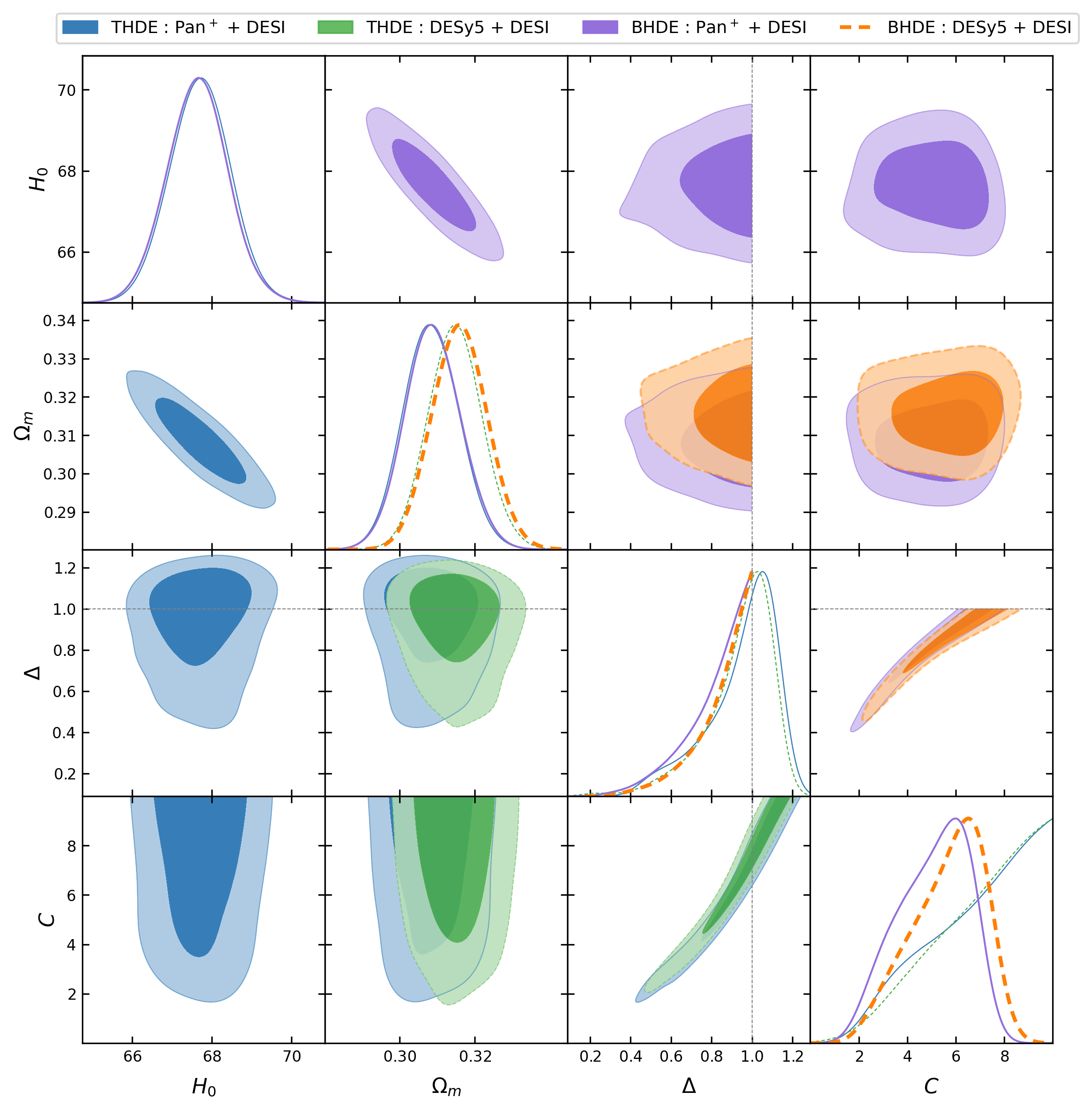
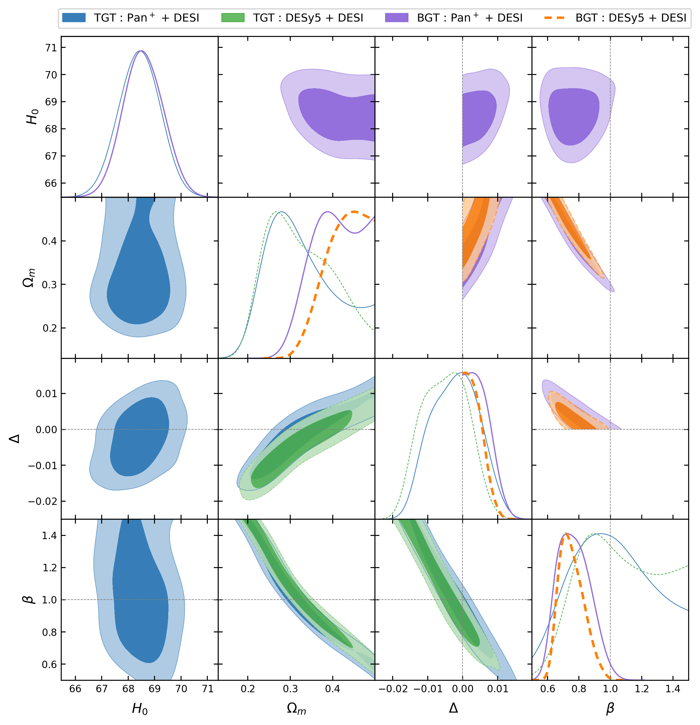
Figure 1: Contours for the $68\%$ and $95\%$ confidence limits on the Holographic Dark Energy approach (left) and the Gravity Thermodynamics approach (right), for all data combinations under considerations. The upper and lower triangle plots show the constraints when imposing the Barrow and Tsallis limits on the parameter $\Delta$, respectively.

IV Results and discussion

We begin by presenting our results for the constraints obtained for the extended models and then proceed to discuss the model selection based on Bayesian evidence. As we have described in the Section II, the essential difference between the Barrow or the Tsallis interpretation of the functional model is solely the prior ranges which define the physical viability of the model.

IV.1 Constraints

All the parameter constraints are summarized in Table 2 and Table 3, which are obtained utilising combinations of Pan⁺ and DESy5 datasets, respectively. Although we present the results using both Pan⁺and DESy5 the supernovae compilations, we mainly refer to the former for our final results, while utilising the latter for a comparative discussion as it is the most recent and latest dataset available. We first discuss the results obtained using the Holographic principle, followed by a discussion of the same using gravity-thermodynamics formalism, before presenting a comparative analysis.

Holographic principle: We find that our constraints are consistent with the limits quoted in earlier works for the BHDE Saridakis (2020); Denkiewicz et al. (2023); Dabrowski and Salzano (2020). Our results also align with other works in the context of THDE Saridakis et al. (2018); Mendoza-Martínez et al. (2024); D’Agostino (2019), where the HDE normalization parameter $C=1$ is sometimes assumed. As seen in fig. 1, when $C=1$ is imposed, our results converge to the constraints presented in these works, providing extremely tight constraints on the index parameter $\Delta$. Note that our constraints are slightly less stringent, being $\Delta>0.48$ at $2\sigma$ C.L., compared to $\Delta>0.63$ Denkiewicz et al. (2023), as we only use SNe and BAO datasets (even with the more recent DESI) and do not include very strong CMB constraints. However, it is interesting and validating that the inclusion of additional datasets such as Cosmic Chronometers Moresco et al. (2016a, b) and Strong lensing datasets Birrer et al. (2019) only mildly aid the joint constraints, while the latter prefers a slightly larger value of $\Omega_{\rm m0}$.

However, the above interpretation of consistency comes with the caveat that the posteriors are subject to the assumed prior volume. This is evident as the sampling effects on the parameter space when the prior volume is increased to that of the Tsallis bounds. On the other hand, we find an upper limit on $\Delta$ completely driven by the upper limit of $C<10$. In turn, we find that $\Delta=0$ is a disfavored scenario within both the Barrow and Tsallis priors, as presented in Denkiewicz et al. (2023), thus deviating from the standard Holographic dark energy Li (2004). It should be noted that only the BAO datasets are able to provide strong limits on $\Delta$, being constrained by the combination of both distance and expansion rate.

The constraints obtained on the parameters $\{H_{0},\Omega_{\rm m0}\}$ are completely consistent with those obtained in the $\Lambda$CDM model. While the SNe datasets alone are unable to constrain the matter density parameter $\Omega_{\rm m0}$, the BAO dataset along with the inverse distance ladder priors from CMB is able to provide a tight constraint on the parameter. Additionally, the inclusion of SH0ES calibration ($M_{\rm b}$-prior) to the SNe dataset or the $r_{\rm d}$ prior to the BAO dataset does not influence the constraints on the holographic entropy parameters. Interestingly, the HDE approach is able to solve the $H_{0}$-tension Riess et al. (2022) while satisfying the inverse distance ladder prior, aided by mildly lower values of $\Omega_{\rm m0}\sim 0.28$. However, this is disfavored when the SNe is included in the analysis, showing no advantage in solving the $H_{0}$-tension. When including the QSO dataset, we do not find any significant improvement in the constraints. Furthermore, the most recent dataset combinations of DESI+DESy5 and DESI+Pan⁺ show no difference in the constraints on the HDE parameters. However, both the inclusion of the QSO dataset and the most recent DESy5 SNe dataset provide strong implications for model selection, which is indeed the primary focus of our investigation.

Gravity-Thermodynamics: The joint analysis indicates that the cosmological parameters $H_{0}$ and $\Omega_{\rm m0}$ are consistent with the concordance cosmology. However, there is a strong degeneracy between the matter density ($\Omega_{\rm m0}$) and the normalization parameter $\beta$, as seen in the right panel of fig. 1. The range of $\beta>1.0$ prefers low values of $\Omega_{\rm m0}$, and the opposite is observed for $\beta<1$. In comparison to the results presented in Leon et al. (2021), where strong CMB priors are imposed on $\Omega_{\rm m0}$ to obtain strong constraints on $\beta$, we do not find such constraints in our analysis. As anticipated in section II.2, $\Delta\rightarrow 0$ and $\beta\to 1$ indicate that the model converges to $\Lambda$CDM cosmology. In our analysis, we find that $\beta\leq 1$ at least at a $\sim 2\sigma$ C.L. when $\Delta\to 0$, indicating a deviation from the ${\Lambda\rm{CDM}}$ model, which is also reflected in the Bayesian evidence (see section IV.2). This deviation is evident in the constraints with $\beta\sim 0.75$, as seen in table 2 and the upper triangle of the left panel in fig. 1, when the Barrow limits are adopted. When the limits on $\Delta$ are extended to the Tsallis model, $\beta\sim 1$ does obtain a posterior peak, although it remains completely unconstrained while retaining the deviation from the ${\Lambda\rm{CDM}}$ case at $\sim 2\sigma$. We find the significance of this deviation in BHDE limits to be at $1.23\sigma,2.05\sigma,3.45\sigma$ using the DESI, Pan⁺+DESI, DESy5+DESI datasets, respectively. The latter of the three data combinations is a significant deviation, being equivalent to the deviation from $\Lambda$CDM quoted in Adame et al. (2024) using phenomenological modelling of dynamical dark energy, namely the CPL Chevallier and Polarski (2001); Linder (2003) model considerations. Further discussion on this topic is provided in section IV.3.

In Barrow et al. (2021); Ghoshal and Lambiase (2021); Jizba and Lambiase (2023), limits on the exponent ($\Delta$) were placed considering the Big Bang Nucleosynthesis at early times (see also Luciano, 2023; Luciano and Giné, 2023, for limits based on inflation). In the context of the equivalent GT approach as explored here, extremely tight bounds of $\Delta\leq 1.4\times 10^{-4}$ were presented over the allowed values Barrow et al. (2021). More recently, in Luciano (2023), a less stringent limit of $\Delta\sim 0.008$ is reported, considering a similar analysis. These limits are subject to the cosmological approach followed using the $\mathcal{S}{\text{eff}}$ and are valid only within the GT approach. Also, the normalization parameter $\beta$ is usually set to unity in most of the aforementioned analyses. When imposing the Barrow limits of $\Delta>0$, we find the $95\%$ C.L. upper limit to be $\Delta<0.011$ and $\Delta<0.008$ using the Pan⁺+DESI and DESy5+DESI, respectively. We find that our constraints here are in very good agreement with the limits set in the aforementioned analyses, which consider completely different epochs. When imposing the Tsallis limits, we find that the median of the posteriors tends to $\Delta<0$ while being consistent with $\Delta\to 0$ within $1-2\sigma$ C.L. for all dataset combinations.

Comparing the HDE and GT approaches, we find $\Omega_{\rm m0}$ is better constrained in the former than in the latter, where the upper limit on the same is weakened in almost all the data combinations. Interestingly, the BGT with tighter bounds of $\Delta$ tends to push the $\Omega_{\rm m0}$ values to be larger than in the TGT case with wider $\Delta$ priors, which in turn provides no upper bound. While the HDE approach usually constrains $\Omega_{\rm m0}$, to be larger than the ${\Lambda\rm{CDM}}$ value.

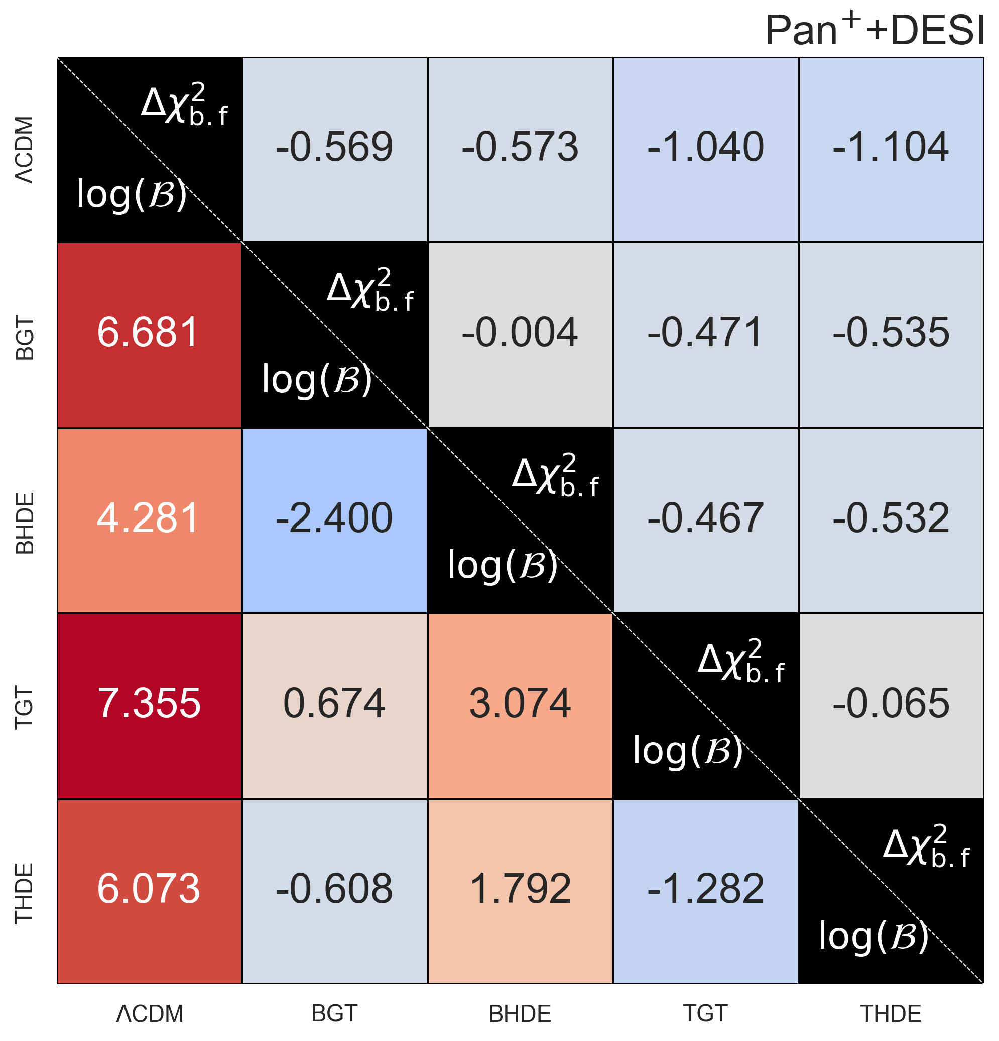
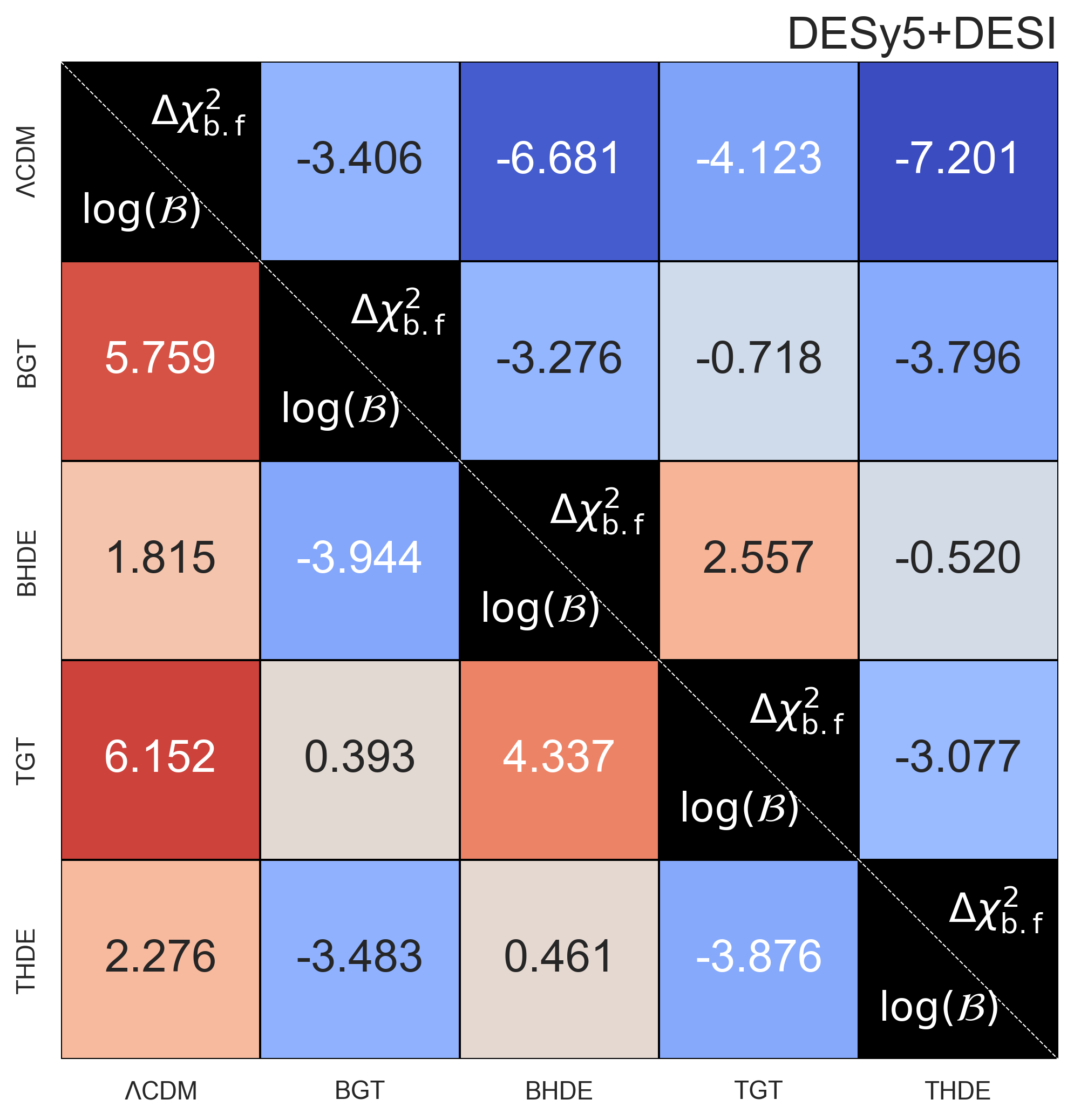
Figure 2: Comparison of the Bayesian Evidence and the best-fit $\Delta\chi^{2}$ for all the combinations of models under consideration. The left panel shows the data combination Pan⁺+ DESI and the right panel is shown for the more recent DESy5+DESI.

IV.2 Bayesian Evidence

We estimate the Bayesian evidence comparing against the ${\Lambda\rm{CDM}}$ model as presented in the last column of tables 2 and 3 and fig. 2. As anticipated, we find that the ${\Lambda\rm{CDM}}$ model is almost always preferred over the extended HDE and GT approaches both within the Barrow and Tsallis limits. However, we mainly focus on our primary motive of assessing the performance of HDE and GT Entropic approaches against each other. As can be seen from the SNe-only analysis, neither the Pan⁺nor the DESy5 is able to strongly constrain the parameters nor provide a strong preference for the ${\Lambda\rm{CDM}}$ model. SNe datasets provide maximum Bayesian evidence against the THDE model of the order $\log{\mathcal{B}}\sim 3.3$ using the Pan⁺compilation, which is moderate evidence disfavoring the model. On the other hand, the DESI dataset is consistently able to disfavour all the extended models with almost a strong significance of $\log{\mathcal{B}}\gtrsim 5$. However, in this case, the GT approaches are more strongly disfavored than the HDE approaches.

Having established the preferences of individual datasets, we now turn to the joint analysis of the SNe and BAO datasets. In fig. 2, within each heatmap, we show the comparison of the $\log{\mathcal{B}}$ and $\Delta\chi^{2}_{\rm b.f}$, in the lower and upper triangles, respectively. The values in each cell are computed as the difference between the value corresponding to the model on the x-axis wrt the respective model on the y-axis. For instance, the first column shows the difference between the Evidence for the models on the y-axis wrt ${\Lambda\rm{CDM}}$ on the x-axis, where we see that the ${\Lambda\rm{CDM}}$ is always preferred over the extension. Similarly, the top row shows that all the models on the x-axis have better $\chi^{2}_{\rm b.f}$ than that in the ${\Lambda\rm{CDM}}$ model. This is indeed what one would expect, with increasing number of parameters in the extended models they will fit the data better in terms of $\chi^{2}$. However, since the number of parameters in GT and HDE models is the same, even $\chi^{2}$ can be used to compare these two approaches. We find that these results are in line with the Bayesian evidence results i.e. $\chi^{2}_{\rm b.f}$ of the HDE model is lower than the $\Delta\chi^{2}_{\rm b.f}$ in the GT approach.

We find that the Pan⁺+DESI dataset once again disfavours all the extended models strongly, i.e., $\log{\mathcal{B}}\gtrsim 5$. The BHDE is disfavoured wrt the ${\Lambda\rm{CDM}}$ model having $\log{\mathcal{B}}\sim 4.3$, which is equivalent significance reported in Denkiewicz et al. (2023), while using a different set of data. However, very interestingly now replacing the Pan⁺with the more recent DESy5 SNe we find a clear preference for the HDE models over the GT approaches. The aforementioned significance of $\log{\mathcal{B}}\sim 4.3$ is now reduced to $\log{\mathcal{B}}\sim 1.8$ using the more recent DESI+ DESy5 dataset, implying BHDE performs very well. We find that the newer DESy5+DESI data compilations fit the HDE models with better $\Delta\chi^{2}_{\rm b.f}\sim-7$ for both the Barrow and Tsallis bounds. This, in turn, reflects positively in terms of Evidence as the HDE models can be interpreted to fit almost equivalently to the ${\Lambda\rm{CDM}}$ model. On the other hand, the GT approaches, while having slightly better $\Delta\chi^{2}_{\rm b.f}\sim-3.4$ (Barrow) and $\Delta\chi^{2}_{\rm b.f}\sim-4.1$ (Tsallis), fare extremely poorly being disfavored with $\log{\mathcal{B}}\sim 5.8$ and $\log{\mathcal{B}}\sim 6.2$ in terms of Bayesian evidence, respectively. The THDE and BHDE models, on the other hand, perform equally well as the ${\Lambda\rm{CDM}}$ model. In this context, we almost most definitely find that the HDE approach performs better than the GT approach.

In a similar way, comparing the GT approaches with the BHDE model, we find that the TGT and BGT approaches are disfavoured at $\log{\mathcal{B}}\sim 4.0$ and $\log{\mathcal{B}}\sim 4.3$, respectively, when using DESy5+DESI data. With the Pan⁺+DESI we find a moderate preference of $\log{\mathcal{B}}\sim-3.1$ for the BHDE over the TGT model. From the evidence analysis, we can also note that generally, the Barrow entropic models are mildly favoured over their corresponding Tsallis counterparts for all the combinations of datasets.

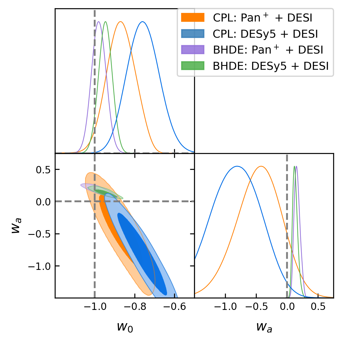
Figure 3: Contours for Barrow Holographic Dark Energy (BHDE) cosmology obtain the dataset combinations of SNe + DESI. The phenomenological CPL model is also shown for comparison.

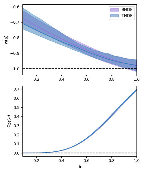
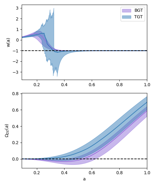
Figure 4: We show the dark energy density (top) and corresponding EoS (bottom) in both the formalisms, Gravity-Thermodynamics (left) and Holographic approach (right). The shaded region indicates the $68\%$ C.L. region.

IV.3 Dark Energy implications

We now turn to estimate the dark energy equation of state, $w(z)$ for the two entropic formalisms. As is very well known, the HDE and GT approaches provide dynamical behaviour to the dark energy density ($\Omega_{\rm HDE},\Omega_{\rm GT}$). We construct the $w(z)$ and also compute the derivative of the same to construct the $\{w_{0},w_{\rm a}\}$ parameter space. This assessment is also necessary to better understand the constraints obtained in the parameter space formally utilized when assessing deviations from the standard ${\Lambda\rm{CDM}}$ scenario. For ease of comparison, we display both the functional evolution of $w(z)$ in fig. 4 and the $w_{0}$ vs $w_{\rm a}$ parameter space (see fig. 3). As we show in fig. 3, the BHDE models are constrained in similar parameter ranges as the phenomenological CPL parameters. The larger posteriors of CPL parameter space are completely in agreement with the much tighter posteriors within the HDE model.

As shown in the top panels of fig. 4, we find that the dark energy equation of state ($\omega_{\rm GT}$) in the TGT approach shows a singularity at $z\sim 1.8$ transitioning from the $\omega_{\rm GT}(z\lesssim 1.8)\sim-1$ to $\omega_{\rm GT}(z\gtrsim 1.8)\sim 0$, consistent with ${\Lambda\rm{CDM}}$ at late-times and transitioning to a radiation-like behaviour at higher redshifts. Note that the singularity present in the TGT model is not present in the BGT model, which shows a smooth transition to the $\omega_{\rm GT}\to 0$. This is a formal assessment of the argument presented in Denkiewicz et al. (2023) that the GT approach can mimic the ${\Lambda\rm{CDM}}$ model at late times while only being a radiation correction to the standard ${\Lambda\rm{CDM}}$ model at higher redshifts. Our results for the BGT models here are in good agreement with those presented in Leon et al. (2021), where a simple freezing-like behaviour was obtained, which is also complemented by their inclusion of strong ${\Lambda\rm{CDM}}$ based CMB priors on $\Omega_{\rm m0}$ assumed therein. As found in Leon et al. (2021), for the BGT model, we find possible negative values of $\Omega_{\rm GT}$, which is not observed in the TGT approach.

On the other hand, the HDE shows a more quintessence-like behaviour mimicking a freezing field Linder (2006) with $\omega_{\rm HDE}\gtrsim-1$ at all redshifts. Note that this is in contrast to the recent claims of dynamical dark energy at higher redshifts Adame et al. (2024), where a late-time quintessence with phantom-crossing was observed using the standard Chavelier-Polarski-Linder (CPL)13 parameterization Chevallier and Polarski (2001); Linder (2003). While we do not formally compare the CPL model and our HDE model, it is evident that the HDE model is consistent with the equivalent dynamical dark energy claims within $2\sigma$ limits. We find that the $w_{0}$ estimates in all the entropic scenarios are consistent within $1\sigma$ with cosmological constant.

V Conclusions

We have implemented and assessed the viability of widely used cosmological models based on Entropic approaches implementing the ”Holographic Principle” (HDE)Li (2004) and ”Gravity - Thermodynamics” (GT) Padmanabhan (2005); Jacobson (1995) using the most recent late-time cosmological observables, namely SNe from Pan⁺Scolnic et al. (2022) and DESy5 Abbott et al. (2024) and BAO from DESI Adame et al. (2024). This is then followed by our primary objective, which is to perform model selection utilising the Bayesian evidence to asses which of the two approaches are preferred by the data. We summarize our final results as follows:

• We find the SNe datasets, both Pan⁺and DESy5, are unable to strongly disfavour the entropic approaches, performing equivalently as the ${\Lambda\rm{CDM}}$ model.

• The more recent BAO (DESI) dataset is able to provide strong evidence against the GT models while moderately disfavouring the HDE approach.

• We find that when using the combination of most recent datasets, DESI(BAO)+Pan⁺(SNe), we find that all the models are strongly disfavored, except the BHDE model, which is moderately disfavored.

• However, interestingly, using the more recent DESy5 dataset in combination with the recent DESI data, we find that the GT approaches are strongly disfavored $\log{\mathcal{B}}\gtrsim 6$. On the other hand, the HDE approach performs equivalently to the ${\Lambda\rm{CDM}}$ model.

• This establishes a clear result that amongst the entropic-based approaches to late-time cosmology, the HDE and hence the holographic principle is the preferred direction to explore given the most recent data.

• While we have not utilised the QSO as a primary dataset in our analysis, once the high-z QSO data is included, we find that the GT approach is still strongly disfavoured at $\log{\mathcal{B}}\gtrsim 5$ while the HDE fares extremely well, even providing preference wrt the ${\Lambda\rm{CDM}}$ model.

• Alongside assessing the viability of the models, we also present the dark energy constraints for the HDE and GT approaches.

• We find the HDE approaches to be consistent with simple quintessence-like behaviour without phantom crossing. The GT approach, on the other hand, does present mild phantom crossing with radiation-like behaviour at high redshift.

Entropic approaches provide a simple yet natural extension to standard cosmology based on cosmological constant. As indicated earlier in Carroll and Remmen (2016), the implementation through the Holographic principle and gravity thermodynamics conjecture differ formally. However, given the diversity in the existing possibilities, it is important to assess the possible directions that need to be explored in the future. In this context, we have attempted to contrast the HP-based applications to darker energy and modifications to cosmological constant through GT conjecture, finding a clear preference for the former. We intend to extend our current analysis to the application of more general entropy forms Nojiri et al. (2022) to cosmology. Also, in light of the more precise late-time data from EUCLID Amendola et al. (2018); Mellier et al. (2024), LSST Ivezic et al. (2019) to arrive, it is both necessary and imminent to establish viable directions to explore within the vast landscape of available entropic approaches.

Appendix A Effect of Priors on the Constraints

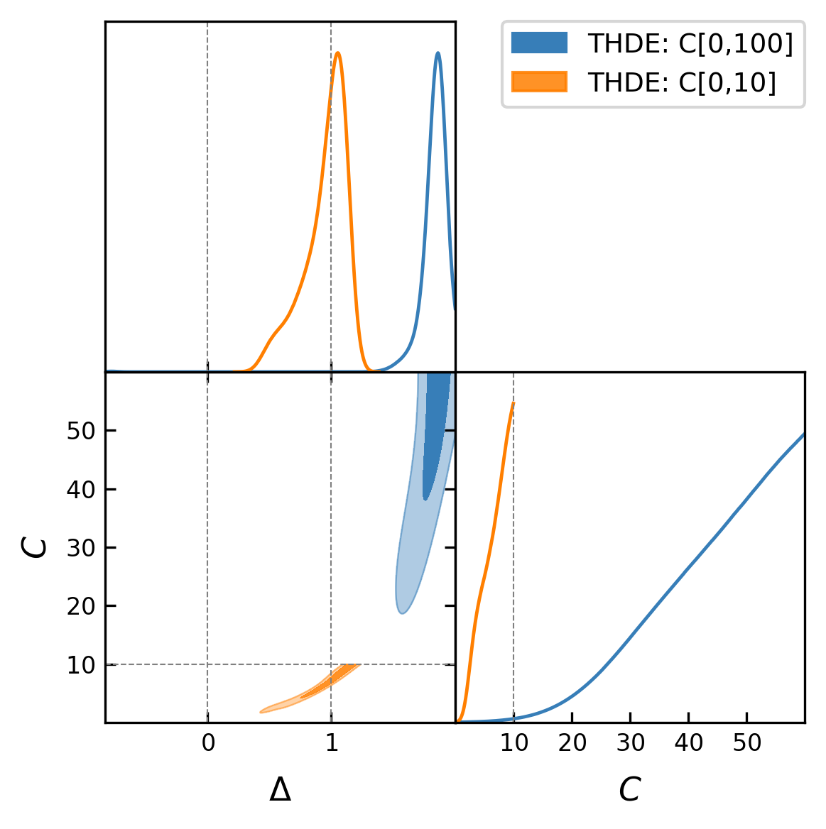
Figure 5: Contours for $68\%,95\%$ C.L., in the THDE model with varied limit son the normalisation parameter ($C$).

As we have earlier mentioned in table 1, we have utilised $C\in\{0,10\}$, in our main analysis for both THDE and BHDE models. However, as can be seen in fig. 5 when the limits are increased to $C\in\{0,100\}$, the posterior in $C\,\text{vs.}\,\Delta$ parameter space is completely beyond the limits presented in the main analysis. The case of BHDE allows for the possibility of constraining $C$ as well, guided by the limit of $\Delta<1.0$. This, however, is not true for the THDE model. Conservatively, we maintain the same limits as those used for the BHDE, which also maintains consistency in the context of comparing the Bayesian Evidence. Increasing the prior volume of THDE can additionally penalise the model while providing better $\Delta\chi^{2}_{\rm b.f}$. However, this choice of the prior does not influence our final inference that the HDE approach performs better than the gravity-thermodynamics. For instance, when using the Pan⁺+ DESI dataset, we find THDE with extended priors on $C$ to be disfavour moderately at $\log{\mathcal{B}}\sim 3.48$, in contrast to the strong evidence of $\log{\mathcal{B}}\sim 6.07$ (see table 2) obtained against the model in the main analysis.

Appendix B Tables of constraints and contour plots

For brevity in the main text, we show our tables of constraints, here in the appendix.

Table 2: Constraints (68% C.L.) on the free model parameters of the entropic models and the ${\Lambda\rm{CDM}}$ model. We compare here the constraints using the datasets Pan⁺(SNe), DESI (BAO) and Quasar compilation. The parameter $H_{0}$ is measured in units of km/s Mpc^-1. Here joint implies Pan⁺+ DESI + QSO. In the last column, we show the Bayesian evidence for each model computed against the ${\Lambda\rm{CDM}}$ model. We remind that in our comparison a positive value of $\log{\mathcal{B}}$ implies that the model in comparison is disfavored wrt ${\Lambda\rm{CDM}}$ model.

Dataset	Model	$\Omega_{\rm m}$	$H_{0}$	$\Delta$	$C/\beta$	$M_{b}$	$r_{d}$	$\log{\mathcal{B}}$
Pan+	${\Lambda\rm{CDM}}$	$0.332_{-0.018}^{+0.018}$	$73.250_{-0.995}^{+1.021}$	$-$	$-$	$-19.252_{-0.029}^{+0.029}$	$-$	$0$
	BGT	$>0.243$	$73.309_{-0.941}^{+1.011}$	$<0.627$	$>0.725$	$-19.253_{-0.027}^{+0.029}$	$-$	$2.154$
	BHDE	$0.249_{-0.062}^{+0.057}$	$73.154_{-1.041}^{+1.040}$	$>0.282$	$>2.09$	$-19.250_{-0.029}^{+0.030}$	$-$	$1.936$
	TGT	$--$	$73.136_{-0.980}^{+0.986}$	$-0.411_{-0.441}^{+0.473}$	$--$	$-19.254_{-0.028}^{+0.029}$	$-$	$2.354$
	THDE	$0.253_{-0.070}^{+0.062}$	$73.020_{-0.955}^{+1.039}$	$0.674_{-0.459}^{+0.281}$	$--$	$-19.255_{-0.027}^{+0.029}$	$-$	$3.329$
DESI	${\Lambda\rm{CDM}}$	$0.296_{-0.007}^{+0.007}$	$69.187_{-0.615}^{+0.649}$	$-$	$-$	$-$	$147.263_{-0.323}^{+0.334}$	$0$
	BGT	$>0.263$	$69.743_{-0.948}^{+0.941}$	$<0.016$	$0.762_{-0.128}^{+0.194}$	$-$	$147.254_{-0.336}^{+0.329}$	$6.453$
	BHDE	$0.280_{-0.024}^{+0.022}$	$71.065_{-2.724}^{+3.355}$	$>0.241$	$3.777_{-1.961}^{+1.655}$	$-$	$147.284_{-0.312}^{+0.348}$	$4.129$
	TGT	$0.320_{-0.085}^{+0.101}$	$69.525_{-0.973}^{+0.983}$	$0.003_{-0.009}^{+0.008}$	$--$	$-$	$147.236_{-0.339}^{+0.340}$	$7.471$
	THDE	$0.278_{-0.025}^{+0.021}$	$71.365_{-2.640}^{+3.489}$	$0.960_{-0.352}^{+0.208}$	$--$	$-$	$147.280_{-0.364}^{+0.344}$	$5.022$
Pan++DESI	${\Lambda\rm{CDM}}$	$0.301_{-0.006}^{+0.006}$	$68.825_{-0.610}^{+0.583}$	$-$	$-$	$-19.398_{-0.018}^{+0.017}$	$147.149_{-0.317}^{+0.323}$	$0$
	BGT	$>0.314$	$68.566_{-0.740}^{+0.781}$	$<0.011$	$0.764_{-0.106}^{+0.115}$	$-19.405_{-0.020}^{+0.021}$	$147.228_{-0.332}^{+0.331}$	$6.681$
	BHDE	$0.309_{-0.007}^{+0.007}$	$67.673_{-0.778}^{+0.694}$	$>0.502$	$5.253_{-1.984}^{+1.386}$	$-19.427_{-0.020}^{+0.018}$	$147.330_{-0.339}^{+0.357}$	$4.281$
	TGT	$>0.218$	$68.446_{-0.794}^{+0.777}$	$-0.002_{-0.008}^{+0.007}$	$--$	$-19.407_{-0.022}^{+0.021}$	$147.258_{-0.340}^{+0.341}$	$7.355$
	THDE	$0.308_{-0.007}^{+0.008}$	$67.698_{-0.794}^{+0.715}$	$0.988_{-0.356}^{+0.124}$	$>0.279$	$-19.426_{-0.020}^{+0.019}$	$147.328_{-0.343}^{+0.319}$	$6.073$
Joint	${\Lambda\rm{CDM}}$	$0.304_{-0.006}^{+0.006}$	$68.593_{-0.585}^{+0.600}$	$-$	$-$	$-19.404_{-0.018}^{+0.018}$	$147.085_{-0.327}^{+0.325}$	$0$
	BGT	$>0.351$	$68.003_{-0.734}^{+0.763}$	$<0.009$	$0.740_{-0.071}^{+0.091}$	$-19.419_{-0.020}^{+0.021}$	$147.238_{-0.319}^{+0.328}$	$6.181$
	BHDE	$0.312_{-0.008}^{+0.008}$	$67.356_{-0.727}^{+0.825}$	$>0.482$	$4.927_{-1.735}^{+1.615}$	$-19.434_{-0.019}^{+0.021}$	$147.282_{-0.325}^{+0.344}$	$2.885$
	TGT	$0.262_{-0.032}^{+0.051}$	$67.734_{-0.734}^{+0.710}$	$-0.009_{-0.005}^{+0.005}$	$>0.932$	$-19.425_{-0.021}^{+0.020}$	$147.253_{-0.346}^{+0.329}$	$6.996$
	THDE	$0.312_{-0.008}^{+0.008}$	$67.352_{-0.759}^{+0.768}$	$0.783_{-0.401}^{+0.274}$	$--$	$-19.435_{-0.019}^{+0.020}$	$147.309_{-0.352}^{+0.315}$	$3.395$

Table 3: Same as table 2, replacing the SNe compilation from Pan⁺to DESy5. In contrast to table 2, we do not have the $M_{\rm b}$ in the DESy5 constraints.

Dataset	Model	$\Omega_{\rm m}$	$H_{0}$	$\Delta$	$C/\beta$	$M_{b}$	$r_{d}$	$\log{\mathcal{B}}$
DESy5	${\Lambda\rm{CDM}}$	$0.353_{-0.017}^{+0.017}$	$69.481_{-19.853}^{+20.840}$	$-$	$-$	$-$	$-$	$0$
	BGT	$>0.256$	$69.693_{-20.261}^{+20.854}$	$<0.776$	$>0.775$	$-$	$-$	$1.842$
	BHDE	$<0.324$	$69.128_{-19.716}^{+20.347}$	$--$	$>1.9$	$-$	$-$	$0.932$
	TGT	$--$	$70.558_{-20.380}^{+20.001}$	$-0.502_{-0.519}^{+0.570}$	$--$	$-$	$-$	$2.018$
	THDE	$<0.332$	$66.345_{-18.780}^{+22.919}$	$0.573_{-0.546}^{+0.386}$	$--$	$-$	$-$	$2.568$
DESy5+DESI	${\Lambda\rm{CDM}}$	$0.305_{-0.006}^{+0.006}$	$69.488_{-0.568}^{+0.589}$	$-$	$-$	$-$	$147.067_{-0.329}^{+0.326}$	$0$
	BGT	$>0.346$	$67.893_{-0.692}^{+0.720}$	$<0.008$	$0.743_{-0.068}^{+0.094}$	$-$	$147.251_{-0.334}^{+0.343}$	$5.759$
	BHDE	$0.316_{-0.007}^{+0.007}$	$66.891_{-0.729}^{+0.700}$	$>0.565$	$5.901_{-2.055}^{+1.290}$	$-$	$147.352_{-0.337}^{+0.324}$	$1.815$
	TGT	$0.311_{-0.073}^{+0.098}$	$67.722_{-0.716}^{+0.726}$	$-0.005_{-0.007}^{+0.007}$	$>0.709$	$-$	$147.225_{-0.338}^{+0.339}$	$6.152$
	THDE	$0.315_{-0.007}^{+0.007}$	$67.028_{-0.726}^{+0.715}$	$0.987_{-0.212}^{+0.104}$	$>3.12$	$-$	$147.319_{-0.311}^{+0.339}$	$2.276$
Joint	${\Lambda\rm{CDM}}$	$0.308_{-0.006}^{+0.006}$	$68.245_{-0.561}^{+0.601}$	$-$	$-$	$-$	$146.984_{-0.333}^{+0.326}$	$0$
	BGT	$>0.362$	$67.498_{-0.690}^{+0.711}$	$<0.006$	$0.748_{-0.059}^{+0.073}$	$-$	$147.211_{-0.328}^{+0.340}$	$4.362$
	BHDE	$0.319_{-0.007}^{+0.007}$	$66.620_{-0.727}^{+0.723}$	$--$	$5.348_{-2.580}^{+1.724}$	$-$	$147.297_{-0.316}^{+0.338}$	$-0.466$
	TGT	$0.291_{-0.046}^{+0.065}$	$67.174_{-0.701}^{+0.680}$	$-0.009_{-0.006}^{+0.006}$	$>0.843$	$-$	$147.238_{-0.334}^{+0.324}$	$5.095$
	THDE	$0.318_{-0.007}^{+0.007}$	$66.640_{-0.669}^{+0.689}$	$0.924_{-0.331}^{+0.148}$	$>2.32$	$-$	$147.311_{-0.342}^{+0.306}$	$0.609$

References

- Riess et al. (1998) A. G. Riess et al. (Supernova Search Team), Astron. J. 116, 1009 (1998), arXiv:astro-ph/9805201 [astro-ph] .
- Betoule et al. (2014) M. Betoule et al. (SDSS), Astron. Astrophys. 568, A22 (2014), arXiv:1401.4064 [astro-ph.CO] .
- Scolnic et al. (2018) D. M. Scolnic et al., Astrophys. J. 859, 101 (2018), arXiv:1710.00845 [astro-ph.CO] .
- Scolnic et al. (2022) D. Scolnic et al., Astrophys. J. 938, 113 (2022), arXiv:2112.03863 [astro-ph.CO] .
- Haridasu et al. (2018a) B. S. Haridasu, V. V. Luković, and N. Vittorio, J. Cosmology Astropart. Phys. 5, 033 (2018a), arXiv:1711.03929 .
- Abbott et al. (2024) T. M. C. Abbott et al. (DES), (2024), arXiv:2401.02929 [astro-ph.CO] .
- Dam et al. (2017) L. H. Dam, A. Heinesen, and D. L. Wiltshire, Mon. Not. Roy. Astron. Soc. 472, 835 (2017), arXiv:1706.07236 [astro-ph.CO] .
- Rubin and Hayden (2016) D. Rubin and B. Hayden, Astrophys. J. Lett. 833, L30 (2016), arXiv:1610.08972 [astro-ph.CO] .
- Ade et al. (2016) P. A. R. Ade et al. (Planck), Astron. Astrophys. 594, A24 (2016), arXiv:1502.01597 [astro-ph.CO] .
- Aghanim et al. (2020) N. Aghanim et al. (Planck), Astron. Astrophys. 641, A6 (2020), [Erratum: Astron.Astrophys. 652, C4 (2021)], arXiv:1807.06209 [astro-ph.CO] .
- Verde et al. (2019) L. Verde, T. Treu, and A. G. Riess, in Nature Astronomy 2019 (2019) arXiv:1907.10625 [astro-ph.CO] .
- Riess et al. (2022) A. G. Riess et al., Astrophys. J. Lett. 934, L7 (2022), arXiv:2112.04510 [astro-ph.CO] .
- Riess (2019) A. G. Riess, Nature Rev. Phys. 2, 10 (2019), arXiv:2001.03624 [astro-ph.CO] .
- Abdalla et al. (2022) E. Abdalla et al., JHEAp 34, 49 (2022), arXiv:2203.06142 [astro-ph.CO] .
- Perivolaropoulos and Skara (2022) L. Perivolaropoulos and F. Skara, New Astron. Rev. 95, 101659 (2022), arXiv:2105.05208 [astro-ph.CO] .
- Efstathiou (2020) G. Efstathiou, (2020), arXiv:2007.10716 [astro-ph.CO] .
- Freedman (2021) W. L. Freedman, Astrophys. J. 919, 16 (2021), arXiv:2106.15656 [astro-ph.CO] .
- Verde et al. (2023) L. Verde, N. Schöneberg, and H. Gil-Marín, (2023), arXiv:2311.13305 [astro-ph.CO] .
- Wang et al. (2017a) S. Wang, Y. Wang, and M. Li, Phys. Rept. 696, 1 (2017a), arXiv:1612.00345 [astro-ph.CO] .
- del Campo et al. (2011) S. del Campo, J. C. Fabris, R. Herrera, and W. Zimdahl, Phys. Rev. D 83, 123006 (2011).
- Saridakis et al. (2018) E. N. Saridakis, K. Bamba, R. Myrzakulov, and F. K. Anagnostopoulos, Journal of Cosmology and Astroparticle Physics 2018, 012 (2018).
- Nojiri et al. (2021) S. Nojiri, S. D. Odintsov, and T. Paul, Symmetry 13, 928 (2021), arXiv:2105.08438 [gr-qc] .
- ’t Hooft (1993) G. ’t Hooft, Conf. Proc. C 930308, 284 (1993), arXiv:gr-qc/9310026 .
- Susskind (1995) L. Susskind, J. Math. Phys. 36, 6377 (1995), arXiv:hep-th/9409089 .
- Bekenstein (1994) J. D. Bekenstein, Phys. Rev. D 49, 1912 (1994), arXiv:gr-qc/9307035 .
- Nappi and Pasquinucci (1992) C. R. Nappi and A. Pasquinucci, Mod. Phys. Lett. A 7, 3337 (1992), arXiv:gr-qc/9208002 .
- Carlip (2014) S. Carlip, Int. J. Mod. Phys. D 23, 1430023 (2014), arXiv:1410.1486 [gr-qc] .
- Brown (1994) J. D. Brown, (1994), arXiv:gr-qc/9404006 .
- Oda (1994) I. Oda, Phys. Lett. B 338, 165 (1994), arXiv:hep-th/9405185 .
- Ghosh and Mitra (1996) A. Ghosh and P. Mitra, Mod. Phys. Lett. A 11, 1231 (1996), arXiv:gr-qc/9408040 .
- Frolov (1995) V. P. Frolov, Phys. Rev. Lett. 74, 3319 (1995), arXiv:gr-qc/9406037 .
- Fursaev (1995) D. V. Fursaev, Mod. Phys. Lett. A 10, 649 (1995), arXiv:hep-th/9408066 .
- Louko and Whiting (1995) J. Louko and B. F. Whiting, Phys. Rev. D 51, 5583 (1995), arXiv:gr-qc/9411017 .
- Liberati (1997) S. Liberati, Nuovo Cim. B 112, 405 (1997), arXiv:gr-qc/9601032 .
- Solodukhin (1996) S. N. Solodukhin, Phys. Rev. D 54, 3900 (1996), arXiv:hep-th/9601154 .
- Carlip (1997) S. Carlip, Astrophys. Space Sci. Libr. 211, 35 (1997), arXiv:gr-qc/9603049 .
- Frolov et al. (1996) V. P. Frolov, D. V. Fursaev, and A. I. Zelnikov, Phys. Lett. B 382, 220 (1996), arXiv:hep-th/9603175 .
- Quevedo et al. (2024) H. Quevedo, M. N. Quevedo, and A. Sanchez, (2024), arXiv:2405.04474 [gr-qc] .
- Bekenstein (1973) J. D. Bekenstein, Phys. Rev. D 7, 2333 (1973).
- Bekenstein (1972) J. D. Bekenstein, Lett. Nuovo Cim. 4, 737 (1972).
- Hawking (1974) S. W. Hawking, Nature 248, 30 (1974).
- Hawking (1975) S. W. Hawking, Commun. Math. Phys. 43, 199 (1975), [Erratum: Commun.Math.Phys. 46, 206 (1976)].
- Hsu (2004a) S. D. H. Hsu, Phys. Lett. B 594, 13 (2004a), arXiv:hep-th/0403052 .
- Oliveros et al. (2022) A. Oliveros, M. A. Sabogal, and M. A. Acero, Eur. Phys. J. Plus 137, 783 (2022), arXiv:2203.14464 [gr-qc] .
- Bhardwaj et al. (2022) V. K. Bhardwaj, P. Garg, A. Pradhan, and S. Krishnannair, Chin. J. Phys. 79, 471 (2022), arXiv:2207.00968 [gr-qc] .
- Astashenok and Tepliakov (2022) A. V. Astashenok and A. S. Tepliakov, Int. J. Geom. Meth. Mod. Phys. 19, 2250234 (2022), arXiv:2208.13320 [gr-qc] .
- Astashenok and Tepliakov (2023) A. V. Astashenok and A. S. Tepliakov, Int. J. Mod. Phys. D 32, 2350058 (2023), arXiv:2305.10573 [gr-qc] .
- Tita et al. (2024) A. Tita, B. Gumjudpai, and P. Srisawad, (2024), arXiv:2402.18604 [gr-qc] .
- Salzano et al. (2017) V. Salzano, D. F. Mota, S. Capozziello, and M. Donahue, Phys. Rev. D 95, 044038 (2017), arXiv:1701.03517 [astro-ph.CO] .
- Saridakis (2020) E. N. Saridakis, Journal of Cosmology and Astroparticle Physics 2020, 031–031 (2020).
- Leon et al. (2021) G. Leon, J. Magaña, A. Hernández-Almada, M. A. García-Aspeitia, T. Verdugo, and V. Motta, Journal of Cosmology and Astroparticle Physics 2021, 032 (2021).
- Cai and Kim (2005) R.-G. Cai and S. P. Kim, JHEP 02, 050 (2005), arXiv:hep-th/0501055 .
- Asghari et al. (2024) M. Asghari, A. Allahyari, and D. F. Mota, (2024), arXiv:2404.13025 [gr-qc] .
- Hawking (1976) S. W. Hawking, Phys. Rev. D 13, 191 (1976).
- Tsallis and Cirto (2013) C. Tsallis and L. J. L. Cirto, The European Physical Journal C 73 (2013), 10.1140/epjc/s10052-013-2487-6.
- Tsallis (1988) C. Tsallis, Journal of statistical physics 52, 479 (1988).
- Ré (1960) Fourth Berkeley symposium on mathematical statistics and probability 1, 547 (1960).
- Barrow (2020a) J. D. Barrow, Phys. Lett. B 808, 135643 (2020a), arXiv:2004.09444 [gr-qc] .
- Sharma and Mittal (1975) B. Sharma and D. Mittal, J. Math. Sci 10, 28 (1975).
- Sharma and Mittal (1977) B. Sharma and D. Mittal, Journal of Combinatorics Information & System Sciences 2, 122 (1977).
- Kaniadakis (2005) G. Kaniadakis, Phys. Rev. E 72, 036108 (2005), arXiv:cond-mat/0507311 .
- Nojiri et al. (2022) S. Nojiri, S. D. Odintsov, and V. Faraoni, Phys. Rev. D 105, 044042 (2022), arXiv:2201.02424 [gr-qc] .
- Ourabah (2024) K. Ourabah, Class. Quant. Grav. 41, 015010 (2024), arXiv:2306.09540 [gr-qc] .
- Odintsov et al. (2023) S. D. Odintsov, S. D’Onofrio, and T. Paul, Phys. Dark Univ. 42, 101277 (2023), arXiv:2306.15225 [gr-qc] .
- Naeem and Bibi (2024) M. Naeem and A. Bibi, Annals Phys. 462, 169618 (2024), arXiv:2308.02936 [gr-qc] .
- Nakarachinda et al. (2023) R. Nakarachinda, C. Pongkitivanichkul, D. Samart, L. Tannukij, and P. Wongjun, (2023), arXiv:2312.16901 [gr-qc] .
- Fazlollahi (2023) H. R. Fazlollahi, Eur. Phys. J. C 83, 29 (2023), arXiv:2208.12048 [gr-qc] .
- Kord Zangeneh and Sheykhi (2023) M. Kord Zangeneh and A. Sheykhi, (2023), arXiv:2311.01969 [gr-qc] .
- Salehi (2023) A. Salehi, (2023), arXiv:2309.15956 [gr-qc] .
- Barrow (2020b) J. D. Barrow, Physics Letters B 808, 135643 (2020b).
- Srednicki (1993) M. Srednicki, Phys. Rev. Lett. 71, 666 (1993), arXiv:hep-th/9303048 .
- Jacobson (2016) T. Jacobson, Phys. Rev. Lett. 116, 201101 (2016), arXiv:1505.04753 [gr-qc] .
- Jacobson (1995) T. Jacobson, Phys. Rev. Lett. 75, 1260 (1995), arXiv:gr-qc/9504004 .
- Padmanabhan (2005) T. Padmanabhan, Phys. Rept. 406, 49 (2005), arXiv:gr-qc/0311036 .
- Carroll and Remmen (2016) S. M. Carroll and G. N. Remmen, Phys. Rev. D 93, 124052 (2016), arXiv:1601.07558 [hep-th] .
- Li (2004) M. Li, Physics Letters B 603, 1–5 (2004).
- Wang et al. (2017b) S. Wang, Y. Wang, and M. Li, Physics Reports 696, 1 (2017b), holographic Dark Energy.
- Padmanabhan (2010) T. Padmanabhan, Rept. Prog. Phys. 73, 046901 (2010), arXiv:0911.5004 [gr-qc] .
- Adame et al. (2024) A. G. Adame et al. (DESI), (2024), arXiv:2404.03002 [astro-ph.CO] .
- Risaliti and Lusso (2019) G. Risaliti and E. Lusso, Nature Astron. 3, 272 (2019), arXiv:1811.02590 [astro-ph.CO] .
- Barrow (2020c) J. D. Barrow, Physics Letters B 808, 135643 (2020c).
- Denkiewicz et al. (2023) T. Denkiewicz, V. Salzano, and M. P. Dabrowski, Phys. Rev. D 108, 103533 (2023), arXiv:2303.11680 [astro-ph.CO] .
- Hsu (2004b) S. D. Hsu, Physics Letters B 594, 13–16 (2004b).
- Davis and Lineweaver (2004) T. M. Davis and C. H. Lineweaver, Publ. Astron. Soc. Austral. 21, 97 (2004), arXiv:astro-ph/0310808 .
- Dabrowski and Salzano (2020) M. P. Dabrowski and V. Salzano, Phys. Rev. D 102, 064047 (2020), arXiv:2009.08306 [astro-ph.CO] .
- Pavon and Zimdahl (2005) D. Pavon and W. Zimdahl, Phys. Lett. B 628, 206 (2005), arXiv:gr-qc/0505020 .
- Haridasu et al. (2018b) B. S. Haridasu, V. V. Luković, M. Moresco, and N. Vittorio, JCAP 1810, 015 (2018b), arXiv:1805.03595 [astro-ph.CO] .
- Gómez-Valent and Amendola (2018) A. Gómez-Valent and L. Amendola, J. Cosmology Astropart. Phys. 2018, 051 (2018), arXiv:1802.01505 [astro-ph.CO] .
- Möller et al. (2024) A. Möller et al. (DES), (2024), arXiv:2402.18690 [astro-ph.CO] .
- Alam et al. (2017) S. Alam et al. (BOSS), Mon. Not. Roy. Astron. Soc. 470, 2617 (2017), arXiv:1607.03155 [astro-ph.CO] .
- Zhao et al. (2019) G.-B. Zhao et al. (eBOSS), Mon. Not. Roy. Astron. Soc. 482, 3497 (2019), arXiv:1801.03043 [astro-ph.CO] .
- du Mas des Bourboux et al. (2020) H. du Mas des Bourboux et al. (eBOSS), Astrophys. J. 901, 153 (2020), arXiv:2007.08995 [astro-ph.CO] .
- Risaliti and Lusso (2015) G. Risaliti and E. Lusso, Astrophys. J. 815, 33 (2015), arXiv:1505.07118 .
- Lusso et al. (2020) E. Lusso et al., Astron. Astrophys. 642, A150 (2020), arXiv:2008.08586 [astro-ph.GA] .
- Li et al. (2021) X. Li, R. E. Keeley, A. Shafieloo, X. Zheng, S. Cao, M. Biesiada, and Z.-H. Zhu, Mon. Not. Roy. Astron. Soc. 507, 919 (2021), arXiv:2103.16032 [astro-ph.CO] .
- Bargiacchi et al. (2023) G. Bargiacchi, M. G. Dainotti, and S. Capozziello, Mon. Not. Roy. Astron. Soc. 525, 3104 (2023), arXiv:2307.15359 [astro-ph.CO] .
- Dainotti et al. (2023) M. G. Dainotti, G. Bargiacchi, M. Bogdan, A. L. Lenart, K. Iwasaki, S. Capozziello, B. Zhang, and N. Fraija, Astrophys. J. 951, 63 (2023), arXiv:2305.10030 [astro-ph.CO] .
- Shakura and Sunyaev (1973) N. I. Shakura and R. A. Sunyaev, Astron. Astrophys. 24, 337 (1973).
- Avni and Tananbaum (1986) Y. Avni and H. Tananbaum, Astrophys. J. 305, 83 (1986).
- Wang and Mukherjee (2006) Y. Wang and P. Mukherjee, Astrophys. J. 650, 1 (2006), arXiv:astro-ph/0604051 [astro-ph] .
- Wang and Mukherjee (2007) Y. Wang and P. Mukherjee, Phys. Rev. D 76, 103533 (2007), arXiv:astro-ph/0703780 [astro-ph] .
- Verde et al. (2017) L. Verde, E. Bellini, C. Pigozzo, A. F. Heavens, and R. Jimenez, Journal of Cosmology and Astro-Particle Physics 2017, 023 (2017), arXiv:1611.00376 [astro-ph.CO] .
- Haridasu et al. (2021) B. S. Haridasu, M. Viel, and N. Vittorio, Phys. Rev. D 103, 063539 (2021), arXiv:2012.10324 [astro-ph.CO] .
- Fixsen (2009) D. J. Fixsen, Astrophys. J. 707, 916 (2009), arXiv:0911.1955 [astro-ph.CO] .
- Foreman-Mackey et al. (2013) D. Foreman-Mackey, D. W. Hogg, D. Lang, and J. Goodman, PASP 125, 306 (2013), arXiv:1202.3665 [astro-ph.IM] .
- Lewis (2019) A. Lewis, (2019), arXiv:1910.13970 [astro-ph.IM] .
- Trotta (2017) R. Trotta (2017) arXiv:1701.01467 [astro-ph.CO] .
- Trotta (2008) R. Trotta, Contemp. Phys. 49, 71 (2008), arXiv:0803.4089 [astro-ph] .
- Haridasu et al. (2018c) B. S. Haridasu, V. V. Luković, and N. Vittorio, JCAP 1805, 033 (2018c), arXiv:1711.03929 [astro-ph.CO] .
- Heavens et al. (2017) A. Heavens, Y. Fantaye, A. Mootoovaloo, H. Eggers, Z. Hosenie, S. Kroon, and E. Sellentin, (2017), arXiv:1704.03472 [stat.CO] .
- Jeffreys (1998) H. Jeffreys, The Theory of Probability, Oxford Classic Texts in the Physical Sciences (OUP Oxford, 1998).
- Kass and Raftery (1995) R. E. Kass and A. E. Raftery, Journal of the American Statistical Association 90, 773 (1995).
- Nesseris and Garcia-Bellido (2013) S. Nesseris and J. Garcia-Bellido, JCAP 08, 036 (2013), arXiv:1210.7652 [astro-ph.CO] .
- Mendoza-Martínez et al. (2024) M. L. Mendoza-Martínez, A. Cervantes-Contreras, J. J. Trejo-Alonso, and A. Hernandez-Almada, (2024), arXiv:2404.18346 [astro-ph.CO] .
- D’Agostino (2019) R. D’Agostino, Phys. Rev. D 99, 103524 (2019), arXiv:1903.03836 [gr-qc] .
- Moresco et al. (2016a) M. Moresco, R. Jimenez, L. Verde, A. Cimatti, L. Pozzetti, C. Maraston, and D. Thomas, J. Cosmology Astropart. Phys. 12, 039 (2016a), arXiv:1604.00183 .
- Moresco et al. (2016b) M. Moresco, L. Pozzetti, A. Cimatti, R. Jimenez, C. Maraston, L. Verde, D. Thomas, A. Citro, R. Tojeiro, and D. Wilkinson, JCAP 1605, 014 (2016b), arXiv:1601.01701 [astro-ph.CO] .
- Birrer et al. (2019) S. Birrer et al., Mon. Not. Roy. Astron. Soc. 484, 4726 (2019), arXiv:1809.01274 [astro-ph.CO] .
- Chevallier and Polarski (2001) M. Chevallier and D. Polarski, Int. J. Mod. Phys. D 10, 213 (2001), arXiv:gr-qc/0009008 .
- Linder (2003) E. V. Linder, Phys. Rev. Lett. 90, 091301 (2003), arXiv:astro-ph/0208512 .
- Barrow et al. (2021) J. D. Barrow, S. Basilakos, and E. N. Saridakis, Phys. Lett. B 815, 136134 (2021), arXiv:2010.00986 [gr-qc] .
- Ghoshal and Lambiase (2021) A. Ghoshal and G. Lambiase, (2021), arXiv:2104.11296 [astro-ph.CO] .
- Jizba and Lambiase (2023) P. Jizba and G. Lambiase, Entropy 25, 1495 (2023), arXiv:2310.19045 [gr-qc] .
- Luciano (2023) G. G. Luciano, Eur. Phys. J. C 83, 329 (2023), arXiv:2301.12509 [gr-qc] .
- Luciano and Giné (2023) G. G. Luciano and J. Giné, Phys. Dark Univ. 41, 101256 (2023), arXiv:2210.09755 [gr-qc] .
- Linder (2006) E. V. Linder, Phys. Rev. D73, 063010 (2006), arXiv:astro-ph/0601052 [astro-ph] .
- Amendola et al. (2018) L. Amendola et al., Living Rev. Rel. 21, 2 (2018), arXiv:1606.00180 [astro-ph.CO] .
- Mellier et al. (2024) Y. Mellier et al. (Euclid, Isaac Newton Group of Telescopes, Apartado 321, 38700 Santa Cruz de La Palma, Spain, Astrophysics Group, Blackett Laboratory, Imperial College London, London SW7 2AZ, UK, ASDEX Upgrade Team, Max-Planck-Institut fur Plasmaphysik, Garching, Germany, MTA-CSFK Lendület Large-Scale Structure Research Group, Konkoly-Thege Miklós út 15-17, H-1121 Budapest, Hungary, NOVA optical infrared instrumentation group at ASTRON, Oude Hoogeveensedijk 4, 7991PD, Dwingeloo, The Netherlands), (2024), arXiv:2405.13491 [astro-ph.CO] .
- Ivezic et al. (2019) e. Ivezic et al. (LSST), Astrophys. J. 873, 111 (2019), arXiv:0805.2366 [astro-ph] .