remarkRemark \newsiamremarkhypothesisHypothesis \newsiamthmclaimClaim \headersJ. I. Polanco
Fast and accurate evaluation of Biot–Savart integrals over spatial curves
Abstract
The Biot–Savart law is relevant in physical contexts including electromagnetism and fluid dynamics. In the latter case, when the rotation of a fluid is confined to a set of very thin vortex filaments, this law describes the velocity field induced by the spatial arrangement of these objects. The Biot–Savart law is at the core of vortex methods used in the simulation of classical and quantum fluid flows. Naïve methods are inefficient when dealing with large numbers of vortex elements, which makes them inadequate for simulating turbulent vortex flows. Here we exploit a direct analogy between the Biot–Savart law and electrostatics to adapt Ewald summation methods, routinely used in molecular dynamics simulations, to vortex filament simulations in three-dimensional periodic domains. In this context, the basic idea is to split the induced velocity onto (i) a coarse-grained velocity generated by a Gaussian-filtered vorticity field, and (ii) a short-range correction accounting for near-singular behaviour near the vortices. The former component can be accurately and efficiently evaluated using the nonuniform fast Fourier transform algorithm. Analytical accuracy estimates are provided as a function of the parameters entering the method. We also discuss how to properly account for the finite vortex core size in kinetic energy estimations. Using numerical experiments, we verify the accuracy and the conservation properties of the proposed approach. Moreover, we demonstrate the complexity of the method over a wide range of problem sizes , considerably better than the cost of a naïve approach.
keywords:
Biot–Savart, Ewald summation, nonuniform fast Fourier transform, vortex filament model, quantum vortices65D07, 65L05, 70H05, 76B47, 76M23, 76Y05
1 Introduction
The Biot–Savart law is well known for describing the magnetic field generated by a steady electric current. It is also very relevant in fluid dynamics, where it allows to obtain the fluid velocity induced by a known vorticity field. We are interested here in the specific case where the electric current or the vorticity field are confined to spatial curves in three-dimensional space. This is a commonly encountered problem in undergraduate electromagnetism lectures, where the question is what is the magnetic field induced by a current flowing through a thin conducting wire. In the fluid dynamics case, the equivalent would be a very thin vortex filament, which can be a reasonable idealised model for vortices found in the flow of viscous fluids such as water or air. In fact, it is also a very accurate description of vortices in certain superfluids such as liquid helium-4 near the absolute zero, where rotational motion is confined to so-called quantum vortices of atomic-size thickness (the vortex core radius is ), and the circulation (or strength) of each vortex takes a constant value dictated by quantum mechanical constraints. The velocity induced at a point away from a vortex core is then given by the Biot–Savart law,
| (1) |
where denotes one or more oriented curves representing the vortex filament geometry, and denotes a vortex location.
In classical fluid dynamics, the Biot–Savart law is at the core of vortex methods [Cottet2000, Koumoutsakos2005] used to describe incompressible viscous flows. These are commonly used in aerodynamics applications [Vermeer2003], but have also been applied to problems as varied as the simulation of self-propelled swimmers in viscous fluids [Gazzola2014]. Note that, in viscous fluids, vortex methods need to account for effects including vorticity diffusion and energy dissipation due to viscosity. To achieve this, these methods typically deal with vortex particles, which should not be interpreted as physical objects but as an ensemble of point charges generating a fluid flow. In particular, the connectivity of vortex particles is not relevant to vortex particle methods [Koumoutsakos2005].
Here we focus on the conceptually simpler application of vortex methods to superfluid helium-4, where viscous effects are absent near the absolute zero and vortex filaments are in fact the main physical object of interest. In this context, the Biot–Savart law is the basic ingredient of the vortex filament model (VFM), which is one of the most common approaches for describing superfluid flows [Schwarz1985, Hanninen2014, Barenghi2023]. This model is valid at scales much larger than the atomic vortex thickness, and is therefore well adapted for describing macroscopic vortex motion. Numerically, the standard approach for representing vortex filaments consists in discretising them as a series of connected vortex points. The connectivity is required in order to obtain derived geometrical information such as local tangents and curvatures. Each vortex point evolves in time according to the Biot–Savart law. In fact, the integral Eq. 1 diverges when evaluated on a vortex point , but the singularity can be avoided by taking into account the finite (but small) vortex core radius [Schwarz1985] as detailed in Section 2.
This work is motivated by the study of quantum turbulence [Barenghi2023], which is a state of superfluid flows characterised by a wide range of energetically active length scales. In this state, collective behaviour – in the form of bundles of polarised quantum vortices – has been shown to be responsible for scaling laws comparable to those observed in classical turbulent flows [Baggaley2012, Polanco2021]. Numerically, to investigate such a turbulent state, one needs to compute the non-local interactions between large numbers of vortices, requiring in particular a large number of discrete vortex points. If one explicitly accounts for all pair interactions, obtaining the velocities at the points has a cost, which quickly limits the size of the systems which can be numerically studied. In the context of particle simulations, this problem has been solved for a long time, using techniques such as Barnes–Hut (BH) trees [Barnes1986] or the fast multipole method (FMM) [Greengard1987], which reduce the complexity to and respectively. Such techniques have also been applied to vortex methods for classical fluids [Cottet2000]. In the case of quantum vortex flows, the BH approach adopted by Baggaley and Barenghi in 2012 [Baggaley2012f] is to our knowledge the only attempt to accelerate VFM simulations, and remains the state of the art to this day.
The above mentioned methods are mostly adapted to open systems such that the fields induced by the particles (or vortices) decay at infinity. Here we are rather interested in periodic infinite systems, in which a finite set of vortices is replicated an infinite number of times in a spatially periodic fashion. Periodic boundary conditions are commonly used to model a variety of physical systems when one wants to describe phenomena far from boundaries. Furthermore, compared to spatially decaying systems, periodicity allows to study spatially homogeneous configurations, in which all regions in space are equally “active” in a statistical sense. The BH and FMM techniques mentioned above can be adapted to simulate periodic boundary conditions, but this is generally achieved by explicitly accounting for periodic images over one or more layers of periodic cells adjacent to the main computational domain [Kudin2004, Arnold2013]. In three dimensions, accounting for just a single periodicity layer means including the effect of the 26 periodic cells in contact with the central domain [Hanninen2014]. This not only increases the computational cost, but also incurs in a truncation error due to neglecting long-range interactions beyond a few domain sizes.
A natural way of dealing with periodicity in Cartesian domains is via a Fourier series representation, as done for example in Fourier pseudo-spectral methods [Canuto1988, Boyd2001]. These take advantage of the fast Fourier transform (FFT) to efficiently evaluate non-local operations. This suggests the idea of using FFTs to evaluate costly far-field interactions between particles or vortices in periodic systems. However, since particles and vortices are respectively represented as 0D and 1D singularities, one cannot directly describe the associated source fields (e.g. electric charge density or vorticity) using a truncated Fourier series, which in practice precludes the use of FFTs. In particle simulations, one way around this issue is provided by fast Ewald summation methods, which are commonly used in molecular dynamics simulations to speed-up the evaluation of electrostatic interactions between charged particles in periodic systems [Ewald1921, Hockney1988, Darden1993, Deserno1998, Arnold2005]. There, the basic strategy is to additively split the singular source field onto a smooth field responsible for far-field interactions and a correction field accounting for interactions between nearby particles. Fast Ewald summation methods are characterised by a complexity in the number of particles . In molecular dynamics simulation benchmarks [Arnold2013], it has been observed that FFT-based Ewald methods can perform slightly better than the periodic FMM at the same accuracy, actually displaying near linear complexity over a wide range of problem sizes . The same benchmarks also show that, when running at low accuracy levels, the latter can display a slight energy drift over time which is not observed in the former.
The aim of this paper is to adapt Ewald methods to the evaluation of the Biot–Savart integral Eq. 1 in three-dimensional periodic systems and evaluate the relevance of this approach. The paper begins in Section 2 with an introduction to the VFM in the context of quantum vortex dynamics. We also propose an approach for accurately estimating the kinetic energy in periodic systems. Section 3 describes the Ewald-based method used to evaluate Biot–Savart integrals. Our approach takes advantage of the nonuniform fast Fourier transform (NUFFT) algorithm to speed-up computations. In Section 4, we provide analytical estimates of the approximation errors incurred by the proposed approach in terms of tunable parameters. The relevance of these estimates is then verified in Section 5 using numerical experiments of different test cases. That section also showcases the accuracy of energy and impulse conservation by the method, and finishes with numerical evidence of near linear complexity over a wide range of problem sizes . Finally, Section 6 is devoted to conclusions.
2 The vortex filament model
The VFM introduced by Schwarz [Schwarz1985] is one of the main approaches used to describe theoretically and numerically the three-dimensional hydrodynamics of quantum fluids such as low-temperature liquid helium [Hanninen2014, Barenghi2023]. Unlike classical fluids, quantum fluids near the absolute zero are characterised by having zero viscosity and being irrotational almost everywhere. In fact, rotational motions are confined to very thin vortex filaments carrying a quantized circulation , where is Planck’s constant and the mass of one atom in the case of helium-4. In other words, a straight vortex filament induces a circular motion of the fluid around it with velocity , where is the distance to the vortex.
We restrict our attention to the zero temperature limit. Indeed, in finite temperature superfluid helium, quantum vortices can be seen as coexisting and interacting with a viscous normal fluid [Barenghi2014a]. This is described by more complex models (some of them based on the VFM) which are still the subject of active research [Barenghi2023]. A second very important aspect which is not discussed here is the reconnection of vortices when they are close to collision. While this phenomenon is crucial for describing energy dissipation and quantum turbulence, its modelling is orthogonal to the subject of this work, and can be disregarded as long as vortex elements stay sufficiently far from each other.
2.1 Filaments as oriented curves
In the VFM, one is interested in describing the motion induced by a collection of vortex filaments on themselves. Each filament is represented as an oriented curve where is a location on the curve, is the arc length, and is the total length of the curve. Here the curve is represented using the natural arc length parametrisation, such that the unit tangent to the curve is with for all . In practice, it is often more convenient to deal with arbitrary parametrisations which will be denoted for , such that in general. Here is the main domain of validity of the parameter , meaning that in principle the curve could be evaluated outside of it. This makes sense for closed or periodic curves as detailed below.
We will consider the vortex filaments to be embedded in a triply periodic domain, so that every filament is replicated an infinite number of times along each Cartesian direction. For simplicity, throughout this paper, the domain period is set to in all directions, but all definitions and results can be readily generalized to different periodicities in each direction. In fluid dynamics, Helmholtz’ theorems [Helmholtz1858] state that vortex lines cannot end in the fluid. Therefore, in the absence of solid boundaries, they must either be closed curves or extend to infinity. Hence we only consider these two cases, with the additional restriction that infinite curves must be described by a periodic function matching the domain periodicity. Both cases are defined by the property with . In particular, closed curves satisfy this property with . An example of an infinite periodic curve is with . This curve satisfies the above property with , extending infinitely along the third Cartesian direction.
2.2 The Biot–Savart law
We now consider a set of vortex filaments and their periodic images, and denote the set of spatial curves representing their locations. The vorticity field associated to these filaments is then
| (2) |
where is the Dirac delta function, and the infinite sum over accounts for the periodic vortex images. Here is the circulation of the vortex filaments, related to the magnitude of the velocity induced by them. Throughout this work will be taken to be constant (as is actually the case of quantum vortices), but in principle one could also consider a variable circulation .
Inverting the curl operator leads to the Biot–Savart law Eq. 1 describing the velocity induced by the set of vortex filaments on a point . Including periodicity effects, this law writes
| (3) |
Note that periodicity requires the total vorticity to be zero within a periodic cell, or otherwise the curl operator cannot be inverted (the velocity diverges). This condition corresponds to . This is trivially satisfied for closed filaments, while it requires special care when dealing with infinite unclosed filaments.
2.3 Desingularisation of the Biot–Savart integral
In the VFM, one is generally interested in the velocity induced by the vortex filaments on the filaments themselves. In other words, one wants to evaluate Eq. 3 on positions , where the Biot–Savart integral clearly diverges [Callegari1978]. More precisely, performing a Taylor expansion of , one can show that close to the integrand behaves as [Arms1965]
| (4) |
where primes denote derivatives with respect to the arc length . In particular, and are respectively the unit tangent and the curvature vectors at .
The divergence of the Biot–Savart integral is unphysical since Eq. 2 does not account for the finite (but very small) radius of the vortex core. This issue can be circumvented in a physically consistent manner by introducing a small cut-off coefficient such that locations close to the singularity at are omitted from the integral [Saffman1993, Ch. 11]. It is convenient to write , where is a constant which depends on the actual vorticity profile within the vortex core. This constant can be analytically derived for commonly used vorticity profiles, under the assumption that the local curvature radius stays much larger than the core size . Some usual values for axisymmetric circular cores are [Saffman1993, Ch. 10]:
-
•
for a hollow vortex core, ;
-
•
for a uniform vortex core, for ;
-
•
for a Gaussian core, .
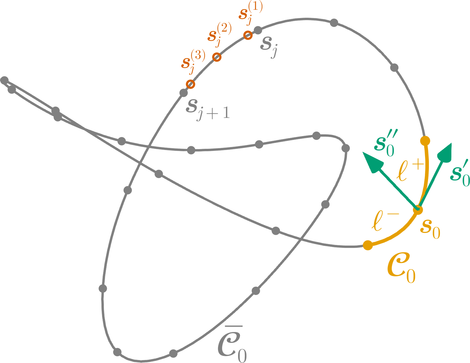
In practice, the VFM is generally used to describe length scales which are several orders of magnitude larger than . In numerical simulations, vortex filaments are discretised with a typical line resolution . Therefore, directly computing the Biot–Savart integral with a cut-off of order as described above can lead to large numerical error, especially when quadrature rules are used to estimate the integrals. For this reason, the usual approach is to split the evaluation of the Biot–Savart integral on a filament location onto local and non-local contributions [Schwarz1985], as represented in Fig. 1 for a single filament. The local contribution is estimated by analytically integrating the leading-order term of the Taylor expansion Eq. 4 on the local portion of the curve and excluding the cut-off region of length . This leads to
| (5) |
where and are the lengths of the adjacent segments composing . The local velocity is thus oriented along the local binormal direction and is proportional to the local curvature . As illustrated in Fig. 1, when filaments are discretised by connecting vortex points and is one of these points, the adjacent segments are usually defined as those linking to its neighbours.
Accounting for the local correction, the total induced velocity of a point on a vortex can be written as
| (6) |
where the prime over the integral indicates that integration is omitted on the local portion of the filament containing .
Note that neglecting the non-local contribution in Eq. 6 – thus keeping only the local part Eq. 5 – and replacing the segment lengths with a constant length scale leads to the local induction approximation (LIA), which is a widely used model of vortex motion [DaRios1906, Arms1965, Saffman1993]. This equation conserves vortex length as it disallows line stretching. Interestingly, the LIA can be mapped onto a non-linear Schrödinger equation [Hasimoto1972], a connection which is still today the subject of active research [Banica2024]. Numerically, the LIA is very convenient since it only requires local information. Filament velocities can be efficiently computed in time where is the number of vortex discretisation points. However, since it neglects all interactions between vortices, the LIA is simply not suitable for the simulation of complex configurations and in particular turbulent vortex flows [Adachi2010, Hanninen2014], where non-local effects and collective behaviour are crucial ingredients.
2.4 Energy estimation in periodic systems
The VFM described above includes no dissipation mechanisms, and kinetic energy is expected to be a conserved quantity. It is crucial to be able to accurately estimate the kinetic energy of the system, as this may allow (i) to verify the accuracy of energy conservation at the numerical level or (ii) to estimate energy decay rates when the model is extended with dissipative mechanisms.
In a periodic domain, the kinetic energy per unit mass is defined as
| (7) |
where is the main periodic cell and is its volume. In principle, this expression requires knowing the velocity field at every point in space. In the VFM this is not only impractical – as it would require many evaluations of the Biot–Savart law Eq. 3 – but is also delicate since the velocity field presents strong gradients near vortex filaments. For these reasons, in non-periodic VFM simulations [Samuels2001, Baggaley2011, Hanninen2013] the above expression is commonly replaced by111Here we express the energy is per unit density and not mass, since the domain volume (and thus the fluid mass) is infinite.
| (8) |
which only requires knowing the vortex geometry and the velocity of the vortex filaments. However, this expression assumes that the velocity and vorticity fields decay to zero at infinity [Saffman1993, Ch. 3], which is not the case in periodic domains.
An alternative expression for the kinetic energy per unit mass can be obtained from Eq. 7 using integration by parts [Saffman1993],
| (9) |
where the last equality is obtained using Eq. 2. Note that the boundary terms of the integration by parts vanish in periodic domains. In Eq. 9, we have introduced the streamfunction vector (or vector potential [Feynman2011, Saffman1993]), which is related to the velocity by , and thus to the vorticity by Poisson’s equation . In other words, the kinetic energy can be obtained from a line integral requiring knowledge of streamfunction values on vortex filaments. Interestingly, Eq. 9 also allows to interpret the tangential streamfunction, , as the linear energy density of a vortex point (up to a multiplicative constant ), and thus as the contribution of a vortex element to the total kinetic energy. Finally, note that Eq. 9 is also valid in non-periodic unbounded domains under the same assumptions leading to Eq. 8. To our knowledge, this expression has never been used before in the context of the VFM. Perhaps one of the reasons is that is a priori not available in VFM simulations, and computing it comes at an additional cost.
2.5 Obtaining the streamfunction vector
As mentioned above, the streamfunction is the solution of the Poisson equation . In three dimensions, the solution can be explicitly written as a convolution of with the Green’s function ,
| (10) |
where once again we have used Eq. 2 to express the vorticity field. Noting that , where , one can readily show that taking the curl of Eq. 10 leads to the Biot–Savart law Eq. 3.
Similarly to the velocity (Section 2.3), the streamfunction obtained via Eq. 10 diverges when evaluated on a filament location . Thus, the streamfunction integral must be desingularised by accounting for the finite radius of the vortex core. As for the velocity, we introduce a cut-off coefficient so that locations are omitted from the line integral in Eq. 10. Crucially, the cut-off coefficient need not be equal to the coefficient used for the velocity. In fact, in order for kinetic energy to be properly conserved, one must rather set , as argued analytically in Section 2.6 and verified numerically in Section 5.2.
Using the same notation as in Eq. 4, the integrand of Eq. 10 behaves close to as
| (11) |
Then, in analogy with the local velocity Eq. 5, integrating over ( segments in Fig. 1) leads to the local contribution
| (12) |
Interestingly, this term is tangent to the filament, and therefore it fully contributes to the kinetic energy Eq. 9. In the context of vortex dynamics, this local contribution is commonly referred to as vortex tension [Moore1972, Barenghi2023].
2.6 An application: vortex ring dynamics
As an illustration of the VFM and in order to justify the chosen streamfunction integration cut-off , we apply the above definitions to the classical example of an isolated circular vortex ring. Vortex rings are ubiquitous in classical and quantum fluid dynamics [Shariff1992]. In the absence of viscosity or the influence of other vortices or obstacles, they are characterised by propagating with a constant self-induced speed without changing their shape.
We consider a circular vortex ring of radius and circulation , which can be parametrised by its arc length as for . We assume periodicity effects to be negligible, i.e. , so that the influence of periodic images can be discarded. Then, under the assumption that , one can analytically compute the non-local integrals in Eqs. 6 and 13 (see e.g. [Schwarz1985] for the case of the velocity). Including the local contributions Eqs. 5 and 12, the total velocity and streamfunction on a location on the ring are
| (14) | ||||
| (15) |
We remark that the term in Eq. 15 directly comes from the choice of cut-off coefficient from the previous section, which by Eq. 9 also influences the estimated kinetic energy of the velocity field induced by the ring. The latter is explicitly given by
| (16) |
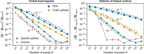
One can show that the above choice of is the only possible choice guaranteeing Hamilton’s equation [Roberts1970] to be satisfied, under the hypothesis that the vortex core size stays constant (which is imposed in the VFM). Here, is the magnitude of the hydrodynamic impulse (per unit mass) defined as
| (17) |
In the absence of non-conservative external body forces, the total impulse of a set of vortex filaments is also a conserved quantity [Saffman1993, Ch. 3]. For a circular vortex ring, the impulse is aligned with the ring velocity Eq. 14, and its magnitude is proportional to the area enclosed by the ring. One can readily differentiate both conserved quantities with respect to the ring radius ,
| (18) |
in order to verify that is indeed satisfied, using the analytical vortex ring speed in Eq. 14.
Ensuring that the adopted energy definition obeys Hamilton’s equation is critical for accurate diagnostics of energy conservation in the absence of dissipative mechanisms in the underlying model. Later in Section 5.2, we verify that using definition Eq. 12 for the local contribution to the streamfunction leads to proper energy conservation up to numerical accuracy. This appears to be the case not only for circular vortex rings, but also for complex configurations containing multiple closed vortices of arbitrary shape, and even unclosed vortices extending to infinity (as in Fig. 2, centre), in which case energy computations have been deemed impractical in the past [Baggaley2011]. Finally, note that the alternative energy expression Eq. 8 commonly used in open non-periodic systems is not consistent with Hamilton’s equation for a circular ring, as it corresponds to replacing the term in the ring energy Eq. 16 with . This suggests that Eq. 8 does not properly account for the structure of the vortex core.
2.7 Discretisation of spatial curves and line integrals
We finish this section by discussing the approach we adopt to represent vortex filaments and estimate line integrals in numerical simulations. In the context of vortex filament simulations for describing quantum fluids, filaments have been almost invariably described by a set of points in space connected by straight segments [Schwarz1985, Samuels1992, Baggaley2012f, Hanninen2013, Yui2021]. Integration of the Biot–Savart law over lines is then straightforward and can even be done analytically over each straight segment. Curve derivatives (local tangents, curvatures) are estimated on the discrete points using e.g. finite difference approximations [Baggaley2012f]. While this approach can be implemented with relative ease, it is a low-order discretisation, often requiring very small distances between discretisation points to achieve accurate results. It also presents an inconsistency between the continuity of the lines and the continuity required to estimate curvatures.
Here we take a different route and consider the filaments as smooth curves passing through a set of points, as illustrated in Fig. 1. As introduced in Section 2.1, each curve is parametrised as for some scalar parameter . The numerical degrees of freedom are the positions of discrete vortex points or nodes. Some interpolation method is then applied to evaluate vortex positions in-between nodes. The interpolation also gives direct access to curve derivatives along vortex lines, allowing to estimate local tangent and curvature vectors required for Biot–Savart computations. In the numerical experiments of Section 5 we use quintic spline interpolations which have global continuity .
In the context of the Biot–Savart problem, a second difficulty is the need to estimate integrals on vortex lines. Here we estimate line integrals using Gauss–Legendre quadratures on each segment connecting two neighbouring nodes. Concretely, if one considers a closed curve parametrised as with nodes , then an integral over such curve is approximated as
| (19) |
where is the number of quadrature points per segment (typically one chooses in simulations). Here, is a functional which may depend on curve locations as well as its derivatives. For convenience, the quadrature rule above is defined in the domain , such that are the quadrature locations, and the associated weights satisfying . Moreover, is the parameter increment associated to a single segment, with the convention that for a closed or an infinite periodic curve. As an example, the open red circles in Fig. 1 are the quadrature points associated to a single filament segment (using ).
Remark 2.1.
The use of the truncated Taylor expansions Eqs. 4 and 11 can in principle induce an error on the computation of the local velocity Eq. 5 and streamfunction Eq. 12. The error can be expected to be negligible when the vortex line discretisation is sufficiently fine. However, for computational efficiency, it may be desirable to use a coarser discretisation, in which case this source of error can become dominant. To remediate this issue, one possibility is to subdivide the local segments (Fig. 1) onto (i) a smaller central segment containing , and (ii) two outer segments respectively ending at the two nodes adjacent to . The Taylor expansions are then applied in the central segment only. In the outer segments, some quadrature rule can be used to directly evaluate the Biot–Savart and streamfunction integrals. Since these integrations are performed near the singularity at , using Gauss–Legendre quadratures with a small number of points as in Eq. 19 can result in accuracy loss, defeating the purpose of subdividing the local segments. We have found that using adaptive tanh-sinh (double exponential) quadratures [Takahasi1973, Trefethen2014] instead can provide an important gain of precision at a relatively small additional cost.
3 Fast Ewald summation for the Biot–Savart problem
In this section we adapt fast Ewald summation methods to the evaluation of velocity and streamfunction fields induced by a set of vortex filaments. This requires some adjustments since these methods generally deal with a scalar-valued source term (e.g. electrostatic charge) supported on discrete points, while here the source term (vorticity) is vector-valued and defined on spatial curves. In the context of the VFM, the basic idea of these methods is to split the line integrals in Eqs. 6 and 13 onto short- and long-range components. Concretely, including the local terms appearing in those expressions, the streamfunction and the velocity at a vortex location are decomposed as
| (20) | ||||
| (21) |
where the and superscripts denote short- and long-range components, and and are corrections to the latter which are discussed further below.
3.1 Ewald splitting
Ewald summation methods split the singular Green’s function associated to Poisson’s equation into (i) a fast decaying part accounting for short-range interactions and (ii) a slowly decaying part , which is well-behaved at and describes long-range interactions. In three dimensions, this is usually achieved via the identity ,
| (22) |
where and are respectively the error function and the complementary error function. Due to linearity, the solution to the Poisson equation is accordingly split into . Similarly, the velocity field can be decomposed as . Importantly, in Eq. 22 is the Ewald splitting parameter, which defines an inverse length scale setting the transition between short- and long-range interactions. This is a purely numerical parameter, as the physical fields and obtained by adding both contributions are in theory independent of . To facilitate the interpretation of the splitting Eq. 22, it is helpful to consider the “long-range” vorticity field defined by , which can be written as the convolution of with . In fact this is a Gaussian-filtering operation, since . In other words, is the streamfunction associated to a coarse-grained (smoothed) version of the original (singular) vorticity . Similarly, is the corresponding coarse-grained velocity field.
Taking the gradient of Eq. 22, one arrives to the corresponding splitting for the Biot–Savart kernel ,
| (23) |
with the weight functions
| (24) |
It can be verified that the long-range kernels are non-singular, behaving as and near . On the other hand, the short-range kernels asymptotically decay as and for large .
3.2 Estimation of short-range interactions
The short-range streamfunction is obtained by replacing in Eq. 10 with defined in Eq. 22, resulting in
| (25) |
where . We recall that the prime over the integral symbol denotes the omission of local vortex elements around ( segments in Fig. 1). Similarly, following the decomposition Eq. 23, the short-range velocity field is explicitly given by the modified Biot–Savart integral
| (26) |
The original integrals in Eqs. 6 and 13 are recovered by setting in the above expressions. In practice, we approximate the above line integrals using quadrature sums over discrete vortex line locations according to Eq. 19. Moreover, since the short-range kernels and decay exponentially with , one can safely define a cut-off distance beyond which short-range interactions can be neglected. The truncation errors associated to the choice of are discussed in Section 4.
3.3 Estimation of long-range interactions
Since the long-range Green’s function is non-singular, one can use a truncated Fourier series representation to indirectly solve . We start by writing the periodic vorticity field as
| (27) |
Here is the set of resolved Fourier wavenumbers in each Cartesian direction and denotes the floor operation (for simplicity, we take to be the same in all directions). We recall that represents the main periodic cell and is its volume. Since the vorticity Eq. 2 is singular and supported on spatial curves, its Fourier coefficients are then
| (28) |
where the last expression is obtained from the quadrature approximation Eq. 19. The outermost sum is over the vortex filaments of the system, each being discretised by a possibly different number of nodes . Moreover, is a shorthand for , where is the parametrisation of the -th filament, while is the derivative with respect to at that location (aligned with the local tangent vector). The triple sum in Eq. 28 can be interpreted as a sum of vector charges on locations . Note that using the same quadrature nodes for short- and long-range computations means that interpolated values of and can be shared among both components, reducing the computational cost associated to interpolations.
Now, since is the convolution of with a Gaussian kernel, its Fourier coefficients are where . Unlike , the amplitudes can be expected to decay quickly for , which justifies the truncation of the Fourier series. Moreover, solving Poisson’s equation amounts to division by in Fourier space. This ultimately allows us to express the long-range velocity in physical space as
| (29) |
Note that this requires , i.e. the mean vorticity within a periodic cell must be zero. The long-range streamfunction field can be written similarly to Eq. 29 from its Fourier coefficients .
When evaluated on a vortex location , the obtained long-range velocity and streamfunction vectors include contributions of the local segments adjacent to . However, integration over these segments must be excluded according to Eqs. 6 and 13. This issue is analogous to the spurious self-interaction electrostatic potential appearing in standard Ewald methods [Arnold2013]. In the present case, the spurious local integrals are explicitly given by
| (30) | ||||
| (31) |
where , is defined in Eq. 24, and consists of the two segments adjacent to (see Fig. 1). They can be estimated using a variant of the quadrature procedure Eq. 19, thus requiring evaluations of the integrand for each vortex location . As indicated by Eqs. 20 and 21, these two “self-interaction” terms must be subtracted from the long-range estimations to avoid an unphysical dependence of the results on the Ewald parameter .
In the present context, the main difficulty of fast Ewald summation methods is the estimation of the Fourier coefficients of the vorticity field Eq. 28 and the evaluation of the resulting coarse-grained fields on arbitrary physical locations Eq. 29. While these two operations can in principle be directly evaluated according to their definitions, this is extremely inefficient, and fast approximations are required in practical applications. In fact, there are many variants of fast Ewald summation (so-called PM, PME, SPME, PNFFT, …) which mainly differ on how these operations are performed [Deserno1998, Arnold2013]. What they all have in common is that they introduce a regular 3D grid, which enables the acceleration of these operations using FFTs. First, point charges are spread onto the grid by some smoothing (spreading) operation, and Eq. 28 is then estimated using FFTs. Then, the Laplacian is generally inverted in Fourier space using some kind of modified Green’s function [Hockney1988, Deserno1998, Ballenegger2008] which accounts for errors introduced by the spreading and interpolation operations. Finally, Eq. 29 is estimated using backwards FFTs followed by an interpolation from the grid to the target locations. An important realisation [Hedman2006, Arnold2013, Pippig2013] is that all of these operations can be conveniently and efficiently performed using the non-uniform fast Fourier transform (NUFFT) algorithm [Dutt1993]. In fact, the sums in Eq. 28 and Eq. 29 respectively correspond to type-1 (non-uniform to uniform) and type-2 (uniform to non-uniform) NUFFTs [Greengard2004]. From a practical standpoint, this eases the development of Ewald methods and allows one to rely on recent theoretical developments and on existent fast and accurate NUFFT implementations. When relying on the NUFFT, the accuracy of long-range computations is then controlled by the NUFFT accuracy and the truncation wavenumber . These two sources of error are respectively discussed in Appendix B and Section 4.
4 Truncation error estimates
We now provide estimates of the root-mean-square errors associated to the short- and long-range cut-offs and . Similar estimates have already been provided for the electrostatic problem [Kolafa1992, Deserno1998a], but these do not directly apply to the VFM since (i) the quantities of interest are not the same, and (ii) the singular sources in the present case are spatial curves and not points. We also show that the effect of the parameters , and can be reduced to a unique non-dimensional coefficient which can be tuned to control the method accuracy, thus greatly simplifying the parameter selection procedure.
The derivation of the error estimates is detailed in Appendix C. In summary, the estimates make the simplifying assumptions that (i) vortex filaments are homogeneously distributed in the spatial domain, (ii) the relative orientation of two vortex elements at a distance is completely decorrelated, and (iii) is much larger than the typical curvature of the vortices. Introducing the non-dimensional cut-off coefficients and , we show that both short- and long-range errors decay exponentially with the square of these respective coefficients, which justifies reducing them into a unique coefficient . This finally leads to the truncation error estimates
| (32) | ||||
| (33) |
where the short- and long-range contributions to the errors correspond to the first and second terms within each square bracket. The accuracy of the method is thus mainly driven by a unique non-dimensional parameter . This sets both physical- and Fourier-space cut-offs and for a given value of the inverse splitting distance , which is left as a free parameter that can be adjusted to optimise performance (Section 5.3).
5 Numerical experiments
We now perform different numerical experiments to evaluate the accuracy, conservation properties and computational complexity of the proposed FFT-based method. All computations are performed in double precision arithmetic and the methods are implemented in the Julia programming language [Bezanson2017]. In all numerical tests below, the domain is periodic with period in all directions. The vortex core size and the vorticity profile parameter – both appearing in the locally induced velocity Eq. 5 – are respectively set to and , and the vortex circulation is set to . Vortex lines are represented as smooth curves using quintic splines (see Appendix A for details), which allows to estimate derivatives and evaluate quantities in-between discretisation points. Moreover, line integrals are estimated using quadrature points per vortex segment (see Section 2.7).
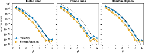
5.1 Accuracy
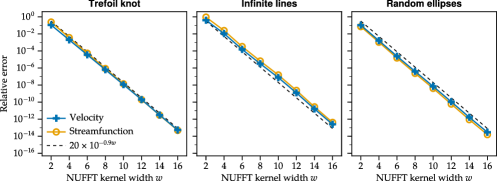
To numerically assess the accuracy of the proposed method, we consider three different test cases of varying complexity. The test cases are detailed below and illustrated in Fig. 2.

1. Trefoil knot
The trefoil knot consists in a single knotted curve (Fig. 2, left), interacting with itself and its periodic images. The trefoil knot curve is parametrically defined by
| (34) |
where determines the size of the trefoil knot. We take so that periodicity effects are non-negligible. The curve is discretised by evaluating Eq. 34 on equally spaced values of .
2. Infinite lines
This test case consists of a set of straight infinitely extended lines inducing a three-dimensional velocity field. Each periodic cell is crossed by three pairs of lines aligned positively and negatively with each Cartesian direction (Fig. 2, centre). The filament orientations are such that the velocity induced on each line is non-zero and positively aligned with the line (). Since the lines have zero curvature, the velocity induced by a line on itself is zero, and therefore the velocity of a vortex point is completely due to non-local interactions. Therefore, this test case emphasises the accuracy of long-range computations. We discretise each filament with independent nodes (for ).
3. Random ellipses
The third test case is closer to a disordered configuration relevant to turbulent vortex flows. It consists of 40 ellipses which are randomly positioned and oriented within the spatial domain (Fig. 2, right). The size and aspect ratio of each ellipse is also random. Concretely, the minor and major radii are random values uniformly and independently distributed in . We discretise each ellipse with nodes (for ).
Empirical relative errors
To numerically quantify the truncation errors in each test case, we start by computing a reference solution with very high accuracy. Concretely, we set the cut-off coefficient to and compute NUFFTs with a nominal relative tolerance . Here, the reference solution corresponds to a set of velocity and streamfunction values, ψ_i
References
-
[1]
, on each discrete filament
node .
We then compare this reference solution with the results and
obtained by varying .
The splitting parameter is set to
in all numerical experiments.
Accuracy estimates are obtained by evaluating the relative
errors
where the norm of a vector field evaluated at discrete locations is defined by . Here denotes the vector magnitude.(35) - [6]
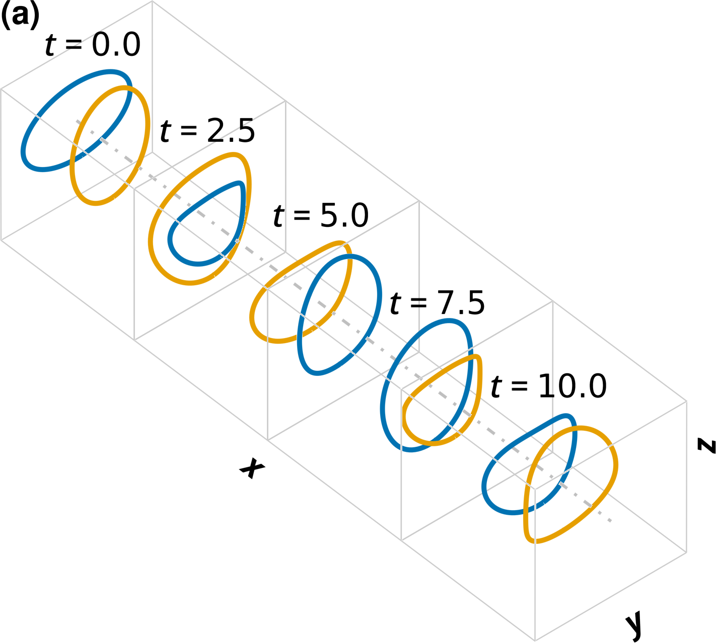
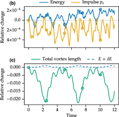
5.2 Timestepping and conservation properties
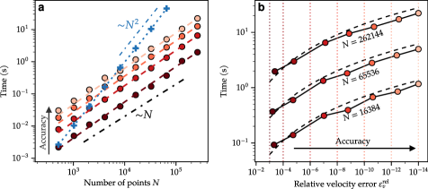
5.3 Performance
| (36) |
| () | (%) | |||||
|---|---|---|---|---|---|---|
6 Conclusions
Acknowledgments
Appendix A Discretisation of spatial curves
A.1 Curve discretisation schemes
A.1.1 Finite difference approximations
A.1.2 Spline interpolation
| (37) |
A.1.3 Fourier series representation
| (38) |
A.2 Accuracy of different discretisation methods
| (39) |
Appendix B NUFFT details and influence on Biot–Savart accuracy
| (40) |
Appendix C Derivation of truncation error estimates
C.1 Short-range errors
| (41) |
| (42) |
| (43) |
| (44) |
| (45) |
C.2 Long-range errors
| (46) |
| (47) |
| (48) |
| (49) |
| (50) |
| (51) |
| (52) |