Fractonic solids

Abstract

Fractons are exotic quasiparticles whose mobility in space is restricted by symmetries. In potential real-world realisations, fractons are likely lodged to a physical material rather than absolute space. Motivated by this, we propose and explore a new symmetry principle that restricts the motion of fractons relative to a physical solid. Unlike models with restricted mobility in absolute space, these fractonic solids admit gauge-invariant momentum density, are compatible with boost symmetry, and can consistently be coupled to gravity. We also propose a holographic model for fractonic solids.

Given a physical model with local degrees of freedom and local interactions, we typically expect its low-energy course-grained description to be reliably captured by a local effective field theory. However, in recent years, various lattice models of interest in condensed matter and high energy physics have emerged [1, 2, 3, 4], whose low-energy descriptions feature exotic characteristics atypical of a well-posed effective field theory. The most striking characteristic of these models are local quasi-particle excitations, called fractons, that cannot move freely in space despite translational invariance; see reviews [5, 6].

The bizarre nature of fractons in many of these models can be ascribed to emergent subsystem symmetries that act independently on different parts of the system [7, 8, 9, 10]. It is helpful to model these in terms of a series of multipole symmetries [11, 12]. Consider, e.g., a complex scalar field $\Psi$ invariant under the U(1) transformations

$$\Psi\to{\rm e}^{i\Lambda_{\text{ss}}(\vec{x})}\,\Psi={\rm e}^{i\Lambda+i\Lambda_{i}x^{i}+\frac{i}{2}\Lambda_{ij}x^{i}x^{j}\ldots}\,\Psi.$$ (1)

The monopole symmetry $\Lambda$ imposes charge conservation; the dipole symmetry $\Lambda_{i}$ restricts the motion of free charges and only allows them to move in neutral bound states with fixed dipole moment; and similarly for higher moments. The associated symmetry algebra is characterised by the non-trivial commutation relations [12]

$$[\mathrm{P}_{i},\mathrm{Q}^{j}]=i\delta_{i}^{j}\mathrm{Q},\quad[\mathrm{P}_{i},\mathrm{Q}^{jk}]=2i\delta_{i}^{(j}\mathrm{Q}^{k)},\quad\ldots,$$ (2)

between the momenta $\mathrm{P}_{i}$ and the multipole generators $\mathrm{Q},\mathrm{Q}_{i},\mathrm{Q}_{ij},\ldots$. This implies, for instance, that translations do not commute with dipole transformations when acting on charged states.

A byproduct of restricted spatial mobility is that multipole symmetries do not play well with spacetime symmetries. They are outright incompatible with boost transformations and thus cannot be realised in relativistic or Galilean systems. In particular, multipole-invariant field theories cannot consistently be coupled to general relativistic gravitational spacetimes [13, 14]. They can be made compatible with spacetime translations, but require exotic boost-agnostic spacetime geometries to couple to the associated energy-momentum currents [15, 14, 16]. Moreover, momentum is not invariant under multipole transformations in these theories and leads to peculiarities such as no low-energy phases with spontaneously unbroken multipole symmetries [17, 18] and lack stable hydrodynamic states with nonzero velocity [19, 20, 21, 22, 23, 24].

While fractons remain largely a theoretical curiosity, various condensed matter systems are expected to realise fractonic excitations at low energies. Examples include topological defects in crystals and superfluids [25, 26, 27, 28, 29], majorana islands [30], plaquette paramagnets [31], hole-doped antiferromagnets [32], and tilted optical lattices [33]. In such physical realisations, one expects that fractons are embedded on a physical material but they may move in absolute space when the material itself is strained or distorted. Accounting for the dynamics of the underlying material may also help ease tensions between multipole and spacetime symmetries. As a first step in this direction, the goal of this letter is to investigate effective field theories for fractons whose motion is restricted with respect to a dynamical crystal.

We cannot naively append elastic crystal dynamics to the multipole symmetries (2). This would correspond to an unnatural scenario where fractons stay lodged in absolute space while the crystal is distorted. We need to instead modify the multipole symmetry itself to make it aware of the crystalline structure. A crystal in $d$ spatial dimensions is described by a collection of crystal fields $\phi^{I=1,\ldots,d}$ representing the Eulerian coordinates of the underlying lattice sites as a function of time and space $(x^{\mu})=(t,x^{i})$ [34, 35, 36, 37]. To impose mobility restrictions on the crystal, we adapt the multipole transformations in (1) using $\phi^{I}$ as

$$\Psi\to{\rm e}^{i\Lambda_{\text{ss}}(\phi^{I}(x))}\,\Psi={\rm e}^{i\Lambda+i\Lambda_{I}\phi^{I}(x)+\frac{i}{2}\Lambda_{IJ}\phi^{I}(x)\phi^{J}(x)+\ldots}\,\Psi,$$ (3)

which reduces to (1) when the crystal is fixed to a homogeneous state $\phi^{I}=\delta^{I}_{i}x^{i}$. However, beyond this simple state, the crystal-multipole symmetries (3) depend non-linearly on the crystal configuration and thus qualitatively differ from the spatial-multipole symmetries (1). See figure 1. The spatial-momenta $\mathrm{P}_{i}$ in the symmetry algebra (2) are appropriately replaced by the crystal momenta $\mathrm{P}_{I}$ that generate crystal translations $\phi^{I}\to\phi^{I}+a^{I}$, i.e.

$$[\mathrm{P}_{I},\mathrm{Q}^{J}]=i\delta_{I}^{J}\mathrm{Q},\quad[\mathrm{P}_{I},\mathrm{Q}^{JK}]=2i\delta_{I}^{(J}\mathrm{Q}^{K)},\quad\ldots.$$ (4)

Since the crystal-multipole transformations (3) only talk to the spacetime coordinates via the crystal fields, they get along better with spacetime symmetries. In particular, field theories with crystal-multipole symmetries are compatible with boosts, can be realised in relativistic or Galilean systems, can be coupled to dynamical gravity, admit translationally-invariant phases with spontaneously unbroken crystal-multipole symmetries, and allow stable states with nonzero velocity. We will investigate all these aspects in detail in this letter, specialising to relativistic systems with crystal-dipole symmetry.

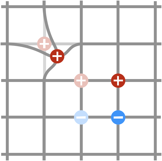
Figure 1: Crystal-dipole symmetry. Isolated free charges cannot move on the crystal, but can move in space when the crystal is distorted. Neutral bound states can move freely on the crystal while keeping their crystal-dipole moment fixed.

Field theory with crystal-dipole symmetry

—A crystal naturally defines the spacelike frame fields $e^{I}_{\mu}=\partial_{\mu}\phi^{I}$ and the timelike frame velocity $v^{\mu}$ s.t. $v^{\mu}e^{I}_{\mu}=0$, $v^{\mu}v_{\mu}=-1$. Raising/lowering of spacetime and crystal indices is performed using the relativistic spacetime metric $g_{\mu\nu}$ and the crystal metric $h^{IJ}=e^{I\mu}e^{J}_{\mu}$ respectively. Using this dynamical segregation between time and space, and drawing motivation from spatial-dipole-invariant field theories in [38], we can engineer a crystal-dipole-invariant Lagrangian for a relativistic complex scalar field $\Psi$, e.g.

$${\cal L}_{\Psi}=|\mathrm{D}_{v}\Psi|^{2}-\lambda\,|\mathrm{D}_{IJ}(\Psi,\Psi)|^{2}-V(|\Psi|^{2}),$$ (5)

for some parameter $\lambda$ and potential $V(|\Psi|^{2})$, where the derivative operators are defined as

$$\mathrm{D}_{IJ}(\Psi,\Psi) =\Psi\mathrm{D}_{(I}\mathrm{D}_{J)}\Psi-\mathrm{D}_{I}\Psi\mathrm{D}_{J}\Psi,$$

$$\mathrm{D}_{v} =v^{\mu}\nabla_{\mu},\qquad\mathrm{D}_{I}=e^{\mu}_{I}\nabla_{\mu},$$ (6)

and $\nabla_{\mu}$ is the spacetime covariant derivative. One may explicitly check that the theory is invariant under global symmetries: crystal-translations, crystal-rotations, monopole and crystal-dipole transformations, as well as spacetime Poincaré transformations. In particular, a quadratic spatial derivative term $|\mathrm{D}_{I}\Psi|^{2}$ is forbidden by crystal-dipole symmetry. For a fixed homogeneous crystal, $\phi^{I}=\delta^{I}_{i}x^{i}$, this theory reduces to the model of [38] with spatial-dipole symmetry and explicitly broken Lorentz-invariance.

To account for crystal dynamics, the Lagrangian also contain an elastic part $\mathcal{L}_{\text{el}}(\kappa_{IJ})$ comprising the crystal strain tensor $\kappa_{IJ}=\frac{1}{2}(h_{IJ}-\delta_{IJ})$ that measures distortions away from a reference configuration. See [39, 35] for more details on effective field theory of relativistic crystals.

Gauging fields and conserved currents

—We can gauge the monopole and crystal-dipole symmetries by introducing gauge fields $A_{\mu}$, $A_{I\mu}$ that transform as

$$A_{\mu} \to A_{\mu}+\partial_{\mu}\Lambda-a^{I}A_{I\mu},\quad A_{I\mu}\to A_{I\mu}+\partial_{\mu}\Lambda_{I}.$$ (7)

The shift of $A_{\mu}$ under crystal translations $a^{I}$ is required by the crystal-dipole symmetry algebra in (4). More details on the gauging procedure can be found in the appendix. The gauge-covariant derivative of $\Psi$ is defined as $\mathrm{D}_{\mu}\Psi=\partial_{\mu}\Psi-i\left(A_{\mu}+\phi^{I}A_{I\mu}\right)\Psi$, extending the derivative operators in (6) to

$$\mathrm{D}_{IJ}(\Psi,\Psi) =\Psi\mathrm{D}_{(I}\mathrm{D}_{J)}\Psi-\mathrm{D}_{I}\Psi\mathrm{D}_{J}\Psi-ie^{\mu}_{(I}A_{J)\mu}\Psi^{2},$$

$$\mathrm{D}_{v} =v^{\mu}\mathrm{D}_{\mu},\qquad\mathrm{D}_{I}=e^{\mu}_{I}\mathrm{D}_{\mu}.$$ (8)

With these definitions, the complex scalar field theory in (5) becomes invariant under local monopole and crystal-dipole transformations.

Varying the effective action $S=\int_{d+1}\mathcal{L}$ of the theory with respect to the background metric and gauge fields, we can read off the respective conserved currents: symmetric energy-momentum tensor $T^{\mu\nu}$, charge monopole current $J^{\mu}$, and crystal-dipole current $J^{\mu I}$, i.e.

$$\delta S=\int_{d+1}\frac{1}{2}T^{\mu\nu}\delta g_{\mu\nu}+J^{\mu}\delta A_{\mu}+(J^{\mu I}+J^{\mu}\phi^{I})\delta A_{I\mu},$$ (9)

where $\int_{d+1}$ is shorthand for $\int\mathrm{d}t\mathrm{d}^{d}\vec{x}\,\sqrt{-\det g}$. We have isolated the “free” contribution $J^{\mu}\phi^{I}$ from the “internal” dipole current $J^{\mu I}$ to make it invariant under crystal-translations. The conservation equations are given as

$$\nabla_{\mu}T^{\mu\nu}=\tilde{F}^{\nu\rho}J_{\rho}+F_{I}^{\nu\rho}J^{I}_{\rho},$$

$$\nabla_{\mu}J^{\mu}=0,\qquad\nabla_{\mu}J^{\mu I}=-e^{I}_{\nu}J^{\nu},$$ (10)

where we have defined the monopole and crystal-dipole gauge field strengths $F_{\mu\nu}=2\partial_{[\mu}A_{\nu]}$, $F_{I\mu\nu}=2\partial_{[\mu}A_{I\nu]}$, together with the combination $\tilde{F}_{\mu\nu}=F_{\mu\nu}+\phi^{I}F_{I\mu\nu}$ that is invariant under crystal-translations. The third conservation equation is the crystalline incarnation of the dipole Ward identity, which relates the divergence of the internal crystal-dipole current to the monopole flux along the crystal. The total crystal-dipole moment

$$\int\mathrm{d}^{d}\vec{x}\sqrt{-g}\left(J^{0}\phi^{I}+J^{0I}\right),$$ (11)

is conserved, together with the total energy-momentum and charge. For the complex scalar field theory in (5), the conserved currents $J^{\mu}$ and $J^{\mu I}$ are given as

$$J^{\mu} =-iv^{\mu}\Psi\mathrm{D}_{v}\Psi^{*}-i\lambda e^{\mu}_{I}\,\partial_{\nu}\Big{(}e^{\nu}_{J}\mathrm{D}^{\dagger IJ}(\Psi,\Psi)\Psi^{2}\Big{)}+\text{c.c.},$$

$$J^{\mu I} =i\lambda e^{\mu}_{J}\mathrm{D}^{\dagger IJ}(\Psi,\Psi)\Psi^{2}+\text{c.c.},$$ (12)

where “c.c.” denotes the complex conjugate. The expression for $T^{\mu\nu}$ is given in the appendix.

Crystal-dipole gauge theory

—We can give dynamics to the monopole and crystal-dipole gauge fields by introducing new kinetic terms in the Lagrangian, e.g.

$${\cal L}_{\text{gauge}} =-\frac{1}{4g_{0}}\tilde{F}_{\mu\nu}\tilde{F}^{\mu\nu}-\frac{1}{4g_{1}}F_{I\mu\nu}F^{I\mu\nu}.$$ (13)

More general terms may be included by projecting the field strengths along $v^{\mu}$ and $e_{\mu}^{I}$. The respective Maxwell-type equations and Bianchi identities are given as

$$\nabla_{\nu}\tilde{F}^{\mu\nu} =g_{0}J^{\mu}, \nabla_{\nu}F^{I\mu\nu} =g_{1}J^{I\mu}-\frac{g_{1}}{g_{0}}e^{I}_{\nu}\tilde{F}^{\mu\nu},$$

$$\nabla_{[\mu}\tilde{F}_{\nu\rho]} =e^{I}_{[\mu}F_{I\nu\rho]},\qquad \nabla_{[\mu}F_{I\nu\rho]} =0.$$ (14)

These may be understood as a relativistic extension of the symmetry-tensor gauge theory studied in [38], embedded on a dynamical crystal. To wit, the field strength components $\tilde{F}_{\mu\nu}$, $F_{[ij]t}$, $F_{[ijk]}$, where $F_{\mu\nu\rho}=e_{I}^{\mu}F_{I\nu\rho}$, are gapped due to the second and third equations in (Crystal-dipole gauge theory). Taking $d=3$, the remaining gapless components are contained in the tensor analogues of electric and magnetic fields

$$E_{ij}=F_{(ij)t}+\partial_{(i}\tilde{F}_{j)t},\quad B_{i}^{\leavevmode\nobreak\ j}=\frac{1}{2}\epsilon^{jkl}(F_{ikl}-\partial_{k}\tilde{F}_{li}),$$ (15)

satisfying $E_{[ij]},B_{i}^{\leavevmode\nobreak\ i}=0$, which behave analogous to the symmetric-tensor gauge theory at the linearised level. However, the dynamics differs significantly at the non-linear level due to interactions with the crystal and depends on the explicit form of the Lagrangian (13).

Spontaneous symmetry breaking

—As a phase of matter, crystals or solids spontaneously break spatial translation symmetry, with $\phi^{I}$ identified as the respective Goldstones. Analogous to the supersolid phase that further spontaneously breaks the U(1) particle conservation symmetry [40], we may consider multipole supersolids with spontaneously broken crystal-multipole symmetries. Following [41, 18], there are two distinct possibilities for systems with crystal-dipole symmetry: a p-wave phase with $\langle\Psi\rangle=0$, $\langle i\Psi^{\dagger}\mathrm{D}_{I}\Psi\rangle\neq 0$ where the crystal-dipole symmetry is spontaneously broken but the monopole remains unbroken, and an s-wave phase with $\langle\Psi\rangle\neq 0$ where both are spontaneously broken.

The p-wave phase is characterised by a vector Goldstone field $\varphi_{I}$, transforming as $\varphi_{I}\to\varphi_{I}-\Lambda_{I}$. Defining the crystal-dipole superfluid velocity $\xi_{I\mu}=\partial_{\mu}\varphi_{I}+A_{I\mu}$, we may write down a simple effective Lagrangian

$${\cal L}_{\text{p-wave}} =\frac{1}{2}\chi_{d}(v^{\mu}\xi_{I\mu})^{2}+V({\textstyle\xi_{I}^{\leavevmode\nobreak\ J}}),$$ (16)

where the potential $V$ depends on $\xi_{IJ}=\xi_{I\mu}e^{J\mu}$. In contrast, the s-wave phase is characterised by a scalar Goldstone field $\varphi$, transforming as $\varphi\to\varphi-\Lambda-\Lambda_{I}\phi^{I}$. The second term in the transformation is necessitated by the symmetry algebra (4). As a consequence, the superfluid velocity $\xi_{\mu}=\partial_{\mu}\varphi+A_{\mu}+\phi^{I}A_{I\mu}$ is invariant under the monopole symmetry but not the crystal-dipole symmetry. In fact, $\xi_{I}\equiv e_{I}^{\mu}\xi_{\mu}$ transforms exactly like the vector Goldstone $\varphi_{I}$, justifying that the crystal-dipole symmetry is automatically spontaneously broken, and we may use it to define $\xi_{I\mu}=\partial_{\mu}\xi_{I}+A_{I\mu}$. Using these ingredients, we may construct the effective Lagrangian, e.g.

$${\cal L}_{\text{s-wave}} =\frac{1}{2}\chi\,(v^{\mu}\xi_{\mu})^{2}+\frac{1}{2}\chi_{d}(v^{\mu}\xi_{I\mu})^{2}+V({\textstyle\xi_{I}^{\leavevmode\nobreak\ J}}),$$ (17)

which is similar in form to eq. 16, but with a new kinetic term $\sim(v^{\mu}\xi_{\mu})^{2}$ for the scalar Goldstone.

Hydrodynamics

—Imposing mobility restrictions on a dynamical crystal instead of absolute space has qualitative impact on the low-energy thermal phases. The dynamics of a system at finite temperature is described by the framework of hydrodynamics . Therein, one specifies the constitutive relations for the conserved currents $T^{\mu\nu}$, $J^{\mu}$, $J^{\mu I}$ in terms of the hydrodynamic variables: fluid velocity $u^{\mu}$ (s.t. $u^{\mu}u_{\mu}=-1$), temperature $T$, chemical potential $\mu$, crystal-dipole chemical potential $\mu_{I}$, and the crystal fields $\phi^{I}$. To wit, consider

$$T^{\mu\nu} =(\epsilon+p)u^{\mu}u^{\nu}+p\,g^{\mu\nu}-r^{IJ}e^{\mu}_{I}e^{\nu}_{J}$$

$$\qquad-2\eta\Delta^{\mu\rho}\Delta^{\nu\sigma}\nabla_{(\rho}u_{\sigma)}-\left(\zeta-{\textstyle\frac{2}{d}}\eta\right)\Delta^{\mu\nu}\nabla_{\lambda}u^{\lambda},$$

$$J^{\mu} =n\,u^{\mu}-\sigma\Delta^{\mu\nu}\left(T\partial_{\nu}\frac{\mu}{T}-\mu_{I}e^{I}_{\nu}-\tilde{F}_{\nu\rho}u^{\rho}\right),$$

$$J^{\mu I} =n^{I}u^{\mu}-\sigma_{\rm d}\Delta^{\mu\nu}h^{IJ}\left(T\partial_{\nu}\frac{\mu_{J}}{T}-F_{J\nu\rho}u^{\rho}\right).$$ (18)

The energy density $\epsilon$, pressure $p$, entropy density $s$, charge density $n$, crystal-dipole density $n^{I}$, and elastic stress $r_{IJ}$ obey the thermodynamic relations

$$\mathrm{d}p =s\,\mathrm{d}T+n\,\mathrm{d}\mu+n^{I}\mathrm{d}\mu_{I}+\frac{1}{2}r_{IJ}\mathrm{d}h^{IJ},$$

$$\epsilon =Ts+\mu n+\mu_{I}n^{I}-p,$$ (19)

We have also introduced the dissipative viscosities $\eta$, $\zeta$ and conductivities $\sigma$, $\sigma_{\rm d}$. The conservation equations (10) govern the dynamics of $u^{\mu}$, $T$, $\mu$, $\mu_{I}$, while that of $\phi^{I}$ is governed by the Josephson equation

$$K_{I} \equiv-\nabla_{\mu}\!\left(r_{IJ}e^{J\mu}\right)+n\mu_{I}-\sigma_{\phi}u^{\mu}e_{I\mu}=0,$$ (20)

with the crystal diffusion parameter $\sigma_{\phi}$. The form of hydrodynamic equations is dictated by the local second law of thermodynamics; see the appendix for more details. However, we have only included a selection of transport coefficients here for simplicity.

Let us look at the spectrum of linearised hydrodynamic fluctuations around the equilibrium solution: $u^{\mu}=\delta^{\mu}_{t}$, $T=T_{0}$, $\mu=\mu_{0}$, $\mu_{I}=0$, and $\phi^{I}=\delta^{I}_{i}x^{i}$, in the absence of background sources. For an ordinary crystal, the spectrum contains longitudinal sound modes $\omega\sim\pm k$, transverse phonon modes $\omega\sim\pm k$, and two coupled charge and crystal diffusion modes $\omega\sim-ik^{2}$. However, due to crystal-dipole symmetry, the charge diffusion mode decouples and becomes subdiffusive

$$\omega=-ik^{4}\frac{\sigma_{\rm d}}{\partial n/\partial\mu+n^{2}/(B+2\frac{d-1}{d}G)},$$ (21)

where $B$, $G$ are the elastic moduli parametrising the elastic stress $r_{IJ}=2G\kappa_{IJ}+(B-\frac{2}{d}G)h_{IJ}\operatorname{tr}\kappa$. Such subdiffusive modes are characteristic of fracton hydrodynamics. Importantly, here subdiffusion arises without spontaneously broken crystal-dipole symmetry, whereas there are no analogous momentum-conserving phases without spontaneously broken spatial-dipole symmetry [17, 18].

The constitutive relations for p-wave and s-wave phases additionally depend on $f^{I}_{\leavevmode\nobreak\ J}=\partial p/\partial\xi_{I}^{\leavevmode\nobreak\ J}$. Following through the second law analysis, we find that the crystal-dipole current in the p-wave phase gets a superflow contribution $J^{\mu I}\sim f^{IJ}e_{J}^{\mu}$ while the monopole current remains the same. Whereas, in the s-wave phase, the monopole current also gets a superflow contribution $J^{\mu}\sim-\nabla_{\nu}\!\left(f^{IJ}e_{J}^{\nu}\right)e_{I}^{\mu}$. We also find Josephson equations for the respective Goldstones, $u^{\mu}\xi_{I\mu}\sim\mu_{I}$ and $v^{\mu}\xi_{\mu}\sim\mu/(u\cdot v)$. The details of the constitutive relations appear in the appendix. The fluid sound and crystal phonon/diffusion modes remain unaffected in these phases. Whereas, the subdiffusive mode (21) is affected qualitatively similarly to spatial-dipole superfluids without energy-momentum conservation [41]. In the s-wave phase, the subdiffusive mode gets replaced by a magnon-like propagating mode $\omega\sim\pm k^{2}$. In the p-wave phase, however, it is replaced by a transverse diffusion mode $\omega=-ik^{2}$ and two longitudinal diffusion modes $\omega\sim-ik^{2}$ or magnon-like modes $\omega\sim\pm k^{2}$ depending on the parameters of the model. The details are included in a supplementary Mathematica notebook.

This spectrum is quite different from the analogous momentum-conserving phases with spatial-dipole symmetry. For instance, the fluid sound mode in the spatial-dipole p-wave phase shows magnon-like dispersion. Furthermore, the spatial-dipole p-wave phase does not admit any states with nonzero fluid velocity, while such states are unstable in the spatial-dipole s-wave phase [19, 21, 22, 23, 24]. One the other hand, finite velocity states are automatically stable in our models on account of boost symmetry .

Fixed crystals

—One may consider physical setups where fractons are embedded on a rigid crystal and thus the elastic dynamics of $\phi^{I}$ may be ignored. In this case, $\phi^{I}$ become fixed background fields and the crystal-multipole symmetries effectively reduce to the previously explored spatial-multipole symmetries. Any boost symmetry of the theory also gets explicitly broken by the fixed reference frame $v^{\mu}$ provided by the crystal. We can combine the fixed $\phi^{I}$ with the background metric, connection, and crystal-multipole gauge fields to derive the Aristotelian background sources suitable for coupling to spatial-multipole-invariant field theories [14, 16]. A detailed comparison is carried out in the appendix. In fact, if we assume that $\phi^{I}$ only appears in the theory implicitly via the Aristotelian sources, we immediately arrive at momentum-conserving field theories invariant under spatial-multipole symmetries.

Generically, however, we expect a fixed background crystal to act as a momentum sink and endow relaxational dynamics to momentum fluctuations [36]. To wit, if we allow for arbitrary dependence on $\phi^{I}$, the operator $K_{I}$ in eq. 20 is not set to zero for a non-dynamical crystal and instead shows up as a source in the energy-momentum conservation as $K_{I}e^{I\nu}$. Expanding around a fixed background $\phi^{I}=\delta^{I}_{i}x^{i}$, this contribution relaxes velocity/momentum fluctuations with a characteristic rate $\sigma_{\phi}/(\epsilon+p)$. In other words, the only low-energy variables in such systems are energy, charge with relevant multipole symmetries, and the relevant Goldstone fields for spontaneous symmetry breaking. Interestingly, without a momentum component, one may consistently consider states without spontaneous symmetry breaking [17, 41] and the question of nonzero velocity states does not arise in the first place.

Fracton holography

—Fractons have thus far been theoretically realised in a variety of lattice spin models with exotic interactions. However, such models typically feature UV/IR mixing and it is unclear whether there exists an unambiguous renormalisation group prescription that may be used for a bottom-up derivation of their low-energy effective descriptions; see [44]. It will be interesting to investigate whether the crystal-multipole-invariant theories discussed here fare any better. That said, since crystal-multipole symmetries can be made consistent with relativity, and can be consistently coupled to gravity, they open up an alternate possibility of using holography or the AdS/CFT correspondence for modelling fractons.

The simplest such holographic model can be obtained by extending the holographic model for charged viscoelasticity studied in [45, 35] to include crystal-dipole gauge fields in the bulk, i.e.

$$\frac{1}{2}\int_{d+2}R-2\Lambda-\frac{1}{4}\tilde{\mathcal{F}}_{{\textsl{{m}}}{\textsl{{n}}}}\tilde{\mathcal{F}}^{{\textsl{{m}}}{\textsl{{n}}}}-\frac{1}{4}\mathcal{F}_{I{\textsl{{m}}}{\textsl{{n}}}}\mathcal{F}^{I{\textsl{{m}}}{\textsl{{n}}}}-V(X).$$ (22)

Here $R-2\Lambda$ is the familiar Einstein-Hilbert gravitational term for the bulk metric $g_{{\textsl{{m}}}{\textsl{{n}}}}$, with ${\textsl{{m}}},{\textsl{{n}}},\ldots$ denoting the $(d+2)$-dimensional bulk indices, and negative cosmological constant $\Lambda=-\frac{1}{2}d(d+1)$. The potential $V$ depends on $X=\frac{1}{2}\delta_{IJ}H^{IJ}$, where $H^{IJ}=g^{{\textsl{{m}}}{\textsl{{n}}}}\partial_{\textsl{{m}}}\Phi^{I}\partial_{\textsl{{n}}}\Phi^{J}$ contains the bulk crystal fields $\Phi^{I}$. Lastly, $\tilde{\mathcal{F}}_{{\textsl{{m}}}{\textsl{{n}}}}$, $\mathcal{F}_{I{\textsl{{m}}}{\textsl{{n}}}}$ denote the field strengths associated with dynamical monopole and crystal-dipole gauge fields $\mathcal{A}_{\textsl{{m}}}$, $\mathcal{A}_{I{\textsl{{m}}}}$ in the bulk. The charged black brane solution in [45, 35] still solves this model with a trivial profile for the dipole gauge field $\mathcal{A}_{I{\textsl{{m}}}}=0$. In the dual boundary theory, this corresponds to an equilibrium state with zero crystal-dipole chemical potential. However, the dynamics of this model would differ significantly from that of [45, 35] due to fluctuations of $\mathcal{A}_{I{\textsl{{m}}}}$. In particular, we expect to find a subdiffusive mode $\omega\sim-ik^{4}$ in the spectrum of quasinormal modes of the black brane.

Interestingly, the holographic model (22) may describe fractons on a dynamical or fixed background crystal depending on the boundary conditions imposed on the bulk crystal fields $\Phi^{I}$. However, for the fixed crystal boundary conditions, the momentum fluctuations in the boundary theory are relaxed [45], so we expect to find momentum-non-conserving fracton hydrodynamic theories analogous to [19] with spontaneously unbroken monopole and spatial-dipole symmetries, but with an added conserved energy component. The holographic models for p-wave and s-wave phases, for both dynamical or fixed background crystals, may be obtained by including appropriately charged matter in the bulk along the lines of [46, 47].

Outlook

—In this letter, we have developed fractonic field theories where charged excitations have restricted mobility within a physical crystal, but are permitted to move in absolute space along with the crystal. This is realised through a new class of crystal-multipole symmetries that require the conservation of relevant multipole moments relative to the crystal. We discussed how to gauge these symmetries, giving rise to gapless crystal-multipole gauge theories that are the analogues of tensor gauge theories that arise in the context of spatial-multipole symmetries. We also discussed spontaneously broken crystal-multipole symmetries, giving rise to exotic supersolid phases with mobility restrictions.

The most distinctive aspect of crystal-multipole symmetries is that, unlike their spatial-multipole counterparts, they feature gauge-invariant spatial momenta and thus are compatible with boost symmetries. We exploited this to construct, for the first time, relativistic field theories with fractonic excitations that can be consistently coupled to generic curved gravitational backgrounds. As a result of boost-invariance, these theories also allow for stable hydrodynamic states with nonzero fluid velocity that are forbidden by spatial-multipole symmetries. This has also allowed us to propose a new class of holographic models for studying fractons in the context of AdS/CFT duality. While we have focused on relativistic theories in this work for concreteness, the construction follows analogously for non-relativistic crystal-multipole field theories invariant under Galilean boosts and are left for future work.

We have primarily focused on field theories with crystal-dipole symmetry, where charged excitations are only allowed to move within the crystal in neutral bound states with fixed dipole moment. This construction can easily be extended to higher crystal-multipole symmetries leading to stronger mobility restrictions on charged excitations along the lines of spatial-multipole symmetries in [12]. We have briefly discussed these extensions and their gauging in the appendix. The simplest one introduces a conserved trace crystal-quadrupole moment $\mathrm{Q}_{(2)}$, such that $[\mathrm{P}_{I},\mathrm{Q}_{(2)}]=i\delta_{IJ}\mathrm{Q}^{J}$, which restricts bound states to only move perpendicular to the direction of their crystal-dipole moment. It will be interesting to explore field theories featuring crystal-multipole symmetries and their low-energy phases in more detail in the future.

We have constructed simple hydrodynamic models with crystal-dipole symmetry and showed how their low-energy behaviour is qualitatively distinct from momentum-conserving hydrodynamics with spatial-dipole symmetry studied previously. However, we have only included a handful of transport parameters to draw out the qualitative features of the mode spectrum. It will be interesting to revisit these models in more detail with the complete characterisation of dissipative and non-dissipative transport along the lines of [22, 23, 24]. It will also be interesting to explore other extensions of crystal-multiple symmetries such as discrete or non-Abelian internal symmetries, discrete crystalline lattices, or combine these with recent generalised notions of categorical symmetries [48, 49].

In the real world, fractons are likely to found lodged to tangible physical materials rather than have mobility restrictions in absolute space. By accounting for positional dynamics of the underlying material, and in the process reconciling fractons with spacetime symmetries, we hope that the formalism developed in this letter will prove more robust for understanding this exotic phase of matter and potentially aid in its experimental realisation.

Supplementary Material

Appendix A Gauging crystal-dipole symmetry algebra

In this appendix, we discuss the gauging procedure for relativistic crystal-dipole symmetry algebra. The analogous discussion for Galilean systems, or ones without boost symmetry altogether, is straightforward. We introduce the symmetry generators

$$\mathrm{P}_{\alpha}: \leavevmode\nobreak\ \text{spacetime translations},$$

$$\mathrm{M}_{\alpha\beta}: \leavevmode\nobreak\ \text{spacetime Lorentz transformations},$$

$$\mathrm{P}_{I}: \leavevmode\nobreak\ \text{crystal-translations},$$

$$\mathrm{M}_{IJ}: \leavevmode\nobreak\ \text{crystal-rotations},$$

$$\mathrm{Q}: \leavevmode\nobreak\ \text{U(1) monopole transformations},$$

$$\mathrm{Q}^{I}: \leavevmode\nobreak\ \text{U(1) crystal-dipole transformations},$$ (A1)

where $\mathrm{M}_{(\alpha\beta)}=\mathrm{M}_{(IJ)}=0$. We may drop $\mathrm{M}_{IJ}$ for describing anisotropic crystals. The non-trivial commutation relations in flat spacetime are given as

$$[\mathrm{M}_{\alpha\beta},\mathrm{M}_{\gamma\delta}] =2i\left(\eta_{\gamma[\alpha}\mathrm{M}_{\beta]\delta}-\eta_{\delta[\alpha}\mathrm{M}_{\beta]\gamma}\right),$$

$$[\mathrm{M}_{\alpha\beta},\mathrm{P}_{\gamma}] =2i\eta_{\gamma[\alpha}\mathrm{P}_{\beta]},$$

$$[\mathrm{M}_{IJ},\mathrm{M}_{KL}] =2i\left(\delta_{K[I}\mathrm{M}_{J]L}-\delta_{L[I}\mathrm{M}_{J]K}\right),$$

$$[\mathrm{M}_{IJ},\mathrm{P}_{K}] =2i\delta_{K[I}\mathrm{P}_{J]},$$

$$[\mathrm{M}_{IJ},\mathrm{Q}_{K}] =2i\delta_{K[I}\mathrm{Q}_{J]},$$

$$[\mathrm{P}_{I},\mathrm{Q}^{J}] =i\delta^{J}_{I}\mathrm{Q}.$$ (A2)

Infinitesimal global symmetry transformations may be parametrised by a set of symmetry parameters

$$\mathscr{X}=\Big{(}\leavevmode\nobreak\ \chi^{\mu}\leavevmode\nobreak\ ,\leavevmode\nobreak\ \Omega^{\alpha}_{\leavevmode\nobreak\ \beta}\leavevmode\nobreak\ ,\leavevmode\nobreak\ a^{I}\leavevmode\nobreak\ ,\leavevmode\nobreak\ \Omega^{I}_{\leavevmode\nobreak\ J}\leavevmode\nobreak\ ,\leavevmode\nobreak\ \Lambda\leavevmode\nobreak\ ,\leavevmode\nobreak\ \Lambda_{I}\leavevmode\nobreak\ \Big{)},$$ (A3)

where $\delta^{\beta(\gamma}\Omega^{\alpha)}_{\leavevmode\nobreak\ \beta}=\delta^{J(K}\Omega^{I)}_{\leavevmode\nobreak\ J}=0$. The symmetry variation $\delta_{\mathscr{X}}$ is expressed in the basis of generators as

$$\delta_{\mathscr{X}} =-i\chi^{\mu}\delta_{\mu}^{\alpha}\mathrm{P}_{\alpha}-\frac{i}{2}\Omega^{\alpha}_{\leavevmode\nobreak\ \beta}\delta^{\beta\gamma}\mathrm{M}_{\gamma\alpha}$$

$$\leavevmode\nobreak\ \leavevmode\nobreak\ -ia^{I}\mathrm{P}_{I}-\frac{i}{2}\Omega^{I}_{\leavevmode\nobreak\ J}\delta^{JK}\mathrm{M}_{KI}-i\Lambda\mathrm{Q}-i\Lambda_{I}\mathrm{Q}^{I}.$$ (A4)

Given the commutation relations in appendix A and requiring that the infinitesimal symmetry transformations form an algebra $[\delta_{\mathscr{X}^{\prime}},\delta_{\mathscr{X}}]=\delta_{[\mathscr{X}^{\prime},\mathscr{X}]}$, we are led to the commutator

$$[\mathscr{X}^{\prime},\mathscr{X}]=\delta_{\mathscr{X}^{\prime}}\mathscr{X}=-\delta_{\mathscr{X}}\mathscr{X}^{\prime},$$ (A5)

with the transformation rules of the symmetry parameters themselves given by

$$\delta_{\mathscr{X}^{\prime}}\chi^{\mu} =\pounds_{\chi^{\prime}}\chi^{\mu},$$

$$\delta_{\mathscr{X}^{\prime}}\Omega^{\alpha}_{\leavevmode\nobreak\ \beta} =\pounds_{\chi^{\prime}}\Omega^{\alpha}_{\leavevmode\nobreak\ \beta}-\pounds_{\chi}\Omega^{\prime\alpha}_{\leavevmode\nobreak\ \beta}+\Omega^{\alpha}_{\leavevmode\nobreak\ \gamma}\Omega^{\prime\gamma}_{\leavevmode\nobreak\ \beta}-\Omega^{\prime\alpha}_{\leavevmode\nobreak\ \leavevmode\nobreak\ \gamma}\Omega^{\gamma}_{\leavevmode\nobreak\ \beta},$$

$$\delta_{\mathscr{X}^{\prime}}a^{I} =\pounds_{\chi^{\prime}}a^{I}-\pounds_{\chi}a^{\prime I}-\Omega^{\prime I}_{\leavevmode\nobreak\ J}a^{J}+\Omega^{I}_{\leavevmode\nobreak\ J}a^{\prime J},$$

$$\delta_{\mathscr{X}^{\prime}}\Omega^{I}_{\leavevmode\nobreak\ J} =\pounds_{\chi^{\prime}}\Omega^{I}_{\leavevmode\nobreak\ J}-\pounds_{\chi}\Omega^{\prime I}_{\leavevmode\nobreak\ J}+\Omega^{I}_{\leavevmode\nobreak\ K}\Omega^{\prime K}_{\leavevmode\nobreak\ J}-\Omega^{\prime I}_{\leavevmode\nobreak\ K}\Omega^{K}_{\leavevmode\nobreak\ J},$$

$$\delta_{\mathscr{X}^{\prime}}\Lambda =\pounds_{\chi^{\prime}}\Lambda-\pounds_{\chi}\Lambda^{\prime}-a^{\prime I}\Lambda_{I}+a^{I}\Lambda^{\prime}_{I},$$

$$\delta_{\mathscr{X}^{\prime}}\Lambda_{I} =\pounds_{\chi^{\prime}}\Lambda_{I}-\pounds_{\chi}\Lambda^{\prime}_{I}+\Lambda_{J}\Omega^{\prime J}_{\leavevmode\nobreak\ I}-\Lambda^{\prime}_{J}\Omega^{J}_{\leavevmode\nobreak\ I}.$$ (A6)

These are the standard transformation rules for symmetry parameters, besides the additional terms in the transformation of $\Lambda$ implying that we can generate a monopole transformation by commuting crystal-translations and crystal-dipole transformations.

To probe the conserved currents associated with the symmetry generators, it is convenient to introduce a set of background fields

$$\tau^{\alpha}_{\mu}: \leavevmode\nobreak\ \text{spacetime vielbein},$$

$$\omega^{\alpha}_{\leavevmode\nobreak\ \beta\mu}: \leavevmode\nobreak\ \text{spacetime spin-connection},$$

$$\tau^{I}_{\mu}: \leavevmode\nobreak\ \text{crystal vielbein},$$

$$\omega^{I}_{\leavevmode\nobreak\ J\mu}: \leavevmode\nobreak\ \text{crystal spin-connection},$$

$$A_{\mu}: \leavevmode\nobreak\ \text{U(1) monopole gauge field},$$

$$A_{I\mu}: \leavevmode\nobreak\ \text{U(1) crystal-dipole gauge field},$$ (A7)

such that $\delta^{\beta(\gamma}\omega^{\alpha)}_{\leavevmode\nobreak\ \beta\mu}=\delta^{J(K}\omega^{I)}_{\leavevmode\nobreak\ J\mu}=0$. The spacetime vielbein $\tau^{\alpha}_{\mu}$ is required to invertible, with the inverse denoted as $\tau^{\mu}_{\alpha}$, but we do not require invertibility for $\tau^{I}_{\mu}$. In the presence of background fields, the definition of the symmetry variation $\delta_{\mathscr{X}}$ modifies to

$$\delta_{\mathscr{X}} =-i\chi^{\mu}\tau_{\mu}^{\alpha}\mathrm{P}_{\alpha}-\frac{i}{2}\left(\Omega^{\alpha}_{\leavevmode\nobreak\ \beta}+\chi^{\mu}\omega^{\alpha}_{\leavevmode\nobreak\ \beta\mu}\right)\delta^{\beta\gamma}\mathrm{M}_{\gamma\alpha}$$

$$\leavevmode\nobreak\ \leavevmode\nobreak\ -i\left(a^{I}+\chi^{\mu}\tau_{\mu}^{I}\right)\mathrm{P}_{I}-\frac{i}{2}\left(\Omega^{I}_{\leavevmode\nobreak\ J}+\chi^{\mu}\omega^{I}_{\leavevmode\nobreak\ J\mu}\right)\delta^{JK}\mathrm{M}_{KI}$$

$$\leavevmode\nobreak\ \leavevmode\nobreak\ -i\left(\Lambda+\chi^{\mu}A_{\mu}\right)\mathrm{Q}-i\left(\Lambda_{I}+\chi^{\mu}A_{I\mu}\right)\mathrm{Q}^{I}.$$ (A8)

We note that spacetime translations do not commute in the presence of background sources, i.e.

$$[\mathrm{P}_{\alpha},\mathrm{P}_{\beta}]\tau^{\alpha}_{\mu}\tau^{\beta}_{\nu}=-iT^{\alpha}_{\leavevmode\nobreak\ \mu\nu}\mathrm{P}_{\alpha}-\frac{i}{2}R^{\alpha}_{\leavevmode\nobreak\ \beta\mu\nu}\delta^{\beta\gamma}\mathrm{M}_{\gamma\alpha}$$

$$-iT^{I}_{\leavevmode\nobreak\ \mu\nu}\mathrm{P}_{I}-\frac{i}{2}R^{I}_{\leavevmode\nobreak\ J\mu\nu}\delta^{JK}\mathrm{M}_{KI}-iF_{\mu\nu}\mathrm{Q}-iF_{I\mu\nu}\mathrm{Q}^{I},$$ (A9)

where we have defined various torsions, curvatures, and field strength tensors

$$T^{\alpha}_{\leavevmode\nobreak\ \mu\nu} =2\partial_{[\mu}\tau^{\alpha}_{\nu]}+2\omega^{\alpha}_{\leavevmode\nobreak\ \beta[\mu}\tau_{\nu]}^{\beta},$$

$$R^{\alpha}_{\leavevmode\nobreak\ \beta\mu\nu} =2\partial_{[\mu}\omega^{\alpha}_{\leavevmode\nobreak\ \beta\nu]}+2\omega^{\alpha}_{\leavevmode\nobreak\ \gamma[\mu}\omega^{\gamma}_{\leavevmode\nobreak\ \beta\nu]},$$

$$T^{I}_{\leavevmode\nobreak\ \mu\nu} =2\partial_{[\mu}\tau^{I}_{\nu]}+2\omega^{I}_{\leavevmode\nobreak\ J[\mu}\tau_{\nu]}^{J},$$

$$R^{I}_{\leavevmode\nobreak\ J\mu\nu} =2\partial_{[\mu}\omega^{I}_{\leavevmode\nobreak\ J\nu]}+2\omega^{I}_{\leavevmode\nobreak\ K[\mu}\omega^{K}_{\leavevmode\nobreak\ J\nu]},$$

$$F_{\mu\nu} =2\partial_{[\mu}A_{\nu]}+2\tau^{I}_{[\mu}A_{I\nu]},$$

$$F_{I\mu\nu} =2\partial_{[\mu}A_{I\nu]}-2\omega^{J}_{\leavevmode\nobreak\ I[\mu}A_{J\nu]},$$ (A10)

Note the unconventional definition of $F_{\mu\nu}$ due to the non-trivial dipole structure of the theory. Imposing $[\delta_{\mathscr{X}^{\prime}},\delta_{\mathscr{X}}]=\delta_{[\mathscr{X}^{\prime},\mathscr{X}]}$, we may derive the symmetry transformations of the background fields

$$\delta_{\mathscr{X}}\tau^{\alpha}_{\mu} =\pounds_{\chi}\tau^{\alpha}_{\mu}-\Omega^{\alpha}_{\leavevmode\nobreak\ \beta}\tau^{\beta}_{\mu}$$

$$=\chi^{\nu}T^{\alpha}_{\leavevmode\nobreak\ \mu\nu}+\nabla_{\mu}(\chi^{\nu}e_{\nu}^{\alpha})-\left(\Omega^{\alpha}_{\leavevmode\nobreak\ \beta}+\chi^{\nu}\omega^{\alpha}_{\leavevmode\nobreak\ \beta\nu}\right)\tau^{\beta}_{\mu},$$

$$\delta_{\mathscr{X}}\omega^{\alpha}_{\leavevmode\nobreak\ \beta\mu} =\pounds_{\chi}\omega^{\alpha}_{\leavevmode\nobreak\ \beta\mu}+\partial_{\mu}\Omega^{\alpha}_{\leavevmode\nobreak\ \beta}-\Omega^{\alpha}_{\leavevmode\nobreak\ \gamma}\omega^{\gamma}_{\leavevmode\nobreak\ \beta\mu}+\omega^{\alpha}_{\leavevmode\nobreak\ \gamma\mu}\Omega^{\gamma}_{\leavevmode\nobreak\ \beta}$$

$$=\chi^{\nu}R^{\alpha}_{\leavevmode\nobreak\ \beta\nu\mu}+\nabla_{\mu}\!\left(\Omega^{\alpha}_{\leavevmode\nobreak\ \beta}+\chi^{\nu}\omega^{\alpha}_{\leavevmode\nobreak\ \beta\nu}\right),$$

$$\delta_{\mathscr{X}}\tau^{I}_{\mu} =\pounds_{\chi}\tau^{I}_{\mu}+\partial_{\mu}a^{I}+\omega^{I}_{\leavevmode\nobreak\ J\mu}a^{J}-\Omega^{I}_{\leavevmode\nobreak\ J}\tau^{J}_{\mu}$$

$$=\chi^{\nu}T^{I}_{\leavevmode\nobreak\ \nu\mu}+\nabla_{\mu}\!\left(a^{I}+\chi^{\nu}\tau_{\nu}^{I}\right)$$

$$\qquad-\left(\Omega^{I}_{\leavevmode\nobreak\ J}+\chi^{\nu}\omega^{I}_{\leavevmode\nobreak\ J\nu}\right)\tau^{J}_{\mu},$$

$$\delta_{\mathscr{X}}\omega^{I}_{\leavevmode\nobreak\ J\mu} =\pounds_{\chi}\omega^{I}_{\leavevmode\nobreak\ J\mu}+\partial_{\mu}\Omega^{I}_{\leavevmode\nobreak\ J}-\Omega^{I}_{\leavevmode\nobreak\ K}\omega^{K}_{\leavevmode\nobreak\ J\mu}+\omega^{I}_{\leavevmode\nobreak\ K\mu}\Omega^{K}_{\leavevmode\nobreak\ J}$$

$$=\chi^{\nu}R^{I}_{\leavevmode\nobreak\ J\nu\mu}+\nabla_{\mu}\!\left(\Omega^{I}_{\leavevmode\nobreak\ J}+\chi^{\nu}\omega^{I}_{\leavevmode\nobreak\ J\nu}\right),$$

$$\delta_{\mathscr{X}}A_{\mu} =\pounds_{\chi}A_{\mu}+\partial_{\mu}\Lambda-a^{I}A_{I\mu}+\Lambda_{I}\tau^{I}_{\mu}$$

$$=\chi^{\nu}F_{\nu\mu}+\partial_{\mu}\!\left(\Lambda+\chi^{\nu}A_{\nu}\right)$$

$$\qquad-\left(a^{I}+\chi^{\nu}\tau^{I}_{\nu}\right)A_{I\mu}+\left(\Lambda_{I}+\chi^{\nu}A_{I\nu}\right)\tau^{I}_{\mu},$$

$$\delta_{\mathscr{X}}A_{I\mu} =\pounds_{\chi}A_{I\mu}+\partial_{\mu}\Lambda_{I}-\Lambda_{J}\omega^{J}_{\leavevmode\nobreak\ I\mu}+A_{J\mu}\Omega^{J}_{\leavevmode\nobreak\ I}$$

$$=\chi^{\nu}F_{I\nu\mu}+\nabla_{\mu}\!\left(\Lambda_{I}+\chi^{\nu}A_{I\nu}\right)$$

$$\qquad+A_{J\mu}\left(\Omega^{J}_{\leavevmode\nobreak\ I}+\chi^{\nu}\omega^{J}_{\leavevmode\nobreak\ I\nu}\right),$$ (A11)

where $\nabla_{\mu}$ is the covariant derivative associated with spin connections $\omega^{\alpha}_{\leavevmode\nobreak\ \beta\mu}$, $\omega^{I}_{\leavevmode\nobreak\ J\mu}$, and the spacetime connection

$$\Gamma_{\mu\nu}^{\lambda} =\tau^{\lambda}_{\alpha}\partial_{\mu}\tau^{\alpha}_{\nu}+\tau^{\lambda}_{\alpha}\omega^{\alpha}_{\leavevmode\nobreak\ \beta\mu}\tau^{\beta}_{\nu},$$ (A12)

defined such that $\nabla_{\mu}\tau^{\alpha}_{\nu}=0$. Appendix A gives rise to the transformation rules of gauge fields in eq. 7 when $\tau^{I}_{\mu}$ and $\omega^{I}_{\leavevmode\nobreak\ J\mu}$ are swiched off. The tensors in appendix A are invariant under monopole transformations and transform covariantly under diffeomorphisms, spacetime Lorentz transformations, and crystal-rotations. On the other hand, crystal-translations and crystal-dipole transformations act non-trivially on

$$T^{I}_{\leavevmode\nobreak\ \mu\nu} \to T^{I}_{\leavevmode\nobreak\ \mu\nu}+R^{I}_{\leavevmode\nobreak\ J\mu\nu}a^{J},$$

$$F_{\mu\nu} \to F_{\mu\nu}-a^{I}F_{I\mu\nu}+\Lambda_{I}T^{I}_{\leavevmode\nobreak\ \mu\nu},$$

$$F_{I\mu\nu} \to F_{I\mu\nu}-\Lambda_{J}R^{J}_{\leavevmode\nobreak\ I\mu\nu}.$$ (A13)

So far, we have treated crystal translations and rotations as abstract symmetries. However, they are fundamentally different from the other symmetries in that they are tied exclusively to the dynamical crystal fields that transform under infinitesimal transformations as

$$\delta_{\mathscr{X}}\phi^{I}=\pounds_{\chi}\phi^{I}+a^{I}-\Omega^{IJ}\phi_{J}.$$ (A14)

Thus the crystal vielbein $\tau^{I}_{\mu}$ and crystal spin-connection $\omega^{I}_{\leavevmode\nobreak\ J\mu}$ basically just keep track of the derivatives of $\phi^{I}$ via the covariant crystal frame fields

$$e^{I}_{\mu}=\partial_{\mu}\phi^{I}-\tau^{I}_{\mu}+\omega^{I}_{\leavevmode\nobreak\ J\mu}\phi^{J}.$$ (A15)

We can also use $\phi^{I}$ to define versions of $T^{I}_{\leavevmode\nobreak\ \mu\nu}$ and $F_{\mu\nu}$ that are invariant under crystal-translations

$$\tilde{T}^{I}_{\leavevmode\nobreak\ \mu\nu} =T^{I}_{\leavevmode\nobreak\ \mu\nu}-R^{I}_{\leavevmode\nobreak\ J\mu\nu}\phi^{J},$$

$$\tilde{F}_{\mu\nu} =F_{\mu\nu}+\phi^{I}F_{I\mu\nu}.$$ (A16)

Note that the field strengths $\tilde{F}_{\mu\nu}$ and $F_{I\mu\nu}$ are also invariant under crystal-dipole transformations when the background crystal-torsion $T^{I}_{\leavevmode\nobreak\ \mu\nu}$ and crystal-curvature $R^{I}_{\leavevmode\nobreak\ J\mu\nu}$ are switched off.

In the following, we will exclusively work with torsionless ambient spacetimes, where the spin-connection $\omega^{\alpha}_{\leavevmode\nobreak\ \beta\mu}$ is fixed in terms of the vielbein $\tau^{\alpha}_{\mu}$ as

$$\omega^{\alpha}_{\leavevmode\nobreak\ \beta\mu} =\tau^{\alpha\nu}\partial_{[\mu}\tau_{\beta\nu]}-\tau^{\nu}_{\beta}\partial_{[\mu}\tau^{\alpha}_{\nu]}-\tau^{\alpha\rho}\tau^{\nu}_{\beta}\tau_{\gamma\mu}\partial_{[\rho}\tau_{\nu]}^{\gamma},$$ (A17)

leading to $T^{\alpha}_{\leavevmode\nobreak\ \mu\nu}=0$. In this case, all the Lorentz-invariant information in $\tau^{\alpha}_{\mu}$ is captured by the spacetime metric $g_{\mu\nu}=\tau^{\alpha}_{\mu}\tau_{\alpha\nu}$, which transforms as simply

$$\delta_{\mathscr{X}}g_{\mu\nu} =\pounds_{\chi}g_{\mu\nu}=2\nabla_{(\mu}\chi_{\nu)}.$$ (A18)

Note that a similar construction does not apply to the crystal spin-connection $\omega^{I}_{\leavevmode\nobreak\ J\mu}$ because $\tau^{I}_{\mu}$ is not gauge-invariant and may not be invertible either.

A.1 Ward identities

Given an effective action $S$ of a field theory coupled to torsionless spacetime background, the variations with respect to background sources and the crystal fields $\phi^{I}$ can be parametrised as

$$\delta S =\int_{d+1}\frac{1}{2}T^{\mu\nu}\delta g_{\mu\nu}$$

$$\leavevmode\nobreak\ \leavevmode\nobreak\ +r^{\mu}_{I}\left(\delta\tau^{I}_{\mu}-\phi^{J}\delta\omega^{I}_{\leavevmode\nobreak\ J\mu}\right)+\frac{1}{2}\Sigma^{\mu I}_{\leavevmode\nobreak\ \leavevmode\nobreak\ J}\delta\omega^{J}_{\leavevmode\nobreak\ I\mu}$$

$$\leavevmode\nobreak\ \leavevmode\nobreak\ +J^{\mu}\left(\delta A_{\mu}+\phi^{I}\delta A_{I\mu}\right)+J^{I\mu}\delta A_{I\mu}+K_{I}\delta\phi^{I}.$$ (A19)

Requiring the effective action to be invariant under the spacetime diffeomorphisms, U(1) monopole, and U(1) crystal-dipole transformations, given in appendix A, leads to the Ward identities

$$\nabla_{\mu}T^{\mu\nu} =\tilde{F}^{\nu\rho}J_{\rho}+F_{I}^{\nu\rho}J^{I}_{\rho}$$

$$\qquad+\tilde{T}^{I\nu\rho}r_{I\rho}+\frac{1}{2}R^{I}_{\leavevmode\nobreak\ J}{}^{\nu\rho}\Sigma_{\rho}{}^{J}_{\leavevmode\nobreak\ I}+K_{I}e^{I\nu},$$

$$\nabla_{\mu}J^{\mu} =0,$$

$$\nabla_{\mu}J^{I\mu} =-e^{I}_{\mu}J^{\mu},$$ (A20)

They give rise to the conservation equations in eq. 10 when $T^{I}_{\leavevmode\nobreak\ \mu\nu}$ and $R^{I}_{\leavevmode\nobreak\ J\mu\nu}$ are switched off and $\phi^{I}$ is taken onshell. The crystal-translation and crystal-rotation symmetries, on the other hand, yield

$$\nabla_{\mu}r^{\mu}_{I} =-A_{I\mu}J^{\mu}+K_{I},$$

$$\nabla_{\mu}\Sigma^{\mu IJ} =-2r^{[I\mu}e^{J]}_{\mu}+2J^{[I\mu}A^{J]}_{\mu},$$ (A21)

which essentially fix the form of the equation of motion of the crystal fields $\phi^{I}$, i.e. $K_{I}=\nabla_{\mu}r^{\mu}_{I}+A_{I\mu}J^{\mu}=0$. For an isotropic crystal, we can further eliminate the antisymmetric spatial part of $r^{\mu}_{I}$ using the crystal-rotation Ward identity.

A.2 Crystal-multipole symmetries

The symmetry algebra can be easily extended to arbitrary higher crystal-$2^{n}$-pole symmetries with generators

$$\mathrm{Q}^{I_{1}\ldots I_{r}}_{(r)}:\leavevmode\nobreak\ \text{U(1) crystal-{\hbox{2^r}}-pole transformations},$$ (A22)

for $0\leq r\leq n$, and the non-trivial commutators

$$[\mathrm{P}_{I},\mathrm{Q}^{J_{1}\ldots J_{r}}_{(r)}]=ir\delta^{(J_{1}}_{I}\mathrm{Q}_{(r-1)}^{J_{2}\ldots J_{r})}.$$ (A23)

For example, the simplest such extension consists of the trace crystal-quadrupole symmetry, $\mathrm{Q}_{(2)}^{IJ}\sim 2/d\,\delta^{IJ}\mathrm{Q}_{(2)}$, satisfying $[\mathrm{P}_{I},\mathrm{Q}_{(2)}]=i\delta_{IJ}\mathrm{Q}_{(1)}^{J}$. The infinitesimal symmetry variation $\delta_{\mathscr{X}}$ can be extended to include crystal-multipole variations as

$$\delta_{\mathscr{X}}\sim-i\sum_{r=0}^{n}\frac{1}{r!}\Lambda^{(r)}_{I_{1}\ldots I_{r}}\mathrm{Q}^{I_{1}\ldots I_{r}}_{(r)},$$ (A24)

with the symmetry parameters $\Lambda^{(r)}_{I_{1}\ldots I_{r}}$. Imposing the commutation relations $[\delta_{\mathscr{X}^{\prime}},\delta_{\mathscr{X}}]=\delta_{[\mathscr{X}^{\prime},\mathscr{X}]}$, we find the transformation rules of the symmetry parameters

$$\delta_{\mathscr{X}^{\prime}}\Lambda^{(r)}_{I_{1}\ldots I_{r}} =\pounds_{\chi^{\prime}}\Lambda^{(r)}_{I_{1}\ldots I_{r}}-\pounds_{\chi}\Lambda^{\prime(r)}_{I_{1}\ldots I_{r}}$$

$$\qquad-a^{\prime J}\Lambda^{(r+1)}_{JI_{1}\ldots I_{r}}+a^{J}\Lambda^{\prime(r+1)}_{JI_{1}\ldots I_{r}},$$ (A25)

where crystal-translations mix them with the next higher multipole-order transformations.

We can gauge the crystal-multipole symmetries by introducing the background fields

$$A^{(r)}_{I_{1}\ldots I_{r}\mu}: \leavevmode\nobreak\ \text{U(1) crystal-$2^{r}$-pole gauge field},$$ (A26)

used to generalise the symmetry variation to

$$\delta_{\mathscr{X}}\sim-i\sum_{r=0}^{n}\frac{1}{r!}\left(\Lambda^{(r)}_{I_{1}\ldots I_{r}}+\chi^{\mu}A^{(r)}_{I_{1}\ldots I_{r}\mu}\right)\mathrm{Q}^{I_{1}\ldots I_{r}}_{(r)}.$$ (A27)

In the presence of these, the commutator of spacetime translations gets additional contributions

$$[\mathrm{P}_{\alpha},\mathrm{P}_{\beta}]\tau^{\alpha}_{\mu}\tau^{\beta}_{\nu}\sim-\frac{i}{r!}F_{I_{1}\ldots I_{r}\mu\nu}^{(r)}\mathrm{Q}^{I_{1}\ldots I_{r}}_{(r)},$$ (A28)

where the field strengths are defined as

$$F^{(r)}_{I_{1}\ldots I_{r}\mu\nu} =2\partial_{[\mu}A^{(r)}_{I_{1}\ldots I_{r}\nu]}-2r\omega^{J}_{\leavevmode\nobreak\ [I_{r}\mu}A^{(r)}_{I_{1}\ldots I_{r-1}]J\mu}$$

$$\qquad+2\tau^{J}_{[\mu}A^{(r+1)}_{JI_{1}\ldots I_{r}\nu]}.$$ (A29)

Requiring $[\delta_{\mathscr{X}^{\prime}},\delta_{\mathscr{X}}]=\delta_{[\mathscr{X}^{\prime},\mathscr{X}]}$, we may derive the transformation rules of the crystal-multipole gauge fields

$$\delta_{\mathscr{X}} A^{(r)}_{I_{1}\ldots I_{r}\mu}$$

$$=\pounds_{\chi}A^{(r)}_{I_{1}\ldots I_{r}\mu}+\partial_{\mu}\Lambda^{(r)}_{I_{1}\ldots I_{r}}+r\omega^{J}_{\leavevmode\nobreak\ [I_{r}\mu}\Lambda^{(r)}_{I_{1}\ldots I_{r-1}]}$$

$$\qquad+A^{(r)}_{J[I_{2}\ldots I_{r}\mu}\Omega^{J}_{\leavevmode\nobreak\ I_{1}]}$$

$$\qquad-a^{J}A^{(r+1)}_{JI_{1}\ldots I_{r}\mu}+\Lambda^{(r+1)}_{JI_{1}\ldots I_{r}}\tau^{J}_{\mu}$$

$$=\chi^{\nu}F^{(r)}_{I_{1}\ldots I_{r}\nu\mu}+\nabla_{\mu}\!\left(\Lambda^{(r)}_{I_{1}\ldots I_{r}}+\chi^{\nu}A^{(r)}_{I_{1}\ldots I_{r}\nu}\right)$$

$$\qquad+A^{(r)}_{J[I_{2}\ldots I_{r}\mu}\left(\Omega^{J}_{\leavevmode\nobreak\ I_{1}]}+\chi^{\nu}\omega^{J}_{\leavevmode\nobreak\ I_{1}]\nu}\right)$$

$$\qquad-\left(a^{J}+\chi^{\nu}\tau_{\nu}^{J}\right)A^{(r+1)}_{JI_{1}\ldots I_{r}\mu}$$

$$\qquad+\left(\Lambda^{(r+1)}_{JI_{1}\ldots I_{r}}+\chi^{\nu}A^{(r+1)}_{JI_{1}\ldots I_{r}\nu}\right)\tau^{J}_{\mu}.$$ (A30)

Consider the effective action $S$ of a field theory invariant under crystal-multipole transformations. The variation in section A.1 is extended to include variations with respect to the background crystal-multipole gauge fields

$$\delta S \sim\int_{d+1}\sum_{r=0}^{n}\frac{1}{r!}J^{\mu I_{1}\ldots I_{r}}_{(r)}\Bigg{(}\delta A_{I_{1}\ldots I_{r}\mu}^{(r)}$$

$$\qquad\qquad+\sum_{s=1}^{n-r}\frac{1}{s!}\phi^{J_{1}}\ldots\phi^{J_{s}}\delta A^{(r+s)}_{J_{1}\ldots J_{s}I_{1}\ldots I_{r}\mu}\Bigg{)}.$$ (A31)

The choice of the parametrisation here is such that the currents $J^{\mu I_{1}\ldots I_{r}}_{(r)}$ are invariant under crystal-translations. Demanding the action to be invariant under spacetime diffeomorphisms and crystal-multipole symmetries lead to the energy-momentum and multipole conservation equations for these currents

$$\nabla_{\mu}T^{\mu\nu} =\sum_{r=0}^{n}\frac{1}{r!}\tilde{F}^{(r)}_{I_{1}\ldots I_{r}}{}^{\nu\rho}J_{(r)\rho}{}^{I_{1}\ldots I_{r}}$$

$$\qquad+\tilde{T}^{I\nu\rho}r_{I\rho}+\frac{1}{2}R^{I}_{\leavevmode\nobreak\ J}{}^{\nu\rho}\Sigma_{\rho}{}^{J}_{\leavevmode\nobreak\ I}+K_{I}e^{I\nu},$$

$$\nabla_{\mu}J^{\mu I_{1}\ldots I_{r}}_{(r)} =-re^{(I_{1}}_{\mu}J^{\mu I_{2}\ldots I_{r})}_{(r-1)},$$ (A32)

where we have defined the crystal-translation-invariant combinations of field strengths

$$\tilde{F}^{(r)}_{I_{1}\ldots I_{r}\mu\nu} =F^{(r)}_{I_{1}\ldots I_{r}\mu\nu}$$

$$\leavevmode\nobreak\ \leavevmode\nobreak\ +\sum_{s=1}^{n-r}\frac{1}{s!}\phi^{J_{1}}\ldots\phi^{J_{s}}F^{(r+s)}_{J_{1}\ldots J_{s}I_{1}\ldots I_{r}\mu\nu}.$$ (A33)

Similar to the discussion in the main text for crystal-dipole symmetries, we can construct effective field theories invariant under crystal-multipole symmetries. As an example, consider a complex scalar field theory invariant under U(1) monopole $\Lambda^{(0)}$, crystal-dipole $\Lambda^{(1)}_{I}$, and trace crystal-quadrupole $\Lambda^{(2)}_{IJ}=\Lambda^{(2)}\delta_{IJ}$ symmetry, with the Lagrangian

$${\cal L}_{\Psi}=|\mathrm{D}_{v}\Psi|^{2}-\lambda|\mathrm{D}_{\{IJ\}}(\Psi,\Psi)|^{2}-V(|\Psi|^{2}).$$ (A34)

Here $X_{\{IJ\}}=X_{IJ}-\frac{1}{d}\,\delta_{IJ}\delta^{KL}X_{KL}$ denotes the traceless combination with respect to $\delta^{IJ}$ (as opposed to $h^{IJ}$). To gauge the trace crystal-quadrupole symmetry, we only need to introduce the trace part of the respective gauge field $A^{(2)}_{IJ\mu}=\delta_{IJ}A^{(2)}_{\mu}$. Correspondingly, the definition of gauge-covariant derivative gets updated to

$$\mathrm{D}_{\mu}\Psi=\partial_{\mu}\Psi+i\left(A_{\mu}^{(0)}+\phi^{I}A_{I\mu}^{(1)}+\frac{1}{2}\phi^{I}\phi^{J}\delta_{IJ}A_{\mu}^{(2)}\right),$$ (A35)

together with the updated bilocal derivative operator

$$\mathrm{D}_{IJ}(\Psi,\Psi) =\Psi\mathrm{D}_{(I}\mathrm{D}_{J)}\Psi-\mathrm{D}_{I}\Psi\mathrm{D}_{J}\Psi$$

$$-i\left(e^{\mu}_{(I}A^{(1)}_{J)\mu}+e^{\mu}_{(I}\delta_{J)K}\phi^{K}A_{\mu}^{(2)}\right)\Psi^{2}.$$ (A36)

In particular, one may check that the traceless combination $\mathrm{D}_{\{IJ\}}(\Psi,\Psi)$ transforms covariantly under local gauge transformations. For theories with trace crystal-quadrupole symmetry, the conservation equations are

$$\nabla_{\mu}T^{\mu\nu} =\tilde{F}^{(0)\nu\rho}J_{(0)\rho}+\tilde{F}^{(1)\nu\rho}_{I}J^{I}_{(1)\rho}+F^{(2)\nu\rho}J_{(2)\rho}$$

$$\qquad+\tilde{T}^{I\nu\rho}r_{I\rho}+\frac{1}{2}R^{I}_{\leavevmode\nobreak\ J}{}^{\nu\rho}\Sigma_{\rho}{}^{J}_{\leavevmode\nobreak\ I}+K_{I}e^{I\nu},$$

$$\nabla_{\mu}J^{\mu}_{(0)} =0,$$

$$\nabla_{\mu}J^{I\mu}_{(1)} =-e^{I}_{\mu}J^{\mu}_{(0)},$$

$$\nabla_{\mu}J^{\mu}_{(2)} =-\delta_{IJ}e^{I}_{\mu}J^{J\mu}_{(1)}.$$ (A37)

We have identified the trace crystal-quadrupole current $J^{\mu IJ}_{(2)}=2/d\,\delta^{IJ}J_{(2)}^{\mu}$, together with

$$\tilde{F}^{(0)}_{\mu\nu} =F^{(0)}_{\mu\nu}+\phi^{I}F^{(1)}_{I\mu\nu}+\frac{1}{2}\phi^{I}\phi^{J}\delta_{IJ}F^{(2)}_{\mu\nu},$$

$$\tilde{F}^{(1)}_{I\mu\nu} =F^{(1)}_{I\mu\nu}+\delta_{IJ}\phi^{J}F^{(2)}_{\mu\nu}.$$ (A38)

The explicit conserved currents can be obtained by varying the effective action with respect to the appropriate background gauge fields.

Appendix B Details of complex scalar field theory with crystal-dipole symmetry

In this appendix, we give the details of conserved currents and equations of motion for crystal-dipole-invariant complex scalar field theory in eq. 5. Let us begin with the variational identities

$$\delta h^{IJ} =2e^{(I\mu}\delta e^{J)}_{\mu}-e^{I\mu}e^{J\nu}\delta g_{\mu\nu},$$

$$\delta v^{\mu} =-e^{\mu}_{I}v^{\nu}\delta e^{I}_{\nu}+\frac{1}{2}v^{\mu}v^{\rho}v^{\sigma}\delta g_{\rho\sigma},$$

$$\delta e^{\mu}_{I} =-\left(h_{IJ}v^{\mu}v^{\nu}+e^{\mu}_{J}e^{\nu}_{I}\right)\delta e^{J}_{\nu}+v^{\mu}v^{\rho}e_{I}^{\sigma}\delta g_{\rho\sigma}.$$ (A39)

Using these, we can find

$$\delta\mathrm{D}_{v}\Psi =\left(\mathrm{D}_{v}\mathrm{D}_{I}\Psi-iv^{\mu}A_{I\mu}\Psi\right)\delta\phi^{I}$$

$$\qquad+\mathrm{D}_{v}\!\left(\delta\Psi-\mathrm{D}_{I}\Psi\delta\phi^{I}\right)+\mathrm{D}_{v}\Psi\frac{1}{2}v^{\mu}v^{\nu}\delta g_{\mu\nu}$$

$$\qquad-iv^{\mu}\Psi\left(\delta A_{\mu}+\phi^{I}\delta A_{I\mu}\right),$$

$$\delta\mathrm{D}_{I}\Psi =\left(\mathrm{D}_{I}\mathrm{D}_{J}\Psi-h_{IJ}\mathrm{D}_{v}\Psi\,\mathrm{D}_{v}-ie^{\mu}_{J}A_{I\mu}\Psi\right)\delta\phi^{J}$$

$$\qquad+\mathrm{D}_{I}\!\left(\delta\Psi-\mathrm{D}_{J}\Psi\delta\phi^{J}\right)+\mathrm{D}_{v}\Psi\,v^{\mu}e_{I}^{\nu}\delta g_{\mu\nu}$$

$$\qquad-ie^{\mu}_{I}\Psi\left(\delta A_{\mu}+\phi^{I}\delta A_{I\mu}\right).$$ (A40)

The bilocal space-space and time-space derivative operators for differently charged complex field arguments are defined as

$$\mathrm{D}_{IJ}(\Psi_{1},\Psi_{2}) =\frac{q_{2}}{2q_{1}}\Psi_{2}\mathrm{D}_{(I}\mathrm{D}_{J)}\Psi_{1}+\frac{q_{1}}{2q_{2}}\Psi_{1}\mathrm{D}_{(I}\mathrm{D}_{J)}\Psi_{2}$$

$$\qquad-\mathrm{D}_{(I}\Psi_{1}\mathrm{D}_{J)}\Psi_{2}-i\frac{q_{1}+q_{2}}{2}e^{\mu}_{(I}A_{J)\mu}\Psi^{2},$$

$$\mathrm{D}_{vI}(\Psi_{1},\Psi_{2}) =\frac{q_{2}}{2q_{1}}\Psi_{2}\{\mathrm{D}_{v},\mathrm{D}_{I}\}\Psi_{1}-\mathrm{D}_{I}\Psi_{2}\mathrm{D}_{v}\Psi_{1}$$

$$\qquad-\frac{i}{2}q_{2}A_{I\lambda}v^{\lambda}\Psi^{2},$$ (A41)

where $\{\circ,\circ\}$ denotes the anticommutator. Using these definitions, we can compute

$$\delta\mathrm{D}_{IJ}(\Psi,\Psi) =2\mathrm{D}_{IJ}\!\left(\Psi,\delta\Psi-\mathrm{D}_{K}\Psi\delta\phi^{K}\right)-ie^{\mu}_{(I}\delta A_{J)\mu}\Psi^{2}-i\Psi^{2}\partial_{(I}\Big{(}e^{\mu}_{J)}\left(\delta A_{\mu}+\phi^{K}\delta A_{K\mu}\right)\Big{)}+\mathrm{D}_{K}\mathrm{D}_{IJ}(\Psi,\Psi)\delta\phi^{K}$$

$$\qquad+\bigg{(}2\mathrm{D}_{v(I}(\Psi,\Psi)+\Psi\mathrm{D}_{v}\Psi\,\partial_{(I}\bigg{)}\left(v^{\mu}e_{J)}^{\nu}\delta g_{\mu\nu}-h_{J)K}\mathrm{D}_{v}\delta\phi^{K}+\omega_{J)K}\delta\phi^{K}\right)$$

$$\qquad+i\Psi^{2}e_{K}^{\mu}e^{\nu}_{(I}\left(\partial_{J)}\tilde{F}_{\mu\nu}+F_{J)\mu\nu}+\tilde{F}_{\mu\nu}\partial_{J)}\right)\delta\phi^{K},$$ (A42)

where $\omega_{IJ}=2e^{\mu}_{[I}e^{\nu}_{J]}\partial_{\mu}v_{\nu}$ is the crystal vorticity tensor. With these in place, we can use the variational formulae in eq. 9 to read off $J^{\mu}$ and $J^{\mu I}$ given in Gauging fields and conserved currents, together with $T^{\mu\nu}$ given as

$$T^{\mu\nu} =|\mathrm{D}_{v}\Psi|^{2}v^{\mu}v^{\nu}+2\lambda\mathrm{D}^{\dagger}_{IK}(\Psi,\Psi)\mathrm{D}_{J}^{\leavevmode\nobreak\ K}(\Psi,\Psi)e^{I\mu}e^{J\nu}$$

$$\leavevmode\nobreak\ \leavevmode\nobreak\ -2\lambda\mathrm{D}^{\dagger IJ}(\Psi,\Psi)\bigg{(}2\mathrm{D}_{v(I}(\Psi,\Psi)+\Psi\mathrm{D}_{v}\Psi\,\partial_{I}\bigg{)}v^{(\mu}e_{J}^{\nu)}$$

$$\leavevmode\nobreak\ \leavevmode\nobreak\ +\frac{1}{2}\mathcal{L}_{\Psi}g^{\mu\nu}+\text{c.c.}$$ (A43)

We can also use the variational formulae to read off the equations of motion for $\Psi$ and $\phi^{I}$, parametrised as

$$\delta S =\int_{d+1}K_{\Psi}^{\dagger}\left(\delta\Psi-\mathrm{D}_{I}\Psi\delta\phi^{I}\right)+K_{\Psi}\left(\delta\Psi^{\dagger}-\mathrm{D}_{I}\Psi^{\dagger}\delta\phi^{I}\right)$$

$$\qquad\qquad\qquad+K_{I}\delta\phi^{I}.$$ (A44)

For $\Psi$, we find

$$K_{\Psi}^{\dagger} =-\nabla_{\mu}\!\left(v^{\mu}\mathrm{D}_{v}\Psi^{\dagger}\right)-V^{\prime}(|\Psi|^{2})\Psi^{\dagger}$$

$$\qquad+4\lambda\mathrm{D}_{IJ}\Big{(}\mathrm{D}^{\dagger IJ}(\Psi,\Psi),\Psi\Big{)}$$

$$\qquad-2\lambda X_{I}\mathrm{D}_{J}\Big{(}\mathrm{D}^{\dagger IJ}(\Psi,\Psi),\Psi\Big{)}$$

$$\qquad-\lambda\left(\mathrm{D}_{I}X_{J}+X_{I}X_{J}\right)\mathrm{D}^{\dagger IJ}(\Psi,\Psi)\Psi,$$ (A45)

where $X_{I}=\nabla_{\mu}e^{\mu}_{I}$, whereas for $\phi^{I}$ we find

$$K_{I} =\mathrm{D}_{v}\Psi^{*}\left(\mathrm{D}_{v}\mathrm{D}_{I}\Psi-iv^{\mu}A_{I\mu}\Psi\right)-\frac{1}{2}\partial_{I}\bigg{(}\lambda\mathrm{D}^{\dagger}_{JK}(\Psi,\Psi)\mathrm{D}^{JK}(\Psi,\Psi)+V(|\Psi|^{2})\bigg{)}$$

$$\leavevmode\nobreak\ \leavevmode\nobreak\ -\lambda\Big{(}h_{IJ}\mathrm{D}_{v}+2e^{\mu}_{I}e^{\nu}_{J}\nabla_{\nu}v_{\mu}+h_{JI}\nabla_{\nu}v^{\nu}\Big{)}\bigg{(}2\mathrm{D}^{\dagger KJ}(\Psi,\Psi)\mathrm{D}_{vK}(\Psi,\Psi)-\nabla_{\mu}\!\left(e^{\mu}_{K}\mathrm{D}^{\dagger KJ}(\Psi,\Psi)\Psi\mathrm{D}_{v}\Psi\right)\bigg{)}$$

$$\leavevmode\nobreak\ \leavevmode\nobreak\ +i\lambda\left(\tilde{F}_{\mu\nu}\partial^{\prime}_{J}-F_{J\mu\nu}\right)\left(e_{I}^{\mu}e^{\nu}_{K}\mathrm{D}^{\dagger JK}(\Psi,\Psi)\Psi^{2}\right)+2\lambda\nabla_{\mu}\left(\mathrm{D}^{\dagger}_{K(I}(\Psi,\Psi)\mathrm{D}_{J)}^{\leavevmode\nobreak\ K}(\Psi,\Psi)e^{J\mu}\right)+\text{c.c}.$$ (A46)

Appendix C Details of second law analysis

The hydrodynamic constitutive relations must satisfy the second law of thermodynamics. That is, there must exist an entropy current $S^{\mu}$ whose divergence is locally positive semi-definite, i.e.

$$\nabla_{\mu}S^{\mu}\equiv\Delta\geq 0,$$ (A47)

for all solutions of the hydrodynamic conservation equations, while keeping the crystal fields $\phi^{I}$ offshell [34]. We can convert the second law into an off-shell statement by including combinations of the conservation equations

$$\nabla_{\mu}S^{\mu}+\frac{u_{\nu}}{T}\left(\nabla_{\mu}T^{\mu\nu}-\tilde{F}^{\nu\rho}J_{\rho}-F_{I}^{\nu\rho}J^{I}_{\rho}-K_{I}e^{I\nu}\right)$$

$$+\frac{\mu}{T}\nabla_{\mu}J^{\mu}+\frac{\mu_{I}}{T}\left(\nabla_{\mu}J^{\mu I}+e^{I}_{\mu}J^{\mu}\right)\equiv\Delta\geq 0,$$ (A48)

where the $K_{I}e^{I\nu}$ term accounts for the energy-momentum imparted by the offshell configurations of $\phi^{I}$. Defining the free energy current

$$N^{\mu}=S^{\mu}+\frac{1}{T}\left(T^{\mu\nu}u_{\nu}+\mu J^{\mu}+\mu_{I}J^{I\mu}\right),$$ (A49)

we can massage eq. A48 into the adiabaticity equation

$$\nabla_{\mu}N^{\mu} =\frac{1}{2}T^{\mu\nu}\delta_{\mathscr{B}}g_{\mu\nu}+J^{\mu}\left(\delta_{\mathscr{B}}A_{\mu}+\phi^{I}\delta_{\mathscr{B}}A_{I\mu}\right)$$

$$\qquad+J^{\mu I}\delta_{\mathscr{B}}A_{I\mu}+K_{I}\delta_{\mathscr{B}}\phi^{I}+\Delta.$$ (A50)

Here $\delta_{\mathscr{B}}$ denotes a diffeomorphism along $\beta^{\mu}$, monopole transformation along $\Lambda^{\beta}$, and a crystal-dipole transformation along $\Lambda_{I}^{\beta}$, defined in terms of the hydrodynamic fields using

$$\beta^{\mu} =\frac{u^{\mu}}{T},$$

$$\Lambda^{\beta}+\beta^{\mu}A_{\mu} =\frac{\mu}{T}-\phi^{I}\frac{\mu_{I}}{T},$$

$$\Lambda^{\beta}_{I}+\beta^{\mu}A_{I\mu} =\frac{\mu_{I}}{T},$$ (A51)

leading to

$$\delta_{\mathscr{B}}g_{\mu\nu} =2\nabla_{(\mu}\beta_{\nu)},$$

$$\delta_{\mathscr{B}}A_{\mu}+\phi^{I}\delta_{\mathscr{B}}A_{I\mu} =\partial_{\mu}\frac{\mu}{T}-\frac{\mu_{I}}{T}e^{I}_{\mu}+\beta^{\lambda}\tilde{F}_{\lambda\mu},$$

$$\delta_{\mathscr{B}}A_{I\mu} =\partial_{\mu}\frac{\mu_{I}}{T}+\beta^{\lambda}F_{I\lambda\mu}\leavevmode\nobreak\ ,$$

$$\delta_{\mathscr{B}}\phi^{I} =\beta^{\mu}e^{I}_{\mu}.$$ (A52)

The constitutive relations in Hydrodynamics and 20 satisfy the adiabaticity equation with

$$N^{\mu} =p\,\beta^{\mu},$$

$$\Delta =\frac{\eta}{2T}\left(2\Delta_{\mu}^{\rho}\Delta_{\nu}^{\sigma}\nabla_{(\rho}u_{\sigma)}-{\textstyle\frac{2}{d}}\Delta_{\mu\nu}\nabla_{\rho}u^{\rho}\right)^{2}+\frac{\zeta}{T}\left(\nabla_{\mu}u^{\mu}\right)^{2}$$

$$\leavevmode\nobreak\ \leavevmode\nobreak\ +\frac{\sigma}{T}\left(T\Delta_{\mu}^{\nu}\partial_{\nu}\frac{\mu}{T}-\mu_{I}\Delta_{\mu}^{\nu}e^{I}_{\nu}-\tilde{F}_{\mu\rho}u^{\rho}\right)^{2}$$

$$\leavevmode\nobreak\ \leavevmode\nobreak\ +\frac{\sigma_{\rm d}}{T}\left(T\Delta_{\mu}^{\nu}\partial_{\nu}\frac{\mu_{I}}{T}-F_{J\mu\rho}u^{\rho}\right)^{2}+\frac{\sigma_{\phi}}{T}\left(u^{\mu}e_{\mu}^{I}\right)^{2}.$$ (A53)

Note that the rate of entropy production $\Delta$ is expressed as a quadratic form. So the production of entropy production is guaranteed, provided that we take the dissipative transport coefficients $\eta$, $\zeta$, $\sigma$, $\sigma_{\rm d}$, and $\sigma_{\phi}$ to be non-negative. Note that we have only included a select few transport parameters in the constitutive relations in Hydrodynamics and 20 for simplicity. In general, the adiabaticity equation (C) allows for much more general form of constitutive relations that may be obtained following the construction of [34, 35]. We leave a comprehensive analysis of these for future work.

The procedure needs to be slightly modified for p-wave and s-wave phases, by imposing the local second law (A47) for offshell configurations of the respective Goldstones $\varphi_{I}$ and $\varphi$. For the p-wave phase, we define the operator $K^{I}_{\varphi}$ conjugate to $\varphi_{I}$ using $\delta S\sim\int_{d+1}K_{\varphi}^{I}\delta\varphi_{I}$, which is set to zero when the Goldstone $\varphi_{I}$ is taken onshell. For offshell configurations of $\varphi_{I}$, it contributes to energy-momentum and crystal-dipole conservation equations via the source terms $K_{\varphi}^{I}\xi_{I}^{\nu}$ and $-K_{\varphi}^{I}$ respectively. Accounting for these in the offshell second law (A48), we are led to the p-wave adiabaticity equation

$$\nabla_{\mu}N^{\mu} =\frac{1}{2}T^{\mu\nu}\delta_{\mathscr{B}}g_{\mu\nu}+J^{\mu}\left(\delta_{\mathscr{B}}A_{\mu}+\phi^{I}\delta_{\mathscr{B}}A_{I\mu}\right)$$

$$\leavevmode\nobreak\ \leavevmode\nobreak\ +J^{\mu I}\delta_{\mathscr{B}}A_{I\mu}+K_{I}\delta_{\mathscr{B}}\phi^{I}+K^{I}_{\varphi}\delta_{\mathscr{B}}\varphi_{I}+\Delta,$$ (A54)

where

$$\delta_{\mathscr{B}}\varphi_{I} =\beta^{\mu}\xi_{I\mu}-\frac{\mu_{I}}{T}.$$ (A55)

The minimal extension of the constitutive relations in Hydrodynamics and 20 for the p-wave phase is given as

$$T^{\mu\nu} =\ldots-2f^{IJ}e^{(\mu}_{J}\xi_{I}^{\leavevmode\nobreak\ \nu)},$$

$$J^{\mu} =\ldots,$$

$$J^{\mu I} =\ldots+f^{IJ}e_{J}^{\mu},$$

$$K_{I} =\ldots-\nabla_{\mu}\!\left(f^{J}_{\leavevmode\nobreak\ I}\xi_{J}^{\leavevmode\nobreak\ \mu}\right)=0,$$

$$K^{I}_{\varphi} =-\nabla_{\mu}\!\left(f^{IJ}e_{J}^{\mu}\right)-\sigma_{\varphi}\left(u^{\mu}\xi^{I}_{\mu}-\mu^{I}\right)=0,$$ (A56)

which leads to an additional contribution to entropy production quadratic form

$$\Delta\sim\frac{\sigma_{\varphi}}{T}\left(u^{\mu}\xi_{I\mu}-\mu_{I}\right)^{2},$$ (A57)

imposing $\sigma_{\varphi}$ to be non-negative.

In the s-wave phase, the operator $K_{\varphi}$ conjugate to $\varphi$ is defined via $\delta S\sim\int_{d+1}K_{\varphi}(\delta\varphi-\xi_{I}\delta\phi^{I})$, where $\xi_{I}=\xi_{\mu}e^{\mu}_{I}$. This coupling ensures that $K_{I}$ remains gauge-invariant. For offshell configurations of $\varphi$, the energy-momentum and charge conservation equations admit source terms $-K_{\varphi}v^{\nu}v_{\rho}\xi^{\rho}$ and $-K_{\varphi}$ respectively, and we are led to the s-wave adiabaticity equation

$$\nabla_{\mu}N^{\mu} =\frac{1}{2}T^{\mu\nu}\delta_{\mathscr{B}}g_{\mu\nu}+J^{\mu}\left(\delta_{\mathscr{B}}A_{\mu}+\phi^{I}\delta_{\mathscr{B}}A_{I\mu}\right)$$

$$\leavevmode\nobreak\ \leavevmode\nobreak\ +J^{I\mu}\delta_{\mathscr{B}}A_{I\mu}+K_{I}\delta_{\mathscr{B}}\phi^{I}+K_{\varphi}\left(\delta_{\mathscr{B}}\varphi-\xi_{I}\delta_{\mathscr{B}}\phi^{I}\right)$$

$$\leavevmode\nobreak\ \leavevmode\nobreak\ +\Delta,$$ (A58)

where

$$\delta_{\mathscr{B}}\varphi-\xi_{I}\delta_{\mathscr{B}}\phi^{I} =-\beta^{\nu}v_{\nu}v^{\mu}\xi_{\mu}-\frac{\mu}{T}.$$ (A59)

In an ordinary superfluid, the above expression would simply be $\beta^{\mu}\xi_{\mu}-\mu/T$, which is not crystal-dipole-invariant. The minimal extension of the constitutive relations in Hydrodynamics and 20 for the s-wave phase is given as

$$T^{\mu\nu} =\ldots-2f^{IJ}e^{(\mu}_{J}\xi_{I}^{\leavevmode\nobreak\ \nu)}+2g^{I}e_{I}^{(\mu}v^{\nu)}\xi_{\rho}v^{\rho},$$

$$J^{\mu} =\ldots+g^{I}e_{I}^{\mu},$$

$$J^{\mu I} =\ldots+f^{IJ}e_{J}^{\mu},$$

$$K_{I} =\ldots-\nabla_{\mu}\!\left(f^{J}_{\leavevmode\nobreak\ I}\xi_{J}^{\leavevmode\nobreak\ \mu}\right)+\xi_{IJ}g^{J}+\nabla_{\mu}\!\left(v^{\mu}v^{\nu}\xi_{\nu}g_{I}\right)=0,$$

$$K_{\varphi} =-\nabla_{\mu}\!\left(g^{I}e^{\mu}_{I}\right)-\sigma_{\varphi}\left(v^{\nu}\xi_{\nu}+\frac{\mu}{u^{\mu}v_{\mu}}\right)=0,$$ (A60)

where $g^{I}=-\nabla_{\mu}\!\left(f^{IJ}e_{J}^{\mu}\right)$. The additional contribution to entropy production is given as

$$\Delta\sim\frac{\sigma_{\varphi}}{T}(-u^{\mu}v_{\mu})\left(v^{\nu}\xi_{\nu}+\frac{\mu}{u^{\mu}v_{\mu}}\right)^{2},$$ (A61)

with non-negative $\sigma_{\varphi}$, assuming that $u^{\mu}v_{\mu}\leq 0$.

Appendix D Aristotelian geometries from fixed crystals

In this appendix we explain how the Aristotelian geometric structure for coupling to spatial-dipole-invariant field theories in [14, 16] arises from crystal-dipole symmetry when the crystal is fixed. We start by splitting the Lorentz indices $\alpha,\beta,\ldots$ in the tangent space into a time-index $t$ and spatial-indices $a,b,\ldots$. Ordinarily, the Lorentz boost symmetry $\Omega^{i}_{\leavevmode\nobreak\ t}$ relates the two sectors, but we can explicitly fix this by imposing

$$e^{I}_{\mu}\tau^{\mu}_{t}=0,$$ (A62)

explicitly breaking the boost symmetry. We also impose

$$e^{I}_{\mu}\tau^{\mu}_{a}=\delta^{I}_{a},$$ (A63)

which ties the crystal-space rotations $\Omega^{I}_{\leavevmode\nobreak\ J}$ to the spatial rotations $\Omega^{a}_{\leavevmode\nobreak\ b}$. In practise, this means that the spatial components of the vielbein $\tau^{a}_{\mu}$ are identified with the crystal frame fields $e^{I}_{\mu}$. The time component of the vielbein $n_{\mu}\equiv\tau_{\mu}^{t}$ remains independent. Further using the conditions $v^{\mu}e_{\mu}^{I}=0$ and $v^{\mu}v_{\mu}=-1$, we can immediately read out $v^{\mu}\tau_{\mu}^{a}=0$ and $v^{\mu}n_{\mu}=1$. In other words, the collection $(n_{\mu},\tau^{a}_{\mu},v^{\mu},\tau^{\mu}_{a})$ satisfies

$$n_{\mu}v^{\mu}=1,\quad v^{\mu}\tau_{\mu}^{a}=0,\quad n_{\mu}\tau^{\mu}_{a}=0,\quad\tau_{\mu}^{a}\tau^{\mu}_{b}=\delta^{a}_{b},$$ (A64)

and makes up the geometric ingredients of a boost-agnostic Aristotelian spacetime. They transform covariantly under diffeomorphisms $\chi^{\mu}$ and rotations $\Omega^{a}_{\leavevmode\nobreak\ b}$. To wit

$$\delta_{\mathscr{X}}n_{\mu} =\pounds_{\chi}n_{\mu},$$

$$\delta_{\mathscr{X}}\tau^{a}_{\mu} =\pounds_{\chi}\tau^{a}_{\mu}-\Omega^{a}_{\leavevmode\nobreak\ b}\tau^{b}_{\mu},$$ (A65)

and similarly for $v^{\mu}$ and $\tau^{\mu}_{a}$. Since we have explicitly fixed the Lorentz boost symmetry, the time components of the spin connection $\omega^{t}_{\leavevmode\nobreak\ a\mu}$ may consistently be set to zero. The remaining spatial components $\omega^{a}_{\leavevmode\nobreak\ b\mu}$ transform as

$$\delta_{\mathscr{X}}\omega^{a}_{\leavevmode\nobreak\ b\mu} =\pounds_{\chi}\omega^{a}_{\leavevmode\nobreak\ b\mu}+\partial_{\mu}\Omega^{a}_{\leavevmode\nobreak\ b}-\Omega^{a}_{\leavevmode\nobreak\ c}\omega^{c}_{\leavevmode\nobreak\ b\mu}+\omega^{a}_{\leavevmode\nobreak\ c\mu}\Omega^{c}_{\leavevmode\nobreak\ b}.$$ (A66)

When $\phi^{I}$ is non-dynamical, we can replace the monopole gauge field $A_{\mu}$ with $A^{\prime}_{\mu}=A_{\mu}+\phi^{I}A_{I\mu}$. Note that $A^{\prime}_{\mu}$ would not be a pure background field for dynamical crystals because of its dependence on dynamical $\phi^{I}$, which is why this procedure can only be implemented for fixed background crystals. $A^{\prime}_{\mu}$ transforms as

$$\delta_{\mathscr{X}}A^{\prime}_{\mu}=\pounds_{\chi}A^{\prime}_{\mu}+\partial_{\mu}\Lambda^{\prime}+\tau_{\mu}^{a}\Lambda^{\prime}_{a},$$ (A67)

where $\Lambda^{\prime}=\Lambda+\phi^{I}\Lambda_{I}$ and $\Lambda^{\prime}_{a}=-\delta_{a}^{I}\Lambda_{I}$. In this language, the crystal-dipole gauge field $A_{I\mu}$ becomes the spatial-dipole gauge field $A^{\prime}_{a\mu}\equiv-\delta_{a}^{I}A_{I\mu}$, introduced in [14]. However, to determine the symmetry transformation of $A^{\prime}_{a\mu}$, we need to first fix the crystal spin-connection $\omega^{I}_{\leavevmode\nobreak\ J\mu}$. Given that the crystal-space rotations $\Omega^{I}_{\leavevmode\nobreak\ J}$ have been identified with the spatial rotations $\Omega^{a}_{\leavevmode\nobreak\ b}$, it is natural to simply identify $\omega^{I}_{\leavevmode\nobreak\ J\mu}$ with the crystal spin-connection $\omega^{a}_{\leavevmode\nobreak\ b\mu}$ as well. In this case, $A^{\prime}_{a\mu}$ transforms as

$$\delta_{\mathscr{X}}A^{\prime}_{a\mu} =\pounds_{\chi}A^{\prime}_{a\mu}+\partial_{\mu}\Lambda^{\prime}_{a}-\Lambda^{\prime}_{b}\omega^{b}_{\leavevmode\nobreak\ a\mu}+A^{\prime}_{b\mu}\Omega^{b}_{\leavevmode\nobreak\ a}.$$ (A68)

This choice comes with a small caveat. Consider the antisymmetric combination

$$G_{\mu\nu}\equiv F^{\prime}_{\mu\nu}-2A^{\prime}_{a[\mu}\tau^{a}_{\nu]},$$ (A69)

where $F^{\prime}_{\mu\nu}=2\partial_{[\mu}A^{\prime}_{\nu]}$, which transforms homogeneously under dipole transformations as $G_{\mu\nu}\to G_{\mu\nu}+\Lambda^{\prime}_{a}T^{a}_{\leavevmode\nobreak\ \mu\nu}$. If we were to specialise to torsionless geometries where $T^{a}_{\leavevmode\nobreak\ \mu\nu}$ is vanishing, $G_{\mu\nu}$ would become gauge-invariant and we could consistently set it to zero. This gives rise to a simpler set of background fields where only the symmetric components of the dipole gauge field $a_{ab}=2A^{\prime}_{a(\mu}\tau^{\mu}_{b)}$ are independent, as discussed in [14]. However,

$$K^{ab}\equiv 2T^{(a}_{\leavevmode\nobreak\ \mu\nu}\tau^{b)\nu}v^{\mu}=2\pounds_{v}\tau^{(a}_{\mu}\tau^{b)\mu},$$ (A70)

does not contain any components of the connection. So, setting $T^{a}_{\leavevmode\nobreak\ \mu\nu}$ to zero would require imposing a kinematic constraint on $e^{a}_{\mu}$, which is undesirable when coupling field theories to background sources. The best one could do is set the spatial spin-connection to

$$\omega^{a}_{\leavevmode\nobreak\ b\mu} =\tau^{a\nu}\partial_{[\mu}\tau_{b\nu]}-\tau^{\nu}_{b}\partial_{[\mu}\tau^{a}_{\nu]}-\tau^{a\rho}\tau^{\nu}_{b}\tau_{c\mu}\partial_{[\rho}\tau_{\nu]}^{c},$$ (A71)

with the minimal torsion $T^{a}_{\leavevmode\nobreak\ \mu\nu}=-K^{ab}\tau_{b[\mu}n_{\nu]}$. However, this still leaves $G_{\mu\nu}v^{\nu}$ to be gauge-non-invariant.

Interestingly, we have an alternate choice of crystal spin-connection available to us

$$\delta^{a}_{I}\delta^{J}_{b}\omega^{I}_{\leavevmode\nobreak\ \mu J}=\omega^{a}_{\leavevmode\nobreak\ b\mu}-\frac{1}{2}T^{a}_{\leavevmode\nobreak\ \rho\nu}\tau^{\nu}_{b}\left(\delta_{\mu}^{\rho}+v^{\rho}n_{\mu}\right),$$ (A72)

which is still consistent with the symmetry transformation because the second term is covariant under rotations. However, $A^{\prime}_{a\mu}$ transforms as

$$\delta_{\mathscr{X}}A^{\prime}_{a\mu} =\pounds_{\chi}A^{\prime}_{a\mu}+\partial_{\mu}\Lambda^{\prime}_{a}-\Lambda^{\prime}_{b}\omega^{b}_{\leavevmode\nobreak\ a\mu}+A^{\prime}_{b\mu}\Omega^{b}_{\leavevmode\nobreak\ a}$$

$$\qquad+\frac{1}{2}\Lambda^{\prime}_{b}T^{b}_{\leavevmode\nobreak\ \rho\nu}\tau^{\nu}_{a}\left(\delta_{\mu}^{\rho}+v^{\rho}n_{\mu}\right),$$ (A73)

engineered such that $G_{\mu\nu}$ is identically gauge-invariant and can be set to zero even for torsional geometries. For minimal torsion, the additional piece in the transformation reduces to $\frac{1}{2}n_{\mu}K_{ab}\Lambda^{\prime b}$, as found in [14].