Embedded Graph Convolutional Networks for Real-Time Event Data Processing on SoC FPGAs

Abstract

The utilisation of event cameras represents an important and swiftly evolving trend aimed at addressing the constraints of traditional video systems. Particularly within the automotive domain, these cameras find significant relevance for their integration into embedded real-time systems due to lower latency and energy consumption. One effective approach to ensure the necessary throughput and latency for event processing systems is through the utilisation of graph convolutional networks (GCNs). In this study, we introduce a series of hardware-aware optimisations tailored for PointNet++, a GCN architecture designed for point cloud processing. The proposed techniques result in more than a 100-fold reduction in model size compared to Asynchronous Event-based GNN (AEGNN), one of the most recent works in the field, with a relatively small decrease in accuracy (2.3% for N-Caltech101 classification, 1.7% for N-Cars classification), thus following the TinyML trend. Based on software research, we designed a custom EFGCN (Event-Based FPGA-accelerated Graph Convolutional Network) and we implemented it on ZCU104 SoC FPGA platform, achieving a throughput of 13.3 million events per second (MEPS) and real-time partially asynchronous processing with a latency of 4.47 ms. We also address the scalability of the proposed hardware model to improve the obtained accuracy score. To the best of our knowledge, this study marks the first endeavour in accelerating PointNet++ networks on SoC FPGAs, as well as the first hardware architecture exploration of graph convolutional networks implementation for real-time continuous event data processing. We publish both software and hardware source code in an open repository: https://github.com/vision-agh/***.

I Introduction

Embedded vision systems have become an integral part of many modern technologies, especially in advanced mobile robotics such as autonomous vehicles [1]. The use of vision cameras facilitates the detection and location of objects, which is crucial for navigation, obstacle avoidance, path planning and performing specific tasks such as manipulating objects or interacting with the environment [2, 3].

Typical frame cameras capture video sequences in greyscale or colour with specific spatial (e.g. $1280\times 720$ pixels) and temporal (e.g. 60 frames per seconds (FPS)) resolution. However, their application is limited by issues such as motion blur under fast movement or uneven lighting present in the scene. They also struggle in high dynamic range (HDR) environments, where it is challenging to set an exposure time that accommodates both bright and dark areas. In addition, the high latency (low FPS rate) makes it impossible to analyse the scene between frames. Moreover, static elements cause repeatedly transmiting the same information, increasing energy consumption and generating redundant data.

It is important to note that the above-mentioned limitations are far less applicable to the human vision. This fact was the inspiration for the development of neuromorphic sensors (so-called event cameras or dynamic vision sensors (DVS)) [4]. In an event camera, each pixel operates independently and detects changes in light intensity, thus generating ‘events’, which are described by the location of their occurrence (as pixel coordinates), the time of occurrence (with microsecond accuracy) and the polarity.

The output of the event camera is a sparse spatio-temporal point cloud which significantly increases camera’s resistance to motion blur and allows correct operation even in adverse lighting conditions. Furthermore, this approach ensures that only information about significant changes is captured, which helps to reduce average energy consumption [5].

Although event cameras have numerous advantages, the main problem is the efficient processing of the event stream. Computer vision methods developed over the last 60 years for frame cameras are not suitable for sparse spatio-temporal point clouds. Therefore, several approaches to this problem have been proposed. The simplest method is to project the event data onto a two-dimensional plane in order to create a pseudo-frame, similar to the one obtained from a traditional camera [6]. This allows the direct application of classical methods and convolutional neural networks (CNNs) [7, 8]. However, this approach requires an aggregation of events over a given time interval resulting in lost high temporal resolution and generation of redundant pixels without key information. Therefore, recent research focuses on modifications to frame-based methods aimed at exploiting the sparsity of data [9, 10]. In addition, an increasing number of works propose to process events in their original form.

One approach is the use of spiking neural networks (SNNs). This method, also inspired by biology, is not yet widely used, due to the difficulty to train such models, but is gaining popularity for certain applications [11, 12, 13].

An alternative approach are graph neural networks (GNNs), which process event data through a graph representation. In such a structure, individual events are represented as vertices, while the edges connecting these vertices correspond to their relationships. This allows the data to be represented as sparse clouds of vertices in spatio-temporal space, enabling the use of standard learning mechanisms such as backpropagation, thus facilitating the training process compared to SNNs [14, 15, 16]. In addition, recent research indicates that such graphs can be updated asynchronously, thus reducing the number of operations processed for a single event [17, 18, 19].

In this work, we consider hardware implementation for an FPGA platform that enables energy-efficient and real-time processing of event data (e.g. [20, 21]). Using the concept of hardware-aware algorithm design and taking into account the unique features of FPGA devices, we have proposed and evaluated a variation of the PointNet++ graph convolutional network architecture. This approach allowed us to significantly reduce the size of the model by more than 100 times, while limiting the accuracy loss to 1.7-2.3% for different datasets. We designed a small custom GCN model (Figure 1) and implemented it on a SoC FPGA as a proof-of-concept. The hardware module achieves a processing throughput of up to 13.3 million events per second (MEPS) with a low latency of 4.47 ms. These results demonstrate the potential of our approach for efficient real-time processing of event camera data in embedded systems. To address the accuracy results for the hardware-implemented model, we carried out an accelerator scalability analysis (Section VI-D).

We can summarise our contribution as follows:

• We present the first scalable hardware-aware approach for the optimisation of graph convolutional networks addressing each layer utilised in PointNet++ like architecture.

• We present the first end-to-end hardware accelerator for graph convolutional networks on a SoC FPGA device, designed for real-time continuous event data processing and implemented exclusively with elements of constant latency and known throughput.

The remainder of this paper is organised as follows. In Section II, we present basic information about event cameras and graph convolutional networks. Section III summarises existing work on graph convolutional networks for event data processing and hardware accelerators for graph neural networks. Section IV details the methods used in developing a network architecture for event data processing, with its evaluation presented in Section V. A comprehensive description of the hardware implementation of the graph convolutional network accelerator, including the integration of hardware and software components on the SoC FPGA platform, is provided in Section VI. The paper concludes with Section VII, where we summarise our results and outline plans for further work.

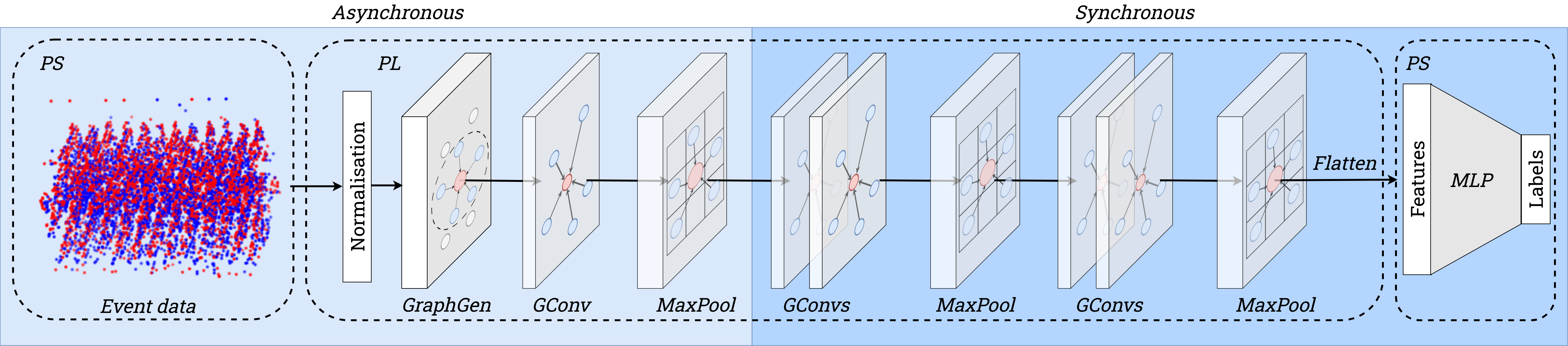
Figure 1: Overview of the proposed hardware implementation of graph convolutional networks on FPGAs specifically adapted for event data processing. The asynchronous event stream, represented as a point cloud, is received in the FPGA, where it is used to create a graph, which is then processed using a graph convolutional network accelerator for the task of object recognition.

II Prerequisites

As an introduction to the remainder of our work, this chapter outlines the fundamental characteristics of event cameras and graph neural networks, which were used in the design of our hardware accelerator.

II-A Event Cameras

A key characteristic of an event camera is its ability to capture brightness changes at the individual pixel level rather than capturing entire video frames at fixed intervals. This feature, known as asynchronicity, fundamentally distinguishes event cameras from traditional frame-based cameras.

The operation of an event camera is governed by a threshold mechanism, which determines whether the change in light intensity for a specific pixel exceeds a predefined threshold $C$. The change in light intensity is typically measured in a logarithmic scale to accommodate a wide dynamic range of lighting conditions. The process is expressed by:

$$L(u_{i},t_{i})-L(u_{i},t_{i}-\Delta t_{i})\geq p_{i}C,$$ (1)

where $L(u,t)$ represents the logarithmic light intensity at a given pixel location $u=(x,y)$ at time $t$, while $\Delta t$ indicates the time elapsed since the last event was recorded and $p$ defines the polarisation of the brightness change. The outcome of this process is an event stream that can be described as a sequence of values $E=\{x,y,t,p\}$. This method ensures that data is only captured and recorded when actual changes in light intensity occur.

One of the key advantages of event cameras is their ability to operate with very high temporal resolution of timestamps of up to 1 microsecond (1 MHz clock) and the ability to record events with an interval of up to 10 microseconds (specific values depend on the camera model, as well as the scenario under consideration). Moreover, the independent operation of each pixel in an event camera contributes to its high dynamic range (120 dB compared to 50-60 dB for traditional cameras). This makes them extremely effective in difficult lighting conditions, for example during night driving or with high illumination contrasts.

II-B Graph Neural Networks

Among many types of graph neural networks, graph convolutional networks (GCNs) have become the most common model and they are also the basis of our work. The key operation performed by GCNs is a convolution on a graph, allowing information to be propagated efficiently between vertices to update their representation and extract relevant information from the entire graph. Unlike traditional neural networks, where a layer is applied to the input data, the process of convolution on a graph is based on the mechanism of aggregation of neighbourhood information $N(i)$, that is, relations between vertices, described by a message passing scheme. It is realised by three stages: message, aggregation and update function.

In the first stage, the message function $\phi$ operates on a vertex $v_{i}$ and its neighbours $v_{j}$, determining the information between these vertices. To do so, it uses the attributes of the vertices $x_{i}$, $x_{j}$ and the edges $e_{ij}$, which is mathematically represented as:

$$msg_{ij}=\phi(v_{i},v_{j},x_{i},x_{j},e_{ij}).$$ (2)

Then, the aggregation function determines the representative information based on the collected message values from all the vertex’s neighbours $v_{i}$:

$$agr_{i}=\bigoplus_{j\in N(i)}msg_{ij}.$$ (3)

The final step is to update the vertex attributes using the update function $\gamma$:

$$\hat{x_{i}}=\gamma(agr_{i}).$$ (4)

The $\phi$ and $\gamma$ are differentiable functions, such as multi layer perceptrons (MLPs), and the operation $\bigoplus$ is a differentiable aggregating function, such as sum, mean or max value. The principles of graph convolutional networks presented here provide a general framework, while specific implementations and update mechanisms may vary, depending on the specifics of the layer. A more detailed discussion on graph neural networks can be found in the survey [22].

III Previous work

This section reviews the literature on graph convolutional networks. According to the authors’ current knowledge, which indicates that there are no publications detailing the hardware implementation of GCNs in the context of event processing, the review is divided into two segments. The first one focuses on the use of GCNs in event processing, while the second one examines the challenges of accelerating GNNs using FPGAs.

III-A Graph Convolutional Networks for Event Data Processing

TABLE I: Comparison of architectures and platforms used for event data processing by graph neural networks.

Work	Network Model	Task	Platform
Sekikawa [23]	PointNet	Semantic Segmentation and Ego-motion	CPU/GPU – Intel Core-i5
Wang [14]	PointNet/PointNet++	Gesture Recognition	GPU
Bi [15]	SplineConv	Classification	Not mentioned
Mitrokhin [16]	GraphConv	3D Classification	GPU – Nvidia GTX 1080Ti
Li [17]	GraphConv	Classification	CPU – Intel i7-9700K
Schaefer [18]	SplineConv	Classification and Detection	GPU – Nvidia Quadro RTX
Gehrig [19]	SplineConv	Detection	GPU – Quadro RTX 400
Jeziorek [24]	PointNet++	Classification and Detection	GPU – Nvidia RTX 3060

As part of the research into event processing in its original form, one of the early papers introduced the EventNet architecture [23] (modelled on PointNet [25]), which due to recursive processing enabled handling up to 1 MEPS (million events per second).

The use of the PointNet architecture was also demonstrated in the work [14], comparing it with the newer version of PointNet++ [26] and the LSTM (long-short term memory) layer [27]. Further work has also attempted to use other types of graph operations. For example, the use of the SplineConv layer [28] for vertex processing proved to be more efficient than classical CNN methods in terms of quality and computational complexity [15]. A comparison of the GraphConv layer [29] with PointNet++ also showed shorter graph processing times [16].

Of all the existing solutions, the proposals presenting the potential use of graph convolutional networks for asynchronous event processing are the most interesting. Works [17, 18, 19] solved this problem by linking events as vertices to an already existing graph and then processing them accordingly. In [17], a sliding convolution was used to propagate information between layers. On the other hand, in the works [18, 19] the graph update was carried out at the level of individual neighbours, gradually actualising a wider range of graph vertices with each layer. The presented methods show that this solution reduces the computational complexity by up to 11 times for a single event.

A different approach was presented in our previous work [30]. We noticed that the proposed solutions mainly focus on obtaining the best possible results with minimum number of operations, neglecting the memory complexity of the models and data. We have presented solutions that reduce the memory requirements, without a significant impact on the accuracy of the models.

A comparison of the architectures, together with their applications and the computing platforms used, is presented in Table I. The key observation here is that all the works use high-performance CPUs or GPUs for computation and no paper proposed a solution in energy-efficient devices, thus this is the main knowledge gap we address in this work.

III-B Hardware-Based Graph Neural Network Accelerators

To the best of the authors’ knowledge, the topic of hardware acceleration of graph neural networks for event data processing has not yet been addressed. Therefore, in this section, we present the two most closely related topics: selected works on general accelerators for graph networks on FPGAs, and point cloud data processing on FPGAs.

Dedicated hardware accelerators for GNNs on FPGAs have been developed to improve the efficiency of graph processing. In [31], a method was introduced for processing large, static graphs in smaller segments to overcome FPGA memory constraints. The study [32] focused on developing a lightweight hardware accelerator for FPGAs. A co-designed software and hardware solution was proposed to address the challenges of irregular computation and memory access in GCNs.

Other literature, such as the work [33], discusses FPGA-based accelerators for binarised GCNs, describing various hardware optimisations to significantly reduce resource usage.

In [34], an FPGA accelerator for Temporal GNNs was implemented. It updated temporal information about specific vertices and pruned vertices ‘distant’ in the context of time during the inference stage.

Additionally, there have been efforts to create FPGA accelerators specifically for processing point-cloud data. In [35], the EdgeConv layer and KNN (k-nearest neighbour) method were employed to process point clouds by finding neighbours and connecting them with edges, enabling full-fledged graph processing. A similar approach was adopted in [36], which utilised an FPGA platform for the KNN construction part of a GCN network. [37] introduces an extremely tiny framework of point cloud processing utilising pillar encoders.

The work [38] presented a hardware implementation of the PointNet architecture, achieving a processing time of 19.8 ms for 4096 points from LiDAR on the AMD Xilinx’s ZCU104 platform. Similarly, [39] implemented the PointNet architecture on an FPGA for pathfinding and obstacle avoidance in a cloud of 1400 points. However, both works processed data without creating a graph; neither vertices were interconnected by edges nor their relationships were defined.

A critical observation among these studies is the lack of focus on dynamic graph updates. Works utilising GCNs present data processing solutions where the point cloud and vertices are predetermined. In contrast, works focusing on processing data with LiDAR process the data without considering edges between vertices, which does not meet the definition of a graph and limits the relative position information between vertices. In the case of event data, it is crucial to process events asynchronously, dynamically generate the graph and utilise the relationships between vertices. The static nature of graphs and the lack of edge consideration in the current hardware acceleration approaches represent a gap that we address in this paper.

IV Method

The inspiration for the research described here was to bridge the gap between the hardware implementation of graph convolutional networks and their application in event data processing. The aim was to create a solution that takes full advantage of the information obtained from the event camera and processes it as a data stream, while minimising energy consumption. This section describes the methods used to generate graphs, convolutions and pooling on graphs, as well as the quantisation process of the model. The description covers the software implementation including hardware requirements, but a detailed description of the hardware implementation is presented in Section VI.

IV-A Assumptions

Some constraints and specifications had to be taken into account, especially having in mind the embedded hardware target following the hardware-aware algorithm design methodology. Below are the key assumptions that had a significant impact on shaping our approach:

• Asynchronous and continuous nature of the data stream: We assumed that the input data arrives as a continuous and asynchronous stream, which required the development of a methodology for efficient data preprocessing and the construction of dynamic graphs capable of handling individual events on the fly.

• FPGA platform memory limitations: Limited internal memory resources available on the FPGA platform forced us to design and implement a strategy to efficiently process the graph and its vertices through the model layers. This takes into account reducing the size of the graph to minimise the utilisation of memory. In our current approach we decided to exclude external RAM resources due to their greater latency and lower energy efficiency.

• FPGA computing precision: FPGAs are better suited to integer and fixed-point operations, as opposed to floating-point numbers, which are more complex and resource demanding. Therefore, it was important to carry out a conversion of both the model and the data being processed to numeric formats.

The remainder of this section goes on to detail the implementation of the various elements of our solution, taking into account the mentioned assumptions and hardware limitations.

IV-B Graph Construction

The following subsection briefly introduces the methodology used to generate the graphs. A more detailed description is presented in our previous work [30].

Standard method

As introduced in Subsection II-B, a graph is defined by a set of vertices $V$ and edges $E$ connecting them. Following the conventions established in the works [15, 18], the position of a vertex is represented by the spatio-temporal coordinates of the event $pos=(x,y,t)$, with the vertex attribute denoted by the polarity $x=(p)$. The generation of edges between vertices is determined by the Euclidean distance between them:

$$d_{i,j}=\sqrt{(x_{i}-x_{j})^{2}+(y_{i}-y_{j})^{2}+(t_{i}-t_{j})^{2}}\leq R$$ (5)

where $d_{i,j}$ represents the distance between vertices at positions $pos_{i}=(x_{i},y_{i},t_{i})$ and $pos_{j}=(x_{j},y_{j},t_{j})$. $R$ represents the threshold distance for edge generation. Given the much smaller size of the temporal values compared to the spatial values, time normalisation is initially applied to adjust its scale to the spatial dimensions. Furthermore, in order to reduce the generation of an excessive number of edges, their maximum number is limited to $D_{max}$ per event.

Our Graph Generator

The direct search for neighbouring vertices within the entire set of vertices poses significant computational and memory challenges for hardware implementations. To address them, we propose a hardware-aware graph generator.

Initially, both spatial and temporal values are normalised simultaneously to ensure uniform scaling, and then they are projected to integer values. The normalisation process is formalised as follows:

$$x_{i}^{*}=\left\lfloor\alpha\cdot\frac{x_{i}}{W}\right\rfloor,\quad y_{i}^{*}=\left\lfloor\alpha\cdot\frac{y_{i}}{H}\right\rfloor,\quad t_{i}^{*}=\left\lfloor\alpha\cdot\frac{t_{i}}{T}\right\rfloor,$$ (6)

where $\alpha$ is the normalisation factor, $W$ and $H$ represent the spatial resolution and $T$ represents the time window of events.

The next step is to use a neighbourhood matrix (NM) to generate edges. This matrix, with dimensions corresponding to the normalised spatial resolution of the data, stores the most recent event time value for each pixel. For each event, the temporal values in radius $R$ are searched, and if the distance condition (5) is satisfied, the event is considered a neighbour, and a directed edge is generated from the event stored in the matrix to the new one, with the temporal value in the neighbourhood matrix updated.

This approach allows the graph to be updated asynchronously and dynamically for each event. Furthermore, as we have shown in our work [30], such a modification does not significantly affect the performance (loss of accuracy of 0.08% in the detection task for the N-Caltech101 dataset).

IV-C Graph Convolution

We focus on the application of the PointNet++ like architecture, among different types of convolution used to process the data. This selection was guided by our prior research [24], in which we achieved a notable reduction in the size of the representation and model.

The PointNet++ model is designed to efficiently process vertex features in 3D point clouds, implementing the transformation defined by the equation:

$$\hat{x_{i}}=\gamma\left(\underset{j\in N(i)}{\max}\phi(x_{j},p_{j}-p_{i})\right)$$ (7)

where $\phi$ is a local function that processes the vertex attribute $x_{j}$ and the relative spatial coordinate $p_{j}-p_{i}$. The operator $max$ selects a representative attribute based on the information received from the neighbours $N(i)$, while $\gamma$ is a global function that updates the attribute of vertex $i$ and is optional.

The choice of the PointNet++ architecture is primarily due to its inherent suitability for point cloud data and its ability to operate without defining edge attributes in contrast to the SplineConv model, which simplifies the data representation (as demonstrated in our earlier work [24]).

Convolution in our study is defined as an operation that transforms information from the input dimension $in_{ch}$ to the output dimension $out_{ch}$, determining the size of the vertex attribute. The function $\phi$ is understood as a simple linear transformation, mapping values from the dimension $in_{ch}+3$ to $out_{ch}$ ($+3$ is due to the spatio-temporal dimension of the events). The $\gamma$ function is not included to reduce the complexity of the model.

IV-D Graph MaxPool

MaxPool on graphs is a technique for reducing the number of vertices in a graph. It is particularly useful in deeper layers of neural networks, where the size of attributes can increase significantly, as it reduces the number of operations required. The technique involves partitioning the data space into uniform $C_{k}$ clusters. For each of these clusters, a new vertex is selected whose attribute value corresponds to the maximum attribute value among all vertices in the cluster, which can be represented by the equation:

$$x_{k}=\max_{i\in C_{k}}x_{i}$$ (8)

while the position of the new vertex is determined as the average of the positions of all vertices in the cluster:

$$pos_{k}=\frac{1}{|C_{k}|}\sum_{i\in C_{k}}pos_{i}$$ (9)

In this process, connections that link vertices from distinct clusters are merged into a single edge between new points, eliminating repeated connections and those internal to the groupings.

In our study, in order to adapt to the hardware constraints and provide fixed-point numbers, instead of calculating the average position, which could be a floating-point value, the position of the new vertex is defined as the index of the cluster. In other words, the value is divided by the cluster size $g$ and converted to an integer value, as shown below:

$$pos_{k}=\left\lfloor\frac{pos}{g}\right\rfloor$$ (10)

This approach creates a simplified graph structure through which the number of vertices and edges is reduced. The vertex locations are rescaled to a range from 0 to $\frac{\texttt{SIZE}}{g}$ in each spatial dimension, where SIZE represents the size of the data space before MaxPool reduction is applied. This simplifies graph management in the context of hardware constraints, and also contributes to computational efficiency in deeper layers of the neural network.

IV-E Model quantisation

The hardware implementation of graph convolutional networks requires consideration of the model quantisation process, which plays a key role in optimising resource consumption and computational efficiency. To achieve this goal, we used the Quantisation Aware Training (QAT) technique, based on the integer-arithmetic-only matrix multiplication quantisation scheme presented in [41]. We applied the quantisation process to the $\phi$ activation function in the convolution layer and input data.

For the first convolution in the message function, both input features of events $x$ and position differences $pos_{diff}$ are quantised, which are then processed by the linear layer with quantised weights and bias. The output features after the message function are then subjected to an aggregation operation.

An important difference, however, is that the output from the first convolution cannot be directly passed to the second convolution, as it also requires a quantised position difference. Therefore, for each subsequent convolution we only quantise the position difference and merge it with the previous output. And since the position values at graph generation and during MaxPool operations are projected to integer values, position differences also belong to this domain.

TABLE II: Details of statistics and preprocessing parameters for the datasets used, including N-Cars (N-C), N-Caltech101 (N-Cal), CIFAR10-DVS (C-DVS) and MNIST-DVS (M-DVS).

Datasets	N-C [42]	N-Cal [43]	C-DVS [44]	M-DVS [45]
Samples	24029	8246	10000	30000
Classes	2	100	10	10
Duration	100 ms	300 ms	1280 ms	2-3 s
Resolution	$120\times 100$	$240\times 180$	$128\times 128$	$128\times 128$
Normalisation $\alpha$	128	256	128	128
Time Window	100 ms	50 ms	100 ms	100 ms

V Experiments

This section presents the results of the evaluation, in particular the impact of the solutions used on the final classification performance. We discuss the used datasets, summarise implementation details and present comparisons with other solutions reported in the literature.

V-A Datasets

In our experiments, we focused on the object classification task from events. This is a standard setup that enables us to evaluate the proposed solution, especially in hardware. Moreover, many solutions that utilise graph convolutional networks for event processing focus on object classification, allowing us to compare the results with them. We selected four commonly used datasets collected using event-based cameras: N-Cars [42], N-Caltech101 [43], CIFAR10-DVS [44], and MNIST-DVS [45].

The details about the dataset statistics and the parameters used during preprocessing are summarised in Table II. Since the N-Caltech101, CIFAR10-DVS and MNIST-DVS datasets do not have a clearly defined test set, we split the training set in a ratio of 80:20. Following the work [18], for the N-Caltech101 dataset, we selected events within a time window of 50 ms from each sample and for the N-Cars dataset, we used the entire sample length, i.e. 100 ms. For the CIFAR10-DVS and MNIST-DVS datasets, we cut 100 ms from the samples to reduce the number of events processed for a single graph. According to Equation (6), the CIFAR10-DVS, MNIST-DVS and N-Cars data was normalised with $\alpha=128$, while in case of the N-Caltech101 $\alpha$ was set to $256$.

TABLE III: Comparison with other methods in the object classification task. Although our accuracy does not exceed state-of-the-art levels, we show that our solution has relatively small performance losses. The size and accuracy of our models is determined after quantisation with 8-bit accuracy. EFGCN uses smallest number of parameters, resulting in an extremely compact model size suitable for FPGA implementation.

Model	Representation	N-Cars	N-Caltech101	CIFAR10-DVS	MNIST-DVS	Size [MB]	Param [M]
EV-VGCNN [46]	Voxel	0.953	0.748	0.670	-	3.20	0.84
VMV-GCN [47]	Voxel	0.932	0.778	0.690	-	3.28	0.86
VMST-Net [48]	Voxel	0.944	0.822	0.753	-	3.61	0.95
G-CNNs [15]	Graph	0.902	0.630	0.515	0.974	18.81	4.93
RG-CNNs [15]	Graph	0.914	0.657	0.540	0.986	19.46	5.10
NvS-S [17]	Graph	0.915	0.670	0.602	0.986	-	-
EvS-S [17]	Graph	0.931	0.761	0.680	0.991	-	-
AEGNN [18]	Graph	0.945	0.668	-	-	83.31	21.84
$\text{OAEGNN}_{R=3}$ (our)	Graph	0.903	0.601	0.502	0.911	0.82	0.86
$\text{OAEGNN}_{R=5}$ (our)	Graph	0.928	0.645	0.541	0.942	0.82	0.86
$\text{EFGCN}_{R=3}$ (our)	Graph	0.853	0.576	0.478	0.892	0.40	0.42
$\text{EFGCN}_{R=5}$ (our)	Graph	0.896	0.619	0.498	0.904	0.40	0.42

V-B Software Implementation Details

In the study, we propose two models. The first one, namely OAEGNN (Optimised-AEGNN), serves as a benchmark to evaluate the impact of our methodologies on both model size and accuracy results obtained. Drawing inspiration from the architecture of AEGNN [18], which is one of the most recent developments that uses graph convolutional networks for object classification, OAEGNN consists of seven convolutional layers and two MaxPool layers. However, it is important to note that this model is not inherently suitable for direct hardware implementation on FPGAs, as it does not meet certain implementation assumptions. In particular, the inclusion of the MaxPool layer at later stages of the model and the addition of two residual connections requires significant memory allocation, potentially requiring the use of external RAM. Therefore, the OAEGNN model is primarily used to evaluate the performance of our approach against state-of-the-art solutions.

We therefore introduce a second model, EFGCN (Event-Based, FPGA-Accelerated, Graph Convolutional Network), a smaller variant of the OAEGNN model, explicitly tailored for hardware acceleration on FPGAs. The model consists of five convolutional layers and three MaxPool layers, where the details are shown in Figure 1. Due to the early integration of the MaxPool layer in the model, its adaptation to hardware implementation is facilitated and also, as highlighted by the authors of [19], overall network performance is improved. In addition, the EFGCN model has been designed for reduced resource consumption, ensuring compatibility with a wider range of FPGAs beyond the Xilinx UltraScale+ ZCU104 utilised in our study. While classification accuracy is a factor in our benchmarking analysis, it should be noted that these results do not represent the full potential achievable on our platform. The scalability of the model is explained in the dedicated Section VI-D.

In both models, after each convolution, the ReLU activation is applied. As a classifier for each model, we used a single fully connected layer (FC) with the number of outputs corresponding to the number of classes in a particular dataset. In order to reduce overfitting, we added a dropout layer with probability $0.3$ between the output MaxPool and the FC layer.

For each dataset and model, we implemented a neighbour search within a radius $R$, equal to 3 and 5.

The float model was trained using the AdamW optimiser [49] for 50 epochs, using cross-entropy loss, with the batch size equal to 16. The learning rate was set to value betwen $10^{-3}$ and $10^{-4}$ based on the dataset and the weight decay parameter was equal to $1\cdot 10^{-3}$. After 50 epochs, we trained the model using the Quantisation Aware Training method for further 20 epochs, with the same learning parameters. For augmentation, we randomly flipped the events horizontally and rotated them relative to the XY axis by 10

The implementation of the model and event processing was fully developed using the PyTorch library and Numpy. For the code and more information, please visit the project page: https://github.com/vision-agh/***.

V-C Comparison with other models

To assess our methodologies and software implementations, we evaluated them against two main criteria. The first is the accuracy metric, which measures classification performance. The second criterion relates to the size of the model and the number of its parameters as shown in Table III.

We included models using graph-based event representations, such as G-CNNs/RG-CNNs [15], NvS-S/EvS-S [17], and AEGNN [18], detailed in Section III-A. In addition, we evaluated methods such as EV-GCNN [46], VMV-GCNN [47] and VMST-Net [48], which generate voxels from events.

The sizes of the models were estimated based on the number of parameters, defaulting to 32-bit floating-point in the case of no explicit information. For our models, the precision after quantisation was set to 8 bits for weights and 32 bits for biases.

The EV-VGCNN, VMV-GCNN and VMST-Net methods provide significant accuracy using a sparse event structure, with a number of parameters comparable to our OAEGNN model. Unlike graph-based methods, these approaches transform events into voxels within a specified time window and then select representative voxels for processing. As a result, only a fraction of all events are used, and the voxelisation of events makes the asynchronicity process difficult for hardware implementation.

The results of our OAEGNN model compared to the original AEGNN architecture show differences of 1.7% for the N-Cars and 2.3% for the N-Caltech101. In addition, for the N-Cars we outperform the G-CNNs, RG-CNNs and NvS-S models, and the results are comparable to the EvS-S and VMV-GCN models. For the CIFAR10-DVS, our model outperforms both the G-CNNs and RG-CNNs. It was possible to achieve such results even with more than a 100-fold reduction in model size compared to AEGNNs and about 23-fold reduction relative to G-CNNs and RG-CNNs models.

In contrast, the results for the EFGCN model show a reduction in accuracy compared to the OAEGNN model. When analysed for a radius of $R=3$, a decrease in accuracy of 5% for the N-Cars, 2.5% for the N-Caltech101, 2.4% for CIFAR10-DVS and 1.9% for MNIST-DVS was observed. However, it should be emphasised that the EFGCN model was designed as a proof-of-concept for a hardware implementation of a graph convolutional network after applying the proposed optimisation methods and is a starting point for further research on the scalability of the solution.

Summary of the results

Our work demonstrates that the application of our methods significantly reduces the size of the models without drastically affecting the accuracy of the results. Additionally, we are capable of performing asynchronous updates of events, and implementing these on an FPGA is feasible. While our models do not achieve state-of-the-art classification accuracy, achieving this was not our primary objective. Although other studies present better results, their models run on large GPUs and are not directly applicable to FPGAs due to their larger size.

It should also be noted that our models are of miniature size and follow the TinyML trend, which has an impact on their efficiency. However, the models we present do not represent an upper limit of performance. There are several pathways that can lead to significant improvements in performance. Foremost is the ability to design a larger model that makes better use of the FPGA chip’s resources. One of the most promising and constantly evolving techniques is knowledge distillation [50, 51], which allows a small model, called the student, to benefit from the knowledge of a larger model, called the teacher. This method fits perfectly with our work on hardware optimisation and offers great hope for future improvements. Therefore, these ideas will be investigated in our future research.

VI EFGCN Implementation on SoC FPGAs

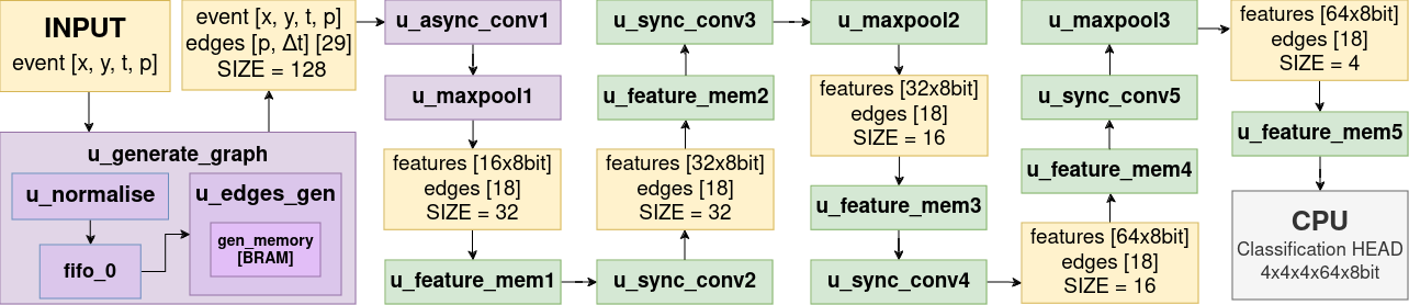
Figure 2: Schematic of the EFGCN network hardware modules for $R=3$ and N-Cars classification (the asynchronous part – violet and the synchronous – green). The characteristics of data transferred between the selected modules are highlighted (yellow blocks).

Based on the methods of model optimisation described in Section IV, we proceeded to realise a proof-of-concept for the implementation of graph convolutional networks for SoC FPGAs. We implemented and synthesised the EFGCN model for N-Cars classification for the Zynq UltraScale+ MPSoC ZCU104 Evaluation Kit using Vivado 2022.2 software.

We designed the hardware architecture as a pipeline of modules implementing successive layers of a graph convolutional network that process data in a completely parallel manner – each layer can process data simultaneously, as long as its input data is available. The system consists of two parts – asynchronous (operating in an event-by-event manner) and synchronous, in which operations are performed on sub-graphs (see Figure 1). The toolchain can process any length of the sequence of events recorded by the camera continuously, generating a prediction at the output for data recorded during the last TIME_WINDOW (duration of a single sample of event data sufficient to perform the classification). The system assumes the use of a SoC FPGA platform, where feature extraction is implemented in the programmable logic and the network head is realised in software.

For real-time functionality, the module needs high throughput, determined by clock frequency and maximum operation latency per event. Higher frequencies increase system throughput but can introduce timing challenges (requiring synchronous operations between rising edges of clock signal) and increase power consumption. The proposed graph convolutional network acceleration module processes events one by one, and its throughput can be determined by the maximum number of events per second. The data collected within a certain time window (50 ms for N-Caltech101 and 100 ms for N-Cars) is represented as a graph of SIZE $\times$ SIZE $\times$ SIZE. The theoretical maximum number of events per unit time (TIME_WINDOW divided by SIZE) is therefore SIZE $\times$ SIZE. However, it should be noted that event data is sparse in nature and considering the theoretical maximum number of events misses the point. To estimate realistic throughput requirements, the maximum number of events per unit time in each dataset was examined – 1.35 MEPS for N-Caltech101, 0.59 MEPS for N-Cars, 0.34 MEPS for CIFAR10-DVS and 0.063 MEPS for MNIST-DVS.

To ensure that such throughput requirements are met, we identified the operation with the highest latency, i.e. the bottleneck of the system – the memory accesses for searching the edges of the graph. For this purpose, we use URAM and BRAM, which have deterministic and constant latency. The number of accesses depends on the radius $R$, which determines the size of the context to be searched. For the purpose of experiments in hardware, $R=3$ was assumed, i.e. 29 edge candidates (see Section VI-A). To reduce the throughput we used dual-port memories to minimise the number of reads. The maximum latency in the system is therefore 15 clock cycles.

For further work, a clock frequency of 200 MHz was chosen to ensure low latency while still meeting the above requirements. Consequently, the system can accept a new event every 75 ns (15 clock cycles), which corresponds to a throughput of 13.3 MEPS (much higher than calculated for any of considered datasets). The throughput calculated in this way was confirmed by simulation.

In the following sections we present the functional description of the hardware modules used. Implementation details can be found in the supplementary material. The topic of the scalability of the accelerator is described in Section VI-D.

VI-A Description of the hardware modules

This section describes each hardware module used in the system, preserving their order in the system pipeline. A diagram of the accelerator pipeline with all modules highlighted can be found in Figure 2.

Graph generation

Events recorded by the camera are transmitted to the input of the hardware module in real-time – consistent with their timestamps. The number of events per time unit depends on the dynamics of the scene. The first of the hardware modules in the system’s pipeline is u_generate_graph (described, prior to the optimisations for this system, in our previous paper [30]).

As a first operation, the event’s $x$, $y$ and $t$ values are rescaled to 0 - SIZE (for N-Cars – 127) in u_normalise module to limit the resources used to store them. After normalisation, the events are written to a FIFO queue implemented in BRAM (fifo_0) to ensure correct operation at moments of increased dynamics of the observed scene (events generated more frequently than every 75 ns – the designated system throughput).

Events from the FIFO queue are read by the edges generation module (u_edges_gen), whose task is to connect the vertices (events) by edges. It is based on a two-port BRAM, which stores information about the context – last recorded events for each coordinate $x$ and $y$ – module gen_memory [BRAM] in Figure 2. For each event read from the queue, a context is read from the memory – 29 surrounding values. For each read, the semi-sphere condition is checked (Equation (5)). Next, the currently processed event is written to the context. This operation, due to the use of dual-port memories, requires 15 $READ$ operations on one of the ports, and 14 $READ$ operations and one $WRITE$ operation on the other (the aforementioned bottleneck in the implemented system).

We also implemented a ‘drop’ mechanism – in case the processed event is a duplicate i.e. a registered event with the same values $x$, $y$ and $t$ after normalisation, it is dropped. Once the context analysis is complete, the module’s outputs are generated: pairs of vertices ($x$, $y$, $t$, and $polarity$), and a vector describing their edges (including their polarity).

Asynchronous convolution

Successive pairs of vertices and their edges appear at the module’s input asynchronously with preserved order – no more frequently than once every 15 clock cycles, but with an unknown time span (depending on the dynamics of the observed scene). For each incoming value, a graph convolution (module u_async_conv1) is performed, described in detail in Section IV-C. It consists of a sequence of matrix multiplication operations of successive feature maps and weight matrices performed for each edge of the processed vertex and additionally for the vertex itself (so-called ‘self-loop’).

For the first convolution, the feature matrix consists of 4 elements – an attribute (the polarity $p$ of the vertex connected by an edge to the vertex being processed) and the difference of the positions of the connected vertices in the three coordinates ($x$, $y$ and $t$). For ‘self-loop’, the position is fixed at $(0,0,0)$ and the attribute is the polarity of the vertex being processed. No extra memory is required, since the described initial convolution processes only the values that are already present in the module’s input. To conserve resources, we perform sequential operations with two matrix multiplication modules (up to 29 multiplications + self-loop, across two parallel modules in 15 clock cycles). This operation is realised using LUT resources (without DSP multipliers) due to the small number of bits representing the values. Important at this stage, however, is the quantisation of the values as described in Section IV-E. For this purpose, look-up tables, bit-shifting and multiplication using DSP modules are used (see the supplementary material for a detailed description).

The resulting vectors from the multiplication for each edge (and self-loop) are compared with an element-wise maximum operation (taking into account layer-specific minimum values – ReLU activation). This generates the final feature map vector, which is propagated to subsequent model layers. The output of the u_async_conv1 module is the currently processed vertex and its edges (delayed by an appropriate number of clock cycles) and a vector of calculated features for that vertex.

‘Relaxing’ MaxPool

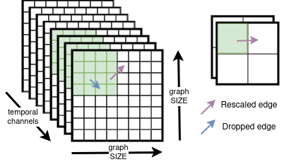
Figure 3: ‘Relaxing’ MaxPool of size $4\times 4$. As a result of the graph scaling, all vertices in the $4\times 4$ area are represented by a single vertex (green area). Consequently, the resulting graph is 4 times smaller along each axis. The number of edges is also reduced. Those that point to themselves after the MaxPool operation (blue arrow) are discarded. Only those edges which, after scaling, connect vertices located in different areas (violet arrow) remain.

Crucial due to the limited memory and logic resources is the use of the proposed ‘relaxing’ MaxPool module (u_maxpool), which makes it possible to significantly reduce their demand in the system. As described in Section IV-D, the module aims to scale the entire graph along the $x$, $y$ and $t$ coordinates (see Figure 3). Since, after scaling, a single vertex can represent more than one event, their order in the rest of the system is disrupted and output vertices can be processed by subsequent layers only after their accumulation for the entire set of temporal channels. Thus, the MaxPool module splits the accelerator into two parts: asynchronous (event-by-event processing) and synchronous, where data is processed in ‘temporal channel-by-temporal channel’ manner. This method has the effect of severely ‘relaxing’ the timing requirements further down the system. For example, for the EFGCN model and the N-Cars dataset, a TIME_WINDOW of 100 ms was assumed. After the MaxPool operation, the graph has a SIZE equal to 32. This means that the next ‘temporal channel’ of the graph is generated every 3.125 ms (equivalent to 625 200 cycles of the 200 MHz clock).

After scaling, the MaxPool layer writes a feature map for a given vertex and an array of its edges to memory addressed using $x$ and $y$ (described in the next section). The vertex’s feature map is the result of the element-wise maximum operation performed for each of the feature maps represented by that vertex (for that purpose, a memory READ is required to verify previous feature maps). Due to the use of MaxPool $4\times 4$, in the synchronous part, possible distances of edges in each direction are $\{-1,0,1\}$, and their maximum number is reduced to 17. Due to the use of directed graphs, for a given vertex, its edges are either in the acutely processed ‘temporal channel’ or in the most recent previous one.

Feature memory

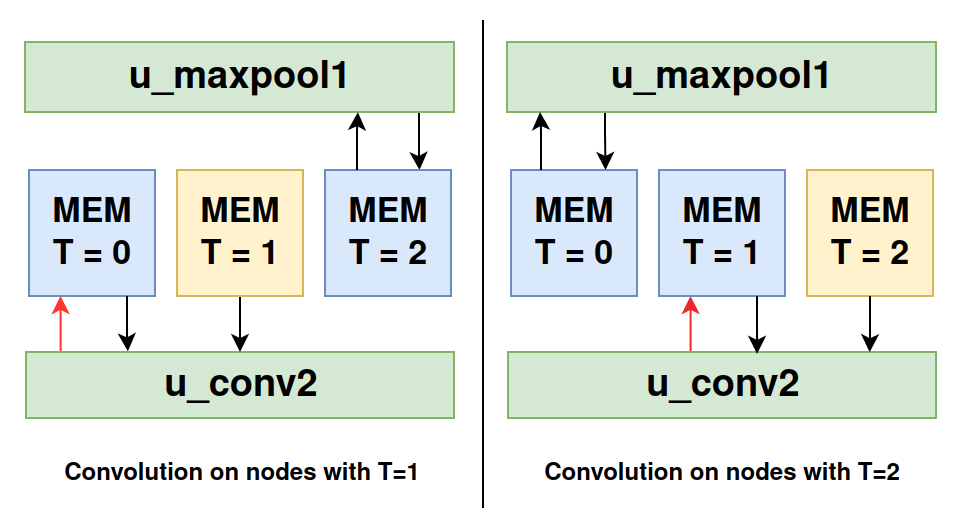
Figure 4: Visualisation of the memory switching method. While the convolution layer reads consecutive vertices from memory T=1 and neighbours from the memories T=1 and T=0 respectively, the MaxPool layer writes data to memory T=2. The red arrow points to the memory that will be reset after the convolution. Once the operations are complete, a memory switchover takes place. MaxPool becomes connected to the zeroed memory T=0 and u_conv2 to the memory with current events T=2 and past events T=1.

In order to limit the necessary memory resources for the implementation of the system, we standardised their use in the synchronous part. Between each MaxPool module and the convolution, and between the consecutive convolutions, a u_feature_memory module is instantiated. Inside, there is a memory shared between consecutive layers which consists of three independent BRAM modules, with dimensions SIZE $\times$ SIZE each (addressed by vertex coordinates). It is worth noting that the value of SIZE varies from layer to layer – it refers to the current size of the graph (after the MaxPool, the SIZE is changed). Each memory element is a feature vector of appropriate length and an edge vector for a vertex with given coordinates.

We use three independent memories due to the characteristics of the system. While the MaxPool layer uses one of these, the subsequent convolution layer uses the other two (as illustrated in Figure 4). Once the MaxPool has been executed for all vertices in a given ‘temporal channel’, a memory switchover is performed. In this way, the number of necessary memory cells is kept to a minimum and shared by the subsequent layers.

Synchronous convolution

In the synchronous part of the system, convolutions are realised for the entire ‘temporal channels’ of the graph (the u_sync_conv modules). The required bandwidth of the convolution module is dependent on the hyperparameters – TIME_WINDOW for the whole system, the clock frequency and SIZE for a given convolution. For the first synchronous convolution in the EFGCN model for N-Cars, the operation must be performed for all vertices from a $32\times 32$ (1024 elements) memory. For each vertex, it is necessary to realise 9 $READs$ (one for each possible vertex coordinate, from two memories in parallel – currently processed and the previous one – 18 feature vectors). For this task we have 100/32 ms available, i.e. 625 200 clock cycles (see ‘Relaxing’ MaxPool).

To limit resources, we decided to perform successive multiplications in a sequential manner. The first sequential convolution module used (u_sync_conv2) implements $16\times 32$ convolution – so it generates a map vector of 32 elements of size unsigned 8-bit. The multiplication should be performed $32\cdot 32\cdot 9$ times (SIZE $\times$ SIZE $\times$ the number of reads from memory for a single vertex). Due to the relatively large value of TIME_WINDOW and the low resolution of the N-Cars set, it was decided to perform the operation in 32 steps (each element of the output feature map separately). The matrix multiplication module was therefore replaced by a vector multiplication module, whose mode of operation (including quantisation) is analogous to asynchronous convolution. The DSP modules used have been significantly reduced in this way – for each output element, the scaling for quantisation is done sequentially rather than in parallel. Multiplication realised in this way requires 294 912 clock cycles ($32\times 32\times 9\times 32$), so it meets the required time constraint (625 200 clock cycles).

We implemented further part of the graph convolutional network acceleration system using the same modules already described. For each convolution, we calculated the required throughput and the ability to perform part of the calculations in a sequential manner. In the described architecture for N-Cars, all sequential convolutions meet the throughput requirements using vector multiplication rather than matrix multiplication.

TABLE IV: Resource utilisation for EFGCN model on ZCU104 platform for N-Cars dataset.

Module	LUT	LUTRAM	FF	BRAM	DSP
GCN accelerator (sum)	51980	1337	16603	176.5	88
GCN accelerator (usage)	23%	1%	4%	57%	5%
u_gen_graph	516	24	372	5.5	0
u_async_conv1	5855	138	1166	0	64
u_maxpool1	698	131	750	0	0
u_feature_mem1	538	0	12	13.5	0
u_sync_conv2	3772	63	1560	2.5	6
u_feature_mem2	667	0	12	24	0
u_sync_conv3	7522	63	2269	4.5	6
u_maxpool2	924	259	1013	0	0
u_feature_mem3	1514	0	10	24	0
u_sync_conv4	6936	72	2836	4.5	6
u_feature_mem4	1819	0	10	45	0
u_sync_conv5	10879	72	4271	8	6
u_maxpool3	1561	512	1721	0	0
u_feature_mem5	1556	0	6	45	0
u_out_serialize	165	0	559	0	0

VI-B Implementation results

After simulation, the graph convolutional network accelerator was implemented and evaluated in terms of resource utilisation, latency and estimated power usage for the ZCU104 platform. For 200 MHz clock, all specified timing constraints were met ensuring correct operations.

Utilisation

The resource utilisation of the ZCU104 platform is presented in Table IV. We used 57% of the BRAMs (none of the 96 available URAMs were used despite being supported for each u_feature_map module). The utilisation of DSP multipliers is low due to the sequential implementation of multiplication for synchronous convolutions. The consumption of logical resources increases significantly for successive layers of synchronous convolution (as the size of the input feature maps increases). However, it is possible to implement part of the multiplication operations on the DSP, the consumption of which is only 5%. In summary, the proposed model does not make the full use of the resources available on the ZCU104, and the potential of this medium-sized SoC FPGA platform has not been fully exploited. We conclude that the accelerator designed in this way can be deployed on a smaller FPGA or used to implement larger models (see Section VI-D).

Latency

The accelerator allows the next prediction to be determined at the output for the last 100 ms based on the last four ‘temporal channels’ after the generation of each one (the last MaxPool module scales the graph to size $4\times 4\times 4$). The overall output generation time was therefore measured using the time between the reception of the first event at the system input and the generation of the first ‘temporal channel’ at the output as 29.47 ms. It should be emphasised, however, that the results obtained can be considered satisfactory due to the fact that the single output ‘temporal channel’ represents data obtained over a period of 25 ms (100/4 ms). Consequently, it can be established that the overall system latency (defined as the time between the registration of the last input in a given output ‘temporal channel‘ and its generation) is 4.47 ms.

Power consumption

Using Vivado tools, the implemented accelerator was subjected to an analysis of the power consumption. The maximum total on-chip power was estimated at 2.798 W (0.844 W device static and 1.955 W dynamic). However, it should be noted that the actual event data is sparse in nature, which significantly affects the actual power consumption.

Comparison with other works

The achieved implementation results can be compared with other works addressing similar issues. However, this task is made difficult by the fact that, to the best of the authors’ knowledge, the presented solution is not only the first one addressing the topic of FPGA acceleration of graph convolutional network for event cameras, but also treating FPGA acceleration of PointNet++, thus addressing the topic of local dependencies between point cloud elements (graph edges).

The most similar solutions are those that target PointNet accelerators for 3D point cloud data, which are significantly simpler (no edges connecting points). The work of [38] presents an FPGA-based PointNet accelerator for LiDAR data in automotive context realised for the same platform – ZCU104. The solution uses an architecture for classification consisting of two convolution layers and one MaxPool layer. However, the data is processed as an entire graph (not in an event-by-event manner). The authors report a latency of 19 ms for a $64\times 64$ graph (4096 vertices), while the latency of our solution can be determined as 29.47 ms for a graph fragment with a maximum number of vertices equal to 524 288 ($128\times 128\times 32$). At the same time, the accelerator [38] uses significantly more FPGA resources – 19530 LUTs (37% of our solution utilisation), 36101 FFs (217%), 1026 DSPs (1166%), and 114 BRAMs and 48 URAMs (relative to 176.5 BRAMs and no URAM usage in our system).

Similarly, PointNetLK network accelerator (also without graph edges) for 3D point cloud data has been implemented for ZCU104 in [52]. In this work, the data is processed point-by-point through a model consisting of 6 convolution layers and one MaxPool. The reported latency of the solution is 366 ms for a graph of size $1024\times 1024$. The latency is thus 10 times higher, for a graph twice the size. Depending on the optimisations made in the model, the reported utilisation of available BRAMs ranges from 27% to 55% (our solution – 57%). At the same time, however, significantly more DSP modules are used (from 12% to 48.5% of available). A very low power consumption of only 722 mW is worth mentioning.

Our system can be also compared with other works addressing event-based classifiers implemented for FPGA acceleration. In [21] ESDA, a sparse CNN data-flow architecture is evaluated on N-Caltech101. The accuracy of 72.4%, achieved with a latency of 3 ms by a memory-hungry network, is an impressive result, however, it could not be implemented for a medium-sized FPGA (1792 DSPs, 1278 BRAMs, 154K LUTs), which precludes an application in an embedded context. The paper [53] reported performance results of 72.3% for the N-Caltech101 dataset with the use of nearest-neighbour temporal filtering and sub-sampling, feature extraction based on custom descriptor (PCA-RECT) and simple feature matching and classification based on k-d trees + SVM (support vector machine) algorithm. The reported solution has significantly lower resource utilisation relative to ours (35% LUTs, 27% BRAMs and 4% DSPs). The obtained latency (560 ns for a single event) and power consumption (0.37 W) are also low. However, it is worth noting that the proposed method does not use neural networks, but simple classical machine learning methods, which tend to have low scalability for more complex problems (e.g. object detection) and for more dynamic scenarios, where graph networks achieve high results (as indicated in e.g. [19]).

VI-C PS-PL communication and network head

In order to test the performance of the hardware architecture on the target SoC FPGA platform, it was necessary to pass an event stream to the module’s input and receive its output set of features, determined in a given ‘temporal channel’.

The most desirable solution would be a direct connection of the camera with the appropriate port of the SoC FPGA platform. Unfortunately, the manufacturer of the camera we use (EVK1 model from Prophesee with USB 3.0 output interface) does not provide any information regarding the low-level operation of the device. Therefore, we saved data from the camera to a text file (in the form of events, as described in Section II-A) and then read it from an SD card placed on the hardware platform. This part was realised in the Vitis 2022.2 environment on the processor side, which sends event data via the AXI4 bus (with burst support) to the programmable logic, where the described EFGCN hardware architecture was implemented. To simulate real occurring timestamps, appropriate delays were set between sending successive events.

Once the computations in the GCN accelerator (programmable logic) are finished, the extracted features can be used for many different tasks, including, for example, object classification. Due to the relaxed throughput, we decided to implement the network head on the processor side to make the solution versatile. The resulting feature vectors are passed to the function (on the processor) that performs the linear layer functionality and selects the index of a maximum value, which is equivalent to the class index of the classified object.

The feature vector received from the logic part was identical to the vectors obtained in both the software model and the simulation in Vivado environment, thus confirming the correctness of the accelerator operation on a selected ZCU104 platform. To process the events from 100 ms time interval 113 ms were needed – the additional delay was introduced by sending the events from the processor to the logic part with simulated timestamps, the latency of the accelerator module, receiving the feature vector from the logic part and performing the linear layer on the processor side.

Due to the additional logic for communication, the resource utilisation increased by a negligible amount of 925 LUTs (0.4% of total resources on ZCU104), 2308 FFs (0.5%), 0.5 BRAMs (0.2%) and 0 DSPs. Power estimation calculated in Vivado software for the entire architecture is 4.85 W – the additional energy is consumed by the processor and elements responsible for the communication.

VI-D Scalability

The accuracy scores achieved for the EFGCN model differ from state-of-the-art for each of used classification datasets. At the same time, in Section V, it was proven that the proposed optimisations themselves have little impact on the accuracy. Its decrease is therefore a result of the relatively small size of the model used. Thus, an important issue to address in the context of the proposed accelerator for graph neural networks using event data is its scalability, i.e. whether it can also be applied to bigger models.

Impact of input graph size and TIME_WINDOW

Section V considers tests of the proposed model for the N-Caltech101 set, which has a higher data resolution. To ensure the correct classification for this dataset we use a TIME_WINDOW of 50 ms and an input graph of SIZE $=256$. As the size of the input graph grows, the SIZE value for the entire system also increases, leading to greater demands for memory resources. Moreover, adaptation of the proposed model for a set with other hyperparameters requires a re-analysis of the throughput for sequential convolutions. The relevant calculations for acceptable sequential multiplications are comprehensively described in the supplementary material. We have estimated that for twice as big graph and two-time smaller time window, the accelerator can be implemented with 202 BRAM modules, 4 URAM modules and 184 DSPs, which is still appropriate utilisation for a medium-sized FPGA like the one available on ZCU104 platform. It is worth noting that logic resources utilisation increases proportionally as well. However, it should be remembered that it is possible (if necessary) to reduce the LUTs utilised for matrix multiplication by implementing some of these operations using available DSP multipliers.

Impact of edge search radius

From the experiments described in Section V, it appears that the accuracy of software models for classification increases when the search radius of vertex edges is increased. Implementing the network for $R=5$ using the designed accelerator is possible but involves certain consequences. First of all, increasing the neighbourhood significantly affects the throughput of the whole system – the latency of the bottleneck, which is the graph edge generation. While for $R=3$ the number of possible edge candidates is 29, for $R=5$ it is already 81. For a 200 MHz clock, the system throughput drops to a value of 4.88 MEPS. The number of edges in sequential part also changes (49 after first MaxPool, 17 after the second one) and as a result the number of DSP modules used increases (due to the smaller possible number of sequential multiplications). Increasing the number of edges also affects memory resources (marginally, as its use by feature maps is significantly greater than by edge information). We plan further work to implement the accelerator for increased radius values. We consider two solutions: parallelise memory reads for improved throughput and implement a multi-clock domain system increasing speed of memory operations for asynchronous part of the accelerator (e.g. 300 MHz clock).

Impact of additional layers

When designing the network architecture, its size should be a compromise between desired performance and the resources available on the hardware. As a reference, an estimation of resource utilisation was carried out for significantly larger two models: one inspired by work [24] (11 Conv and 4 MaxPool layers), where PointNet++ was first used for object detection and classification of event data and the other inspired by [19] (10 Conv and 4 MaxPool layers) where the state-of-the-art accuracy for object detection on event data with a graph network was established.

For the calculations (described in detail in the supplementary material) we assume the classification for N-Caltech101, i.e. a time window of 50 ms and a graph size of 256. The resulting estimated utilisation for these models can be found in Table V. Implementation of even larger models for medium-sized FPGAs would require the use of external memory resources (DDR4 available both for PL and PS on ZCU104 board) which are characterised by higher capacity and high bandwidth, but also variable latency and higher energy consumption. Their efficient use, that would not significantly affect system throughput, is part of planned future work. However, it is worth noting that other works rarely apply larger graph network models to event data.

TABLE V: Estimation of resource utilisation on ZCU104 platform for larger models.

Network	DSP usage	URAM	BRAM
EFGCN	88 (5%)	0 (0%)	176.5 (57%)
Inspired by [24]	294 (17%)	91 (95%)	290 (93%)
Inspired by [19]	368 (21%)	82 (85%)	292.5 (94%)

VII Summary

Conclusion

In this work, we introduced a range of methods to facilitate the design of hardware-aware graph convolutional networks for event data processing. We focused on optimising the convolutional layers, taking inspiration from the PointNet++ architecture, modifying the MaxPool layer and presenting a model quantisation process. Additionally, we presented the implementation of two models: OAEGNN, inspired by recent advances in the field, and our EFGCN, a variant of TinyML specifically tailored for hardware implementation on FPGAs. In object classification tasks, experiments have shown that, using our methods, it is possible to reduce the size of the model by more than 100 times, with a decrease in accuracy compared to the AEGNN model of only 1.7% for the N-Cars dataset and 2.3% for N-Caltech101. Furthermore, by comparing the two models, we illustrated the scalability potential of our methods to increase accuracy.

We also presented the first end-to-end hardware implementation of an accelerator for graph convolutional networks, adapted for event data processing. This is also the first implementation of the PointNet++ architecture on FPGAs. The model EFGCN implemented on the AMD Xilinx ZCU104 SoC FPGA platform achieves a throughput of 13.3 million events per second, enabling real-time processing with a latency of 4.47 ms. The result achieved for a relatively small model provides a proof-of-concept for an implemented accelerator. We also presented a scalability analysis of the hardware module in order to investigate the feasibility of implementing larger architectures to improve the obtained accuracy. We concluded that the capabilities of a medium-sized FPGA such as the one available on the ZCU104 were not fully exploited and that the accelerator could be used for larger models.

Future Work

As our work is the first in accelerating graph convolutional networks for event data processing, we are aware of the potential for further improvements.

In terms of software, accuracy improvements can be achieved through different data augmentation methods such as translation and knowledge distillation [50, 51], which is particularly effective in increasing the efficiency of smaller models. We are also exploring different approaches to quantisation, including the development of binary models.

On the hardware side, we aim to evaluate the accelerator for larger models and increase the scalability of our solution, which includes a number of optimisations (e.g. the use of DSP multipliers for some of the calculations performed on logical resources, the incorporation of external RAM for significantly larger models, support for skip connections, etc.). In addition, we plan to integrate a hardware accelerator directly with the event camera (similarly to [20]) and explore compatibility with other platforms, such as AMD Versal.

Kamil Jeziorek received the Master of Science degree in Automation and Robotics in 2023 at AGH University of Krakow. He is currently pursuing the Ph.D. degree under the supervision of Prof. M. Gorgon. His research interests include embedded vision systems that use event-driven cameras and methods based on deep neural networks.

Piotr Wzorek received his Engineering Degree in Automation and Robotics in 2020 and his Master of Science degree in Intelligent Control Systems in 2021. He is currently pursuing the Ph.D. degree and works as research assistant at AGH University of Krakow. Has scientific experience in object detection and classification using event cameras. Interested in acceleration of perception systems for embedded platforms, mainly for SoC FPGAs.

Krzysztof Błachut received the Master of Science degree in 2019 in Automation and Robotics at AGH University of Krakow, where is currently pursuing the Ph.D. degree and working as research assistant. His professional interests include embedded vision systems, autonomous vehicles, video surveillance systems, event cameras and heterogeneous computing platforms such as SoC FPGAs and eGPUs.

Andrea Pinna received the engineer diploma in microelectronic from the University of Genoa (Italy), in 1999, and the Ph.D. degree in electronic system from the University Pierre and Marie Curie (Paris – France), in 2003. He was an Associate Professor from 2004 to 2022 at Sorbonne University (previously Pierre and Marie Curie University) in Paris, France. Between 2006 and 2011, he worked in the industrial and semiconductor sector as a Project Manager for innovative and technology transfer projects. He joined the Lip6 laboratory at Sorbonne University in 2011 and has been a full professor since September 2023. His main research works are designing intelligent medical devices based on embedded systems to support data analysis and diagnosis. He also explores reconfigurable and edge-computing architectures and vision system-on-chip to develop new co-design methods for embedded AI systems.

Tomasz Kryjak is an Assistant Professor at the Embedded Vision Systems Group, Department of Automatic Control and Robotics, AGH University of Krakow, Poland. His research focuses on embedded perception and control systems implemented in SoC FPGAs (using hardware/software co-design). His application area includes mobile robotics (drones and self-driving cars), advanced driver assistance systems (ADAS), and advanced video surveillance systems (object detection, recognition and tracking). He works with event cameras, embedded AI, and neuromorphic computing. He is an IEEE Senior Member, a steering committee member of the DASIP and DSD conferences, a TCP member of the ARC conference and an associate editor of the Microprocessors and Microsystems Journal. He has authored and co-authored more than 120 scientific papers.

Supplementary material: Implementation details and scalability calculations Kamil Jeziorek, Piotr Wzorek, Krzysztof Blachut, Andrea Pinna and Tomasz Kryjak

Figure 5: Schematic of the EFGCN network hardware modules for $R=3$ and N-Cars classification (the asynchronous part – violet and the synchronous – green). The characteristics of data transferred between the selected modules are highlighted (yellow blocks).

Supplementary Material
Implementation details and scalability calculations

In this appendix we provide additional details for graph convolutional network accelerator developed for SoC FPGA devices. The functional description of subsequent hardware modules is included in the publication. The described system was implemented for the EFGCN model, but the components used are fully parameterised and can be used to accelerate other architectures. The code, which was implemented in the SystemVerilog language, has been published in an open repository: https://github.com/vision-agh/***. The first part of this supplementary material (Section VIII) describes the data utilised in the system. Section IX describes the memory necessary to carry out the graph processing. Section X describes the multiplication modules including the method for data quantisation. Section XI describes the method for calculating the scalability of the system for larger networks.

VIII Data types utilised for hardware module

In this section we describe the data types used in the system and their characteristics as a complement to the functional description available in the paper. The data processed by the subsequent hardware modules is also indicated in Figure 2 (yellow blocks).

The system’s input consists of the timestamp value $t$ (32 bits, in microseconds), the coordinates $x$ and $y$ (number of bits depends on the sensor resolution – 7 bits for N-Cars ($120\times 100$ pixels)), $polarity$ (1 bit, a value 0 or 1) and the is_valid flag. Events are fed to the input in real-time, that is, consistent with their timestamps (the is_valid flag is set to 1 when an event is ready to be processed by the system). The number of events per time unit depends on the dynamics of the scene.

VIII-A Asynchronous part

In the asynchronous part, processing is performed event-by-event. In order to limit the resources required to process events, they are normalised. The values $x$, $y$ and $t$ are rescaled to $0$ – SIZE (for N-Cars – 127). For coordinates, we divide them by camera resolution and multiply them by SIZE. For timestamp $t$ the normalised value is calculated with following formula:

$$t_{norm}=\frac{(t\ \%\ TIME\_WINDOW)\cdot SIZE}{TIME\_WINDOW}$$ (11)

where TIME_WINDOW describes the length of the sequence of events on the basis of which the prediction is generated.

Consequently, each event can be stored using 22 bits (3 components $\times$ 7 bits + 1 polarity bit) in the rest of the system. The number of bits therefore depends solely on the size of the input graph – one of the hyperparameters of the system.

In order for the convolution to take place, information on the edges determined by the u_edge_gen module is propagated in parallel to the event in the asynchronous part. We use a vector of length corresponding to the maximum number of edges (for $R=3$ this is 29). The vector element’s index uniquely identifies the position of the edge relative to the event being processed in $x$ and $y$ coordinates. The vector element can be described with three values:

• the is_connected flag (1 bit) indicating that the edge is connected,

• timestamp $t$ (2 bits) expressed as a relative value – possible values range from $(-R,0)$ – the graph is directed with time so there is no need to store a sign as the distance of a vertex connected by an edge in time is always negative,

• the polarity of a connected vertex $p$ (1 bit, 1 – positive, 0 – negative), which facilitates the implementation of the first convolution.

Regardless of the number of layers in the asynchronous part, each module accepts as input and generates as output an event-edge vector pair. After the first convolution, subsequent layers also take on a third element – a feature map stored as a vector of its elements represented by unsigned 8-bit.

VIII-B Synchronous part

In the synchronous part, processing is performed in temporal channel-by-temporal channel manner. Thus, the input and output interfaces of the modules that implement subsequent layers of the network correspond to the interfaces of subsequent u_feature_map modules, which are described in the next section.

It is worth noting that after scaling the graph, the number of possible edges changes. As a consequence, in the synchronous part a new edges vector is used, that consists of 18 bits – 17 of which are is_connected flags for each possible edge (8 possible among the currently processed ‘temporal channel’ and 9 in the previous one) and the 18th bit is the is_valid flag for a given processed vertex (to distinguish zero feature map values from non-existent vertices in subsequent layers). The order of the elements in the vector allows to uniquely determine the relative distance of the edges in $x$, $y$, and $t$ coordinates.

IX Memory utilised for the hardware module

The key to meeting throughput and utilisation requirements is a proper memory handling. Four memory types are used in the system: a FIFO queue, the context memory for graph generation, the memory in u_feature_map modules and the memory for weights storage.

IX-A FIFO queue

After normalisation, the events are written to a FIFO queue implemented in the BRAM memory (fifo_0) to enable correct operation at moments of increased dynamics. The queue depth is set to 1024, which is sufficient for object classification in the N-Cars and N-Caltech101 datasets. For tasks with higher dynamics, the queue depth can be increased. The memory width corresponds to the number of bits required to store a single event (for N-Cars – 22 bits).

IX-B Context memory

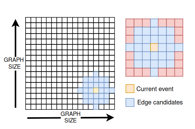
Figure 6: Context analysis and edge generation method. The context is stored in a SIZE $\times$ SIZE memory. For each incoming vertex (highlighted in orange), 29 edge candidates (blue) are read out. For each of these, a semi-sphere condition is checked and the final edges are generated.

The graph generation module is based on a two-port BRAM, which stores information about the last recorded events for each coordinate $x$ and $y$. The depth of the memory thus corresponds to all possible vertex positions (SIZE $\times$ SIZE, for N-Cars – 16 384). For each incoming event, a context containing information about the edge candidates (as shown in Figure 6) is read from the memory. Each memory cell stores the timestamp value of the last recorded event (7 bits for N-Cars), its polarity (1 bit) and the is_empty flag (1 bit) necessary to distinguish events with polarity equal to 0 and normalised time of occurrence equal to 0 from empty memory cells. Addressing the memory with vertex coordinates (ADDR = Y $\times$ SIZE + X) eliminates the need for storing the event $x$ and $y$ coordinates and thus simplifies the system implementation.

IX-C u_feature_map memory

In the synchronous part of the system, between consecutive convolutional layers, and between MaxPool layers and consecutive convolutional layers, a u_feature_map module is instantiated.

Inside the module there are three independent dual-port memories, which can be implemented using URAM or BRAM. Each memory has one read port and one read-write port. We exploit memory sharing – layers preceding the u_feature_map module write data to one of the memory blocks, and subsequent layers read the stored data (and perform zeroing of data no longer used in the system). A functional description of the module can be found in the publication. Switching and accessing the memories is controlled by a pointer that determines which layer is using which memory at a given moment.

Subsequent convolution layers use information about a vertex ($x$, $y$, and $t$), its feature map determined in previous convolution, and the feature maps of vertices connected to it by an edge to perform the calculations. Due to the fact that each memory is SIZE $\times$ SIZE, there is no need to store the $x$ and $y$ coordinates of the vertex (we use them to determine the address of the memory cell). In addition, because the entire ‘temporal channel’ of the graph is processed at once, there is no need to store $t$ values (only relative values between vertices connected by an edge are needed for the convolution). As a consequence, the width of each memory is (FEATURE_DIM $\times$ 8) + 18, where FEATURE_DIM is the width of the feature map. Its values are 8-bit, and an additional 18 bits are used to store information related to all edges.

IX-D Weights memory

To perform the convolutions, we need the values of the weights and biases determined in the training process. They are constant for a given network and stored in two ways. In the asynchronous part, due to the relatively small size of the weight matrices and the implementation of parallel multiplications, they are stored in distributed RAM. In the synchronous part, we use a single-port ROM (Read Only Memory) realised in BRAM. The depth of the memory used depends on the number of sequential multiplications, and its width on the size of the input feature map. Weights are stored as unsigned 8-bit values, and biases are stored as signed 32-bit values.

For example, in the EFGCN model, the first synchronous convolution implements multiplications in 32 steps. The input feature vector has 19 elements. The BRAM used to store the weights in this layer therefore has a depth of 32 and a width of ($19\times 8$) $+32$. The memories in the implementation are initialised from a file storing the values of weights and biases.

X Multiplication module

The key hardware module that is the basis for graph convolution is the multiplication module. It is initialised for each convolution layer and implemented in such a way that the increasing size of the feature map does not cause timing problems. The matrix (or vector for relaxed convolution) multiplication is implemented using LUT resources (due to the low precision of the multiplied values).

Important at this stage, however, is the quantisation of the values. Both the feature vectors and the weight matrices in the system are stored as unsigned 8-bit values. Before the multiplication, they must be rescaled. The implemented system uses three different scaling methods, tailored to specific data.

For weights, we simply subtract the layer-specific parameter ZERO_POINT_WEIGHTS (unsigned 8-bit, software-computed zero point for weights quantisation). In this way, before the multiplication operation, the weights are scaled to signed 9-bit values.

The features, on the other hand, are scaled in the software model using the floating-point scaling value. For their hardware quantisation, we use the fact that successive feature maps consist of the vectors determined in the previous convolutions and three additional values: the difference in $x$, $y$ and $t$ coordinates between the vertices connected by edges. These values before the first MaxPool layer reach permitted integer values in the range from $-3$ to $3$ (limited by the radius $R$), and in the synchronous part of the system from $-1$ to $1$. To implement quantisation for the FPGA, the vertex position difference values are read from the layer-specific look-up table array. Consequently, there is no need to multiply their values by a scalar.

Finally, the data after multiplication must also be scaled. The result of the multiplication is stored as signed 32-bit and bias values of the same precision are added to it. Due to the large possible range of values, the use of the LUTs is not possible at this stage. Instead, the result is multiplied by the layer-specific parameter MULTIPLIER_OUT (unsigned 32-bit) and divided by $2^{32}$. This operation corresponds to multiplying by a floating-point scale with values in the range $[0,1]$ (with an error considered to be insignificant). The scaling of the output values has been implemented using DSP multipliers and the division implemented as a simple bit shift. The final element of the scaling is the addition of the ZERO_POINT_OUT parameter value (unsigned 8-bit, software-computed zero point for output quantisation). After scaling, the feature map contains the values of unsigned 8-bit.

XI Scalability calculations

TABLE VI: Scalability calculations of the graph neural networks acceleration for different input graph sizes and TIME_WINDOW values.

Parameter	N-Cars	N-Caltech101
TIME_WINDOW	100 ms	50 ms
Graph SIZE	128	256
SIZE after MaxPool1	32	64
CONV2 & CONV3 throughput	625 000 ticks	156 250 ticks
Max CONV2 & CONV3 seq. mul.	64	4
SIZE after MaxPool2	16	32
CONV5 & CONV4 throughput	1 250 000 ticks	312 500 ticks
Max CONV4 & CONV5 seq. mul.	512	32

This section describes a method of estimating resource consumption for larger network models. The motivations and results of the calculations are described in the publication.

XI-A Impact of input graph size and TIME_WINDOW

TABLE VII: Estimation of resource utilisation on ZCU104 platform for EFGCN model for N-Caltech101 dataset. For module u_feature_mem2, an UltraRAM resource was used instead of BlockRAM because of the width and depth easily aligned to the UltraRAM interface.

Module	Feature map	Graph size	Sequential Muls	DSP usage	Memory WIDTH	Memory DEPTH	UltraRAM	BlockRAM
Total utilisation (sum)	-	-	-	184	-	-	24	202
Total utilisation (usage)	-	-	-	11%	-	-	25%	65%
u_gen_graph	-	256	-	-	-	-	-	19
u_async_conv1	16	256	1	64	-	-	-	-
u_maxpool1	-	-	-	-	-	-	-	-
u_feature_mem1	16	64	-	-	146	4096	-	49.5
u_sync_conv2	32	64	4	48	-	-	-	2.5
u_feature_mem2	32	64	-	-	274	4096	24	-
u_sync_conv3	32	64	4	48	-	-	-	4.5
u_maxpool2	-	-	-	-	-	-	-	-
u_feature_mem3	32	32	-	-	274	1024	-	24
u_sync_conv4	64	32	32	12	-	-	-	4.5
u_feature_mem4	64	32	-	-	530	1024	-	45
u_sync_conv5	64	32	32	12	-	-	-	8
u_maxpool3	-	-	-	-	-	-	-	-
u_feature_mem5	64	4	-	-	530	16	-	45

First of all, it is important to note that as the size of the input graph grows, the SIZE value for the entire system also expands, consequently demanding greater memory resources (each of the u_feature_map modules has correspondingly larger depths). However, it should be noted that the memory has been implemented in such a way that the user can choose whether it is implemented using BlockRAM or UltraRAM memory blocks. The decision should be made after analysing the whole model and taking into account the platform used and the available memory resources.

However, adaptation of the proposed model for a set with other hyperparameters additionally requires a re-analysis of the throughput for sequential convolutions. The relevant calculations are presented in Table VI. The required throughput for each convolution can be determined from TIME_WINDOW and SIZE based on the following formula:

$$throughput=\frac{TIME\_WINDOW}{SIZE\cdot NS\_PER\_CLK}$$ (12)

where SIZE denotes the current size of the graph after the MaxPool layer, and NS_PER_CLK is the time interval between successive clock rising edges expressed in nanoseconds. The throughput value represents the number of clock ticks that MaxPool needs to prepare the next ‘temporal channel’. The following convolution layers can use this time to determine the multiplication results. To determine the maximum number of multiplication operations that can be performed sequentially, the following formula can be used:

$$Max\_Seq\_Mul=\frac{2\cdot throughput}{SIZE\cdot SIZE\cdot EGDE\_NUM}$$ (13)

where Max_Seq_Mul denotes the maximum number of sequential multiplication operations and EDGE_NUM is the number of possible neighbours. The throughput has been multiplied by 2 due to the default use of two parallel multipliers (for the currently processed ‘temporal channel’ and for the previous one).

In the case of the EFGCN model for N-Cars classification, for each synchronous convolution it was possible to determine each element of the output feature map in a sequential manner. For N-Caltech101 dataset, however, this is not possible. For the CONV2 and CONV3 convolutions (output feature map size – 32), it is necessary to use 8 multiplication modules in parallel (the maximum number of possible sequential multiplications is now 4, as shown in Table VI). Consequently, the consumption of the DSP multipliers would increase by a factor of 8 (and the amount of logic resources used would increase proportionally). After another MaxPool layer, the throughput requirements are relaxed – 2 multiplication modules are needed in parallel (and the number of DSP multipliers doubles). The estimation of total resource utilisation for the EFGCN model used for classification for N-Caltech101 (where time window is 50 ms and input graph size is 256) is shown in Table VII.

XI-B Impact of additional layers

TABLE VIII: Estimation of resource utilisation on ZCU104 platform for model inspired by [24]. For simplicity of notation, the u_feature_mem layers have been included in the resources required for the corresponding convolution layer or MaxPool.

Module	Feature map	Graph size	Sequential Muls	DSP usage	Memory WIDTH	Memory DEPTH	UltraRAM	BlockRAM
Total utilisation (sum)	-	-	-	294	-	-	91	290
Total utilisation (usage)	-	-	-	17%	-	-	94%	93%
u_gen_graph	-	256	-	-	-	-	-	19
(async) CONV1	8	256	1	32	-	-	-	-
(async) CONV2	16	256	1	64	64	65536	17	-
MaxPool 4x4	16	64	-	-	146	4096	18	-
(sync) CONV3	32	64	4	48	274	4096	24	2.5
(sync) CONV4	32	64	4	48	274	4096	24	4.5
(sync) CONV5	32	64	4	48	-	-	-	4.5
MaxPool 2x2	32	32	-	-	274	1024	-	24
(sync) CONV6	64	32	32	12	530	1024	-	49.5
(sync) CONV7	64	32	32	12	530	1024	-	53
(sync) CONV8	64	32	32	12	-	-	-	8
MaxPool 2x2	64	16	-	-	530	768	8	-
(sync) CONV9	128	16	256	6	1042	768	-	37
(sync) CONV10	128	16	256	6	1042	768	-	44
(sync) CONV11	128	16	256	6	-	-	-	15
MaxPool 4x4	128	4	-	-	1042	48	-	29

TABLE IX: Estimation of resource utilisation on ZCU104 platform for model inspired by [19].

Module	Feature map	Graph size	Sequential Muls	DSP usage	Memory WIDTH	Memory DEPTH	UltraRAM	BlockRAM
Total utilisation (sum)	-	-	-	368	-	-	82	292.5
Total utilisation (usage)	-	-	-	21%	-	-	85%	94%
u_gen_graph	-	256	-	-	-	-	-	19
(async) CONV1	16	256	1	64	-	-	-	-
(async) CONV2	16	256	1	64	128	65536	34	-
MaxPool 4x4	16	64	-	-	146	4096	-	49.5
(sync) CONV3	64	64	4	96	530	4096	48	3
(sync) CONV4	64	64	4	96	-	-	-	8
MaxPool 2x2	64	32	-	-	530	1024	-	45
(sync) CONV5	64	32	32	12	530	1024	-	53
(sync) CONV6	64	32	32	12	-	-	-	8
MaxPool 2x2	64	16	-	-	530	768	-	15
(sync) CONV7	64	16	256	6	530	768	-	23
(sync) CONV8	64	16	256	6	-	-	-	8
MaxPool 2x2	64	8	-	-	530	192	-	15
(sync) CONV9	64	8	1024	6	530	192	-	23
(sync) CONV10	64	8	1024	6	530	192	-	23

Another form of scaling the solution to consider is to change the architecture of the network model and increase the number of convolutional layers (in order to improve the accuracy of the model). Based on an analysis of the utilisation of the model implemented for the SoC FPGA (for the N-Cars dataset), the following conclusions can be drawn. Each successive MaxPool layer significantly reduces the required memory depth necessary to store the feature maps. At the same time, the memory width is affected by the size of the convolution output (the more feature map elements, the more memory required). The number of possible sequential multiplications, on the other hand, affects the utilisation of the DSP multipliers.

Moreover, in the EFGCN model we use only one asynchronous convolution. If further convolution layers are added before the MaxPool module, the operations are performed in an analogous way. However, it should be emphasised that only for the first layer all the information needed for the convolution is in the input data (subsequent layers use the features determined by the previous layers). For further convolutions, a BlockRAM with dimensions SIZE $\times$ SIZE is required, which stores the feature maps for all recently recorded events for the given coordinates ($x$, $y$) (the order of events is preserved, so in the memory we have an access to the feature map of all vertices connected by an edge to the currently processed one).

When designing the network architecture, these considerations should be taken into account and the size of the network should be a compromise between performance requirements and the resources available on the hardware. As a reference, an estimation of memory utilisation was carried out for the model inspired by work [24], where PointNet++ was first used for object detection and classification of event data. The model uses 11 convolution layers and 4 MaxPool layers. We use an additional method of memory optimisation during the calculation: each MaxPool relaxes the bandwidth requirements. For further convolutional layers in this model, the number of allowed sequential multiplications doubles the number of output feature map elements. In this situation, reading data from two memories simultaneously is not necessary. Consequently, the module u_feature_mem, instead of three two-port memories, can use only one two-port memory (with three times the depth), where one of the ports is used by the previous layer and the other by the next layer. Using this method, the memory resources used by further layers can be significantly reduced. The results of the memory utilisation estimation for a model with significantly more layers are shown in Table VIII. Both memories used for feature maps and weights and DSP modules are included. For the calculations we assume the classification for N-Caltech101, i.e. a time window of 50 ms and a graph size of 256. Such a network requires 93% and 94% of BlockRAM and UltraRAM resources, respectively. It can therefore be assumed that this is the maximum model that can be implemented using the described accelerator for a medium-sized FPGA chip available on the ZCU104 board.

Implementation of larger models would require the use of external memory resources (DDR4 available both for PL and PS on ZCU104 board). These resources have significantly higher capacity and high bandwidth. However, they are characterised by variable latency and their efficient use, that would not significantly affect system throughput, requires a number of addressing and scheduling techniques. Evaluation for the use of external memory for significantly larger models is a part of planned future work. However, it is worth noting that other works rarely apply larger graph network models to event data. For example, work [19] established the state-of-the-art accuracy for object detection on event data with a graph network using 10 convolutional layers and 4 MaxPool layers. Furthermore, this work uses graph edges limited to 16 and feature maps with a maximum size of 64 (for Baseline, 128 for Large), making it a suitable solution for the accelerator we have designed. Table IX shows the resource consumption estimates for the model inspired by this method. Skip connections used are not included here, not being supported yet by the designed accelerator. The inclusion of such connections is also a part of planned future work.

Another strategy for implementing larger models is to optimise memory use in proposed hardware module. Particularly for last convolutional layers, memories have wide input interfaces and small depths, leading to high memory consumption. As part of future work, we plan to investigate the possibility of reading data using a clock with a higher frequency, thus decreasing memory consumption.

In summary, the applied method allows scalability for larger models and higher resolutions, which makes the presented solution a good starting point for further research on real-time embedded object recognition on continuous stream of event data. Despite the relatively low accuracy results for the EFGCN model, the above scalability calculations allow us to conclude that the full accelerator potential for the medium-sized SoC FPGA like XCZU7EV available on the ZCU104 board has not been fully utilised and larger models can be implemented.

References

- [1] F. K. Konstantinidis, S. G. Mouroutsos, and A. Gasteratos, “The role of machine vision in industry 4.0: an automotive manufacturing perspective,” in 2021 IEEE International Conference on Imaging Systems and Techniques (IST), 2021, pp. 1–6.
- [2] L. Bodenhagen, A. R. Fugl, A. Jordt, M. Willatzen, K. A. Andersen, M. M. Olsen, R. Koch, H. G. Petersen, and N. Krüger, “An adaptable robot vision system performing manipulation actions with flexible objects,” IEEE transactions on automation science and engineering, vol. 11, no. 3, pp. 749–765, 2014.
- [3] T.-H. Pham, A. Kheddar, A. Qammaz, and A. A. Argyros, “Towards force sensing from vision: Observing hand-object interactions to infer manipulation forces,” in Proceedings of the IEEE conference on computer vision and pattern recognition, 2015, pp. 2810–2819.
- [4] P. Lichtsteiner, C. Posch, and T. Delbruck, “A 128 128 120 db 15 s latency asynchronous temporal contrast vision sensor,” IEEE Journal of Solid-State Circuits, vol. 43, no. 2, pp. 566–576, 2008.
- [5] G. Gallego, T. Delbrück, G. Orchard, C. Bartolozzi, B. Taba, A. Censi, S. Leutenegger, A. J. Davison, J. Conradt, K. Daniilidis, et al., “Event-based vision: A survey,” IEEE transactions on pattern analysis and machine intelligence, vol. 44, no. 1, pp. 154–180, 2020.
- [6] S. Afshar, N. Ralph, Y. Xu, J. Tapson, A. v. Schaik, and G. Cohen, “Event-based feature extraction using adaptive selection thresholds,” Sensors, vol. 20, no. 6, p. 1600, 2020.
- [7] R. Ghosh, A. Mishra, G. Orchard, and N. V. Thakor, “Real-time object recognition and orientation estimation using an event-based camera and cnn,” in 2014 IEEE Biomedical Circuits and Systems Conference (BioCAS) Proceedings, 2014, pp. 544–547.
- [8] E. Perot, P. De Tournemire, D. Nitti, J. Masci, and A. Sironi, “Learning to detect objects with a 1 megapixel event camera,” Advances in Neural Information Processing Systems, vol. 33, pp. 16 639–16 652, 2020.
- [9] Z. Chen, J. Wu, J. Hou, L. Li, W. Dong, and G. Shi, “Ecsnet: Spatio-temporal feature learning for event camera,” IEEE Transactions on Circuits and Systems for Video Technology, vol. 33, no. 2, pp. 701–712, 2022.
- [10] N. Messikommer, D. Gehrig, A. Loquercio, and D. Scaramuzza, “Event-based asynchronous sparse convolutional networks,” in Computer Vision–ECCV 2020: 16th European Conference, Glasgow, UK, August 23–28, 2020, Proceedings, Part VIII 16. Springer, 2020, pp. 415–431.
- [11] M. Gehrig, S. B. Shrestha, D. Mouritzen, and D. Scaramuzza, “Event-based angular velocity regression with spiking networks,” in 2020 IEEE International Conference on Robotics and Automation (ICRA). IEEE, 2020, pp. 4195–4202.
- [12] L. Cordone, B. Miramond, and S. Ferrante, “Learning from event cameras with sparse spiking convolutional neural networks,” in 2021 International Joint Conference on Neural Networks (IJCNN). IEEE, 2021, pp. 1–8.
- [13] Z. Liu, J. Wu, G. Shi, W. Yang, W. Dong, and Q. Zhao, “Motion-oriented hybrid spiking neural networks for event-based motion deblurring,” IEEE Transactions on Circuits and Systems for Video Technology, 2023.
- [14] Q. Wang, Y. Zhang, J. Yuan, and Y. Lu, “Space-time event clouds for gesture recognition: From rgb cameras to event cameras,” in 2019 IEEE Winter Conference on Applications of Computer Vision (WACV), 2019, pp. 1826–1835.
- [15] Y. Bi, A. Chadha, A. Abbas, E. Bourtsoulatze, and Y. Andreopoulos, “Graph-based object classification for neuromorphic vision sensing,” in Proceedings of the IEEE/CVF international conference on computer vision, 2019, pp. 491–501.
- [16] A. Mitrokhin, Z. Hua, C. Fermüller, and Y. Aloimonos, “Learning visual motion segmentation using event surfaces,” in 2020 IEEE/CVF Conference on Computer Vision and Pattern Recognition (CVPR), 2020, pp. 14 402–14 411.
- [17] Y. Li, H. Zhou, B. Yang, Y. Zhang, Z. Cui, H. Bao, and G. Zhang, “Graph-based asynchronous event processing for rapid object recognition,” in Proceedings of the IEEE/CVF International Conference on Computer Vision, 2021, pp. 934–943.
- [18] S. Schaefer, D. Gehrig, and D. Scaramuzza, “Aegnn: Asynchronous event-based graph neural networks,” in Proceedings of the IEEE/CVF conference on computer vision and pattern recognition, 2022, pp. 12 371–12 381.
- [19] D. Gehrig and D. Scaramuzza, “Pushing the limits of asynchronous graph-based object detection with event cameras,” arXiv preprint arXiv:2211.12324, 2022.
- [20] M. Liu and T. Delbruck, “Edflow: Event driven optical flow camera with keypoint detection and adaptive block matching,” IEEE Transactions on Circuits and Systems for Video Technology, vol. 32, no. 9, pp. 5776–5789, 2022.
- [21] Y. Gao, B. Zhang, Y. Ding, and H. K.-H. So, “A composable dynamic sparse dataflow architecture for efficient event-based vision processing on fpga,” in Proceedings of the 2024 ACM/SIGDA International Symposium on Field Programmable Gate Arrays, 2024, pp. 246–257.
- [22] Z. Wu, S. Pan, F. Chen, G. Long, C. Zhang, and S. Y. Philip, “A comprehensive survey on graph neural networks,” IEEE transactions on neural networks and learning systems, vol. 32, no. 1, pp. 4–24, 2020.
- [23] Y. Sekikawa, K. Hara, and H. Saito, “Eventnet: Asynchronous recursive event processing,” in Proceedings of the IEEE/CVF conference on computer vision and pattern recognition, 2019, pp. 3887–3896.
- [24] K. Jeziorek, A. Pinna, and T. Kryjak, “Memory-efficient graph convolutional networks for object classification and detection with event cameras,” in 2023 Signal Processing: Algorithms, Architectures, Arrangements, and Applications (SPA), 2023, pp. 160–165.
- [25] C. R. Qi, H. Su, K. Mo, and L. J. Guibas, “Pointnet: Deep learning on point sets for 3d classification and segmentation,” in Proceedings of the IEEE conference on computer vision and pattern recognition, 2017, pp. 652–660.
- [26] C. R. Qi, L. Yi, H. Su, and L. J. Guibas, “Pointnet++: Deep hierarchical feature learning on point sets in a metric space,” Advances in neural information processing systems, vol. 30, 2017.
- [27] S. Hochreiter and J. Schmidhuber, “Long short-term memory,” Neural Comput., vol. 9, no. 8, p. 1735–1780, nov 1997. [Online]. Available: https://doi.org/10.1162/neco.1997.9.8.1735
- [28] M. Fey, J. E. Lenssen, F. Weichert, and H. Müller, “Splinecnn: Fast geometric deep learning with continuous b-spline kernels,” in Proceedings of the IEEE conference on computer vision and pattern recognition, 2018, pp. 869–877.
- [29] C. Morris, M. Ritzert, M. Fey, W. L. Hamilton, J. E. Lenssen, G. Rattan, and M. Grohe, “Weisfeiler and leman go neural: Higher-order graph neural networks,” in Proceedings of the AAAI conference on artificial intelligence, vol. 33, no. 01, 2019, pp. 4602–4609.
- [30] K. Jeziorek, P. Wzorek, K. Blachut, A. Pinna, and T. Kryjak, “Optimising graph representation for hardware implementation of graph convolutional networks for event-based vision,” arXiv preprint arXiv:2401.04988, 2024.
- [31] B. Zhang, H. Zeng, and V. Prasanna, “Hardware acceleration of large scale gcn inference,” in 2020 IEEE 31st International Conference on Application-specific Systems, Architectures and Processors (ASAP). IEEE, 2020, pp. 61–68.
- [32] Z. Tao, C. Wu, Y. Liang, K. Wang, and L. He, “Lw-gcn: A lightweight fpga-based graph convolutional network accelerator,” ACM Transactions on Reconfigurable Technology and Systems, vol. 16, no. 1, pp. 1–19, 2022.
- [33] Z. Wang, Z. Que, W. Luk, and H. Fan, “Customizable fpga-based accelerator for binarized graph neural networks,” in 2022 IEEE International Symposium on Circuits and Systems (ISCAS), 2022, pp. 1968–1972.
- [34] H. Zhou, B. Zhang, R. Kannan, V. Prasanna, and C. Busart, “Model-architecture co-design for high performance temporal gnn inference on fpga,” in 2022 IEEE International Parallel and Distributed Processing Symposium (IPDPS), 2022, pp. 1108–1117.
- [35] J.-F. Zhang and Z. Zhang, “Point-x: A spatial-locality-aware architecture for energy-efficient graph-based point-cloud deep learning,” in MICRO-54: 54th Annual IEEE/ACM International Symposium on Microarchitecture, 2021, pp. 1078–1090.
- [36] Z. Zhang and H. Li, “Fpga implementation of a point cloud processing knn algorithm used in gcn network,” in 2023 5th International Conference on Electronics and Communication Technologies (ECT, 2023, pp. 119–123.
- [37] Y. Li, Y. Zhang, and R. Lai, “Tinypillarnet: Tiny pillar-based network for 3d point cloud object detection at edge,” IEEE Transactions on Circuits and Systems for Video Technology, 2023.
- [38] L. Bai, Y. Lyu, X. Xu, and X. Huang, “Pointnet on fpga for real-time lidar point cloud processing,” in 2020 IEEE International Symposium on Circuits and Systems (ISCAS). IEEE, 2020, pp. 1–5.
- [39] K. Sugiura and H. Matsutani, “P3net: Pointnet-based path planning on fpga,” in 2022 International Conference on Field-Programmable Technology (ICFPT). IEEE, 2022, pp. 1–9.
- [40] M. Fey and J. E. Lenssen, “Fast graph representation learning with PyTorch Geometric,” in ICLR Workshop on Representation Learning on Graphs and Manifolds, 2019.
- [41] B. Jacob, S. Kligys, B. Chen, M. Zhu, M. Tang, A. Howard, H. Adam, and D. Kalenichenko, “Quantization and training of neural networks for efficient integer-arithmetic-only inference,” in Proceedings of the IEEE conference on computer vision and pattern recognition, 2018, pp. 2704–2713.
- [42] A. Sironi, M. Brambilla, N. Bourdis, X. Lagorce, and R. Benosman, “Hats: Histograms of averaged time surfaces for robust event-based object classification,” in Proceedings of the IEEE conference on computer vision and pattern recognition, 2018, pp. 1731–1740.
- [43] G. Orchard, A. Jayawant, G. K. Cohen, and N. Thakor, “Converting static image datasets to spiking neuromorphic datasets using saccades,” Frontiers in neuroscience, vol. 9, p. 159859, 2015.
- [44] H. Li, H. Liu, X. Ji, G. Li, and L. Shi, “Cifar10-dvs: An event-stream dataset for object classification,” Frontiers in Neuroscience, vol. 11, 2017. [Online]. Available: https://www.frontiersin.org/journals/neuroscience/articles/10.3389/fnins.2017.00309
- [45] T. Serrano-Gotarredona and B. Linares-Barranco, “Poker-dvs and mnist-dvs. their history, how they were made, and other details,” Frontiers in Neuroscience, vol. 9, 2015. [Online]. Available: https://www.frontiersin.org/journals/neuroscience/articles/10.3389/fnins.2015.00481
- [46] Y. Deng, H. Chen, H. Liu, and Y. Li, “A voxel graph cnn for object classification with event cameras,” in Proceedings of the IEEE/CVF Conference on Computer Vision and Pattern Recognition, 2022, pp. 1172–1181.
- [47] B. Xie, Y. Deng, Z. Shao, H. Liu, and Y. Li, “Vmv-gcn: Volumetric multi-view based graph cnn for event stream classification,” IEEE Robotics and Automation Letters, vol. 7, no. 2, pp. 1976–1983, 2022.
- [48] D. Liu, T. Wang, and C. Sun, “Voxel-based multi-scale transformer network for event stream processing,” IEEE Transactions on Circuits and Systems for Video Technology, 2023.
- [49] I. Loshchilov and F. Hutter, “Decoupled weight decay regularization,” arXiv preprint arXiv:1711.05101, 2017.
- [50] G. Hinton, O. Vinyals, and J. Dean, “Distilling the knowledge in a neural network,” arXiv preprint arXiv:1503.02531, 2015.
- [51] K. Xu, L. Wang, J. Xin, S. Li, and B. Yin, “Learning from teacher’s failure: A reflective learning paradigm for knowledge distillation,” IEEE Transactions on Circuits and Systems for Video Technology, 2023.
- [52] K. Sugiura and H. Matsutani, “An efficient accelerator for deep learning-based point cloud registration on fpgas,” in 2023 31st Euromicro International Conference on Parallel, Distributed and Network-Based Processing (PDP), 2023, pp. 68–75.
- [53] B. Ramesh, A. Ussa, L. Della Vedova, H. Yang, and G. Orchard, “Low-power dynamic object detection and classification with freely moving event cameras,” Frontiers in neuroscience, vol. 14, p. 505328, 2020.