Experimental Modeling of Chiral Active Robots and a Minimal Model of Non-Gaussian Displacements

Abstract

We design 3D-printed motor-driven active particles and find that their dynamics can be characterized using the model of overdamped chiral active Brownian particles (ABPs), as demonstrated by measured angular statistics and translational mean squared displacements (MSDs). Furthermore, we propose a minimal model that reproduces the double-peak velocity distributions and further predicts a transition from the single-peak to the double-peak displacement distributions in short-time regimes. The model provides a clear physics picture of these phenomena, originating from the competition between the active motion and the translational diffusion. Our experiments confirm such picture. The minimal model enhances our understanding of activity-driven non-Gaussian phenomena. The designed particles could be further applied in the study of collective chiral motions.

I Introduction

Active matter consists of self-propelled units and exhibits novel non-equilibrium dynamics [1, 2, 3]. Examples range from biological entities, such as cells [4, 5], bacteria [6, 7], and animal collectives [8], to human-engineered systems, such as active colloids [9, 10], shaker-driven active grains [11, 12, 13, 14, 15, 16], and self-propelled robots [17, 18, 19, 20]. These systems exhibit rich non-equilibrium phenomena, including non-Gaussian diffusion [21, 15, 22, 23], active pressure [24, 25], motility-induced phase separation [26, 27, 28], self-alignments of active solids  [19], and as well as chirality induced phase separation [29] and odd viscosity [30, 31, 32, 33].

These phenomena could emerge from microscopic models [34, 35, 36, 37]. One of the most important models is that of active Brownian particles (ABPs), where a single particle moves along a given direction with constant speed, and the direction changes randomly due to rotational noise. The model is theoretically studied in [34, 38, 39, 40], experimentally realized in the microscopic systems of active colloidal particles[21, 26, 41], and in the macroscopic systems of shaker-driven active granular particles from overdamped dynamics [14] to underdamped dynamics [15, 16].

The experimental realizations above [14, 15, 16] are essentially achiral. For experimental studying of chiral ABPs (which, in addition to angular diffusion, exhibit fixed angular speeds), the diffusion of shaker-driven chiral grass seeds in lattices was studied in [42], where the diffusivity could be strongly affected by the lattices’ geometry. The collective motion of commercially available light-driven walkers was recently studied in [20]. The mean squared displacements (MSDs) of a single walker indicate the validity of the overdamped chiral ABPs. But direct statistics of the angular dynamics of are absent, which are key characteristics of chirality. To what extend can the model of chiral ABPs be applied to other macroscopic systems is still unknown. In addition, neither grass seeds nor light-driven walkers are easy to modify, so robust and modifiable chiral ABPs are still needed in experiments.

Meanwhile, in contrast to Maxwellian velocity distributions of Brownian particles, the velocities distributions of ABPs may exhibit double-peak profiles as shown in [21, 15]. Such non-Gaussian distributions were further studied in [23] based on the Fokker-Planck equation of underdamped chiral ABPs, in which inertia is crucial for the double-peak velocity distributions. However, this is probably not the whole story, as double-peak distributions have also been observed experimentally in active colloidal systems [21] and theoretically calculated by expanding the Smoluchowski equation in orientational moments of the model of overdamped ABPs [22]. In both cases, inertia is negligible. A clear physics picture of the double-peak velocities distributions is still missing.

In this paper, we design 3D-printed electric motor driven particles, which encode both persistent and rotational motion. We are interested in two aspects: first, the robustness of the model of chiral ABPs, i.e. to what extent can the model describe our 3D-printed electric active particles, especially, in terms of angular dynamics statistics and the MSDs; second, can a minimal model be constructed to describe the double-peak velocity distributions and further predict short-time displacement distributions?

The paper is organized as follows: we introduce the experimental setup in Sec. II and the model of overdamped chiral ABPs in Sec. III. Then we experimentally test the model by measuring the angular statistics in Sec. IV, and the MSDs in Sec. V. Furthermore, we propose a minimal model to explain the double-peak velocity distributions found in our experiments in Sec. VI and extend it to non-Gaussian displacements in Sec. VII. We conclude in Sec. VIII.

II Experimental setup

We design 3D-printed, vibration motor driven active particles, see Fig. 1. The particles are different in weights. The heavy particle has a weight of 31.2g with four button batteries connected in parallel, see Fig. 1 (a). The light particle has a weight of 18.1g with one button battery only, see Fig. 1 (b).

The shells of the particles are 3D-printed with ABS thermosetting resin. Each particle is cylinder covered by a circular disc cover with a diameter of 40mm. At the bottom of each particle, four straight cylindrical legs are arranged in a square, two diagonal ones are on the same straight line with the long axis of a vibration motor inside, see Fig. 1 (a) and (b). A photo of the heavy particle is displayed in Fig. 1 (c).

The detailed driven mechanism of our active particles is out of scope of this paper due to its complexity of non-linear dynamics [43, 44], which is essentially the centrifugal motion of the vibration motor causing two modes of motion, as shown in Fig. 1 (d). The vertical vibration with weight asymmetry enables the particles to behave as self-propelled polar ”walkers” [11, 45], while the horizontal vibration induces a torque that makes the particles move in circles [46].

The positions and the angles of the active particles are captured by a camera operating at 60fps. A recorded trajectory of the heavy particle is shown in Fig. 1 (e).

Figure 1: Design of 3D-printed and motor driven active particles. (a-b) Structures of a heavy and a light particle. (c) A physical picture of a heavy particle. (d) Illustration of driven mechanism. (e) A trajectory recorded by a camera operating at 60fps.

III Model

We explore the dynamics of our motor-driven chiral particles by the model of overdamped chiral ABPs as follows

$$\bm{v} = v_{0}\bm{n}+\sqrt{2D_{T}}\bm{\xi}_{r},$$ (1a)

$$\dot{\theta} = \Omega+\sqrt{2D_{R}}\xi_{\theta}.$$ (1b)

The total velocity $\bm{v}$ comprises both the self-propelled velocity and the effective thermal velocity induced by translational noise, where $v_{0}$ is the strength of the self-propelled velocity, $\bm{n}=(\cos\theta,\sin\theta)$ is its direction, $D_{T}$ is the translational diffusivity, $\bm{\xi}_{r}=(\xi_{x},\xi_{y})$ is Gaussian white noise with zero mean and variance $\langle\xi_{\alpha}(t)\xi_{\beta}(t^{\prime})\rangle=\delta_{\alpha,\beta}\delta(t-t^{\prime}),\,\alpha,\beta\in\{x,y\}$. The total angular speed $\dot{\theta}$ comprises both the fixed angular speed $\Omega$ and the rotational noise, where $D_{R}$ is the rotational diffusivity, $\xi_{\theta}$ is Gaussian white noise with zero mean and variance $\langle\xi_{\theta}(t)\xi_{\theta}(t^{\prime})\rangle=\delta(t-t^{\prime})$. The dynamics are completely characterized by these four parameters: $v_{0}$, $D_{T}$, $\Omega$ and $D_{R}$.

IV Angular statistics

Figure 2: Angular statistics of chiral particles. In the upper row are the results of the heavy particle, while in the lower, the results of the light one. (a) and (b) are the PDFs of the angular speed. Bars are experimental statistics. Solid black curves are normal distribution fitting. (c) and (d) are the noise ACFs. (e) and (f) are angular MSDs. Dotted points are experimental data. Solid orange lines are theoretical formula Eq. (2). (g) and (h) are ACFs of the directions. Dotted points with error bars are experimental data. Solid orange lines are theoretical formula Eq. (3).

The angular statistics of the two particles are plotted in Fig. 2. In the upper row are the results of the heavy particle, while in the lower are the results of the light one. The probability distribution functions (PDFs) of their angular speed $\dot{\theta}$, are normally distributed, indicating that the noise is Gaussian, see Fig. 2 (a) and (b). The time auto correlation functions (ACFs) of the noises decay to zeros in a few time intervals of $h$ ($h=1/60s$ representing the time interval between adjacent frames in the captured video), see Fig. 2 (c) and (d). In order to extract the fixed angular speed $\Omega$ and the rotational diffusivity $D_{R}$, we fit the mean $\langle\Delta\theta(t)\rangle=\Omega t$ and the variance $Var[\Delta\theta(t)]=2D_{R}t$ in short time, where $\Delta\theta(t):=\theta(t)-\theta(0)$ is the angular displacement. In practice, we fits the mean and the variance in the time interval $t=100h$. The extracted $\Omega$ and $D_{R}$ for both heavy and light particles are recorded in Table 1.

To further check the accuracy of the extracted $\Omega$ and $D_{R}$, we compute the MSD of the angle $\theta(t)$ and the ACF of the direction $\bm{n}(t)$ from the model of overdamped chiral ABPs, and compare them with the direct measurements.

Eq. (1b) indicates the MSD of the angle should be

$$MSD_{\theta}(t)=\Big{\langle}\Delta\theta(t)^{2}\Big{\rangle}=\Omega^{2}t^{2}+2D_{R}t,$$ (2)

where we use the non-correlation of the noise $\langle\xi_{\theta}(t)\xi_{\theta}(t^{\prime})\rangle=\delta(t-t^{\prime})$. The MSDs of the angles can be well fitted by the theoretical formula Eq. (2), where the dotted points are experimental data and the solid orange lines are the predictions from Eq. (2) with measured $\Omega$ and $D_{R}$ in Table 1, see Fig. 2 (e) and (f). Note that in short time regimes, the angular MSD of the heavy particle is already in the linear regime, due to the domination of the angular diffusion term $2D_{R}t$. While in long time regimes, the angular MSDs of both particles are proportional to $t^{2}$, due to the domination of the fixed rotation term $\Omega^{2}t^{2}$.

According to Eq. (1b), we compute the ACF of the direction $\bm{n}(t)$

$$\Big{\langle}\bm{n}(t)\cdot\bm{n}(0)\Big{\rangle}=\Big{\langle}\cos\Delta\theta(t)\Big{\rangle}=e^{-D_{R}t}\cos\Omega t,$$ (3)

where we have used the property that $\Delta\theta(t)$ is normally distributed with mean $\mu=\Omega t$ and variance $\sigma^{2}=2D_{R}t$. The ACFs of the directions for both heavy and light particles can be reasonably fitted by Eq. (3). The small deviation may arise from fluctuations in $D_{R}$ and $\Omega$ due to the inevitable battery power instability.

V Mean squared displacements

The complete model of chiral ABPs requires the additional parameters: the self-propelled velocity $v_{0}$ and the translational diffusivity $D_{T}$, which are extracted from the PDFs of the particles’ velocities being parallel to the angular direction, $f_{v_{\parallel}}(v)$. The PDFs for both two particles are found to be Gaussian, and the self-propelled velocities equal to the means, $v_{0}=\mu_{v_{\parallel}}$. The translational diffusivities relate to the variances as $D_{T}=2\sigma^{2}_{v_{\parallel}}h$. We collect all the parameters for both particles in Table 1.

Table 1: Parameters of chiral particles.

	$\Omega\,[rad/s]$	$D_{R}\,[rad^{2}/s]$	$v_{0}\,[cm/s]$	$D_{T}\,[cm^{2}/s]$
heavy	0.457$\pm$0.068	0.0134 $\pm$0.0056	1.04$\pm$0.10	0.007$\pm$0.001
light	3.591$\pm$0.466	0.220$\pm$0.092	8.70$\pm$0.29	0.037$\pm$0.009

The translational MSD of a chiral ABP in  Eq. (1) can be calculated analytically [47, 48, 49],

$$\langle|\mathbf{r}(t)-\mathbf{r}(0)|^{2}\rangle=\frac{2\left(\frac{v_{0}}{D_{R}}\right)^{2}}{1+\Gamma^{2}}\Big{\{}-\frac{1-\Gamma^{2}}{1+\Gamma^{2}}+D_{R}t+$$ (4)

$$e^{-D_{R}t}\big{[}\frac{1-\Gamma^{2}}{1+\Gamma^{2}}\cos(\Gamma D_{R}t)-\frac{2\Gamma}{1+\Gamma^{2}}\sin(\Gamma D_{R}t)\big{]}\Big{\}}+4D_{T}t,$$

where $\Gamma=\Omega/D_{R}$ represents the strength of the chirality ($\Gamma=0$, achirality). In long time regimes, the chiral ABP behaves diffusively with diffusivity

$$D_{eff}=\lim_{{t\to\infty}}\frac{\langle|\mathbf{r}(t)-\mathbf{r}(0)|^{2}\rangle}{4t}=\frac{v_{0}^{2}}{2D_{R}(1+\Gamma^{2})}+D_{T},$$ (5)

while in short time regimes, the particle dynamics shifts from diffusion $D_{T}t$ to ballistic motion $v_{0}^{2}t^{2}$.

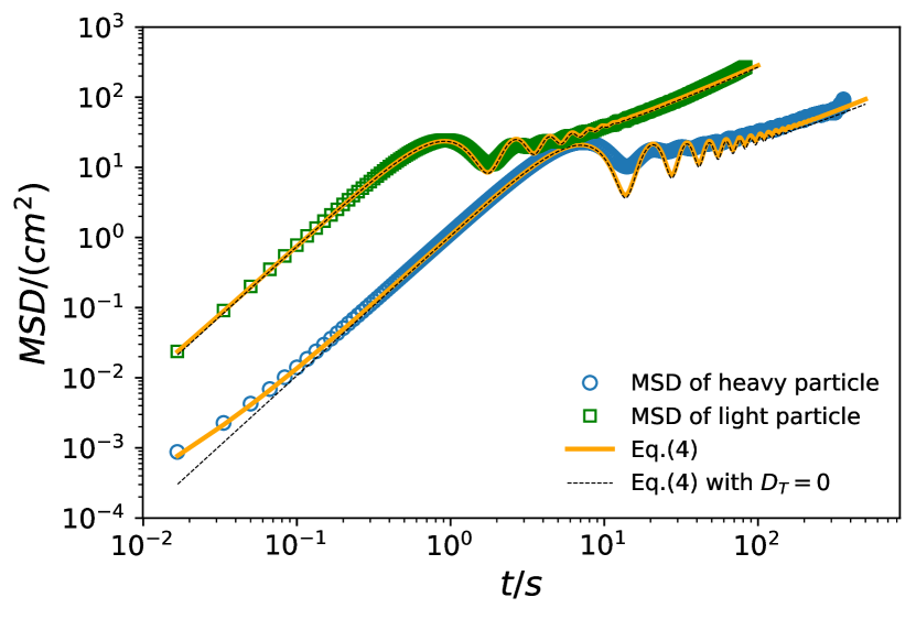
Figure 3: MSDs of heave and light particles. The solid orange lines are the results from Eq. (4) with input values of $v_{0},\Omega,D_{R},D_{T}$ in Table 1. The dashed black lines are the results from Eq. (4) with the same input values except for $D_{T}=0$.

The experimental results of the translational MSDs of both heavy and light particles match the analytical expression Eq. (4) well, including the crossover from diffusion $D_{T}t$ to ballistic motion $v_{0}^{2}t^{2}$, see Fig. 3, which supports the validity of the model of overdamped chiral ABPs for our experimental particles. Importantly, all the parameters input to Eq. (4) are directly from Table 1 without any fitting.

VI Velocity distributions in laboratory coordinates

Let’s consider the velocity distributions along an arbitrary direction in the laboratory coordinates. The velocity distributions are typically non-Gaussian. They may exhibit double-peak, which was found in [21, 15] and further treated as the inertial effect by Fokker-Planck equation of a single underdamped chiral ABP [23]. Note that the double-peak distributions found in [21] are of active colloids, whose dynamics are typically overdamped, suggesting that inertial is probably not the crucial point for the double-peak distributions.

Based on the model of overdamped chiral ABPs, we construct a minimal model, which predicts a double-peak velocity distribution arising from the domination of the active velocity over the effective thermal velocity due to translational noise. The prediction is confirmed by the experimental results.

VI.1 Minimal model

The velocity along x-axis in Eq. (1a) is the sum of two independent components $v_{x}=v_{A}+v_{T}$; the active velocity $v_{A}=v_{0}\cos\theta$ and the effective thermal velocity $v_{T}=\sqrt{2D_{T}}\xi_{x}$. The PDF of the total velocity $f_{v_{x}}$ should be the convolution of the PDFs of the two independent components

$$f_{v_{x}}(v)=\int^{\infty}_{-\infty}f_{v_{A}}(v^{\prime})f_{v_{T}}(v-v^{\prime})dv^{\prime}.$$ (6)

The PDF of the effective thermal velocity should be of normal distribution as

$$f_{v_{T}}(v)=\mathcal{N}(0,2D_{T}/h),$$ (7)

due to the white Gaussian noise property $\xi_{x}=\frac{dW_{t}}{dt}\approx\frac{W_{t+h}-W_{t}}{h}\sim\mathcal{N}(0,1/h)$. $h$ is the time resolution in experiment. $W_{t}$ is a standard Wiener process [50] with vanished initial value $W_{0}=0$ and independent and normal distributed increment $W_{t_{1}}-W_{t_{0}}\sim\mathcal{N}(0,t_{1}-t_{0})$ for any $t_{1}>t_{0}\geq 0$.

Let’s consider the PDF of the active velocity $f_{v_{A}}$. Due to the angular diffusion $\sqrt{2D_{R}}\xi_{\theta}$ and fixed orientation speed $\Omega$, the angle should be uniformly distributed, $\theta\sim$ uniform $(0,2\pi)$. The corresponding PDF of $\cos\theta$ is $f_{\cos\theta}(x)=\frac{1}{\pi\sqrt{1-x^{2}}},for\,x\in[-1,1];=0,\,else.$ Thus the PDF of the active velocity $v_{A}=v_{0}\cos\theta$ should be

$$f_{v_{A}}(v)=\begin{cases}\frac{1}{v_{0}\pi\sqrt{1-(v/v_{0})^{2}}},\quad&v\in[-v_{0},v_{0}],\\ 0,\quad&else.\end{cases}$$ (8)

Inserting Eq. (7) and Eq. (8) into Eq. (6), we get

$$f_{v_{x}}(v)=\frac{1}{v_{0}}\int^{1}_{-1}\frac{1}{\pi\sqrt{1-u^{2}}}\frac{1}{\sqrt{2\pi}\sigma_{v}}e^{-\frac{(\frac{v}{v_{0}}-u)^{2}}{2\sigma_{v}^{2}}}du,$$ (9)

where we have denoted $v_{th}=\sqrt{\frac{2D_{T}}{h}}$ as the strength of the effective thermal velocity and

$$\sigma_{v}=\frac{v_{th}}{v_{0}}=\frac{\sqrt{2D_{T}/h}}{v_{0}}$$ (10)

as the ratio of the effective thermal velocity to the active velocity.

One can readily compare the numerical integrals of Eq. (9) with the experimental results. Before that, let’s discuss two limiting regimes to understand the distribution profiles.

• For $\sigma_{v}\gg 1$, the effective thermal velocity dominates over the active velocity.

  $$\begin{split}f_{v_{x}}(v)&=\frac{1}{v_{0}}\int^{1}_{-1}\frac{1}{\pi\sqrt{1-u^{2}}}\frac{1}{\sqrt{2\pi}\sigma_{v}}e^{-\frac{(\frac{v}{v_{0}\sigma_{v}}-\frac{u}{\sigma_{v}})^{2}}{2}}du\\ &\approx\frac{1}{v_{0}}\int^{1}_{-1}\frac{1}{\pi\sqrt{1-u^{2}}}\frac{1}{\sqrt{2\pi}\sigma_{v}}e^{-\frac{v^{2}}{2(v_{0}\sigma_{v})^{2}}}du\\ &=\frac{1}{\sqrt{2\pi}(v_{0}\sigma_{v})}e^{-\frac{v^{2}}{2(v_{0}\sigma_{v})^{2}}}\int^{1}_{-1}\frac{1}{\pi\sqrt{1-u^{2}}}du\\ &=f_{v_{T}}(v)\end{split}$$ (11)

  where we have dropped the term $u/\sigma_{v}$ in $e^{-(\frac{v}{v_{0}\sigma_{v}}-\frac{u}{\sigma_{v}})^{2}/2}$ due to the fact that $u/\sigma_{v}\ll 1$ in the case of $u\in[-1,1]$ and $\sigma_{v}\gg 1$. Thus, as the effective thermal velocity dominates, the distribution of the velocity should be close to the PDF of the effective thermal velocity.

• For $\sigma_{v}\ll 1$, the active velocity dominates over the effective thermal velocity. We have $\frac{1}{\sqrt{2\pi}\sigma_{v}}e^{-\frac{(\frac{v}{v_{0}}-u)^{2}}{2\sigma_{v}^{2}}}\rightarrow\delta(u-\frac{v}{v_{0}})$ and

  $$f_{v_{x}}(v)\rightarrow\frac{1}{v_{0}}\int^{1}_{-1}\frac{1}{\pi\sqrt{1-u^{2}}}\delta(u-\frac{v}{v_{0}})du=f_{v_{A}}(v).$$ (12)

  Thus, as the active velocity dominates, the distribution of the velocity should be close to the PDF of the active velocity.

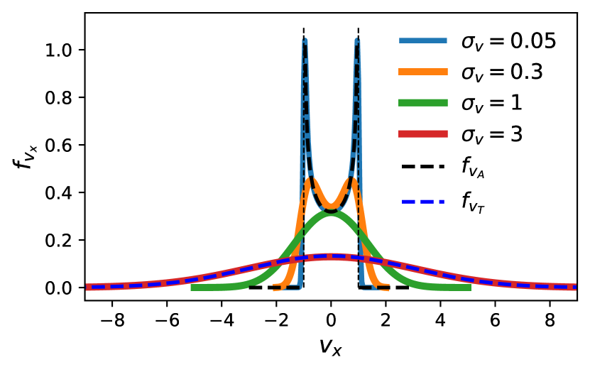
Figure 4: Velocity distribution along x-axis. The solid lines are numerical integrals of Eq. (9) with different $\sigma_{v}=v_{th}/v_{0}$ (here we set $v_{0}=1$ without loss of generality). Dashed lines are the PDFs of $f_{v_{A}}$ and $f_{v_{T}}$ indicated by black and blue, respectively.

From the discussions above, we can deduce that the single-peak/double-peak distributions are determined by the relative strength of effective thermal velocity to the active velocity, $\sigma_{v}$ in Eq. (10). This finding is consistent with the numerical integration of Eq. (9) with varying values of $\sigma_{v}$, see Fig. 4.

VI.2 Experimental results

Let’s first check the angular distributions. We find that the angular distributions for both heavy and light particles are indeed uniform, see Fig. 5 (b). The corresponding PDFs of $\cos\theta$ also fit the theoretical prediction, see Fig. 5 (a).

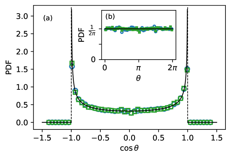
Figure 5: PDFs of of angles. Dots are experimental data of the PDF of $\cos\theta$ in (a) and the PDF of $\theta$ in (b). The solids lines are the theoretical predictions: for the PDF of $\cos\theta$, $f_{\cos\theta}(x)=\frac{1}{\pi\sqrt{1-x^{2}}},for\,x\in[-1,1];=0,\,else.$ For the PDF of $\theta$, $f_{\theta}(x)=\frac{1}{2\pi}$,uniformly distributed.

Then let’s test the velocity distributions. As shown in Fig. 6, the velocity distributions of the heavy particle exhibit single-peak, while the distributions of the light particle exhibit double-peak. Both of them can be well fitted by the minimal model, Eq. (9). The parameters of $v_{0}$ and $v_{th}$ are directly extracted from Table 1 without any fitting.

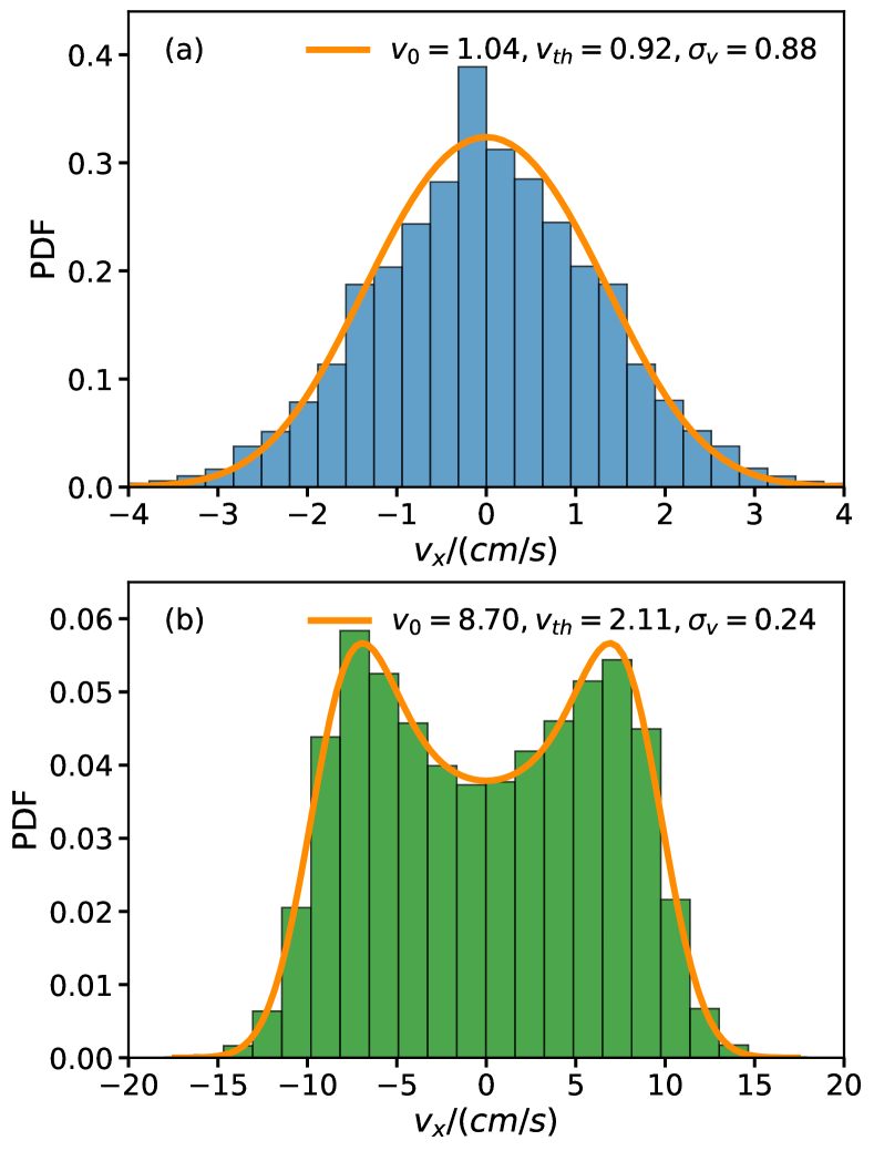
Figure 6: Experimental data of velocity distribution along x-axis. The PDF of the velocity of heavy particle exhibits single peak, as shown in histogram in (a). The PDF of the velocity of light particle exhibits double peak, as shown in histogram in (b). The orange solid lines are the theoretical predictions by Eq. (9), fitting the experimental PDFs, respectively. $v_{0}$ and $v_{th}=\sqrt{2D_{T}/h}$ are extracted from Table 1. $\sigma_{v}=v_{0}/v_{th}$ indicates the relative strenght of the active velocity over the translational noise velocity.

VII DISPLACEMENT DISTRIBUTIONS

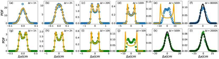
Figure 7: PDFs of the displacements for heavy (upper) and light (lower) particles. Dots are experiment data. Solid orange lines are the results from Eq. (14) with input values of time interval $\Delta t$ and $v_{0}$,$D_{T}$ in Tabel 1. Solid black lines are the results of the PDFs of long time diffusion $e^{-\Delta x^{2}/(4D_{eff}\Delta t)}/\sqrt{4\pi D_{eff}\Delta t}$ with the diffusivity in Eq. (5).

The minimal model can be directly extended to the displacement distributions in short time regimes, since the short-time displacement is

$$dx=v_{x}dt=v_{0}\cos\theta dt+\sqrt{2D_{T}}\xi_{x}dt.$$ (13)

The PDF of the displacements should be

$$f_{dx}(\Delta x)=\frac{1}{v_{0}dt}\int^{1}_{-1}\frac{1}{\pi\sqrt{1-u^{2}}}\frac{1}{\sqrt{2\pi}\sigma_{dx}}e^{-\frac{(\frac{\Delta x}{v_{0}dt}-u)^{2}}{2\sigma_{dx}^{2}}}du,$$ (14)

where the ratio of the effective thermal displacement to the active displacement is

$$\sigma_{dx}=\frac{\sqrt{2D_{T}dt}}{v_{0}dt}=\frac{\sqrt{2D_{T}/dt}}{v_{0}}.$$ (15)

Interestingly, Eq. (15) indicates that the PDF of the displacements could exhibit a crossover from the single-peak to the double-peak as the time interval increases. This could occur because the strength of the diffusion motion due to translational noise increases as $\propto\sqrt{dt}$, while the strength of the active motion increases as $\propto dt$. Consequently, the increase in time intervals effectively weakens the translational noise. Indeed, the crossover is observed in our experiments. The PDF of the displacements for the heavy particle clearly show the crossover from the single-peak to the double-peak until the time interval $\Delta t=100h$ , see Fig. 7 (a)-(d). The dots are experimental results, matching well with the numerical integration results from Eq. (14), as indicated in solid orange lines. For the long time intervals, Eq. (14) does not match the experimental data, because the displacement formula Eq. (13) is valid only for the short time intervals. For the long time intervals, the PDF of the displacements should become purely diffusive, which is also confirmed in our experiments. The PDF of the displacements in Fig. 7 (f) and (I) are fitted by the Gaussian distribution $\mathcal{N}(0,2D_{eff}\Delta t)$, as indicated by the solid black lines, where $D_{eff}$ is the long time diffusivity in Eq. (5).

VIII conclusions and discussion

We design 3D-printed motor driven active granular particles and find the particle dynamics can be characterized by the model of overdamped chiral ABPs, for both the rotational and translational MSDs. Then, we construct a minimal model that reproduces the double-peak velocity and displacement distributions. Our experiments validate the model.

A few remarks should be addressed. First of all, the minimal model is simple but quite useful. It not only reproduces the non-Gaussian diffusion phenomena, but also provides a clear mechanism: the interplay between the translational noise and active velocity leads to the observed crossover of single/double-peak distributions.

Second, to the best of our knowledge, the key angular statistical features of chirality, including the quadratic term $\Omega^{2}t^{2}$ in the long time angular MSDs, see Fig. 2 (e) and (f), and the oscillation term $\cos\Omega t$ in the ACFs of the directions, see Fig. 2 (g) and (h), have not been reported in experiments.

Third, the translational noise, often overlooked, is important as observed in our experiments. It not only causes a deviation from the expected $v_{0}^{2}t^{2}$ scaling in the MSD of the heavy particle in short time regimes, see Fig. 3, but also plays a critical role in the formation of the non-Gaussian distributions.

To summarize, our experiment using self-desiged, 3D-printed, motor-driven particles verifies the model of overdamped chiral ABPs. Our minimal model accurately describes the experimental results, and offers a clear physical picture of active induced non-Gaussian diffusion. Using our particles, future studies could explore how particle interactions and inertia modify this picture.