Alexandrov-Fenchel inequalities
for capillary hypersurfaces in hyperbolic space

Abstract.

In this article, we first introduce the quermassintegrals for compact hypersurfaces with capillary boundaries in hyperbolic space from a variational viewpoint, and then we solve an isoperimetric type problem in hyperbolic space. By constructing a new locally constrained inverse curvature flow, we obtain the Alexandrov-Fenchel inequalities for convex capillary hypersurfaces in hyperbolic space. This generalizes a theorem of Brendle-Guan-Li [11] for convex closed hypersurfaces in hyperbolic space.

Dedicated to Professor Guofang Wang on the occasion of his 60th birthday

1. Introduction

Let $\Omega$ be a convex body in hyperbolic space $\mathbb{H}^{n+1}$ with boundary $\partial\Omega$. The $k$-th quermassintegral of $\Omega$, denoted as $\mathcal{W}_{k}(\Omega)$, is defined as the volume of the set of totally geodesic $k$-dimensional subspaces that intersect $\Omega$ (see e.g. [42, Part IV] or [46]). In particular,

$$\mathcal{W}_{0}(\Omega)=|\Omega|,\leavevmode\nobreak\ \leavevmode\nobreak\ \leavevmode\nobreak\ \leavevmode\nobreak\ \mathcal{W}_{1}(\Omega)=\frac{1}{n+1}|\partial\Omega|.$$ (1.1)

If further assume that $\partial\Omega$ is smooth (say at least $C^{2}$), then the quermassintegrals $\mathcal{W}_{k}(\Omega)$ and the curvature integrals are related (see e.g. [46, Proposition 7]) by

$$\begin{aligned} \mathcal{W}_{k+1}(\Omega)=\frac{1}{n+1}\int_{\partial\Omega}H_{k}dA-\frac{k}{n+2-k}\mathcal{W}_{k-1}(\Omega),\leavevmode\nobreak\ 1\leq k\leq n-1.\end{aligned}$$ (1.2)

Here $H_{k}$ is the normalized $k$-th mean curvature of $\partial\Omega\subset\mathbb{H}^{n+1}$, see Section 2.1 for precise definition. The above quermassintegrals possess a nice variational structure (see e.g. [50, Proposition 3.1] or [7, Section 4]):

$$\frac{d}{dt}\mathcal{W}_{k}(\Omega_{t})=\frac{n+1-k}{n+1}\int_{\partial\Omega_{t}}fH_{k}dA_{t},\quad 0\leq k\leq n+1,$$ (1.3)

for any normal variation along $\partial\Omega_{t}$ with the speed function $f$. Furthermore, the Alexandrov-Fenchel inequalities involving the quermassintegrals $\mathcal{W}_{k}(\Omega)$ in hyperbolic space have attracted wide attention in recent decades, it states

$$\mathcal{W}_{k}(\Omega)\geq f_{k}\circ f^{-1}_{l}\left(\mathcal{W}_{l}(\Omega)\right),\leavevmode\nobreak\ 0\leq l<k\leq n,$$ (1.4)

where $f_{k}:[0,\infty)\rightarrow\mathbb{R}_{+}$ is the monotone function defined by $f_{k}(\rho):=\mathcal{W}_{k}(B_{\rho})$, with $B_{\rho}$ being the geodesic ball of radius $\rho$ in $\mathbb{H}^{n+1}$, and $f_{l}^{-1}$ being the inverse function of $f_{l}$. Moreover, the equality holds in (1.4) if and only if $\partial\Omega$ is a geodesic sphere. In [50], Wang-Xia studied a globally constrained quermassintegral preserving flow, given by one parameter family of embedded hypersurface $x(\cdot,t):M^{n}\times[0,T)\to\mathbb{H}^{n+1}$ satisfying

$$\partial_{t}x=\left(\frac{\int_{\partial\Omega_{t}}H_{k}^{\frac{1}{k-l}}H_{l}^{1-\frac{1}{k-l}}dA_{t}}{\int_{\partial\Omega_{t}}H_{l}dA_{t}}-\left(\frac{H_{k}}{H_{l}}\right)^{\frac{1}{k-l}}\right)\nu,\quad 0\leq l<k\leq n.$$ (1.5)

where $\nu=\nu(\cdot,t)$ is the unit outward normal of $x(\cdot,t)$. The flow (1.5) preserves $\mathcal{W}_{l}(\Omega_{t})$ while decreases $\mathcal{W}_{k}(\Omega_{t})$, then they established the Alexandrov-Fenchel inequalities (1.4) for $h$-convex domain $\Omega$ in $\mathbb{H}^{n+1}$ (cf. [50, Theorem 1.1]). Here a domain $\Omega\subset\mathbb{H}^{n+1}$ is referred to as $h$-convex if all the principal curvatures of its boundary $\partial\Omega$ are greater or equal to $1$. In other words, the minimum value of $\mathcal{W}_{k}(\Omega)$ among all the $h$-convex closed hypersurfaces $\partial\Omega$ in $\mathbb{H}^{n+1}$ with a fixed value $\mathcal{W}_{l}(\Omega)$ is achieved by the geodesic sphere. This solves a natural isoperimetric type problem for closed hypersurfaces in $\mathbb{H}^{n+1}$. In particular, when $k=1$ and $l=0$, (1.4) reduces to the classical isoperimetric inequality in $\mathbb{H}^{n+1}$ relating the area and volume, which was established by Schmidt in [45].

On the other hand, the hyperbolic space can be viewed as a warped product space $\mathbb{H}^{n+1}=[0,\infty)\times\mathbb{S}^{n}$, equipped with the metric

$$\bar{g}=d\rho^{2}+\phi^{2}(\rho)\sigma,$$

where $\phi(\rho)=\sinh\rho$ and $\sigma$ is the standard spherical metric on $\SS^{n}$. Based on the Minkowski formula (see e.g. Guan-Li [23, Proposition 2.5]) for the closed hypersurface $M:=\partial\Omega\subset\mathbb{H}^{n+1}$

$$\int_{M}(\phi^{\prime}H_{k-1}-vH_{k})dA=0,\leavevmode\nobreak\ \leavevmode\nobreak\ \leavevmode\nobreak\ 1\leq k\leq n,$$ (1.6)

where $\phi^{\prime}=\cosh\rho$ and $v$ is the support function of $M$ as

$$v=\bar{g}(\phi(\rho)\partial_{\rho},\nu).$$

In [11], Brendle-Guan-Li designed a locally constrained inverse curvature flow as

$$\partial_{t}x=\left(\frac{\phi^{\prime}}{F}-v\right)\nu,$$ (1.7)

where $F=\frac{H_{k}}{H_{k-1}}$. Along the flow (1.7), when the evolving hypersurfaces are $k$-convex, then the $k$-th quermassintegral $\mathcal{W}_{k}(\Omega_{t})$ is preserved and the $(k+1)$-th quermassintegral $\mathcal{W}_{k+1}(\Omega_{t})$ is non-increasing with respect to the time $t\geq 0$. Here a smooth hypersurface $M\subset\mathbb{H}^{n+1}$ is $k$-convex for some $1\leq k\leq n$ means that its principal curvatures $\kappa:=(\kappa_{1},\cdots,\kappa_{n})\in\Gamma_{k}$, see (2.1). A smooth hypersurface $M\subset\mathbb{H}^{n+1}$ is called star-shaped if its support function $v$ is positive everywhere on $M$. In [11, Theorem 1.3], Brendle-Guan-Li established the long-time existence and convergence of flow (1.7) under two cases: either the initial closed hypersurface $M_{0}$ is strictly convex and $k=n$ or $M_{0}$ is star-shaped, $k$-convex and satisfying a gradient bound condition. As a consequence, the inequalities (1.4) holds for $k=n$ and $0\leq l\leq n-1$ provided that $\partial\Omega$ is convex. Recently, Hu-Li-Wei [26, Theorem 1.1] obtained the long-time existence and convergence of flow (1.7) when $M_{0}$ is a $h$-convexity for all $1\leq k\leq n$, which also provided an alternative proof of the inequalities (1.4) for $h$-convex domain $\Omega\subset\mathbb{H}^{n+1}$. It is a challenging problem to prove that inequalities (1.4) hold for a domain under the weak geometric assumption, say for instance assuming $\partial\Omega$ is $(k-1)$-convex and star-shaped, which is an analogous known condition to be true for the Alexandrov-Fenchel inequality in Euclidean space (cf. Guan-Li [22, Theorem 2]). Nevertheless, there have been some efforts and partial results in this direction. Li-Wei-Xiong [32, Theorem 1] demonstrated that when $k=3$ and $l=1$, (1.4) holds for $\partial\Omega$ being $2$-convex and star-shaped. Andrews-Chen-Wei [3, Corollary 1.5] established (1.4) with $k=1,\cdots,n$ and $l=0$ for a domain with boundary having positive intrinsic curvatures, which by Gauss equation is equivalent to the principal curvatures of $\partial\Omega$ satisfying $\kappa_{i}\kappa_{j}>1$ for $1\leq i\neq j\leq n$. This is again a weaker condition than $h$-convexity. Andrews-Hu-Li [4, Corollary 1.2] showed that (1.4) holds for a strictly convex domain with $k=n-1$ and $l=n-1-2m$ $(0<2m<n)$. For more related progress in hyperbolic space, one can refer to [6, 8, 9, 12, 15, 18, 20, 21, 23, 24, 25, 36, 44, 53] and references therein.

Meanwhile, there has been growing interest in investigating geometric variational problems for compact hypersurfaces with non-empty boundaries in recent decades, such as hypersurfaces with free or general capillary boundaries in Euclidean space. Especially the studies have focused on isoperimetric type problems (see [10, 13, 17, 34, 35] etc.) and Alexandrov-Fenchel type inequalities (see [28, 43, 54, 48] etc.) for these hypersurfaces in Euclidean space. In particular, Scheuer-Wang-Xia introduced the concept of quermassintegrals for compact hypersurfaces with free boundaries in the Euclidean unit ball $\bar{\mathbb{B}}^{n+1}$ from a variational perspective in [43]. Then they established the Alexandrov-Fenchel inequalities and Gauss-Bonnet-Chern theorem for these quantities, which can be viewed as higher-order generalizations of the relative isoperimetric inequality in $\bar{\mathbb{B}}^{n+1}$ (cf. [14, Theorem 18.1.3]). They achieved this new family of Alexandrov-Fenchel inequalities for convex hypersurfaces in $\bar{\mathbb{B}}^{n+1}$ with free boundaries by constructing a locally constrained inverse curvature flow, which is motivated by the Minkowski formula for free boundary hypersurface in [51, Proposition 5.1]. Subsequently, Weng-Xia [54] defined the analogous concept of the quermassintegrals for capillary hypersurfaces in $\bar{\mathbb{B}}^{n+1}$, then they obtained the Alexandrov-Fenchel type inequalities and Gauss-Bonnet-Chern theorem in the capillary setting of $\bar{\mathbb{B}}^{n+1}$. Very recently, Wang-Weng-Xia [48] introduced the quermassintegrals for compact hypersurfaces with capillary boundary in the Euclidean half-space $\overline{\mathbb{R}^{n+1}_{+}}$, and further derived the Alexandrov-Fenchel inequalities for those capillary hypersurfaces. It turns out those new quantities in $\overline{\mathbb{R}^{n+1}_{+}}$ can also be interpreted from the viewpoint of convex geometry, as shown in [38, Section 2.2]. For more related results, we recommend the readers refer to [27, 28, 30, 31, 35, 37, 38, 39, 41, 48, 49, 52] and references therein.

Based on the aforementioned results, a natural question arises regarding the corresponding geometric variational problem, specifically the isoperimetric type problems, for compact hypersurface with non-empty boundaries in hyperbolic space. This paper’s primary objective is to first introduce the quermassintegrals for capillary hypersurfaces supported on totally geodesic hyperplanes in hyperbolic space $\mathbb{H}^{n+1}$. Subsequently, we establish the Alexandrov-Fenchel inequalities (a higher-order isoperimetric type inequality) for these quantities in $\mathbb{H}^{n+1}$. To describe our results, we introduce some notations and definitions. We employ the Poincaré ball model to represent the hyperbolic space $\mathbb{H}^{n+1}$, denoted by $\left(\mathbb{B}^{n+1},\bar{g}\right)$ with

$$\mathbb{B}^{n+1}=\{x\in\mathbb{R}^{n+1}:|x|<1\},\quad\bar{g}=e^{2u}\delta,\leavevmode\nobreak\ \leavevmode\nobreak\ \leavevmode\nobreak\ \leavevmode\nobreak\ e^{2u}:=\frac{4}{(1-|x|^{2})^{2}},$$

where $\delta$ is the standard Euclidean metric. The supported totally geodesic hyperplane is given by

$$\mathcal{H}:=\{x\in\mathbb{B}^{n+1}:\delta(x,E_{n+1})=0\},$$

where $E_{n+1}=(0,\cdots,0,1)$ is the $(n+1)$-th coordinate basis in $\mathbb{B}^{n+1}$. We further denote

$$\mathcal{H}^{+}:=\{x\in\mathbb{B}^{n+1}:\delta(x,E_{n+1})\geq 0\}.$$

Let $\Sigma$ be an embedded hypersurface in ${\mathcal{H}^{+}}$ satisfying

$${\rm{int}}(\Sigma)\subset{\rm int}(\mathcal{H}^{+})\quad\text{and}\quad\partial\Sigma\subset\mathcal{H}.$$ (1.8)

We denote $\widehat{\Sigma}$ as the bounded domain enclosed by $\Sigma$ and the totally geodesic hyperplane $\mathcal{H}$ in $\mathcal{H}^{+}$ and $\widehat{\partial\Sigma}$ as the bounded domain enclosed by $\partial\Sigma$ inside $\mathcal{H}$, see Figure 1. Without loss of generality, throughout this paper, we assume that the origin point $O\in\text{int}(\widehat{\partial\Sigma})$.

Definition 1.1.

A compact hypersurface $\Sigma\subset{{\mathcal{H}}^{+}}$ is called a capillary hypersurface if it satisfies (1.8) and intersects with $\mathcal{H}$ at a constant contact angle $\theta\in(0,\pi)$ along $\partial\Sigma\cap\mathcal{H}$.

The simplest example of capillary hypersurface in $\mathbb{H}^{n+1}$ is a family of geodesic spherical caps lying entirely in ${\mathcal{H}^{+}}$ and intersecting with $\mathcal{H}$ at a constant contact angle $\theta\in(0,\frac{\pi}{2})$, which is given by

$$\mathcal{C}_{\theta,r_{0}}:=\left\{x\in{\mathcal{H}^{+}}:|x+r_{0}\cos\theta E_{n+1}|=r_{0}\right\},\leavevmode\nobreak\ \text{for}\leavevmode\nobreak\ 0<r_{0}<\frac{1}{\sin\theta}.$$ (1.9)

It is clear that the constraint $0<r_{0}<\frac{1}{\sin\theta}$ is a necessary and sufficient condition for $\mathcal{C}_{\theta,r_{0}}$ lying in the unit ball.

Inspired by the recent progress about the capillary hypersurface in Euclidean space as [43, 54] and [48], we first introduce a family of new geometric quantities (Quermassintegrals) $\mathcal{A}_{k,\theta}(\widehat{\Sigma})$ for capillary hypersurface $\Sigma$ in $\mathbb{H}^{n+1}$ in this paper. Before that, we fix some notations for the $(n+1)$-dimensional convex body $\widehat{\Sigma}\subset\mathbb{H}^{n+1}$. Parallel to (1.1) and (1.2), we denote

$$\begin{aligned} &\mathcal{W}_{0}(\widehat{\Sigma}):=|\widehat{\Sigma}|,\quad\leavevmode\nobreak\ \leavevmode\nobreak\ \mathcal{W}_{1}(\widehat{\Sigma}):=\frac{1}{n+1}|\Sigma|,\\ &\mathcal{W}_{k+1}(\widehat{\Sigma})=\frac{1}{n+1}\int_{\Sigma}H_{k}dA-\frac{k}{n+2-k}\mathcal{W}_{k-1}(\widehat{\Sigma}),\leavevmode\nobreak\ 1\leq k\leq n-1,\end{aligned}$$

where $H_{k}$ is the normalized $k$-th mean curvature of $\Sigma\subset\mathcal{H}^{+}$. Similarly, we have the quermassintegrals for the $n$-dimensional convex body $\widehat{\partial\Sigma}\subset\mathcal{H}\subset\mathbb{H}^{n+1}$, which are defined by

$$\mathcal{W}_{0}^{\mathcal{H}}(\widehat{\partial\Sigma}):=|\widehat{\partial\Sigma}|,\quad\quad\mathcal{W}_{1}^{\mathcal{H}}(\widehat{\partial\Sigma}):=\frac{1}{n}|\partial\Sigma|,$$

$$\mathcal{W}_{k+1}^{\mathcal{H}}(\widehat{\partial\Sigma})=\frac{1}{n}\int_{\partial\Sigma}H_{k}^{\partial\Sigma}ds-\frac{k}{n+1-k}\mathcal{W}^{\mathcal{H}}_{k-1}(\widehat{\partial\Sigma}),\leavevmode\nobreak\ 1\leq k\leq n-2,$$

where $H_{k}^{\partial\Sigma}:=\frac{1}{\binom{n-1}{k}}\sigma^{\partial\Sigma}_{k}$ is the normalized $k$-th mean curvature of $\partial\Sigma\subset\mathcal{H}$.

Now we are ready to introduce the quermassintegrals $\mathcal{A}_{k,\theta}(\widehat{\Sigma})$ for capillary hypersurface $\Sigma$ in $\mathbb{H}^{n+1}$ as

$$\mathcal{A}_{0,\theta}(\widehat{\Sigma}):=\mathcal{W}_{0}(\widehat{\Sigma}),\leavevmode\nobreak\ \leavevmode\nobreak\ \mathcal{A}_{1,\theta}(\widehat{\Sigma}):=\mathcal{W}_{1}(\widehat{\Sigma})-\frac{\cos\theta}{n+1}\mathcal{W}_{0}^{\mathcal{H}}(\widehat{\partial\Sigma}),$$

and for $1\leq k\leq n-1$,

$$\mathcal{A}_{k+1,\theta}(\widehat{\Sigma}):=\mathcal{W}_{k+1}(\widehat{\Sigma})+\frac{\cos\theta}{n+1}\sum\limits_{l=0}^{[\frac{k}{2}]}(-1)^{l-1}(\sin\theta)^{k-2l}\cdot\mathcal{W}_{k-2l}^{\mathcal{H}}(\widehat{\partial\Sigma})\prod_{s=0}^{l-1}\frac{k-2s}{n-k+2(s+1)},\leavevmode\nobreak\ \leavevmode\nobreak\ \leavevmode\nobreak\ \leavevmode\nobreak\ \leavevmode\nobreak\ \leavevmode\nobreak\ \leavevmode\nobreak\$$ (1.10)

where we have used the convention that $\prod\limits_{s=0}^{-1}\cdot=1$.

When $\theta=\frac{\pi}{2}$, it is easy to see that $\mathcal{A}_{k+1,\theta}(\widehat{\Sigma})=\mathcal{W}_{k+1}(\widehat{\Sigma})$ for all $-1\leq k\leq n$, which make us to expect that $\mathcal{A}_{k+1,\theta}(\widehat{\Sigma})$ would be the correct capillary counterpart of the quermassintegrals for the closed hypersurfaces in $\mathbb{H}^{n+1}$. Besides, the following first variational formula is the motivation for us to define $\mathcal{A}_{k,\theta}(\widehat{\Sigma})$ as the quermassintegrals for capillary hypersurface in $\mathbb{H}^{n+1}$.

Theorem 1.2.

Let $\Sigma_{t}\subset{{\mathcal{H}}^{+}}$ be a family of smooth capillary hypersurfaces, given by embeddings $x(\cdot,t):M\rightarrow{{\mathcal{H}}^{+}}$ and satisfying

$$(\partial_{t}x)^{\perp}=f\nu,$$

for some smooth function $f$. Then for $0\leq k\leq n$,

$$\frac{d}{dt}\mathcal{A}_{k,\theta}(\widehat{\Sigma_{t}})=\frac{n+1-k}{n+1}\int_{\Sigma_{t}}fH_{k}dA_{t}.$$

Furthermore, we establish the Alexandrov-Fenchel inequalities for the quermassintegrals $\mathcal{A}_{k,\theta}(\widehat{\Sigma})$, when $\Sigma$ is a convex capillary hypersurface in $\mathbb{H}^{n+1}$ and $\theta\in(0,\frac{\pi}{2}]$.

Theorem 1.3.

For $n\geq 2$, let $\Sigma\subset{{\mathcal{H}}^{+}}$ be a convex capillary hypersurface with contact angle $\theta\in(0,\frac{\pi}{2}]$. Assume that

there exists a geodesic spherical cap $$\mathcal{C}_{\theta,r_{0}} \Sigma\subset\widehat{\mathcal{C}_{\theta,r_{0}}}$$ such that . (1.11)

Then there holds

$$\mathcal{A}_{n,\theta}(\widehat{\Sigma})\geq(f_{n,\theta}\circ f_{k,\theta}^{-1})\left(\mathcal{A}_{k,\theta}(\widehat{\Sigma})\right),\quad\forall\leavevmode\nobreak\ 1\leavevmode\nobreak\ \leq k\leq n-1,$$ (1.12)

where $f_{k,\theta}:[0,\infty)\rightarrow\mathbb{R}_{+}$ is a strictly monotone function defined by

$$f_{k,\theta}(r):=\mathcal{A}_{k,\theta}(\widehat{\mathcal{C}_{\theta,r}}),$$

where $\mathcal{C}_{\theta,r}$ is the geodesic spherical cap given by (1.9). Moreover, equality holds if and only if $\Sigma$ is a geodesic spherical cap.

In other words, the maximum value of $\mathcal{A}_{k,\theta}(\widehat{\Sigma})$ among all the convex capillary hypersurfaces $\Sigma\subset\mathbb{H}^{n+1}$ with a fixed value $\mathcal{A}_{n,\theta}(\widehat{\Sigma})$ is achieved by the geodesic spherical caps. This solves an isoperimetric type problem for compact hypersurfaces with non-empty boundaries in $\mathbb{H}^{n+1}$. In particular, when $\theta=\frac{\pi}{2}$, by a simple reflection argument of $\Sigma$ along $\mathcal{H}$, (1.12) recovers the Alexandrov-Fenchel inequalities between $\mathcal{W}_{k}$ and $\mathcal{W}_{n}$ for convex closed hypersurface in $\mathbb{H}^{n+1}$, as shown in [11, Theorem 1.4]. Furthermore, when $n=2$, from (1.12), we obtain a Minkowski-type inequality for convex capillary surface $\Sigma$ in $\mathbb{H}^{3}$.

Corollary 1.4.

Let $\Sigma\subset\mathcal{H}^{+}$ be a convex capillary surface with contact angle $\theta\in(0,\frac{\pi}{2}]$, and $\Sigma$ satisfies (1.11). Then

$$\int_{\Sigma}HdA\geq 2|\widehat{\Sigma}|+6\leavevmode\nobreak\ (f_{2,\theta}\circ f_{1,\theta}^{-1})\left(\frac{1}{3}\left(|\Sigma|-\cos\theta|\widehat{\partial\Sigma}|\right)\right)+\sin\theta\cos\theta|\partial\Sigma|.$$ (1.13)

Moreover, equality holds if and only if $\Sigma$ is a geodesic spherical cap.

In order to prove Theorem 1.3, we construct a locally constrained inverse curvature flow as described in (3.1) and (3.4), inspired by the ideas of Brendle-Guan-Li in [11] and the Minkowski formula (2.6) by Chen-Pyo [16] for capillary hypersurfaces in $\mathbb{H}^{n+1}$. We demonstrate that if the initial capillary hypersurface is strictly convex, the flow exists for all time $t\in[0,\infty)$, preserves the convexity, and smoothly converges to a geodesic spherical cap, as stated in Theorem 3.2. A key ingredient to show Theorem 3.2 is obtaining the uniform curvature estimates, particularly the two-sided uniform bound for $F$. For this, we introduce the capillary support function $\widetilde{v}$ as (3.32) for capillary hypersurfaces $\Sigma$ in $\mathbb{H}^{n+1}$, i.e.

$$\widetilde{v}=\frac{\bar{g}(x,\nu)}{V_{0}-\cos\theta\bar{g}(Y_{n+1},\nu)},$$

which satisfies a nice homogeneous Neumann boundary value condition along $\partial\Sigma$, as shown in (3.34). Moreover, along the flow (3.1), we show that quermassintegral $\mathcal{A}_{n,\theta}(\widehat{\Sigma_{t}})$ is preserved, while $\mathcal{A}_{k,\theta}(\widehat{\Sigma_{t}})$ $(1\leq k\leq n-1)$ is non-decreasing for $t\geq 0$. This allows us to complete the proof of Theorem 1.3, by combining Theorem 3.2. We note that the condition $\theta\leq\frac{\pi}{2}$ is a technical assumption necessary to ensure the boundary curvature estimate of the flow, as seen in (3.40), which is the only place we used this condition. This angle restriction is similarly required and crucially utilized in [27, 28, 48, 54] etc. Finally, we point out that the assumption (1.11) ensures the existence of a geodesic spherical cap that bounds the capillary hypersurface from the exterior, which may not generally be true for convex capillary hypersurfaces $\Sigma\subset\mathcal{H}^{+}$ with boundaries $\partial\Sigma$ close to $\mathcal{H}\cap\partial\mathbb{B}^{n+1}$. Given this natural assumption, it is evident that it will be preserved for all evolving convex capillary hypersurfaces by the avoidance principle along the flow (3.1) starting from such initial datum, as stated in Proposition 3.10.

The rest of the article is structured as follows. In Section 2, we recall some basic properties of elementary symmetric polynomial functions. Subsequently, we introduce relevant notations and basic properties regarding capillary hypersurfaces supported on the geodesic hyperplane $\mathcal{H}$ in $\mathbb{H}^{n+1}$. Then we present the first variational formula of quermassintegrals $\mathcal{A}_{k,\theta}$ and complete the proof of Theorem 1.2. In Section 3, we introduce the locally constrained inverse curvature flow (3.1) and analyze the long-time existence and convergence of such flow. The last section is devoted to proving the Alexandrov-Fenchel inequalities for convex capillary hypersurfaces in $\mathbb{H}^{n+1}$, i.e., Theorem 1.3.

2. Quermassintegrals and first variational formula

2.1. Elementary symmetric polynomial functions

In this subsection, we recall some well-known properties of the $k$-th elementary symmetric functions. Let $A=\{A_{ij}\}$ be an $n\times n$ symmetric matrix, and $k\in\{1,2,\cdots,n\}$, define

$$\sigma_{k}(A):=\sigma_{k}(\lambda(A))=\sum\limits_{1\leq i_{1}<i_{2}\cdots<i_{k}\leq n}\lambda_{i_{1}}\lambda_{i_{2}}\cdots\lambda_{i_{k}},$$

where $\lambda:=\lambda(A)=(\lambda_{1},\cdots,\lambda_{n})$ is the eigenvalues of $A$. We use the convention that $\sigma_{0}=1$ and $\sigma_{k}=0$ for $k>n$. Let $H_{k}(A):=H_{k}(\lambda(A))$ be the normalization of $\sigma_{k}(\lambda)$ given by

$$H_{k}(\lambda)=\frac{1}{\binom{n}{k}}\sigma_{k}(\lambda).$$

Denote $\sigma_{k}(\lambda\left|i\right.)$ the symmetric polynomial function of $\sigma_{k}(\lambda)$ with $\lambda_{i}=0$ and $\sigma_{k}(\lambda\left|ij\right.)$ the symmetric polynomial function of $\sigma_{k}(\lambda)$ with $\lambda_{i}=\lambda_{j}=0$. Recall that Gårding’s cone is defined as

$$\Gamma_{k}=\{\lambda\in\mathbb{R}^{n}:\sigma_{i}(\lambda)>0,\leavevmode\nobreak\ \leavevmode\nobreak\ \forall 1\leq i\leq k\}.$$ (2.1)

Lemma 2.1.

Let $\lambda=(\lambda_{1},\cdots,\lambda_{n})\in\mathbb{R}^{n}$ and $k=1,\ldots,n$. Then

1. $\sigma_{k}(\lambda)=\sigma_{k}(\lambda|i)+\lambda_{i}\sigma_{k-1}(\lambda|i),\quad\forall 1\leq i\leq n.$

2. $\sum\limits_{i=1}^{n}{\sigma_{k}(\lambda|i)}=(n-k)\sigma_{k}(\lambda).$

3. $\sum\limits_{i=1}^{n}{\lambda_{i}\sigma_{k-1}(\lambda|i)}=k\sigma_{k}(\lambda)$.

4. $\sum\limits_{i=1}^{n}{\lambda_{i}^{2}\sigma_{k-1}(\lambda|i)}=\sigma_{1}(\lambda)\sigma_{k}(\lambda)-(k+1)\sigma_{k+1}(\lambda)$.

We denote $\sigma_{k}(A\left|i\right.)$ the $\sigma_{k}$ symmetric polynomial function of the matrix obtained from $A$ by deleting the $i$-row and $i$-column and $\sigma_{k}(A\left|ij\right.)$ the $\sigma_{k}$ symmetric polynomial function of the matrix from $A$ by deleting the $i,j$-rows and $i,j$-columns.

Lemma 2.2.

Suppose that $A=\{A_{ij}\}$ is diagonal, and $k$ is a positive integer. Then

$$\sigma_{k-1}^{ij}(A)=\begin{cases}\sigma_{k-1}(A\left|i\right.),&\text{if }i=j,\\ 0,&\text{if }i\neq j,\end{cases}$$

where $\sigma_{k-1}^{ij}(A):=\frac{{\partial\sigma_{k}(A)}}{{\partial A_{ij}}}$.

Lemma 2.3.

The following properties hold.

1. For $\lambda\in\Gamma_{k}$ and $k>l\geq 0$, $r>s\geq 0$, $k\geq r$, $l\geq s$, there holds the generalized Newton-Maclaurin inequality

   $$\left(\frac{H_{k}(\lambda)}{H_{l}(\lambda)}\right)^{\frac{1}{k-l}}\leq\left(\frac{H_{r}(\lambda)}{H_{s}(\lambda)}\right)^{\frac{1}{r-s}},$$

   with equality holds if and only if $\lambda_{1}=\lambda_{2}=\cdots=\lambda_{n}>0$.

2. For $0\leq l<k\leq n$, then $\left(\frac{H_{k}(\lambda)}{H_{l}(\lambda)}\right)^{\frac{1}{k-l}}$ is a concave function with respect to $\lambda\in\Gamma_{k}$.

3. For $0\leq l<k\leq n$, and $F(\lambda)=\left(\frac{H_{k}(\lambda)}{H_{l}(\lambda)}\right)^{\frac{1}{k-l}}$. Assume $\lambda=(\lambda_{1},\cdots,\lambda_{n})$ satisfies $\lambda_{1}\geq\lambda_{2}\geq\cdots\geq\lambda_{n}$. Then

   $$\frac{\partial F(\lambda)}{\partial\lambda_{1}}\leq\frac{\partial F(\lambda)}{\partial\lambda_{2}}\leq\cdots\leq\frac{\partial F(\lambda)}{\partial\lambda_{n}}.$$

For proof of the above Lemmas, see e.g. [33, Chapter XV, Section 4] and [47, Lemma 2.10, Theorem 2.11, Lemma 1.5].

2.2. Notation and conventions

We use $D$ to denote the Levi-Civita connection of $\mathcal{H}^{+}$ w.r.t the metric $\bar{g}$, and $\nabla$ represents the Levi-Civita connection on $\Sigma$ w.r.t the induced metric $g$ from the immersion $x$. The operators ${\rm div},\Delta$, and $\nabla^{2}$ are the divergence, Laplacian, and Hessian operators on $\Sigma$ respectively. The second fundamental form $h$ of $x$ is defined by

$$D_{X}Y=\nabla_{X}Y-h(X,Y)\nu.$$

The Weingarten operator is defined via $\bar{g}(\mathcal{W}(X),Y)=h(X,Y),$ and the Weingarten equation is

$$D_{X}\nu=\mathcal{W}(X).$$

We shall use the convention of Einstein summation. For convenience the components of the Weingarten map $\mathcal{W}$ are denoted by $(h^{i}_{j})=(g^{ik}h_{kj})$, and $|h|^{2}$ be the norm square of the second fundamental form, that is $|h|^{2}=g^{ik}h_{kl}h_{ij}g^{jl}$, where $(g^{ij})$ is the inverse of $(g_{ij})$. We use the metric tensor $(g_{ij})$ and its inverse $(g^{ij})$ to lower down and raise up the indices of tensor fields on $\Sigma$.

2.3. Convex capillary hypersurfaces in $\mathbb{H}^{n+1}$

Let $\Sigma\subset{{\mathcal{H}}^{+}}$ be a smooth capillary hypersurface, given by the embedding $x:M\to{{\mathcal{H}}^{+}}$, if without cause confusion, we do not distinguish $\Sigma$ and the embedding $x$. Let $\mu$ be the unit outward co-normal of $\partial\Sigma$ in $\Sigma$ and $\overline{\nu}$ be the unit normal to $\partial\Sigma$ in $\mathcal{H}$ such that $\{\nu,\mu\}$ and $\{\overline{\nu},\overline{N}\}$ have the same orientation in normal bundle of $\partial\Sigma\subset{{\mathcal{H}}^{+}}$, where $\overline{N}$ is the unit outward normal of $\mathcal{H}\subset{\mathcal{H}}^{+}$. See Figure 1. From Definition 1.1,

$$\bar{g}(\nu,\overline{N})=\cos(\pi-\theta).$$ (2.2)

It follows

$$\begin{array}[]{rcl}\overline{N}&=&\sin\theta\mu-\cos\theta\nu,\\ \overline{\nu}&=&\cos\theta\mu+\sin\theta\nu.\end{array}$$ (2.5)

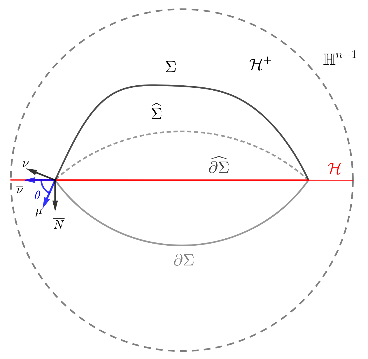
Figure 1. Figure 1. A capillary hypersurface $\Sigma\subset\mathbb{H}^{n+1}$ supported on $\mathcal{H}$.

The second fundamental form of $\partial\Sigma$ in $\mathcal{H}$ is given by

$$\widehat{h}(X,Y):=\bar{g}(\nabla^{\mathbb{H}^{n}}_{X}\overline{\nu},Y)=\bar{g}(D_{X}\overline{\nu},Y),\quad X,Y\in T(\partial\Sigma).$$

The second fundamental form of $\partial\Sigma$ in $\Sigma$ is given by

$$\widetilde{h}(X,Y):=\bar{g}(\nabla_{X}\mu,Y)=\bar{g}(D_{X}\mu,Y),\quad X,Y\in T(\partial\Sigma).$$

It turns out that $\widehat{h},\widetilde{h}$ and $h$ have a nice relationship. The similar properties were previously established by Wang-Weng-Xia in [48, Proposition 2.2] for the capillary hypersurface in $\overline{\mathbb{R}^{n+1}_{+}}$.

Proposition 2.4.

Let $\Sigma\subset{\mathcal{H}^{+}}$ be a smooth capillary hypersurface and $\{e_{\alpha}\}_{\alpha=2}^{n}$ be an orthonormal frame of $\partial\Sigma$. Then along $\partial\Sigma$,

• $\mu$ is a principal direction of $\Sigma$. That is, $h_{\mu\alpha}:=h(\mu,e_{\alpha})=0$.

• $h_{\alpha\beta}=\sin\theta\widehat{h}_{\alpha\beta}.$

• $\widetilde{h}_{\alpha\beta}=\cos\theta\widehat{h}_{\alpha\beta}=\cot\theta h_{\alpha\beta}.$

• $\nabla_{\mu}h_{\alpha\beta}=\widetilde{h}_{\beta\gamma}(h_{\mu\mu}\delta_{\alpha\gamma}-h_{\alpha\gamma})$.

Proof.

The first and fourth assertions are well-known, see e.g. [1, Lemma 2.2] and [48, Proposition 2.4 (4)] resp. While (2) and (3) follow from (2.5) and the simple fact that $\mathcal{H}$ is totally geodesic hyperplane in $\mathbb{H}^{n+1}$. In fact,

$$\widehat{h}_{\alpha\beta}=\bar{g}(D_{e_{\alpha}}\overline{\nu},e_{\beta})=\bar{g}(D_{e_{\alpha}}(\cot\theta\overline{N}+\csc\theta\nu),e_{\beta})=\csc\theta h_{\alpha\beta},$$

and

$$\widetilde{h}_{\alpha\beta}=\bar{g}(D_{e_{\alpha}}\mu,e_{\beta})=\bar{g}(D_{e_{\alpha}}(\csc\theta\overline{N}+\cot\theta\nu),e_{\beta})=\cot\theta h_{\alpha\beta}.$$

∎

Corollary 2.5.

Let $\Sigma\subset{\mathcal{H}^{+}}$ be a smooth capillary hypersurface with a constant angle $\theta\in(0,\frac{\pi}{2})$. If $\Sigma$ is convex (resp. strictly convex), in the sense that $h$ is non-negative definite (resp. positive definite), then $\partial\Sigma$ is convex (resp. strictly convex) in both $\Sigma$ and $\mathcal{H}$.

Chen-Pyo had established the following Minkowski type formula [16, Proposition 3], which can be viewed as the capillary analogous result of (1.6) in $\mathbb{H}^{n+1}$. This formula will be important in constructing the locally constrained curvature flow later.

Proposition 2.6 ([16]).

Let $x:M\rightarrow{{\mathcal{H}}^{+}}$ be a smooth immersion of $\Sigma:=x(M)$ into ${{\mathcal{H}}^{+}}$, and its boundary intersects with $\mathcal{H}$ at a constant angle $\theta\in(0,\pi)$. Then for any $1\leq k\leq n$, there holds

$$\int_{\Sigma}\left[H_{k-1}(V_{0}-\cos\theta\bar{g}(Y_{n+1},\nu))-H_{k}\bar{g}(x,\nu)\right]dA=0,$$ (2.6)

where $V_{0}=\frac{1+|x|^{2}}{1-|x|^{2}}$, $Y_{n+1}$ is a Killing vector field in $\mathbb{H}^{n+1}$, given by

$$Y_{n+1}:=\frac{1}{2}(1+|x|^{2})E_{n+1}-\delta(x,E_{n+1})x,$$ (2.7)

and $dA$ is the area element of $\Sigma$ w.r.t. the induced metric.

Next, we demonstrate that the spherical cap $\mathcal{C}_{\theta,r_{0}}$ is an umbilical capillary hypersurface in $\mathcal{H}^{+}$ such that the integrand in (2.6) is identically zero. In particular, this implies that the geodesic spherical caps are the static solutions to our flow (3.4) in the next Section.

Proposition 2.7.

For any $r_{0}>0$, the geodesic spherical cap $\mathcal{C}_{\theta,r_{0}}$ defined in (1.9) satisfies

$$V_{0}-\cos\theta\bar{g}(Y_{n+1},\nu)-\frac{1+r^{2}_{0}\sin^{2}\theta}{2r_{0}}\bar{g}(x,\nu)=0,$$ (2.8)

and its principal curvatures equal $\frac{H_{k}}{H_{k-1}}=\frac{1+r^{2}_{0}\sin^{2}\theta}{2r_{0}}$ for all $1\leq k\leq n$.

Proof.

For any $x\in\mathcal{C}_{\theta,r_{0}}$, we know

$$\cos\theta\bar{g}(Y_{n+1},\nu) = \frac{4\cos\theta}{(1-|x|^{2})^{2}}\left(\frac{1}{2}(1+|x|^{2})\delta(E_{n+1},\nu)-\delta(x,E_{n+1})\delta(x,\nu)\right)$$ (2.9)

$$= \frac{r^{2}_{0}\cos^{2}\theta+r^{2}_{0}-|x|^{2}+r^{2}_{0}|x|^{2}\cos^{2}\theta+r^{2}_{0}|x|^{2}-r^{4}_{0}\sin^{4}\theta}{2(1-|x|^{2})r^{2}_{0}},$$

and

$$\bar{g}(x,\nu)=\frac{4}{(1-|x|^{2})^{2}}\delta(x,\nu)=\frac{|x|^{2}+r^{2}_{0}\sin^{2}\theta}{r_{0}(1-|x|^{2})}.$$ (2.10)

Combining (2.9), (2.10) and $V_{0}=\frac{1+|x|^{2}}{1-|x|^{2}}$, it follows (2.8). Using [52, formula (13)], the spherical cap $\mathcal{C}_{\theta,r_{0}}$ is umbilical in ${\mathcal{H}}^{+}$ and the principal curvatures are equal to $\frac{1+r^{2}_{0}\sin^{2}\theta}{2r_{0}}$, then the assertion is proved. ∎

2.4. Quermassintegrals and the first variational formula

We introduce the quermassintegrals $\mathcal{A}_{k,\theta}(\widehat{\Sigma})$ as (1.10) for compact hypersurface with capillary boundary supported on the geodesic hyperplane in $\mathbb{H}^{n+1}$. The definition of the quermassintegrals $\mathcal{A}_{k,\theta}(\widehat{\Sigma})$ in such a way is motivated by the first variational formula. For the reader’s convenience, we restate Theorem 1.2 in the following.

Theorem 2.8.

Let $\Sigma_{t}\subset{\mathcal{H}^{+}}$ be a family of smooth hypersurfaces with capillary boundary supported on $\mathcal{H}$, given by the embedding $x(\cdot,t):M\rightarrow{\mathcal{H}^{+}}$ and satisfies

$$(\partial_{t}x)^{\perp}=f\nu,$$ (2.11)

for some smooth function $f$. Then for $-1\leq k\leq n-1$,

$$\frac{d}{dt}\left(\mathcal{A}_{k+1,\theta}(\widehat{\Sigma_{t}})\right)=\frac{n-k}{n+1}\int_{\Sigma_{t}}fH_{k+1}dA_{t}.$$ (2.12)

Before proving Theorem 2.8, we rewrite the flow (2.11) in the following general form

$$\partial_{t}x=f\nu+\mathcal{T},$$ (2.13)

where $\mathcal{T}$ is the tangential vector along $T\Sigma_{t}$. If further imposing the capillary boundary condition, then it must satisfy

$$\mathcal{T}|_{\partial M}=f\cot\theta\mu,$$ (2.14)

see e.g. [54, Section 2.4] or [48, Section 2.5].

Along the general flow (2.13), we have the evolution equations for the induced metric $g_{ij}$, the volume element $dA_{t}$, the unit normal vector field $\nu$, the second fundamental form $(h_{ij})$, the Weingarten tensor $\mathcal{W}:=(g^{ik}h_{kj})$, the mean curvature $H$ and the Weingarten curvature function $F:=F(\mathcal{W})$ of hypersurfaces $\Sigma_{t}$ in $\mathbb{H}^{n+1}$.

Proposition 2.9.

Along the general flow (2.13), there holds

1. $\partial_{t}g_{ij}=2fh_{ij}+\nabla_{i}\mathcal{T}_{j}+\nabla_{j}\mathcal{T}_{i}$.

2. $\partial_{t}dA_{t}=\left(fH+{\rm div}(\mathcal{T})\right)dA_{t}.$

3. $\partial_{t}\nu=-\nabla f+h(e_{i},\mathcal{T})e_{i}$.

4. $\partial_{t}h_{ij}=-\nabla^{2}_{ij}f+fh_{ik}h_{j}^{k}+fg_{ij}+\nabla_{\mathcal{T}}h_{ij}+h_{j}^{k}\nabla_{i}\mathcal{T}_{k}+h_{i}^{k}\nabla_{j}\mathcal{T}_{k}.$

5. $\partial_{t}h^{i}_{j}=-\nabla^{i}\nabla_{j}f-fh_{j}^{k}h^{i}_{k}+fg_{j}^{i}+\nabla_{\mathcal{T}}h^{i}_{j}.$

6. $\partial_{t}H=-\Delta f-|h|^{2}f+nf+\nabla_{\mathcal{T}}H$.

7. $\partial_{t}F=-F_{i}^{j}\nabla^{i}\nabla_{j}f-fF_{i}^{j}h_{j}^{k}h^{i}_{k}+fF_{i}^{j}g_{j}^{i}+\langle\nabla F,\mathcal{T}\rangle$, where $F_{j}^{i}:=\frac{\partial F}{\partial h_{i}^{j}}$.

Proof.

The first three equations follow a similar computation as in [29, Lemma 3.3] or [54, Proposition 2.11]. For (4), it can be derived by combining with [54, Proposition 2.11] and [29, Theorem 3.4], just noticing now the ambient space has negative constant sectional curvature $-1$. Using (4), then (5)-(7) can be derived directly using the same argument as in [54, Proposition 2.11 (5)-(7)] respectively. ∎

Now we are ready to prove Theorem 2.8.

Proof of Theorem 2.8..

Choose an orthonormal frame $\{e_{\alpha}\}_{\alpha=2}^{n}$ of $T\partial\Sigma$ such that $\{e_{1}=\mu,(e_{\alpha})_{\alpha=2}^{n}\}$ forms an orthonormal frame for $T\Sigma$. Taking the time derivative of capillary boundary condition (2.2), using Proposition 2.9 and (2.5), we have

$$0 = \bar{g}\left(\partial_{t}\nu,\overline{N}(x(\cdot,t))\right)+\bar{g}\left(\nu(x(\cdot,t)),d\overline{N}(f\nu+\mathcal{T})\right)$$

$$= -\sin\theta\nabla_{\mu}f+\sin\theta h(e_{i},\mathcal{T})\bar{g}(e_{i},\mu)$$

$$= -\sin\theta\nabla_{\mu}f+\sin\theta h(\mu,\mu)\cot\theta f,$$

hence

$$\nabla_{\mu}f=\cot\theta h(\mu,\mu)f\quad{\rm{on}}\quad\partial\Sigma_{t}.$$ (2.15)

Flow (2.11) induces a hypersurface flow along $\partial\Sigma_{t}\subset\mathcal{H}$ with the normal speed $\frac{f}{\sin\theta}$, i.e.,

$$\partial_{t}x|_{\partial\Sigma_{t}}=f\nu+f\cot\theta\mu=\frac{f}{\sin\theta}\overline{\nu}.$$ (2.16)

Applying (1.3) to $\widehat{\partial\Sigma_{t}}\subset\mathcal{H}$ along the flow (2.16), for any $0\leq k\leq n-1$,

$$\frac{d}{dt}\mathcal{W}_{k}^{\mathcal{H}}(\widehat{\partial\Sigma_{t}})=\frac{n-k}{n}\int_{\partial\Sigma_{t}}H_{k}^{\partial\Sigma_{t}}\frac{f}{\sin\theta}ds_{t},$$ (2.17)

where $H_{k}^{\partial\Sigma_{t}}:=\frac{1}{\binom{n-1}{k}}\sigma_{k}^{\partial\Sigma_{t}}$ is the normalized $k$-th mean curvature of $\partial\Sigma_{t}\subset\mathcal{H}$, $ds_{t}$ is the area element of $\partial\Sigma_{t}$ w.r.t the induced metric.

First, we show that (2.12) for the case $k=-1$ and $k=0$. From direct computations, we see

$$\frac{d}{dt}\mathcal{A}_{0,\theta}(\widehat{\Sigma_{t}})=\int_{\Sigma_{t}}fdA_{t}.$$

By Proposition 2.9 (2) and (2.14),

$$\begin{aligned} \frac{d}{dt}\left(\mathcal{A}_{1,\theta}(\widehat{\Sigma_{t}})\right)=&\frac{1}{n+1}\int_{\Sigma_{t}}\left(fH+{\rm{div}}(\mathcal{T})\right)dA_{t}-\frac{\cot\theta}{n+1}\int_{\partial\Sigma_{t}}fds_{t}\\ =&\frac{n}{n+1}\int_{\Sigma_{t}}fH_{1}dA_{t}+\frac{1}{n+1}\int_{\partial\Sigma_{t}}\bar{g}(\mathcal{T},\mu)ds_{t}-\frac{\cot\theta}{n+1}\int_{\partial\Sigma_{t}}fds_{t}\\ =&\frac{n}{n+1}\int_{\Sigma_{t}}fH_{1}dA_{t}.\end{aligned}$$

In order to prove the case $1\leq k\leq n-1$ in (2.12), we first claim that: when $k$ is even

$$\begin{aligned} &\frac{d}{dt}\mathcal{W}_{k+1}(\widehat{\Sigma_{t}})\\ =&\frac{n+1-(k+1)}{n+1}\int_{\Sigma_{t}}fH_{k+1}dA_{t}+\frac{\cos\theta}{n+1}(\sin\theta)^{k}\frac{d}{dt}\mathcal{W}_{k}^{\mathcal{H}}(\widehat{\partial\Sigma_{t}})\\ &-\frac{\cos\theta}{n+1}\sum\limits_{l=0}^{\frac{k}{2}-1}\left((-1)^{l}(\sin\theta)^{k-2l-2}\frac{d}{dt}\mathcal{W}^{\mathcal{H}}_{k-2l-2}(\widehat{\partial\Sigma_{t}})\prod_{s=0}^{l}\frac{k-2s}{n-k+2(s+1)}\right),\end{aligned}$$ (2.18)

and when $k$ is odd

$$\begin{aligned} &\frac{d}{dt}\mathcal{W}_{k+1}(\widehat{\Sigma_{t}})\\ =&\frac{n+1-(k+1)}{n+1}\int_{\Sigma_{t}}fH_{k+1}dA_{t}+\frac{\cos\theta}{n+1}(\sin\theta)^{k}\frac{d}{dt}\mathcal{W}_{k}^{\mathcal{H}}(\widehat{\partial\Sigma_{t}})\\ &-\frac{\cos\theta}{n+1}\sum\limits_{l=0}^{\frac{k-1}{2}-1}\left((-1)^{l}(\sin\theta)^{k-2l-2}\frac{d}{dt}\mathcal{W}^{\mathcal{H}}_{k-2l-2}(\widehat{\partial\Sigma_{t}})\prod_{s=0}^{l}\frac{k-2s}{n-k+2(s+1)}\right).\end{aligned}$$ (2.19)

We prove the claim using the induction argument. Assume that $k$ is even and (2.18) is true for $k$, using Lemma 2.1, Proposition 2.9 (2) (5), Proposition 2.4 (1) (2), the divergence theorem and (2.15), we derive

$$\frac{d}{dt}\int_{\Sigma_{t}}H_{k+2}dA_{t}$$

$$= \int_{\Sigma_{t}}\frac{\partial H_{k+2}}{\partial h_{i}^{j}}\left(-f^{i}_{j}-fh_{j}^{k}h_{k}^{i}+f\bar{g}_{j}^{i}+\bar{g}(\nabla h_{j}^{i},\mathcal{T})\right)dA_{t}+\int_{\Sigma_{t}}H_{k+2}(nfH_{1}+{\rm{div}}(\mathcal{T}))dA_{t}$$

$$= (n-k-2)\int_{\Sigma_{t}}fH_{k+3}dA_{t}+(k+2)\int_{\Sigma_{t}}fH_{k+1}dA_{t}+\frac{n-k-2}{n}\int_{\partial\Sigma_{t}}\cos\theta\sin^{k+1}\theta fH_{k+2}^{\partial\Sigma_{t}}ds_{t}.$$

Together with (2.17) and (2.18), it follows

$$\frac{d}{dt}\mathcal{W}_{k+3}(\widehat{\Sigma_{t}}) = \frac{1}{n+1}\frac{d}{dt}\left(\int_{\Sigma_{t}}H_{k+2}dA_{t}\right)-\frac{k+2}{n-k}\frac{d}{dt}\mathcal{W}_{k+1}(\widehat{\Sigma_{t}})$$

$$= \frac{n+1-(k+3)}{n+1}\int_{\Sigma_{t}}fH_{k+3}dA_{t}+\frac{k+2}{n+1}\int_{\Sigma_{t}}fH_{k+1}dA_{t}$$

$$+\frac{\cos\theta}{n+1}(\sin\theta)^{k+2}\frac{d}{dt}\mathcal{W}_{k+2}^{\mathcal{H}}(\widehat{\partial\Sigma_{t}})-\frac{k+2}{n-k}\frac{d}{dt}\mathcal{W}_{k+1}(\widehat{\Sigma_{t}})$$

$$= \frac{n+1-(k+3)}{n+1}\int_{\Sigma_{t}}fH_{k+3}dA_{t}+\frac{\cos\theta}{n+1}(\sin\theta)^{k+2}\frac{d}{dt}\mathcal{W}_{k+2}^{\mathcal{H}}(\widehat{\partial\Sigma_{t}})$$

$$-\frac{\cos\theta}{n+1}\sum\limits_{l=0}^{\frac{k}{2}}\left((-1)^{l}(\sin\theta)^{k-2l}\frac{d}{dt}\mathcal{W}_{k-2l}^{\mathcal{H}}(\widehat{\partial\Sigma_{t}})\prod_{s=0}^{l}\frac{k+2-2s}{n-k+2s}\right),$$

where we have used the inductive assumption (2.18) of $k$ in the last equality. Therefore, claim (2.18) is proved, and using a similar argument yields (2.19) when $k$ is odd. Combining (2.17), (2.18) and (2.19), we conclude that (2.12) holds and completes the proof of Theorem 2.8. ∎

3. Locally constrained inverse curvature flow

In this section, we introduce a locally constrained inverse curvature flow inspired by the idea in [11], see also [23, 24] etc. Let $\Sigma_{0}\subset{\mathcal{H}}^{+}$ be a smooth, strictly convex capillary hypersurface, given by the embedding $x_{0}:M\to\mathbb{\mathcal{H}}^{+}$, and $\Sigma_{t}\subset\mathcal{H}^{+}$ be a family of smooth, strictly convex capillary hypersurfaces, given by $x(\cdot,t):M\rightarrow\mathcal{H}^{+}$ starting from $x(M,0)=\Sigma_{0}$ and satisfying

$$\begin{array}[]{rlll}\partial_{t}x(\cdot,t)&=&\frac{1}{\sin^{2}\theta}f(\cdot,t)\widetilde{\nu}(\cdot,t),&\hbox{ in }M\times[0,T),\\ \bar{g}\left(\widetilde{\nu}(\cdot,t),\overline{N}\circ x(\cdot,t)\right)&=&0,&\hbox{ on }\partial M\times[0,T),\end{array}$$ (3.1)

where we denote

$$\widetilde{\nu}:=\nu-\frac{\cos\theta}{V_{0}}Y_{n+1},$$ (3.2)

and call it the capillary outward normal of $\Sigma$ in $\mathbb{H}^{n+1}$. The choice of $\widetilde{\nu}$ ensures that the boundary of $x(M,t)$ evolves inside $\mathcal{H}$ along the flow (3.1), as indicated by the boundary condition, see also Eq. (3.3). We remark that $\widetilde{\nu}$ is not a unit vector field as the usual normal vector field $\nu$ when $\theta\neq\frac{\pi}{2}$. From Eqs. (2.5) and (2.7), we see

$$Y_{n+1}|_{\partial M}=V_{0}(\cos\theta\nu-\sin\theta\mu),$$

it follows

$$\widetilde{\nu}|_{\partial M}=\sin\theta(\sin\theta\nu+\cos\theta\mu)=\sin\theta\overline{\nu},$$ (3.3)

then the boundary equation in (3.1) is equivalent to the capillary boundary condition (2.2), as stated

$$\bar{g}(\nu,\overline{N}\circ x)=-\cos\theta,\leavevmode\nobreak\ \leavevmode\nobreak\ \leavevmode\nobreak\ \leavevmode\nobreak\ \leavevmode\nobreak\ \leavevmode\nobreak\ \leavevmode\nobreak\ \leavevmode\nobreak\ \leavevmode\nobreak\ \leavevmode\nobreak\ \leavevmode\nobreak\ \partial M.$$

In other words, up to a tangential diffeomorphism on $T\Sigma_{t}$, (3.1) is equivalent to the following flow

$$\begin{array}[]{rlll}\left(\partial_{t}x(\cdot,t)\right)^{\perp}&=&f(\cdot,t)\nu(\cdot,t),&\hbox{ in }M\times[0,T),\\ \bar{g}\left(\nu(\cdot,t),\overline{N}\circ x(\cdot,t)\right)&=&-\cos\theta,&\hbox{ on }\partial M\times[0,T).\end{array}$$ (3.4)

From now on, we specifically define the speed function $f$ in (3.1) and (3.4) as follows:

$$f:=\frac{V_{0}-\cos\theta\bar{g}(Y_{n+1},\nu)}{F}-\bar{g}(x,\nu),$$ (3.5)

and

$$F:=\frac{H_{n}}{H_{n-1}}.$$ (3.6)

When $\theta=\frac{\pi}{2}$, the flows (3.1) and (3.4) reduce to the flow (1.7), which was introduced by Brendle-Guan-Li in [11] for closed hypersurfaces in $\mathbb{H}^{n+1}$. Along our flow (3.1) or (3.4), we have the following monotone property for the quermassintegrals $\mathcal{A}_{k,\theta}$, which is crucial for us to show Theorem 1.3.

Proposition 3.1.

Along the flow (3.4), $\mathcal{A}_{n,\theta}(\widehat{\Sigma}_{t})$ is preserved and $\mathcal{A}_{k,\theta}(\widehat{\Sigma}_{t})$ is non-decreasing with respect to the time $t>0$ for $1\leq k\leq n-1$.

Proof.

From Proposition 2.6 and Theorem 2.8, we have

$$\frac{d}{dt}\mathcal{A}_{n,\theta}(\widehat{\Sigma_{t}})=\frac{1}{n+1}\int_{\Sigma_{t}}\left[H_{n-1}\left(V_{0}-\cos\theta\bar{g}(Y_{n+1},\nu)\right)-H_{n}\bar{g}(x,\nu)\right]dA_{t}=0.$$

Using Proposition 2.6 and Theorem 2.8 again, together with Lemma 2.3 (1), for $1\leq k\leq n-1$, we derive

$$\frac{d}{dt}\mathcal{A}_{k,\theta}(\widehat{\Sigma_{t}}) = \frac{n+1-k}{n+1}\int_{\Sigma_{t}}H_{k}\left[\frac{H_{n}}{H_{n-1}}\left(V_{0}-\cos\theta\bar{g}(Y_{n+1},\nu)\right)-\bar{g}(x,\nu)\right]dA_{t}$$

$$\geq \frac{n+1-k}{n+1}\int_{\Sigma_{t}}\left[H_{k-1}\left(V_{0}-\cos\theta\bar{g}(Y_{n+1},\nu)\right)-H_{k}\bar{g}(x,\nu)\right]dA_{t}$$

$$= 0.$$

∎

The primary objective of this section is to establish the long-time existence and convergence of flow (3.4).

Theorem 3.2.

Let $\Sigma_{0}\subset{\mathcal{H}^{+}}$ be a smooth, strictly convex capillary hypersurface with constant angle $\theta\in(0,\frac{\pi}{2}]$, given by the embedding $x_{0}:M\to{\mathcal{H}^{+}}$. If $\Sigma_{0}$ satisfies (1.11) and the origin point lies in the interior of $\widehat{\partial\Sigma_{0}}$, then the solution $x(\cdot,t)$ to flow (3.4) exists for all time $t\in[0,\infty)$. Moreover, $x(\cdot,t)$ converges smoothly to a geodesic spherical cap $\mathcal{C}_{\theta,r_{*}}$ for some $r_{*}>0$, where $r_{*}$ is uniquely determined by the identity $\mathcal{A}_{n,\theta}(\widehat{\mathcal{C}_{\theta,r_{*}}})=\mathcal{A}_{n,\theta}(\widehat{\Sigma_{0}})$.

3.1. Scalar equation

In this subsection, we reduce the flow (3.4) to a scalar parabolic equation with oblique boundary value condition on $\bar{\SS}^{n}_{+}$, if the evolving hypersurfaces are star-shaped. Under the polar coordinate $(r,\zeta,\theta)\in[0,1)\times[0,\frac{\pi}{2}]\times\SS^{n-1}$, the standard Euclidean metric in $\mathbb{B}^{n+1}_{+}$ has the following form

$$|dz|^{2}=dr^{2}+r^{2}\sigma=dr^{2}+r^{2}\left(d\zeta^{2}+\sin^{2}\zeta g_{\SS^{n-1}}\right),$$

where $\sigma$ is the standard spherical metric on $\SS^{n}$, then the constant vector field $E_{n+1}$ is given by

$$E_{n+1}=\cos\zeta\partial_{r}-\frac{\sin\zeta}{r}\partial_{\zeta}.$$

On the other hand, one can also view the hyperbolic space $\mathbb{H}^{n+1}$ as a warped product manifold $\mathbb{R}_{+}\times\SS^{n}$ equipped with the metric

$$\bar{g}=d\rho^{2}+\phi^{2}(\rho)\sigma,$$

where $\phi(\rho):=\sinh\rho$. We denote $r(x)$ and $\rho(x)$ as the geodesic distance from $x$ to the origin in Euclidean space and hyperbolic space respectively. Then it follows (see e.g. [51, Section 4.1])

$$V_{0}=\cosh\rho=\frac{1+r^{2}}{1-r^{2}},\quad\sinh\rho=\frac{2r}{1-r^{2}},$$

and

$$r=\frac{e^{\rho}-1}{e^{\rho}+1}.$$ (3.7)

The position vector $x$ in $\mathbb{H}^{n+1}$ (in polar coordinate) can be represented as

$$x=\sinh\rho\partial_{\rho}.$$

Using (3.7), the constant vector field $E_{n+1}$ (in polar coordinate) is

$$E_{n+1}=\cos\zeta\partial_{r}-\frac{\sin\zeta}{r}\partial_{\zeta}=\frac{\cos\zeta(e^{\rho}+1)^{2}}{2e^{\rho}}\partial_{\rho}-\frac{\sin\zeta(e^{\rho}+1)}{e^{\rho}-1}\partial_{\zeta}.$$ (3.8)

Assuming that capillary hypersurface $\Sigma$ is star-shaped to the origin in $\mathbb{H}^{n+1}$, then we can reparametrize $\Sigma$ as a graph over $\bar{\SS}^{n}_{+}$. Namely, there exists a positive function $\rho$ defined on $\bar{\SS}^{n}_{+}$, such that

$$\Sigma=\{\rho(\eta)\eta|\eta\in\bar{\SS}^{n}_{+}\}.$$

Define a new function $\varphi:\bar{\SS}^{n}_{+}\to\mathbb{R}$ by

$$\varphi(\eta):=\Phi(\rho(\eta)),$$

where

$$\frac{d\Phi(\rho)}{d\rho}=\frac{1}{\phi(\rho)}.$$

Let $\eta:=(\eta^{1},\cdots,\eta^{n})$ be a local coordinate system of $\bar{\SS}^{n}_{+}$, we write $\partial_{i}:=\partial_{\eta^{i}}$, $\varphi_{i}=\overline{\nabla}_{\partial_{i}}\varphi$ and $\varphi_{ij}=\overline{\nabla}_{\partial_{i}}\overline{\nabla}_{\partial_{j}}\varphi$, where $\overline{\nabla}$ is the Levi-Civita connection on $\bar{\mathbb{S}}^{n}_{+}$. We denote $\sigma_{ij}=\sigma(\partial_{i},\partial_{j}),\varphi^{i}=\sigma^{ij}\varphi_{j}$, then the unit outward normal vector of $\Sigma$ is given by

$$\nu=\frac{1}{\omega}\left(\partial_{\rho}-\frac{\varphi^{j}}{\phi}\partial_{j}\right),$$ (3.9)

where $\omega:=\sqrt{1+|\overline{\nabla}\varphi|^{2}}$.

Let $X_{i}$ denote the vector $\partial_{i}+\rho_{i}\partial_{\rho}$, then $\{X_{i}\}_{i=1}^{n}$ forms a basis of the tangent space of $\Sigma$. The induced metric of $\Sigma$ can be represented as

$$g_{ij}=\bar{g}(X_{i},X_{j})=\phi^{2}\sigma_{ij}+\rho_{i}\rho_{j}=\phi^{2}(\sigma_{ij}+\varphi_{i}\varphi_{j}),$$

and its inverse is given by

$$g^{ij}=\frac{1}{\phi^{2}}\left(\sigma^{ij}-\frac{\varphi^{i}\varphi^{j}}{\omega^{2}}\right).$$

The second fundamental form of $\Sigma$ is given by

$$h_{ij}=-\bar{g}(D_{X_{i}}X_{j},\nu)=-\frac{\phi}{\omega}\left(\varphi_{ij}-\phi^{{}^{\prime}}(\sigma_{ij}+\varphi_{i}\varphi_{j})\right),$$

and

$$h_{j}^{i}=g^{ik}h_{kj}=-\frac{1}{\omega\phi}\left(\widehat{\sigma}^{ik}\varphi_{kj}-\phi^{{}^{\prime}}(\rho)\delta_{ij}\right),$$

where $\widehat{\sigma}^{ik}:=\sigma^{ik}-\frac{\varphi^{i}\varphi^{k}}{\omega^{2}}$. The support function of $\Sigma$ is

$$\bar{g}(x,\nu)=\frac{\phi}{\omega}.$$

Combining (3.7), (3.8) and (3.9), we have

$$\bar{g}(E_{n+1},\nu)=\frac{\cos\zeta(e^{\rho}+1)^{2}}{2e^{\rho}\omega}+\frac{\sin\zeta(e^{\rho}+1)\overline{\nabla}_{\partial_{\zeta}}\rho}{\omega(e^{\rho}-1)},$$

and

$$\delta(x,E_{n+1})=r\cos\zeta=\frac{\cos\zeta(e^{\rho}-1)}{e^{\rho}+1}.$$

Therefore we obtain

$$f = \frac{V_{0}-\cos\theta\bar{g}(Y_{n+1},\nu)}{F}-\bar{g}(x,\nu)$$

$$= \frac{H_{n-1}}{H_{n}}\Bigg{[}\phi^{{}^{\prime}}-\frac{\cos\theta}{2}\left(1+\left(\frac{e^{\rho}-1}{e^{\rho}+1}\right)^{2}\right)\left(\frac{\cos\zeta(e^{\rho}+1)^{2}}{2e^{\rho}\omega}+\frac{\sin\zeta(e^{\rho}+1)\phi\overline{\nabla}_{\partial_{\zeta}}\varphi}{\omega(e^{\rho}-1)}\right)$$

$$+\frac{\cos\theta\cos\zeta(e^{\rho}-1)}{e^{\rho}+1}\frac{\phi}{\omega}\Bigg{]}-\frac{\phi}{\omega}.$$

Along $\partial\SS^{n}_{+}$, i.e. $\zeta=\frac{\pi}{2}$, we have

$$\overline{N}\circ x=\frac{1}{\phi}\partial_{\zeta},$$

it follows that

$$-\cos\theta=\bar{g}(\nu,\overline{N}\circ x)=\bar{g}\left(\frac{1}{\omega}\left(\partial_{\rho}-\frac{\varphi^{j}}{\phi}\partial_{j}\right),\frac{1}{\phi}\partial_{\zeta}\right)=-\frac{\overline{\nabla}_{\partial_{\zeta}}\varphi}{\omega},$$

is equivalent to

$$\overline{\nabla}_{\partial_{\zeta}}\varphi=\cos\theta\sqrt{1+|\overline{\nabla}\varphi|^{2}}.$$

In summary, we can transform the flow (3.4) into the following scalar parabolic flow on $\bar{\SS}^{n}_{+}$ with an oblique boundary value condition

$$\left\{\begin{array}[]{lll}&\partial_{t}\varphi=\frac{\omega}{\phi}f:=G(\overline{\nabla}^{2}\varphi,\overline{\nabla}\varphi,\rho,\zeta),&\hbox{ in }\SS^{n}_{+}\times[0,T),\\ &\overline{\nabla}_{\partial_{\zeta}}\varphi=\cos\theta(1+|\overline{\nabla}\varphi|^{2})^{\frac{1}{2}},&\hbox{ on }\partial\SS^{n}_{+}\times[0,T),\\ &\varphi(\cdot,0)=\varphi_{0}(\cdot),&\text{ on }\SS_{+}^{n}.\end{array}\right.$$ (3.10)

Note that

$$\bar{g}(Y_{n+1},Y_{n+1}) = \frac{(1+|x|^{2})^{2}-4[\delta(x,E_{n+1})]^{2}}{(1-|x|^{2})^{2}},$$ (3.11)

and $\delta(x,E_{n+1})>0$ on $\text{int}(\Sigma_{t})$, it is easy to see that

$$\bar{g}(Y_{n+1},\nu)\leq\sqrt{\bar{g}(Y_{n+1},Y_{n+1})}<V_{0},$$ (3.12)

then

$$V_{0}-\cos\theta\bar{g}(Y_{n+1},\nu)>0.$$

Therefore, the scalar flow (3.10) is strictly parabolic and hence the short-time existence for flow (3.4) follows from the standard parabolic theory.

3.2. Evolution equations

In order to derive the evolution equations for various geometric quantities, for convenience, we introduce the linearized operator with respect to flow (3.4) as

$$\mathcal{L}:=\partial_{t}-\frac{V_{0}-\cos\theta\bar{g}(Y_{n+1},\nu)}{F^{2}}F^{ij}\nabla_{i}\nabla_{j}-\bar{g}\left(x+\mathcal{T}+\frac{\cos\theta}{F}Y_{n+1},\nabla\right),$$ (3.13)

and denote $\mathcal{F}:=\sum\limits_{i=1}^{n}\frac{\partial F}{\partial h_{i}^{i}}$. From Lemma 2.1, we know that $F=\frac{H_{n}}{H_{n-1}}$ satisfies

$$\mathcal{F}-\frac{F^{ij}h_{ij}}{F}=\mathcal{F}-1\geq 0,\leavevmode\nobreak\ \leavevmode\nobreak\ \leavevmode\nobreak\ \leavevmode\nobreak\ \leavevmode\nobreak\ F^{ij}h_{i}^{k}h_{kj}=F^{2}.$$ (3.14)

For the conformal Killing vector field $Y_{n+1}$ in (2.7), the following identities are useful for us, see e.g. [51, Proposition 4.3 and Proposition 4.6].

Proposition 3.3 ([51]).

Let $\{e_{i}\}_{i=1}^{n}$ be an orthonormal frame on $\Sigma$, then

$$\nabla_{i}Y_{n+1}=e^{-u}\bar{g}(x,e_{i})E_{n+1}-e^{-u}\bar{g}(e_{i},E_{n+1})x,$$ (3.15)

$$\nabla_{i}\nabla_{j}\left(\bar{g}(Y_{n+1},\nu)\right)=\bar{g}(Y_{n+1},\nabla h_{ij})-\bar{g}(Y_{n+1},\nu)(h^{2})_{ij}+\bar{g}(Y_{n+1},\nu)g_{ij}.\leavevmode\nobreak\ \leavevmode\nobreak\ \leavevmode\nobreak\ \leavevmode\nobreak\ \leavevmode\nobreak\ \leavevmode\nobreak\$$ (3.16)

Now we derive the evolution equations for the induced metric and second fundamental form along the flow (3.4).

Proposition 3.4.

Along the flow (3.4), there holds

$$\partial_{t}g_{ij}=2\left(\frac{V_{0}-\cos\theta\bar{g}(Y_{n+1},\nu)}{F}-\bar{g}(x,\nu)\right)h_{ij}+\nabla_{i}\mathcal{T}_{j}+\nabla_{j}\mathcal{T}_{i},$$ (3.17)

and

$$\begin{aligned} \partial_{t}h_{ij}=&\frac{\left(V_{0}-\cos\theta\bar{g}(Y_{n+1},\nu)\right)}{F^{2}}\left(F^{kl}\nabla_{k}\nabla_{l}h_{ij}+F^{kl,pq}\nabla_{i}h_{kl}\nabla_{j}h_{pq}\right)\\ &+\frac{1}{F^{2}}\left(\nabla_{i}(V_{0}-\cos\theta\bar{g}(Y_{n+1},\nu))\nabla_{j}F+\nabla_{j}(V_{0}-\cos\theta\bar{g}(Y_{n+1},\nu))\nabla_{i}F\right)\\ &-2\left(V_{0}-\cos\theta\bar{g}(Y_{n+1},\nu)\right)\frac{\nabla_{i}F\nabla_{j}F}{F^{3}}+\bar{g}\left(x+\mathcal{T}+\frac{\cos\theta}{F}Y_{n+1},\nabla h_{ij}\right)\\ &+\left(\frac{\left(V_{0}-\cos\theta\bar{g}(Y_{n+1},\nu)\right)}{F^{2}}F^{kl}\left((h^{2})_{kl}+g_{kl}\right)+V_{0}+\frac{\bar{g}(x,\nu)}{F}\right)h_{ij}\\ &-\left(2\bar{g}(x,\nu)+\frac{\cos\theta\bar{g}(Y_{n+1},\nu)}{F}\right)(h^{2})_{ij}-\left(\frac{V_{0}-\cos\theta\bar{g}(Y_{n+1},\nu)}{F}+\bar{g}(x,\nu)\right){g}_{ij}\\ &+h_{j}^{k}\nabla_{i}\mathcal{T}_{k}+h_{i}^{k}\nabla_{j}\mathcal{T}_{k}.\end{aligned}$$ (3.18)

Proof.

(3.17) is obvious from Proposition 2.9 (1). In order to show (3.18), by direct calculations,

$$-\nabla_{i}\nabla_{j}f = -\nabla_{i}\nabla_{j}\left(\frac{V_{0}-\cos\theta\bar{g}(Y_{n+1},\nu)}{F}-\bar{g}(x,\nu)\right)$$

$$= \left(V_{0}-\cos\theta\bar{g}(Y_{n+1},\nu)\right)\frac{\nabla_{i}\nabla_{j}F}{F^{2}}-2\left(V_{0}-\cos\theta\bar{g}(Y_{n+1},\nu)\right)\frac{\nabla_{i}F\nabla_{j}F}{F^{3}}$$

$$+\frac{1}{F^{2}}\Big{(}\nabla_{i}\left(V_{0}-\cos\theta\bar{g}(Y_{n+1},\nu)\right)\nabla_{j}F+\nabla_{j}\left(V_{0}-\cos\theta\bar{g}(Y_{n+1},\nu)\right)\nabla_{i}F\Big{)}$$

$$-\frac{1}{F}\nabla_{i}\nabla_{j}\left(V_{0}-\cos\theta\bar{g}(Y_{n+1},\nu)\right)+\nabla_{i}\nabla_{j}\bar{g}(x,\nu).$$

Using Simons’ type identity (see e.g. [2, Eq. (2-7)]),

$$\nabla_{j}\nabla_{i}F = F^{kl}\nabla_{k}\nabla_{l}h_{ij}+F^{kl}\left((h^{2})_{kl}+g_{kl}\right)h_{ij}-F\left((h^{2})_{ij}+g_{ij}\right)$$

$$+F^{kl,pq}\nabla_{i}h_{kl}\nabla_{j}h_{pq},$$

it follows

$$\begin{aligned} -\nabla_{i}\nabla_{j}f=&\frac{\left(V_{0}-\cos\theta\bar{g}(Y_{n+1},\nu)\right)}{F^{2}}\Big{(}F^{kl}\nabla_{k}\nabla_{l}h_{ij}+F^{kl,pq}\nabla_{i}h_{kl}\nabla_{j}h_{pq}\Big{)}\\ &+\frac{1}{F^{2}}\Big{(}\nabla_{i}\left(V_{0}-\cos\theta\bar{g}(Y_{n+1},\nu)\right)\nabla_{j}F+\nabla_{j}\left(V_{0}-\cos\theta\bar{g}(Y_{n+1},\nu)\right)\nabla_{i}F\Big{)}\\ &-2\left(V_{0}-\cos\theta\bar{g}(Y_{n+1},\nu)\right)\frac{\nabla_{i}F\nabla_{j}F}{F^{3}}+\frac{1}{F^{2}}\left(V_{0}-\cos\theta\bar{g}(Y_{n+1},\nu)\right)\\ &\cdot\Big{(}F^{kl}\big{(}(h^{2})_{kl}+g_{kl}\big{)}h_{ij}-F\big{(}(h^{2})_{ij}+g_{ij}\big{)}\Big{)}+\nabla_{i}\nabla_{j}\bar{g}(x,\nu)\\ &-\frac{1}{F}\big{(}\nabla_{i}\nabla_{j}V_{0}-\cos\theta\nabla_{i}\nabla_{j}\bar{g}(Y_{n+1},\nu)\big{)}.\end{aligned}$$ (3.19)

Recall that (see e.g. Guan-Li [23, Lemma 2.2 and Lemma 2.6]),

$$\nabla_{i}\nabla_{j}V_{0}=V_{0}{g}_{ij}-\bar{g}(x,\nu)h_{ij},$$ (3.20)

and

$$\nabla_{i}\nabla_{j}\bar{g}(x,\nu)=V_{0}h_{ij}+\bar{g}(x,\nabla h_{ij})-\bar{g}(x,\nu)(h^{2})_{ij}.$$ (3.21)

Substituting (3.16), (3.20) and (3.21) into (3.19), and combining with Proposition 2.9 (4), we obtain (3.18). ∎

We derive the evolution equation for the support function of $\Sigma_{t}$ in $\mathbb{H}^{n+1}$

$$v:=\bar{g}(x,\nu)=\bar{g}(\phi(\rho)\partial_{\rho},\nu).$$

Proposition 3.5.

Along the flow (3.4), there holds

$$\mathcal{L}v = \left(\frac{F^{ij}(h^{2})_{ij}}{F^{2}}-1\right)V_{0}v-\frac{\bar{g}(x,\nabla V_{0})}{F}-\cos\theta v\bar{g}(Y_{n+1},\nu)\frac{F^{ij}(h^{2})_{ij}}{F^{2}}$$ (3.22)

$$+\frac{\cos\theta}{F}\bar{g}(\nabla_{i}Y_{n+1},\nu)\bar{g}(x,e_{i}),$$

and

$$\nabla_{\mu}v=\cot\theta h(\mu,\mu)v,\quad\text{on}\quad\partial\Sigma_{t}.$$ (3.23)

Proof.

Recall that $\phi\partial_{\rho}$ is a conformal Killing vector field in $\mathbb{H}^{n+1}$ (see e.g. [24, Eq. (4.1)]), then for any vector field $X$ on $\mathbb{H}^{n+1}$,

$$D_{X}(\phi\partial_{\rho})=V_{0}X,$$ (3.24)

together with Proposition 2.9 (3), (3.15) and (3.24), we derive

$$\partial_{t}v = \bar{g}(D_{\partial_{t}}(\phi\partial_{\rho}),\nu)+\bar{g}(x,D_{\partial_{t}}\nu)$$ (3.25)

$$= V_{0}f-\bar{g}(x,\nabla f)+h(e_{i},\mathcal{T})\bar{g}(x,e_{i})$$

$$= \frac{V_{0}^{2}}{F}-\frac{\cos\theta}{F}V_{0}\bar{g}(Y_{n+1},\nu)-vV_{0}-\frac{1}{F}\bar{g}(x,\nabla V_{0})+\bar{g}(x,\nabla v)$$

$$+\bar{g}(\mathcal{T},\nabla v)+\frac{1}{F^{2}}(V_{0}-\cos\theta\bar{g}(Y_{n+1},\nu))\bar{g}(x,\nabla F)+\frac{\cos\theta}{F}\bar{g}(Y_{n+1},\nabla v)$$

$$+\frac{\cos\theta}{F}\bar{g}(\nabla_{i}Y_{n+1},\nu)\bar{g}(x,e_{i}),$$

From (3.21) and Lemma 2.1 (3), we have

$$F^{ij}\nabla_{i}\nabla_{j}v = F^{ij}(V_{0}h_{ij}+\bar{g}(x,\nabla h_{ij})-(h^{2})_{ij}v)$$

$$= V_{0}F+\bar{g}(x,\nabla F)-vF^{ij}(h^{2})_{ij}.$$

Substituting the above equation to (3.25), by simple rearrangement of some terms, we obtain (3.22). On $\partial\Sigma_{t}$, there holds $\bar{g}(x,\overline{N})=0$, and (2.5) implies

$$\mu=\cot\theta\nu+\frac{1}{\sin\theta}\overline{N},$$ (3.26)

together with Proposition 2.4 (1), we derive

$$\nabla_{\mu}v=h(\mu,\mu)\bar{g}(x,\mu)=\cot\theta h(\mu,\mu)v.$$

Hence the assertions follow.

∎

Proposition 3.6.

Along the flow (3.4), there holds

$$\mathcal{L}F = -\frac{2\left(V_{0}-\cos\theta\bar{g}(Y_{n+1},\nu)\right)}{F^{3}}F^{ij}\nabla_{i}F\nabla_{j}F+\frac{2}{F^{2}}F^{ij}\nabla_{i}F$$ (3.27)

$$\cdot\nabla_{j}\left(V_{0}-\cos\theta\bar{g}(Y_{n+1},\nu)\right)+(1-\mathcal{F})v+\left(1-\frac{F^{ij}(h^{2})_{ij}}{F^{2}}\right)V_{0}F,$$

and

$$\nabla_{\mu}F=0,\quad\text{on}\quad\partial\Sigma_{t}.$$ (3.28)

Proof.

From Proposition 2.9 and (3.20), (3.21), we obtain

$$\partial_{t}F = -F^{ij}\nabla_{i}\nabla_{j}f-fF^{ij}(h^{2})_{ij}+f\sum\limits_{i=1}^{n}F^{ii}+\bar{g}(\nabla F,\mathcal{T})$$

$$= -\frac{1}{F}F^{ij}\nabla_{i}\nabla_{j}\left(V_{0}-\cos\theta\bar{g}(Y_{n+1},\nu)\right)+\frac{2}{F^{2}}F^{ij}\nabla_{i}(V_{0}-\cos\theta\langle Y_{n+1},\nu\rangle)\nabla_{j}F$$

$$+\frac{1}{F^{2}}\left(V_{0}-\cos\theta\bar{g}(Y_{n+1},\nu)\right)F^{ij}\nabla_{i}\nabla_{j}F-\frac{2}{F^{3}}\left(V_{0}-\cos\theta\bar{g}(Y_{n+1},\nu)\right)F^{ij}\nabla_{i}F\nabla_{j}F$$

$$+F^{ij}\nabla_{i}\nabla_{j}v-fF^{ij}(h^{2})_{ij}+f\sum\limits_{i=1}^{n}F^{ii}+\bar{g}(\nabla F,\mathcal{T})$$

$$= (V_{0}-\cos\theta\bar{g}(Y_{n+1},\nu)\frac{F^{ij}\nabla_{i}\nabla_{j}F}{F^{2}}+\bar{g}\left(x+\mathcal{T}+\frac{\cos\theta Y_{n+1}}{F},\nabla F\right)+\frac{2}{F^{2}}F^{ij}$$

$$\cdot\nabla_{i}(V_{0}-\cos\theta\bar{g}(Y_{n+1},\nu))\nabla_{j}F-\frac{2}{F^{3}}\left(V_{0}-\cos\theta\bar{g}(Y_{n+1},\nu)\right)F^{ij}\nabla_{i}F\nabla_{j}F$$

$$+(1-\mathcal{F})v+\frac{V_{0}}{F}(F^{2}-F^{ij}(h^{2})_{ij}),$$

taking into account of (3.13), then (3.27) follows. Along $\partial\Sigma_{t}$, from (3.26),

$$\nabla_{\mu}V_{0}=\bar{g}(x,\mu)=\cot\theta\bar{g}(x,\nu).$$ (3.29)

Note that $\overline{N}=-e^{-u}E_{n+1}$,

$$\bar{g}(Y_{n+1},\overline{N}) = \frac{-4}{(1-|x|^{2})^{2}}\left(\frac{1}{2}(1+|x|^{2})\delta(E_{n+1},e^{-u}E_{n+1})-\delta(x,E_{n+1})\delta(x,e^{-u}E_{n+1})\right)$$ (3.30)

$$= -\frac{1+|x|^{2}}{1-|x|^{2}}=-V_{0}.\leavevmode\nobreak\ \leavevmode\nobreak\ \leavevmode\nobreak\ \leavevmode\nobreak\$$

Combining with Proposition 2.4, (3.15) and (3.30) , we obtain

$$\nabla_{\mu}\bar{g}(Y_{n+1},\nu) = h(\mu,\mu)\bar{g}(Y_{n+1},\mu)+e^{-u}\big{[}\bar{g}(x,\mu)\bar{g}(\nu,E_{n+1})-\bar{g}(\mu,E_{n+1})\bar{g}(x,\nu)\big{]}$$

$$= \cot\theta h(\mu,\mu)\bar{g}(Y_{n+1},\nu)+\frac{1}{\sin\theta}h(\mu,\mu)\bar{g}(Y_{n+1},\overline{N})-\bar{g}(x,\mu)\bar{g}(\nu,\overline{N})$$

$$+\bar{g}(\mu,\overline{N})\bar{g}(x,\nu)$$

$$= \cot\theta h(\mu,\mu)\bar{g}(Y_{n+1},\nu)-\frac{V_{0}}{\sin\theta}h(\mu,\mu)+\frac{1}{\sin\theta}\bar{g}(x,\nu),$$

together with (3.29), it yields

$$\nabla_{\mu}\left(V_{0}-\cos\theta\bar{g}(Y_{n+1},\nu)\right)=\cot\theta h(\mu,\mu)\left(V_{0}-\cos\theta\bar{g}(Y_{n+1},\nu)\right).$$ (3.31)

From (2.15), (3.23) and (3.31), we obtain the assertion (3.28), since

$$\nabla_{\mu}F=\nabla_{\mu}\left(\frac{V_{0}-\cos\theta\bar{g}(Y_{n+1},\nu)}{f+\bar{g}(x,\nu)}\right)=0.$$

∎

Next, we introduce the capillary support function $\widetilde{v}$ for the capillary hypersurface $\Sigma\subset\mathbb{H}^{n+1}$. By decomposing the position vector $x$ with respect to the capillary outward normal $\widetilde{\nu}$ in (3.2) as

$$x=(V_{0}{\widetilde{v}})\widetilde{\nu}+W,$$

for some tangential vector field $W$ of $\Sigma$, and $\widetilde{v}$ is given by

$$\widetilde{v}:=\frac{1}{V_{0}}\frac{\bar{g}(x,\nu)}{\bar{g}(\widetilde{\nu},\nu)}=\frac{v}{V_{0}-\cos\theta\bar{g}(Y_{n+1},\nu)}.$$ (3.32)

This function will play an important role in deriving the curvature estimates along flow (3.1) or (3.4) later. This function is a very natural analogous notion of the classical support function for capillary hypersurface $\Sigma\subset\mathbb{H}^{n+1}$ in the sense that $\widetilde{v}$ is identically constant, given by $\frac{2r_{0}}{1+r_{0}^{2}\sin^{2}\theta}$, when $\Sigma$ is the geodesic spherical cap $\mathcal{C}_{\theta,r_{0}}$ in $\mathbb{H}^{n+1}$, by using Proposition 2.7. One can also refer to a similar concept called the relative support function, which was introduced by [5, Section 3. Remark] in an anisotropic setting.

Proposition 3.7.

Along the flow (3.4), $\widetilde{v}$ in (3.32) satisfies

$$\mathcal{L}\widetilde{v} = \frac{2}{F^{2}}F^{ij}\nabla_{i}\widetilde{v}\nabla_{j}(V_{0}-\cos\theta\bar{g}(Y_{n+1},\nu))-\frac{2}{F}\widetilde{v}^{2}(V_{0}-\cos\theta\bar{g}(Y_{n+1},\nu))+\frac{v}{F^{2}}\mathcal{F}$$ (3.33)

$$+\widetilde{v}\Bigg{[}\left(\frac{F^{ij}(h^{2})_{ij}}{F^{2}}-1\right)V_{0}+\frac{1}{V_{0}-\cos\theta\bar{g}(Y_{n+1},\nu)}\big{(}\bar{g}(x,x)-\cos\theta\bar{g}(\nabla_{i}Y_{n+1},\nu)\bar{g}(x,e_{i})\big{)}\Bigg{]}$$

$$-\frac{1}{F(V_{0}-\cos\theta\bar{g}(Y_{n+1},\nu))}\left[\bar{g}(x,\nabla V_{0})-\cos\theta\bar{g}(\nabla_{i}Y_{n+1},\nu)\bar{g}(x,e_{i})\right],$$

and

$$\nabla_{\mu}\widetilde{v}=0,\quad\text{on}\quad\partial\Sigma_{t}.$$ (3.34)

Proof.

By direct calculations,

$$\partial_{t}V_{0}=\bar{g}(DV_{0},f\nu+\mathcal{T})=fv+\bar{g}(\nabla V_{0},\mathcal{T}),$$

from (3.20), we have

$$F^{ij}\nabla_{i}\nabla_{j}V_{0}=V_{0}\mathcal{F}-vF,$$

then

$$\mathcal{L}V_{0} = -\frac{V_{0}-\cos\theta\bar{g}(Y_{n+1},\nu)}{F^{2}}V_{0}\mathcal{F}+\frac{2(V_{0}-\cos\theta\bar{g}(Y_{n+1},\nu))}{F}v-v^{2}$$ (3.35)

$$-\bar{g}\left(x+\frac{\cos\theta}{F}Y_{n+1},\nabla V_{0}\right).$$

Recall that $Y_{n+1}$ is a Killing vector field (see e.g. [51, Proposition 4.1]), it follows

$$\bar{g}(D_{\nu}Y_{n+1},\nu)=0,$$

together with Proposition 2.9 (3) and (3.15), we derive

$$\partial_{t}\bar{g}(Y_{n+1},\nu) = \bar{g}(D_{f\nu+\mathcal{T}}(Y_{n+1}),\nu)+\bar{g}(Y_{n+1},D_{\partial_{t}}\nu)$$

$$= \bar{g}(D_{\mathcal{T}}Y_{n+1},\nu)-\bar{g}(Y_{n+1},\nabla f)+h(e_{i},\mathcal{T})\bar{g}(Y_{n+1},e_{i})$$

$$= \bar{g}\left(\mathcal{T},\nabla(\bar{g}(Y_{n+1},\nu))\right)-\frac{1}{F}\bar{g}(\nabla(V_{0}-\cos\theta\bar{g}(Y_{n+1},\nu)),Y_{n+1})$$

$$+\frac{1}{F^{2}}\left(V_{0}-\cos\theta\bar{g}(Y_{n+1},\nu)\right)\bar{g}(Y_{n+1},\nabla F)+\bar{g}\left(x,\nabla\bar{g}(Y_{n+1},\nu)\right)$$

$$-\bar{g}(\nabla_{i}Y_{n+1},\nu)\bar{g}(x,e_{i}),$$

and from (3.16),

$$F^{ij}\nabla_{i}\nabla_{j}(\bar{g}(Y_{n+1},\nu)) = \bar{g}(Y_{n+1},\nabla F)-\bar{g}(Y_{n+1},\nu)F^{ij}(h^{2})_{ij}+\bar{g}(Y_{n+1},\nu)\mathcal{F},$$

then it follows

$$\mathcal{L}(\bar{g}(Y_{n+1},\nu)) = \frac{V_{0}-\cos\theta\bar{g}(Y_{n+1},\nu)}{F^{2}}\bar{g}(Y_{n+1},\nu)\left(F^{ij}(h^{2})_{ij}-\mathcal{F}\right)$$ (3.36)

$$-\frac{\bar{g}(\nabla V_{0},Y_{n+1})}{F}-\bar{g}(\nabla_{i}Y_{n+1},\nu)\bar{g}(x,e_{i}).$$

Combining (3.35) and (3.36), we get

$$\mathcal{L}(V_{0}-\cos\theta\bar{g}(Y_{n+1},\nu))=\mathcal{L}V_{0}-\cos\theta\mathcal{L}\bar{g}(Y_{n+1},\nu)$$

$$= -\frac{(V_{0}-\cos\theta\bar{g}(Y_{n+1},\nu))^{2}}{F^{2}}\mathcal{F}-\bar{g}(x,x)+\frac{2\left(V_{0}-\cos\theta\bar{g}(Y_{n+1},\nu)\right)v}{F}$$

$$+\cos\theta\bar{g}(\nabla_{i}Y_{n+1},\nu)\bar{g}(x,e_{i})-\cos\theta(V_{0}-\cos\theta\bar{g}(Y_{n+1},\nu))\bar{g}(Y_{n+1},\nu)\frac{F^{ij}(h^{2})_{ij}}{F^{2}},$$

together with (3.22), it implies

$$\mathcal{L}\widetilde{v} = \frac{1}{V_{0}-\cos\theta\bar{g}(Y_{n+1},\nu)}\mathcal{L}v-\frac{v}{\left(V_{0}-\cos\theta\bar{g}(Y_{n+1},\nu)\right)^{2}}\mathcal{L}\left(V_{0}-\cos\theta\bar{g}(Y_{n+1},\nu)\right)$$

$$+\frac{2}{F^{2}}F^{ij}\nabla_{i}\widetilde{v}\nabla_{j}(V_{0}-\cos\theta\bar{g}(Y_{n+1},\nu))$$

$$= \frac{2}{F^{2}}F^{ij}\nabla_{i}\widetilde{v}\nabla_{j}(V_{0}-\cos\theta\bar{g}(Y_{n+1},\nu))-\frac{2}{F}\widetilde{v}^{2}(V_{0}-\cos\theta\bar{g}(Y_{n+1},\nu))+\frac{1}{F^{2}}v\mathcal{F}$$

$$+\widetilde{v}\left[\left(\frac{F^{ij}(h^{2})_{ij}}{F^{2}}-1\right)V_{0}+\frac{1}{(V_{0}-\cos\theta\bar{g}(Y_{n+1},\nu))}\big{(}\bar{g}(x,x)-\cos\theta\bar{g}(\nabla_{i}Y_{n+1},\nu)\bar{g}(x,e_{i})\big{)}\right]$$

$$-\frac{1}{F(V_{0}-\cos\theta\bar{g}(Y_{n+1},\nu))}\big{[}\bar{g}(x,\nabla V_{0})-\cos\theta\bar{g}(\nabla_{i}Y_{n+1},\nu)\bar{g}(x,e_{i})\big{]}.$$

Along $\partial\Sigma_{t}$, (3.34) follows directly from (3.23) and (3.31). Hence we proved the assertions. ∎

Next, we calculate the evolution equation for the function

$$P:=\widetilde{v}F.$$

Proposition 3.8.

Along the flow (3.4), there hold

$$\mathcal{L}P = \frac{2}{F^{2}}F^{ij}\nabla_{i}\left(V_{0}-\cos\theta\bar{g}(Y_{n+1},\nu)\right)\nabla_{j}P-\frac{2\left(V_{0}-\cos\theta\bar{g}(Y_{n+1},\nu)\right)}{F^{3}}{F^{ij}\nabla_{i}F\nabla_{j}P}$$ (3.37)

$$+\frac{P}{V_{0}-\cos\theta\bar{g}(Y_{n+1},\nu)}\Big{[}\bar{g}(x,x)-\cos\theta\bar{g}(\nabla_{i}Y_{n+1},\nu)\bar{g}(x,e_{i})\Big{]}+v\mathcal{F}\left(\frac{1}{F}-\widetilde{v}\right)$$

$$-v\widetilde{v}-\frac{1}{V_{0}-\cos\theta\bar{g}(Y_{n+1},\nu)}\big{[}\bar{g}(x,\nabla V_{0})-\cos\theta\bar{g}(\nabla_{i}Y_{n+1},\nu)\bar{g}(x,e_{i})\big{]},$$

and

$$\nabla_{\mu}P=0,\quad{\rm{on}}\quad\partial\Sigma_{t}.$$ (3.38)

Proof.

Direct calculations yield

$$\mathcal{L}P=F\mathcal{L}\widetilde{v}+\widetilde{v}\mathcal{L}F-\frac{2(V_{0}-\cos\theta\bar{g}(Y_{n+1},\nu))}{F^{2}}F^{ij}\nabla_{i}\widetilde{v}\nabla_{j}F,$$

by substituting (3.27) and (3.33) into above equation, we derive (3.37). And (3.38) follows easily from (3.28) and (3.34). ∎

In order to obtain the uniform bound of principal curvatures, we still need to derive the evolution equation for the mean curvature $H$.

Proposition 3.9.

Along the flow (3.4), $H$ satisfies

$$\mathcal{L}H = \frac{V_{0}-\cos\theta\bar{g}(Y_{n+1},\nu)}{F^{2}}{F^{kl,pq}\nabla_{i}h_{kl}\nabla_{i}h_{pq}}-\frac{2\left(V_{0}-\cos\theta\bar{g}(Y_{n+1},\nu)\right)}{F^{3}}|\nabla F|^{2}$$ (3.39)

$$+\frac{2}{F^{2}}\nabla_{i}\left(V_{0}-\cos\theta\bar{g}(Y_{n+1},\nu)\right)\nabla_{i}F-\frac{\left(2V_{0}-\cos\theta\bar{g}(Y_{n+1},\nu)\right)}{F}|h|^{2}$$

$$+H\left[\frac{V_{0}-\cos\theta\bar{g}(Y_{n+1},\nu)}{F^{2}}{F^{kl}(h^{2})_{kl}}+\frac{V_{0}-\cos\theta\bar{g}(Y_{n+1},\nu)}{F^{2}}\mathcal{F}+\frac{v}{F}+V_{0}\right]$$

$$-\frac{n\left(V_{0}-\cos\theta\bar{g}(Y_{n+1},\nu)\right)}{F}-nv.$$

If $\theta\in(0,\frac{\pi}{2}]$, then

$$\nabla_{\mu}H\leq 0\quad{\rm{on}}\quad\partial\Sigma_{t}.$$ (3.40)

Proof.

From Proposition 2.9 (6), together with (3.16), (3.20) and (3.21), we compute

$$\partial_{t}H = -\Delta f-|h|^{2}f+nf+\bar{g}(\mathcal{T},\nabla H)$$

$$= \frac{1}{F}\left(Hv-nV_{0}\right)+\frac{\cos\theta}{F}\left(\bar{g}(Y_{n+1},\nabla H)+n\bar{g}(Y_{n+1},\nu)-|h|^{2}\bar{g}(Y_{n+1},\nu)\right)$$

$$+\frac{2}{F^{2}}\nabla_{i}\left(V_{0}-\cos\theta\bar{g}(Y_{n+1},\nu)\right)\nabla_{i}F-\left(V_{0}-\cos\theta\bar{g}(Y_{n+1},\nu)\right)\frac{|\nabla F|^{2}}{F^{3}}$$

$$+\left(V_{0}-\cos\theta\bar{g}(Y_{n+1},\nu)\right)\frac{\Delta F}{F^{2}}+HV_{0}+\bar{g}(x,\nabla H)-\bar{g}(x,\nu)|h|^{2}$$

$$-(|h|^{2}-n)\left(\frac{V_{0}-\cos\theta\bar{g}(x,\nu)}{F}-v\right)+\bar{g}(\mathcal{T},\nabla H)$$

$$= \left(V_{0}-\cos\theta\bar{g}(Y_{n+1},\nu)\right)\frac{\Delta F}{F^{2}}+\bar{g}\left(x+\mathcal{T}+\frac{\cos\theta Y_{n+1}}{F},\nabla H\right)$$

$$+\frac{2}{F^{2}}\nabla_{i}\left(V_{0}-\cos\theta\bar{g}(Y_{n+1},\nu)\right)\nabla_{i}F-\frac{2\left(V_{0}-\cos\theta\bar{g}(Y_{n+1},\nu)\right)}{F^{3}}|\nabla F|^{2}$$

$$+\frac{v}{F}H+HV_{0}-\frac{1}{F}V_{0}|h|^{2}-nv.$$

By Simons’ type identity (see e.g. [2, Eq. (2-7)]),

$$\Delta F = F^{kl,pq}\nabla_{i}h_{kl}\nabla_{i}h_{pq}+F^{kl}\nabla_{i}\nabla_{i}h_{kl}$$

$$= F^{kl,pq}\nabla_{i}h_{kl}\nabla_{i}h_{pq}+F^{kl}\nabla_{k}\nabla_{l}H+HF^{kl}(h^{2})_{kl}-F|h|^{2}-nF+H\sum\limits_{i=1}^{n}F^{ii},$$

combining the above, we get

$$\partial_{t}H = \left(V_{0}-\cos\theta\bar{g}(Y_{n+1},\nu)\right)\frac{F^{kl}\nabla_{k}\nabla_{l}H}{F^{2}}+\bar{g}(x+\mathcal{T}+\frac{\cos\theta Y_{n+1}}{F},\nabla H)$$

$$+\left(V_{0}-\cos\theta\bar{g}(Y_{n+1},\nu)\right)\frac{F^{kl,pq}\nabla_{i}h_{k}\nabla_{i}h_{pq}}{F^{2}}+\frac{2}{F^{2}}\nabla_{i}\left(V_{0}-\cos\theta\bar{g}(Y_{n+1},\nu)\right)\nabla_{i}F$$

$$-2\left(V_{0}-\cos\theta\bar{g}(Y_{n+1},\nu)\right)\frac{|\nabla F|^{2}}{F^{3}}-\frac{1}{F}\left(2V_{0}-\cos\theta\bar{g}(Y_{n+1},\nu)\right)|h|^{2}$$

$$+H\Big{(}V_{0}+(V_{0}-\cos\theta\bar{g}(Y_{n+1},\nu))\frac{F^{kl}(h^{2})_{kl}}{F^{2}}+\frac{v}{F}+\frac{1}{F^{2}}(V_{0}-\cos\theta\bar{g}(Y_{n+1},\nu))\mathcal{F}\Big{)}$$

$$-nv-\frac{n}{F}\left(V_{0}-\cos\theta\bar{g}(Y_{n+1},\nu)\right),$$

taking into account of (3.13), then (3.39) follows.

Along $\partial\Sigma_{t}$, we choose an orthonormal frame $\{e_{\alpha}\}_{\alpha=2}^{n}$ of $T\partial\Sigma_{t}$ such that $\{e_{1}=\mu,(e_{\alpha})_{\alpha=2}^{n}\}$ forms an orthonormal frame for $T\Sigma_{t}$ and $(h_{ij})$ is diagonal. By Proposition 2.4, for any $2\leq\alpha\leq n$,

$$\nabla_{\mu}h_{\alpha\beta}=\cos\theta\widehat{h}_{\beta\gamma}(h_{11}\delta_{\alpha\gamma}-h_{\alpha\gamma}),$$ (3.41)

and Proposition 3.6 implies

$$0=\nabla_{\mu}F=F^{11}\nabla_{{1}}h_{11}+\sum\limits_{\alpha=2}^{n}F^{\alpha\alpha}\nabla_{{1}}h_{\alpha\alpha}.$$ (3.42)

together with (3.41) and Proposition 2.4, we have

$$\nabla_{\mu}H = \nabla_{1}h_{11}+\sum\limits_{\alpha=2}^{n}\nabla_{1}h_{\alpha\alpha}=\sum\limits_{\alpha=2}^{n}\left(-\frac{F^{\alpha\alpha}}{F^{11}}\nabla_{1}h_{\alpha\alpha}+\nabla_{{1}}h_{\alpha\alpha}\right)$$

$$= \sum\limits_{\alpha=2}^{n}\frac{1}{F^{11}}(F^{11}-F^{\alpha\alpha})(h_{11}-h_{\alpha\alpha})\widetilde{h}_{\alpha\alpha}\leq 0,$$

where the last inequality follows from Lemma 2.3 (3) and the convexity of $\partial\Sigma_{t}\subset\Sigma_{t}$. ∎

3.3. A priori estimates

Let $T^{\ast}$ be the maximal time such that there exists a smooth solution to equation (3.4) on the interval $[0,T^{\ast})$, this implies the strict convexity of $\Sigma_{t}\leavevmode\nobreak\ (0\leq t<T^{\ast})$. As the origin lies in $\widehat{\partial\Sigma_{0}}$, which indicates there exists a positive constant $r_{1}$, such that $\mathcal{C}_{\theta,r_{1}}\subset\widehat{\Sigma_{0}}$. If there exists a constant $r_{2}>0$, such that $\Sigma_{0}\subset\widehat{\mathcal{C}_{\theta,r_{2}}}$, (by assumption (1.11), we can choose $r_{2}=r_{0}$ for our flow (3.4)). From Proposition 2.7, the geodesic spherical caps $\mathcal{C}_{\theta,r_{0}}$ are the static solutions to our flow (3.4). With the help of Proposition 2.7, following the same argument as in Wang-Weng-Xia [48, Proposition 4.2 and Proposition 4.10], we have the following barrier estimate and star-shaped estimate.

Proposition 3.10.

For any $t\in[0,T^{\ast})$, the smooth solution $\Sigma_{t}$ of flow (3.4) satisfies

$$\Sigma_{t}\subset\widehat{\mathcal{C}_{\theta,r_{2}}}\setminus\widehat{\mathcal{C}_{\theta,r_{1}}},$$ (3.43)

and

$$v=\bar{g}\left(x,\nu\right)\geq C,$$

where the positive constant $C$ depends only on the initial datum.

Next, we derive the uniform upper bound of the curvature function $F$.

Proposition 3.11.

Along the flow (3.4), there holds

$$F(p,t)\leq\max\limits_{M}F(\cdot,0),\quad\forall(p,t)\in M\times[0,T^{\ast}).$$

Proof.

The conclusion follows directly from the maximum principle, due to Proposition 3.6 and (3.14) imply

$$\mathcal{L}F\leq 0,\leavevmode\nobreak\ \leavevmode\nobreak\ \leavevmode\nobreak\ \text{mod}\leavevmode\nobreak\ \leavevmode\nobreak\ \nabla F,$$

and $\nabla_{\mu}F=0$ on $\partial\Sigma_{t}$. ∎

To derive the lower bound of $F$, we adopt the test function $P=\widetilde{v}F$, which is also motivated by the idea used in [37, Propositin 3.10] and [49, Proposition 2.6].

Proposition 3.12.

Along the flow (3.4), there holds

$$F(p,t)\geq C,\quad\forall(p,t)\in M\times[0,T^{\ast}),$$

where the positive constant $C$ depends only on the initial datum.

Proof.

From Proposition 3.8, the Hopf boundary lemma implies that

$$P:=\widetilde{v}F,$$ (3.44)

attains its minimum value either at $t=0$ or at some interior point of $M$. If $P$ attains its minimum value at $t=0$, the conclusion follows directly from (3.43). Assume now that $P$ attains its minimum value at some interior point, say $p_{0}\in{\rm{int}}(M)$. Then at $p_{0}$,

$$\nabla P=0,\quad{\rm{and}}\quad\mathcal{L}P\leq 0,$$

together with the expression of $\mathcal{L}P$ in Proposition 3.8, (3.14) and Proposition 3.10, we have

$$0\geq\mathcal{L}P\geq v\mathcal{F}\left(\frac{1}{F}-\widetilde{v}\right)-C(F+1).$$ (3.45)

If $F\geq\frac{1}{2\widetilde{v}}$ at $p_{0}$, then the assertion follows. Otherwise, assume now that $\frac{1}{2F}>\widetilde{v}$ at $p_{0}$, taking into account (3.14) again and combining Proposition 3.11, we can derive $F\geq C$ by using (3.45). Hence we complete the proof.∎

From the expression of $F$ in (3.6), the lower bound of $F$ directly implies the uniform lower bound of the principal curvature of $\Sigma_{t}$. In other words, the convexity is preserved along flow (3.4).

Corollary 3.13.

Let $\Sigma_{t}$ be the smooth solution of flow (3.4), then there exists a positive constant $c_{0}$ that depends on the initial datum, such that the principal curvature of $\Sigma_{t}$ satisfies

$$\min\limits_{1\leq i\leq n}\kappa_{i}(p,t)\geq c_{0},$$

for all $(p,t)\in M\times[0,T^{\ast})$.

Finally, we derive an upper bound on the mean curvature $H$ of $\Sigma_{t}$.

Proposition 3.14.

Along the flow (3.4), there holds

$$H(p,t)\leq C,\quad(p,t)\in M\times[0,T^{\ast}),$$

where the constant $C$ depends only on the initial datum.

Proof.

From Proposition 3.9, we know that $\nabla_{\mu}H\leq 0$ on $\partial\Sigma_{t}$. Thus $H$ attains its maximum value at some interior point $p_{0}\in\text{int}(M)$. Below we conduct the computation at the point $p_{0}$. Let $\{e_{i}\}_{i=1}^{n}$ be an orthonormal frame around $p_{0}$ such that $(h_{ij})$ is diagonal. From (3.15), we have

$$\nabla_{i}\bar{g}(Y_{n+1},\nu)=h_{ii}\bar{g}(Y_{n+1},e_{i})+\bar{g}(x,e_{i})\bar{g}(\nu,e^{-u}E_{n+1})-\bar{g}(e_{i},e^{-u}E_{n+1})\bar{g}(x,\nu).$$ (3.46)

The concavity of $F=\frac{H_{n}}{H_{n-1}}$ (cf. Lemma 2.3 (2)) implies

$$F^{kl,pq}\nabla_{i}h_{kl}\nabla_{i}h_{pq}\leq 0.$$ (3.47)

Substituting (3.46) and (3.47) into (3.39), combining with the maximal condition and (3.14),

$$0 \leq \mathcal{L}H$$

$$\leq -\frac{2\cos\theta}{F^{2}}h_{ii}\bar{g}(Y_{n+1},e_{i})\nabla_{i}F+2\Big{(}\bar{g}(x,e_{i})-\cos\theta\bar{g}(x,e_{i})\bar{g}(\nu,e^{-u}E_{n+1})$$

$$+\cos\theta\bar{g}(e_{i},e^{-u}E_{n+1})\bar{g}(x,\nu)\Big{)}\frac{\nabla_{i}F}{F^{2}}-2\left(V_{0}-\cos\theta\bar{g}(Y_{n+1},\nu)\right)\frac{|\nabla F|^{2}}{F^{3}}$$

$$-\frac{\left(2V_{0}-\cos\theta\bar{g}(Y_{n+1},\nu)\right)}{F}|h|^{2}+H\Big{(}2V_{0}+\frac{v}{F}-\cos\theta\bar{g}(Y_{n+1},\nu)$$

$$+(V_{0}-\cos\theta\bar{g}(Y_{n+1},\nu))F^{-2}\mathcal{F}\Big{)}-nv-\frac{n}{F}\left(V_{0}-\cos\theta\bar{g}(Y_{n+1},\nu)\right)$$

$$:= I_{1}+I_{2},$$

where we use $I_{1}$ to denote all the terms involving $\nabla_{i}F$ and $I_{2}$ to represent the remaining terms. To proceed, for notation simplicity we further denote

$$S = 2\left(V_{0}-\cos\theta\bar{g}(Y_{n+1},\nu)\right),$$

$$B_{i} = 2\cos\theta h_{ii}\bar{g}(Y_{n+1},e_{i}),$$

$$D_{i} = 2\Big{(}\bar{g}(x,e_{i})-\cos\theta\bar{g}(x,e_{i})\bar{g}(\nu,e^{-u}E_{n+1})+\cos\theta\bar{g}(e_{i},e^{-u}E_{n+1})\bar{g}(x,\nu)\Big{)}.$$

From Proposition 3.11 and Proposition 3.12, we have

$$F^{3}I_{1} = -S|\nabla F|^{2}+(D_{i}-B_{i})F\nabla_{i}F$$

$$= -S\sum_{i=1}^{n}\left(\nabla_{i}F-\frac{(D_{i}-B_{i})}{2S}F\right)^{2}+\frac{(D_{i}-B_{i})^{2}}{4S}F^{2}$$

$$\leq \frac{\cos^{2}\theta|h_{ii}|^{2}(\bar{g}(Y_{n+1},e_{i}))^{2}F^{2}}{2\left(V_{0}-\cos\theta\bar{g}(Y_{n+1},\nu)\right)}+C(H+1)F.$$

Combining Proposition 3.10, Proposition 3.12 and (3.12), we conclude

$$-\frac{\left(2V_{0}-\cos\theta\bar{g}(Y_{n+1},\nu)\right)}{F}|h|^{2}+\frac{\cos^{2}\theta(\bar{g}(Y_{n+1},e_{i}))^{2}F^{-1}|h_{ii}|^{2}}{2(V_{0}-\cos\theta\bar{g}(Y_{n+1},\nu))}$$

$$\leq \frac{|h|^{2}}{2F\left(V_{0}-\cos\theta\bar{g}(Y_{n+1},\nu)\right)}\Big{(}-4V_{0}^{2}+6V_{0}\cos\theta\bar{g}(Y_{n+1},\nu)-3\cos^{2}\theta(\bar{g}(Y_{n+1},\nu))^{2}$$

$$+\cos^{2}\theta(\bar{g}(Y_{n+1},Y_{n+1}))^{2}\Big{)}$$

$$= \frac{|h_{ii}|^{2}}{2F(V_{0}-\cos\theta\bar{g}(Y_{n+1},\nu))}\Big{(}-3(V_{0}-\cos\theta\bar{g}(Y_{n+1},\nu))^{2}-V^{2}_{0}+\cos^{2}\theta(\bar{g}(Y_{n+1},Y_{n+1}))^{2}\Big{)}$$

$$\leq -c_{1}|h|^{2},$$

for some uniform positive constant $c_{1}>0$, which only depends on the initial datum. Altogether implies

$$0 \leq \mathcal{L}H\leq-c_{1}|h|^{2}+C(H+1),$$

this implies an upper bound of $H$. Hence we complete the proof. ∎

We obtain the uniform bound for all principal curvatures as a direct consequence of Corollary 3.13 and Proposition 3.14.

Corollary 3.15.

Let $\Sigma_{t}$ be the smooth solution of flow (3.4), then there exists a positive constant $C$ depending only on the initial datum, such that

$$\max\limits_{1\leq i\leq n}\kappa_{i}(p,t)\leq c,$$

for all $(p,t)\in M\times[0,T^{\ast})$.

Now we finish the proof of Theorem 3.2.

Proof of Theorem 3.2.

From Proposition 3.10, Corollary 3.13 and Corollary 3.15, we derive a uniform estimate for $\varphi$ in $C^{2}\left(\bar{\SS}^{n}_{+}\times[0,T^{\ast})\right)$ and the scalar equation (3.10) is uniformly parabolic. Since $|\cos\theta|<1$, the boundary value condition in (3.10) satisfies the uniformly oblique property. From the standard theory for the parabolic equation with oblique derivative boundary value condition (see e.g. [19, Theorem 6.1, Theorem  6.4 and Theorem 6.5], also [40, Theorem 5] and [33, Theorem 14.23]), we obtain the uniform $C^{\infty}$-estimates and the long-time existence of solution to flow (3.4). The convergence can be shown similarly by using the argument as in [43, Section 3, Proposition 3.8] or [54, Section 3.4]. Hence we complete the proof. ∎

4. The Alexandrov-Fenchel inequalities in $\mathbb{H}^{n+1}$

In this section, we obtain the Alexandrov-Fenchel inequalities for capillary hypersurface in $\mathbb{H}^{n+1}$. In other words, we complete the proof of Theorem 1.3, by applying the convergence result of flow (3.4), i.e., Theorem 3.2.

Proof of Theorem 1.3.

Assume that $\Sigma_{0}$ is strictly convex, combining with Theorem 3.2 and Proposition 3.1, we prove the Theorem 1.3 for strictly convex capillary hypersurfaces in ${\mathcal{H}^{+}}$. For convex but not strictly convex capillary hypersurfaces, the inequalities hold by approximation. The equality characterization can be proved by adapting a similar argument in [43, 54]. Hence we complete the proof. ∎

Proof of Corollary 1.4.

The assertion follows directly from Theorem 1.3 and the expression of $\mathcal{A}_{2,\theta}(\widehat{\Sigma})$ as

$$\mathcal{A}_{2,\theta}(\widehat{\Sigma})=\frac{1}{n(n+1)}\left(\int_{\Sigma}HdA-n|\widehat{\Sigma}|-\sin\theta\cos\theta|\partial\Sigma|\right).$$

∎

We conclude this paper with a remark on the Alexandrov-Fenchel inequalities for capillary hypersurfaces in $\mathbb{H}^{n+1}$.

Remark 4.1.

To achieve the Alexandrov-Fenchel inequalities of quermassintegrals between $\mathcal{A}_{k,\theta}(\widehat{\Sigma})$ and $\mathcal{A}_{k+1,\theta}(\widehat{\Sigma})$ for capillary hypersurfaces $\Sigma$ in $\mathbb{H}^{n+1}$. It is natural to design an inverse curvature flow as in (3.1) or (3.4) with the curvature function $F=\frac{H_{k}}{H_{k-1}}$ for $1\leq k\leq n$, instead of (3.6). Along such a flow, $\mathcal{A}_{k,\theta}(\widehat{\Sigma}_{t})$ is preserved, while $\mathcal{A}_{k+1,\theta}(\widehat{\Sigma}_{t})$ is monotone non-increasing with respect to time $t\geq 0$. Using the way of the maximum principle similar to Propositions 3.11 and 3.12, we can establish the two-sided uniform positive bounds on the curvature function $F=\frac{H_{k}}{H_{k-1}}$. Additionally, we can obtain a uniform upper bound for the mean curvature $H$ as in Proposition 3.14. However, the $h$-convexity preserving is not yet available for us. Nevertheless, we expect that such flow will still smoothly converge to a geodesic spherical cap, assuming that the initial capillary hypersurface is $h$-convexity (or just convexity).

Acknowledgment: The authors would like to express their sincere gratitude to Professor Guofang Wang for his constant encouragement and many insightful discussions on this subject.

References

- [1] Ainouz A., Souam R., Stable capillary hypersurfaces in a half-space or a slab. Indiana Univ. Math. J. 65 (2016), no. 3, 813–831.
- [2] Andrews B., Contraction of convex hypersurfaces in Riemannian spaces. J. Differential Geom. 39 (1994), no. 2, 407–431.
- [3] Andrews B., Chen X., Wei Y., Volume preserving flow and Alexandrov–Fenchel type inequalities in hyperbolic space. J. Eur. Math. Soc. 23 (2021), no. 7, 2467–2509.
- [4] Andrews B., Hu Y., Li H., Harmonic mean curvature flow and geometric inequalities. Adv. Math. 375 (2020), 107393.
- [5] Andrews B., McCoy J., Convex hypersurfaces with pinched principal curvatures and flow of convex hypersurfaces by high powers of curvature. Trans. Amer. Math. Soc. 364 (2012), no. 7, 3427–3447.
- [6] Andrews B., Wei Y., Quermassintegral preserving curvature flow in hyperbolic space. Geom. Funct. Anal. 28 (2018), no. 5, 1183–1208.
- [7] Barbosa J., Colares A., Stability of hypersurfaces with constant -mean curvature. Ann. Global Anal. Geom. 15 (1997), no. 3, 277–297.
- [8] Bertini M., Pipoli G., Volume preserving non-homogeneous mean curvature flow in hyperbolic space. Differential Geom. Appl. 54 (2017), part B, 448–463.
- [9] Bögelein V., Duzaar F., Scheven C., A sharp quantitative isoperimetric inequality in hyperbolic -space. Calc. Var. Partial Differential Equations 54 (2015), no. 4, 3967–4017.
- [10] Bokowski J., Sperner E., Zerlegung konvexer Körper durch minimale Trennflächen. J. Reine Angew. Math. 311(312) (1979), 80–100.
- [11] Brendle S., Guan P., Li J., An inverse curvature type hypersurface flow in , Preprint.
- [12] Brendle S., Hung P., Wang M., A Minkowski inequality for hypersurfaces in the anti-de Sitter-Schwarzschild manifold. Comm. Pure Appl. Math. 69 (2016), no. 1, 124–144.
- [13] Burago Y., Maz’ya V. G., Potential theory and function theory for irregular regions, Seminars in Mathematics, V. A. Steklov Mathematical Institute, Leningrad, Vol. 3, Consultants Bureau, New York, 1969.
- [14] Burago Y., Zalgaller V., Geometric inequalities, Grundlehren der mathematischen Wissenschaften, no. 285, Springer, Berlin, Heidelberg, 1988.
- [15] Cabezas-Rivas E., Miquel V., Volume preserving mean curvature flow in the hyperbolic space. Indiana Univ. Math. J. 56 (2007), no. 5, 2061–2086.
- [16] Chen Y., Pyo J., Some rigidity results on compact hypersurfaces with capillary boundary in Hyperbolic space. arXiv:2206.09062.
- [17] Choe J., Ghomi M., Ritoré M., The relative isoperimetric inequality outside convex domains in . Calc. Var. Partial Differential Equations 29 (2007), no. 4, 421–429.
- [18] de Lima L., Girão F., An Alexandrov-Fenchel-type inequality in hyperbolic space with an application to a Penrose inequality. Ann. Henri Poincaré 17 (2016), no. 4, 979–1002.
- [19] Dong G., Initial and nonlinear oblique boundary value problems for fully nonlinear parabolic equations. J. Partial Differential Equations Ser. A (1988), no. 2, 12–42.
- [20] Ge Y., Wang G., Wu J., Hyperbolic Alexandrov-Fenchel quermassintegral inequalities II. J. Differential Geom. 98 (2014), no. 2, 237–260.
- [21] Ge Y., Wang G., Wu J., The GBC mass for asymptotically hyperbolic manifolds. Math. Z. 281 (2015), no. 1-2, 257–297.
- [22] Guan P., Li J., The quermassintegral inequalities for -convex star shaped domains. Adv. Math. 221 (2009), no. 5, 1725–1732.
- [23] Guan P., Li J., A mean curvature type flow in space forms. Int. Math. Res. Not. 2015, no.13, 4716–4740.
- [24] Guan P., Li J., Wang M., A volume preserving flow and the isoperimetric problem in warped product spaces. Trans. Amer. Math. Soc. 372 (2019), no. 4, 2777–2798.
- [25] Hu Y., Li H., Geometric inequalities for hypersurfaces with nonnegative sectional curvature in hyperbolic space. Calc. Var. Partial Differential Equations 58 (2019), no. 2, Paper No. 55, 20pp.
- [26] Hu Y., Li H., Wei Y., Locally constrained curvature flows and geometric inequalities in hyperbolic space. Math. Ann. 382 (2022), no. 3-4, 1425–1474.
- [27] Hu Y., Wei Y., Yang B., Zhou T., On the mean curvature type flow for convex capillary hypersurfaces in the ball. Calc. Var. Partial Differential Equations 62 (2023), no. 7, Paper No. 209, 23pp.
- [28] Hu Y., Wei Y., Yang B., Zhou T., A complete family of Alexandrov-Fenchel inequalities for convex capillary hypersurfaces in the half-space. Math. Ann. (2024). https://doi.org/10.1007/s00208-024-02841-9.
- [29] Huisken G., Contracting convex hypersurfaces in Riemannian manifolds by their mean curvature. Invent. Math. 84 (1986), no. 3, 463–480.
- [30] Lambert B., Scheuer J., The inverse mean curvature flow perpendicular to the sphere. Math. Ann. 364 (2016), no. 3-4, 1069–1093.
- [31] Lambert B., Scheuer J., A geometric inequality for convex free boundary hypersurfaces in the unit ball. Proc. Amer. Math. Soc. 145 (2017), no. 9, 4009–4020.
- [32] Li H., Wei Y., Xiong C., A geometric inequality on hypersurface in hyperbolic space. Adv. Math. 253 (2014), 152–162.
- [33] Lieberman G., Second order parabolic differential equations. World Scientific Publishing Co., Inc., River Edge, NJ, 1996. xii+439 pp. ISBN: 981-02-2883-X.
- [34] Liu L., Wang G., Weng L., The relative isoperimetric inequality for minimal submanifolds with free boundary in the Euclidean space. J. Funct. Anal. 285 (2023), no. 2, Paper No. 109945.
- [35] Maggi F., Sets of finite perimeter and geometric variational problems. An introduction to geometric measure theory. Cambridge Studies in Advanced Mathematics, 135. Cambridge University Press, Cambridge, 2012.
- [36] Makowski M., Mixed volume preserving curvature flows in hyperbolic space. arXiv:1208.1898.
- [37] Mei X., Wang G., Weng L., A constrained mean curvature flow and Alexandrov–Fenchel inequalities. Int. Math. Res. Not. 2024, no. 1, 152–174.
- [38] Mei X., Wang G., Weng L., Xia C., Alexandrov-Fenchel inequalities for convex hypersurfaces in the half-space with capillary boundary II. Preprint.
- [39] Mei X., Weng L., A constrained mean curvature type flow for capillary boundary hypersurfaces in space forms. J. Geom. Anal. 33 (2023), no. 6, Paper No. 195, 28 pp.
- [40] Nazarov A., Ural’tseva N., A problem with an oblique derivative for a quasilinear parabolic equation. (Russian) Zap. Nauchn. Sem. S.-Peterburg. Otdel. Mat. Inst. Steklov. (POMI) 200 (1992), Kraev. Zadachi Mat. Fiz. Smezh. Voprosy Teor. Funktsiĭ. 24, 118–131, 189; translation in J. Math. Sci. 77 (1995), no. 3, 3212–3220.
- [41] Qiang T., Weng L., Xia C., A locally constrained mean curvature type flow with free boundary in a hyperbolic ball. Proc. Amer. Math. Soc. 151 (2023), no. 6, 2641–2653.
- [42] Santaló L., Integral geometry and geometric probability. Second edition. With a foreword by Mark Kac. Cambridge Mathematical Library. Cambridge University Press, Cambridge, 2004.
- [43] Scheuer J., Wang G., Xia C., Alexandrov-Fenchel inequalities for convex hypersurfaces with free boundary in a ball. J. Differential Geom. 120 (2022), no. 2, 345–373.
- [44] Scheuer J., Xia C., Locally constrained inverse curvature flows. Trans. Amer. Math. Soc. 372 (2019), no. 10, 6771–6803.
- [45] Schmidt E., Beweis der isoperimetrischen Eigenschaft der Kugel im hyperbolischen und sphärischen Raum jeder Dimensionenzahl. (German) Math. Z. 49 (1943), 1–109.
- [46] Solanes G., Integral geometry and the Gauss-Bonnet theorem in constant curvature spaces. Trans. Amer. Math. Soc. 358 (2006), no. 3, 1105–1115.
- [47] Spruck J., Geometric aspects of the theory of fully nonlinear elliptic equations. Global theory of minimal surfaces, 283–309, Clay Math. Proc., 2, Amer. Math. Soc., Providence, RI, 2005.
- [48] Wang G., Weng L., Xia C., Alexandrov-Fenchel inequalities for convex hypersurfaces in the half-space with capillary boundary. Math. Ann. 388 (2024), no. 2, 2121–2154.
- [49] Wang G., Weng L., Xia C., A Minkowski-type inequality for capillary hypersurfaces in a half-space. J. Funct. Anal. 287 (2024), no. 4, Paper No. 110496, 22 pp.
- [50] Wang G., Xia C., Isoperimetric type problems and Alexandrov–Fenchel type inequalities in the hyperbolic space. Adv. Math. 259 (2014), 532–556.
- [51] Wang G., Xia C., Uniqueness of stable capillary hypersurfaces in a ball. Math. Ann. 374 (2019), no. 3-4, 1845–1882.
- [52] Wang G., Xia C., Guan-Li type mean curvature flow for free boundary hypersurfaces in a ball. Comm. Anal. Geom. 30 (2022), no. 9, 2157–2174.
- [53] Wei Y., Xiong C., Inequalities of Alexandrov–Fenchel type for convex hypersurfaces in hyperbolic space and in the sphere. Pacific J. Math. 277 (2015), no. 1, 219–239.
- [54] Weng L., Xia C., Alexandrov-Fenchel inequality for convex hypersurfaces with capillary boundary in a ball. Trans. Amer. Math. Soc. 375 (2022), no. 12, 8851–8883.